
Changes in the Structure of the Snow Cover of Hansbreen (S Spitsbergen) Derived from Repeated High-Frequency Radio-Echo Sounding


Abstract
:1. Introduction
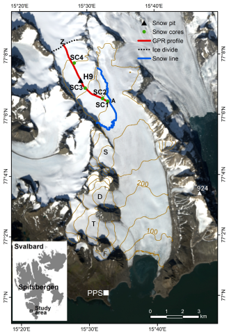
2. Study Area
3. Materials and Methods
3.1. Snow Pits for Snowpack Analysis
3.2. Snow Cover Survey by Ground Penetrating Radar (GPR)
3.3. Combination of GPR Structure with the Snowpack Properties
4. Results
4.1. Overview of the Snow Properties Based on Snow Pit Analysis
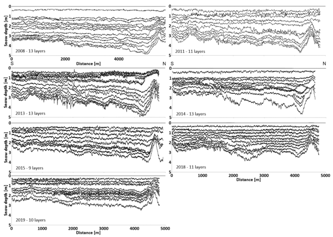
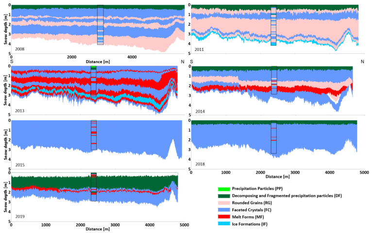
4.2. The Internal Structure of Snow Cover Derived from the GPR Survey
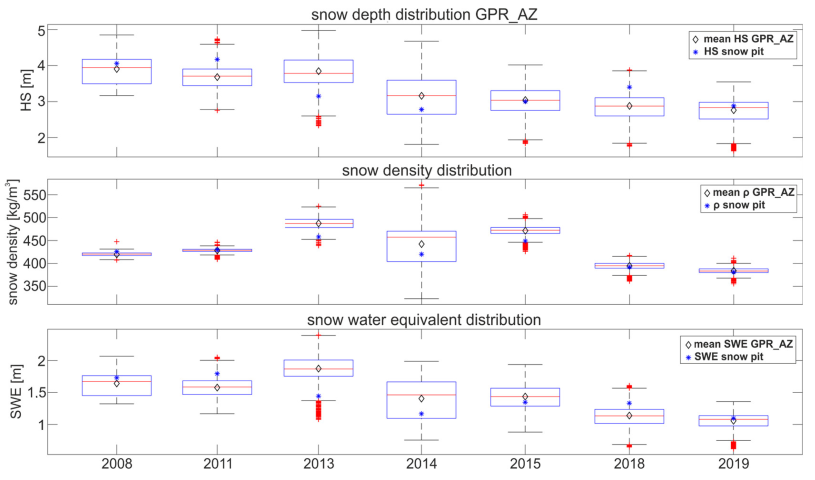
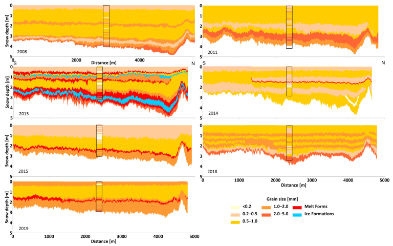
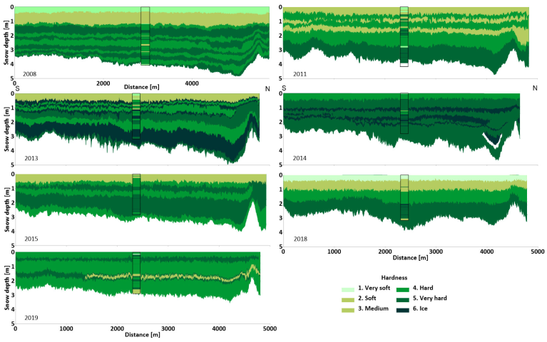
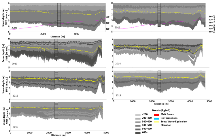
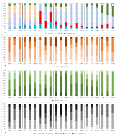
4.3. The Properties of the Snow Layers in the GPR Profiles
5. Discussion
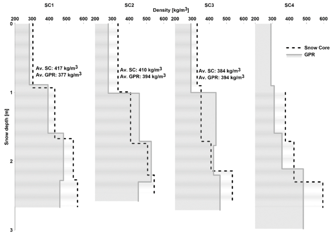
5.1. Limitations of the Transfer of Snow Properties between the Snow Pit and the GPR Profile
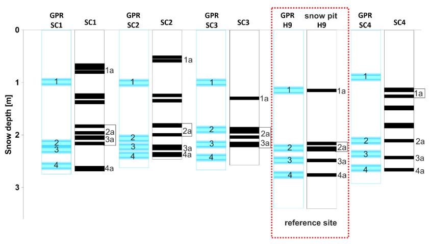
5.2. Validation of Selected Snow Cover Features
5.3. General Regularities in the Structure of the Snow Cover
5.4. HS and AR Characteristics
5.5. Factors Influencing Bulk Density and Its Spatial and Temporal Variability
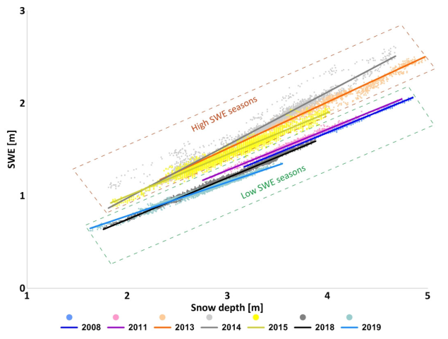
5.6. Temporal and Spatial Variability of SWE
5.7. The HLs in Nival Systems of Glaciers
6. Conclusions
- The snow cover structure is variable in space and from season to season. The extrapolation of snow pit data through radar profiling is a novel solution that can improve the spatial recognition of snow cover characteristics and the accuracy of SWE calculations;
- The location of the H9 snow pit was representative of the center line in the accumulation zone of Hansbreen;
- The snow cover layers were predominantly continuous, with just isolated cases of discontinued ones. Difficulties in identifying layers mainly occurred in the ice divide due to the reduction in the HS and individual layers due to blowing out;
- In 2008–2019 HS showed a downward trend. The mean AR along the center line of the accumulation field was lower than the average for the entire Hansbreen, mainly due to the atypical reduction in the HS in the most elevated areas of the ice divide;
- FC layers predominated in the snowpack structure (51% on average). The standard snowpack structure included DF (or PP) at the top and FC (or RG) at the bottom. The layers were separated by inserts of IF and MF layers (especially in the lower part of the profile). Harder and denser layers occurred in the middle and lower parts and were interspersed with layers of lower density and hardness;
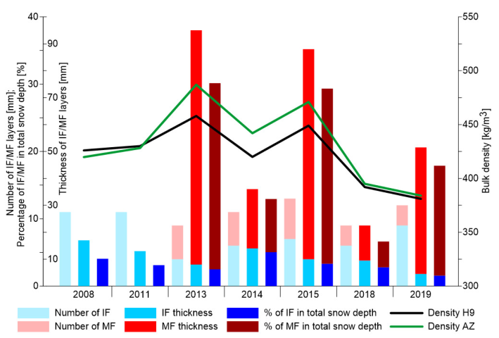
- Numerous HLs were observed in the accumulation zone along the center line (contributing up to 30% of the snow column), but there was no trend in quantity, thickness, or percentage contribution to total snow depth. The substantial HL contribution to the snowpack significantly increased the bulk density.
- IF layers form barriers for air and water vapor circulation within the snowpack and for the percolation of rain or meltwater. HLs with strong crystal bonds create a “frame” in the snowpack, which reduces compaction. As a consequence, IF layers slow down the rate of metamorphosis of the snowpack.
Author Contributions
Funding
Data Availability Statement
Acknowledgments
Conflicts of Interest
References
- Armstrong, R.L.; Brown, R. Introduction. In Snow and Climate. Physical Processes, Surface Energy Exchange and Modelling; Armstrong, R.L., Brun, E., Eds.; Cambridge University Press: Cambridge, UK, 2008; pp. 1–11. [Google Scholar]
- Warren, S.G.; Rigor, I.G.; Untersteiner, N.; Radionov, V.R.; Bryazgin, N.N.; Aleksandrov, Y.I.; Colony, R. Snow depth on arctic sea ice. J. Climate 1999, 12, 1814–1829. [Google Scholar] [CrossRef]
- Cohen, J.L.; Rind, D. The effect of snow cover on the climate. J. Climate 1991, 4, 689–706. [Google Scholar] [CrossRef]
- Jonsell, U.; Hock, R.; Holmgren, B. Spatial and temporal variations in albedo on Storglaciären, Sweden. J. Glaciol. 2003, 49, 59–68. [Google Scholar] [CrossRef] [Green Version]
- Fujita, K. Influence of precipitation seasonality on glacier mass balance and its sensitivity to climate change. Ann. Glaciol. 2008, 48, 88–92. [Google Scholar] [CrossRef] [Green Version]
- Benn, D.I.; Evans, D.J.A. Glaciers and Glaciation, 2nd ed.; Hodder Education: London, UK, 2010; 816p. [Google Scholar]
- Colbeck, S.C. An overview of seasonal snow metamorphism. Rev. Geophys. 1982, 20, 45–61. [Google Scholar] [CrossRef]
- Fierz, C.; Armstrong, R.L.; Durand, Y.; Etchevers, P.; Greene, E.; Mcclung, D.M.; Nishimura, K.; Satyawali, P.K.; Sokratov, S.A. The International Classification for Seasonal Snow on the Ground; IACS Contribution, No. 1; UNESCO-IHP: Paris, France, 2009; p. 90. [Google Scholar]
- Valt, M.; Salvatori, R. Snowpack characteristics of Brøggerhalvøya, Svalbard Islands. Rend. Fis. Acc. Lincei 2016, 27 (Suppl. S1), 129–136. [Google Scholar] [CrossRef]
- Cuffey, K.M.; Paterson, W.S.B. The Physics of Glaciers; Academic Press: London, UK, 2010; 704p. [Google Scholar]
- Callaghan, T.V.; Johansson, M.; Brown, R.D.; Groisman, P.Y.; Labba, N.; Radionov, V.; Barry, R.G.; Bulygina, O.N.; Essery, R.L.; Frolov, D.M.; et al. The Changing Face of Arctic Snow Cover: A Synthesis of Observed and Projected Changes. AMBIO 2011, 40, 17–31. [Google Scholar] [CrossRef] [Green Version]
- Moreno, R.M.; Canadas, E.S. Snow cover evolution in the High Arctic, Nordenskiöld Land (Spitsbergen, Svalbard). Bol. Asoc. Geógr. Esp. 2013, 61, 409–413. [Google Scholar]
- Jansson, P.; Hock, R.; Schneider, T. The concept of glacier storage: A review. J. Hydrol. 2003, 282, 116–129. [Google Scholar] [CrossRef]
- Hodgkins, R.; Cooper, R.; Wadham, J.; Trantner, M. Interannual variability in the spatial distribution of winter accumulation at a high-Arctic glacier (Finsterwalderbreen, Svalbard), and its relationship with topography. Ann. Glaciol. 2005, 24, 243–248. [Google Scholar] [CrossRef] [Green Version]
- Decaux, L.; Grabiec, M.; Ignatiuk, D.; Jania, J. Role of discrete water recharge from supraglacial drainage systems in modeling patterns of subglacial conduits in Svalbard glaciers. Cryosphere 2019, 13, 735–752. [Google Scholar] [CrossRef]
- Barbaro, E.; Koziol, K.; Björkman, M.P.; Vega, C.P.; Zdanowicz, C.; Martma, T.; Gallet, J.-C.; Kępski, D.; Larose, C.; Luks, B.; et al. Measurement report: Spatial variations in ionic chemistry and water-stable isotopes in the snowpack on glaciers across Svalbard during the 2015–2016 snow accumulation season. Atmos. Chem. Phys. 2021, 21, 3163–3180. [Google Scholar] [CrossRef]
- Koziol, K.; Uszczyk, A.; Pawlak, F.; Frankowski, M.; Polkowska, Z. Seasonal and Spatial Differences in Metal and Metalloid Concentrations in the Snow Cover of Hansbreen, Svalbard. Front. Earth Sci. 2021, 8, 538762. [Google Scholar] [CrossRef]
- Spolaor, A.; Moroni, B.; Luks, B.; Nawrot, A.; Roman, M.; Larose, C.; Stachnik, Ł.; Bruschi, F.; Kozioł, K.; Pawlak, F.; et al. Investigation on the Sources andImpact of Trace Elements in the Annual Snowpack and the Firn in the Hansbreen (Southwest Spitsbergen). Front. Earth Sci. 2021, 8, 536036. [Google Scholar] [CrossRef]
- Lewandowski, M.; Kusiak, M.A.; Werner, T.; Nawrot, A.; Barzycka, B.; Laska, M.; Luks, B. Seeking the Sources of Dust: Geochemical and Magnetic Studies on “Cryodust” in Glacial Cores from Southern Spitsbergen (Svalbard, Norway). Atmosphere 2020, 11, 1325. [Google Scholar] [CrossRef]
- Meinander, O.; Dagsson-Waldhauserova, P.; Amosov, P.; Aseyeva, E.; Atkins, C.; Baklanov, A.; Baldo, C.; Barr, S.L.; Barzycka, B.; Benning, L.G.; et al. Newly identified climatically and environmentally significant high-latitude dust sources. Atmos. Chem. Phys. 2022, 22, 11889–11930. [Google Scholar] [CrossRef]
- Stocker, T.F.; Qin, D.; Plattner, G.-K.; Tignor, M.; Allen, S.K.; Boschung, J.; Nauels, A.; Xia, Y.; Bex, V.; Midgley, P.M. Climate Change 2013: The Physical Science Basis; Contribution of Working Group I to the Fifth Assessment Report of the Intergovernmental Panel on Climate Change (IPCC); Cambridge University: Cambridge, UK; New York, NY, USA, 2013; p. 1535. [Google Scholar] [CrossRef] [Green Version]
- Isaksen, K.; Nordli, O.; Forland, E.J.; Łupikasza, E.; Eastwood, S.; Niedźwiedź, T. Recent warming on Spitsbergen—Influence of atmospheric circulation and sea ice cover. J. Geophys. Res. Atmos. 2016, 121, 11913–11931. [Google Scholar] [CrossRef]
- Hanssen-Bauer, I.; Førland, E.J.; Hisdal, H.; Mayer, S.; Sandø, A.B.; Sorteberg, A. (Eds.) Climate in Svalbard 2100–A Knowledge Base for Climate Adaptation; NCCS Report 1/2019; Norwegian Centre of Climate Services (NCCS) for Norwegian Environment Agency (Miljødirektoratet): Oslo, Norway, 2019; 208p. [Google Scholar] [CrossRef]
- Wawrzyniak, T.; Osuch, M. A 40-year High Arctic climatological dataset of the Polish Polar Station Hornsund (SWSpitsbergen, Svalbard). Earth Syst. Sci. Data 2020, 12, 805–815. [Google Scholar] [CrossRef] [Green Version]
- Vikhamar-Schuler, D.; Isaksen, K.; Haugen, J.E.; Tømmervik, H.; Luks, B.; Schuler, T.V.; Bjerke, J.W. Changes in winter warming events in the Nordic Arctic Region. J. Clim. 2016, 29, 6223–6244. [Google Scholar] [CrossRef]
- Łupikasza, E.B.; Ignatiuk, D.; Grabiec, M.; Cielecka-Nowak, K.; Laska, M.; Jania, J.; Luks, B.; Uszczyk, A.; Budzik, T. The role of winter rain in the glacial system on Svalbard. Water 2019, 11, 334. [Google Scholar] [CrossRef] [Green Version]
- McBean, G. Arctic Climate: Past and Present (Chapter 2). In Arctic Climate Impact Assessment; Symon, C., Arris, L., Heal, B., Eds.; ACIA Scientific Report; Cambridge University Press: Cambridge, UK, 2005; pp. 21–60. [Google Scholar]
- Vickers, H.; Karlsen, S.R.; Malnes, E. A 20-Year MODIS-Based Snow Cover Dataset for Svalbard and Its Link to Phenological Timing and Sea Ice Variability. Remote Sens. 2020, 12, 1123. [Google Scholar] [CrossRef] [Green Version]
- Screen, J.; Simmonds, I. The central role of diminishing sea ice in recent Arctic temperature amplification. Nature 2010, 464, 1334–1337. [Google Scholar] [CrossRef] [Green Version]
- Serreze, M.C.; Barry, R.G. Processes and impacts of Arctic amplification: A research synthesis. Glob. Planet. Chang. 2011, 77, 85–96. [Google Scholar] [CrossRef]
- Maturilli, M.; Herber, A.; Konig-Langlo, G. Climatology and time series of surface meteorology in Ny-Ålesund, Svalbard. Earth Syst. Sci. Data 2013, 5, 155–163. [Google Scholar] [CrossRef] [Green Version]
- Hansen, B.B.; Isaksen, K.; Benestad, R.E.; Kohler, J.; Pedersen, Å.Ø.; Loe, L.E.; Coulson, S.J.; Larsen, J.O.; Varpe, Ø. Warmer and wetter winters: Characteristics and implications of an extreme weather event in the High Arctic. Environ. Res. Lett. 2014, 9, 114021. [Google Scholar] [CrossRef]
- Nordli, Ø.; Przybylak, R.; Ogilvie, A.E.J.; Isaksen, K. Long-term temperature trends and variability on Spitsbergen: The extended Svalbard airport temperature series, 1898–2012. Polar Res. 2014, 33, 1898–2012. [Google Scholar] [CrossRef] [Green Version]
- AMAP Assessment 2021: Mercury in the Arctic; Arctic Monitoring and Assessment Programme (AMAP): Tromsø, Norway, 2021; 324p.
- Grabiec, M. Stan i Współczesne Zmiany Systemów Lodowcowych Południowego Spitsbergenu w Świetle Badań Metodami Radarowymi [The State and Contemporary Changes of Glacial Systems in Southern Spitsbergen in the Light of Radar Methods]; Wydawnictwo Uniwersytetu Śląskiego: Katowice, Poland, 2017; 328p. [Google Scholar]
- Graham, R.M.; Cohen, L.; Petty, A.A.; Boisvert, L.N.; Rinke, A.; Hudson, S.R.; Nicolaus, M.; Granskog, M.A. Increasing frequency and duration of Arctic winter warming events. Geophys. Res. Lett. 2017, 44, 6974–6983. [Google Scholar] [CrossRef] [Green Version]
- Peeters, B.; Pedersen, A.O.; Loe, E.L.; Isaksen, K.; Veiberg, V.; Stein, A.; Kohler, J.; Gallet, J.-C.; Aanes, R. Spatiotemporal patterns of rain-on-snow and basal ice in high Arctic Svalbard. Detection of a climate-cryosphere regime shift. Environ. Res. Lett. 2019, 14, 015002. [Google Scholar] [CrossRef]
- Nowak, A.; Hodson, A. Hydrological response of a High-Arctic catchment to changing climate over the past 35 years: A case study of Bayelva watershed, Svalbard. Polar Res. 2013, 32, 19691. [Google Scholar] [CrossRef]
- Bintanja, R.; Selten, F.M. Future increases in Arctic precipitation linked to local evaporation and sea-ice retreat. Nature 2014, 509, 479–482. [Google Scholar] [CrossRef]
- Rennert, K.J.; Roe, G.; Putkonen, J.; Bitz, C.M. Soil thermal and ecological impacts of rain on snow events in the circumpolar arctic. J. Clim. 2009, 22, 2302–2315. [Google Scholar] [CrossRef] [Green Version]
- Bintanja, R.; Andry, O. Towards a rain-dominated Arctic. Nat. Clim. Chang. 2017, 7, 263–267. [Google Scholar] [CrossRef]
- Sobota, I.; Weckwerth, P.; Grajewski, T. Rain-On-Snow (ROS) events and their relations to snowpack and ice layer changes on small glaciers in Svalbard, the high Arctic. J. Hydrol. 2020, 590, 125279. [Google Scholar] [CrossRef]
- Laska, M.; Luks, B.; Budzik, T. Influence of snowpack internal structure on snow metamorphism and melting intensity on Hansbreen, Svalbard. Pol Polar Res. 2016, 37, 193–218. [Google Scholar] [CrossRef] [Green Version]
- Blatter, H.; Hutter, K. Polythermal conditions in Arctic glaciers. J. Glaciol. 1991, 37, 261–269. [Google Scholar] [CrossRef] [Green Version]
- Ahlmann, H.W. Scientific results of the Swedish−Norwegian Arctic Expedition in the summer of 1931. Part VIII. Geogr. Ann. 1933, 15, 161–216. [Google Scholar] [CrossRef]
- Ahlmann, H.W. The Fourteenth of July Glacier scientific results of the Norwegian–Swedish Spitsbergen Expedition in 1934. Part V. Geogr Ann. 1935, 17, 167–211. [Google Scholar] [CrossRef]
- Migała, K.; Pereyma, J.; Sobik, M. Snow accumulation in South Spitsbergen. In Wyprawy Polarne Uniwersytetu Śląskiego 1980–1984; Jania, J., Pulina, M., Eds.; University of Silesia: Katowice, Poland, 1988; Volume 2, pp. 48–63. [Google Scholar]
- Tveit, J.; Killingtveit, Ĺ. Snow surveys for studies of water budget on Svalbard. In Proceedings of the 10th International Northern Research Basins Symposium and Workshop, Spitsbergen, Norway, 28 August–3 September 1994; pp. 489–509. [Google Scholar]
- Grześ, M.; Sobota, I. Winter snow accumulation and winter outflow from the Waldemar Glacier (NW Spitsbergen) between 1996 and 1998. Pol. Polar Res. 2000, 21, 19–32. [Google Scholar]
- Sand, K.; Winther, J.G.; Marechal, D.; Bruland, O.; Melvold, K. Regional variations of snow accumulation on Spitsbergen, Svalbard in 1997–99. Hydrol. Res. 2003, 34, 17–32. [Google Scholar] [CrossRef]
- Małecki, J. Snow accumulation on a small high-arctic glacier Svenbreen—Variability and topographic controls. Geogr. Ann. Ser. A Phys. Geogr. 2016, 97, 809–817. [Google Scholar] [CrossRef]
- Möller, M.; Möller, R.; Beaudon, É.; Mattila, O.-P.; Finkelnburg, R.; Braun, M.; Grabiec, M.; Jonsell, U.; Luks, B.; Puczko, D.; et al. Snowpack characteristics of Vestfonna and De Geerfonna (Nordaustlandet, Svalbard)—A spatiotemporal analysis based on multiyear snow-pit data. Geogr. Ann. Ser. A Phys. Geogr. 2011, 93, 273–285. [Google Scholar] [CrossRef]
- Sobota, I. Snow accumulation, melt, mass loss, and the near-surface ice temperature structure of Irenebreen, Svalbard. Polar Sci. 2011, 5, 327–336. [Google Scholar] [CrossRef] [Green Version]
- Sobota, I. Współczesne Zmiany Kriosfery Północnozachodniego Spitsbergenu na Przykładzie regionu Kaffiøyry [Contemporary Changes of the Cryosphere of North-Western Spitsbergen Based on the Example of the Kaffioyra Region]; Wydawnictwo Naukowe UMK: Toruń, Poland, 2013; 449p. (In Polish) [Google Scholar]
- Sobota, I. Selected problems of snow accumulation on glaciers during long-term studies in north-western Spitsbergen, Svalbard. Geogr. Ann. Ser. A Phys. Geogr. 2017, 92, 177–192. [Google Scholar] [CrossRef]
- Sauter, T.; Möller, M.; Finkelnburg, R.; Grabiec, M.; Scherer, D.; Schneider, C. Snowdrift modelling for the Vestfonna ice cap, north—Eastern Svalbard. Cryosphere 2013, 7, 1287–1301. [Google Scholar] [CrossRef] [Green Version]
- Kosiba, A. Badania glacjologiczne na Spitsbergenie w lecie 1957 roku [Glaciological investigations of the Polish IGY Spitsbergen Expedition in 1957]. Prz. Geofiz. 1958, 3, 95–122, [In Polish]. [Google Scholar]
- Kosiba, A. Some of Results of Glaciological Investigations in SW-Spitsbergen. Carried out during the Polish I. G. Y. Spitsbergen Expeditions in 1957, 1958 and 1959; Zeszyty Naukowe. Ser. B. Nauki Przyrodnicze 4. Nauka O Ziemi, 3–14; Uniwersytet Wrocławski Im. Bolesława Bieruta/Państwowe Wydawnictwo Naukowe: Warsaw, Poland, 1960. [Google Scholar]
- Baranowski, S. Report on the Field Work of the Polish Scientific Expedition in 1973; Wydawnictwo Uniwersytetu Wrocławskiego: Wrocław, Poland, 1974; 29p. [Google Scholar]
- Baranowski, S. The subpolar glaciers of Spitsbergen seen against the climate of this region. Acta Univ. Wratislav. 1977, 410, 1–94. [Google Scholar]
- Jania, J. Field Investigations during Glaciological Expeditions to Spitsbergen in the Period 1992–1994; Interim Report; University of Silesia: Katowice, Poland, 1994; 40p. [Google Scholar]
- Grabiec, M.; Budzik, T.; Głowacki, P. Modelling and Hindcasting of the Mass Balance of Werenskioldbreen (Southern Svalbard). Arct. Antarct. Alp. Res. 2012, 44, 164–179. [Google Scholar] [CrossRef] [Green Version]
- Pulina, M. Stratification and physic-chemical properties of snow in Spitsbergen in the hydro-glaciological year 1989/1990. In Wyprawy Geograficzne na Spitsbergen; UMCS: Lublin, Poland, 1991; pp. 191–213. [Google Scholar]
- Glazovsky, A.F.; Kolondra, L.; Moskalevsky, M.Y.; Jania, J. Research into Hansbreen, a tidewater glacier in Spitsbergen. Polar Geogr. Geol. 1992, 16, 243–252. [Google Scholar] [CrossRef]
- Leszkiewicz, J.; Pulina, M. Snowfall phases in analysis of snow cover in Hornsund, Spitsbergen. Pol. Polar Res. 1999, 20, 3–24. [Google Scholar]
- Głowacki, P.; Pulina, M. The physico-chemical properties of the snow cover of Spitsbergen (Svalbard) based on investigations during the winter season 1990/1991. Pol. Polar Res. 2000, 21, 65–88. [Google Scholar]
- Głowacki, P. Rola Procesów Fizyczno-Chemicznych w Kształtowaniu Struktury Wewnętrzneji Obiegu Masy Lodowców Spitsbergenu [Role of Physical and Chemical Processes in the Internal Structure Formation and Mass Circulation of Spitsbergen glaciers]; Publications of the Institute of Geophysics Polish Academy of Sciences: Warszawa, Poland, 2007; pp. 1–146. (In Polish) [Google Scholar]
- Nawrot, A.P.; Migała, K.; Luks, B.; Pakszys, P.; Głowacki, P. Chemistry of snow cover and acidic snowfall during a season with a high level of air pollution on the Hans Glacier, Spitsbergen. Polar Sci. 2016, 10, 249–261. [Google Scholar] [CrossRef]
- Uszczyk, A.; Grabiec, M.; Laska, M.; Kuhn, M.; Ignatiuk, D. Importance of snow as component of surface mass balance of Arctic glacier (Hansbreen, southern Spitsbergen). Pol. Polar Res. 2019, 40, 311–338. [Google Scholar] [CrossRef]
- Laska, M.; Luks, B.; Kępski, D.; Gądek, B.; Głowacki, P.; Puczko, D.; Migała, K.; Nawrot, A.; Pętlicki, M. Hansbreen Snowpit Dataset—Over 30-year of detailed snow research on an Arctic glacier. Sci. Data 2022, 9, 656. [Google Scholar] [CrossRef] [PubMed]
- Grabiec, M.; Puczko, D.; Budzik, T.; Gajek, G. Snow distribution patterns on Svalbard glaciers derived from radio-echo soundings. Pol. Polar Res. 2011, 32, 393–421. [Google Scholar] [CrossRef]
- Melvold, K. Snow measurements using GPR: Example from Amundsenisen, Svalbard. In Applied Geophysics in Periglacial Environments; Hauck, C., Kneisel, C., Eds.; Cambridge University Press: Cambridge, UK, 2008; pp. 207–216. [Google Scholar]
- Laska, M.; Grabiec, M.; Ignatiuk, D.; Budzik, T. Snow deposition patterns on southern Spitsbergen glaciers, Svalbard, in relation to recent meteorological conditions and local topography. Geogr. Ann. Phys. Geogr. 2017, 99, 262–287. [Google Scholar] [CrossRef]
- Kohler, J.; Moore, J.; Kennett, M.; Engeset, R.; Elvehøy, H. Using ground-penetrating radar to image previous years summer surfaces for mass-balance measurements. Ann. Glaciol. 1997, 24, 355–360. [Google Scholar] [CrossRef] [Green Version]
- Winther, J.-G.; Bruland, O.; Sand, K.; Killingtveit, Å.; Marechal, D. Snow accumulation distribution on Spitsbergen, Svalbard, in 1997. Polar Res. 1998, 17, 155–164. [Google Scholar] [CrossRef]
- Bruland, O.; Sand, K.; Killingtveit, Å. Snow distribution at a High Arctic site at Svalbard. Nord. Hydrol. 2001, 32, 1–12. [Google Scholar] [CrossRef]
- Pinglot, J.F.; Hagen, J.; Melvold, K.; Eiken, T.; Vincent, C. A mean net accumulation pattern derived from radioactive layers and radar soundings on Austfonna, Nordaustlandet, Svalbard. J. Glaciol. 2001, 47, 555–566. [Google Scholar] [CrossRef] [Green Version]
- Taurisano, A.; Schuler, T.V.; Hagen, J.-O.; Eiken, T.; Loe, E.; Melvold, K.; Kohler, J. The distribution of snow accumulation across the Austfonna ice cap, Svalbard: Direct measurements and modelling. Polar Res. 2007, 26, 7–13. [Google Scholar] [CrossRef]
- Dunse, T.; Schuler, T.; Hagen, J.; Eiken, T.; Brandt, O.; Høgda, K. Recent fluctuations in the extent of the firn area of Austfonna, Svalbard, inferred from GPR. Ann. Glaciol. 2009, 50, 155–162. [Google Scholar] [CrossRef] [Green Version]
- Van Pelt, W.J.J.; Pettersson, R.; Pohjola, V.; Marchenko, S.; Claremar, B.; Oerlemans, J. Inverse estimation of snow accumulation along a snow radar transect on Nordenskiöldbreen, Svalbard. J. Geophys. Res. Earth Surf. 2014, 119, 816–835. [Google Scholar] [CrossRef]
- Singh, G.; Lavrentiev, I.; Glazovsky, A.; Patil, A.; Mohanty, S.; Khromova, T.; Nosenko, G.; Sosnovskiy, A.; Arigony-Neto, J. Retrieval of Spatial and Temporal Variability in Snowpack Depth over Glaciers in Svalbard Using GPR and Spaceborne POLSAR Measurements. Water 2020, 12, 21. [Google Scholar] [CrossRef] [Green Version]
- Mätzler, C. Microwave permittivity of dry snow. IEEE Trans. Geosci. Remote Sens. 1996, 34, 573–581. [Google Scholar] [CrossRef]
- Harper, J.; Bradford, J. Snow stratigraphy over a uniform depositional surface:spatial variability and measurement tools. Cold Reg. Sci. Technol. 2003, 37, 289–298. [Google Scholar] [CrossRef]
- Dunse, T.; Eisen, O.; Helm, V.; Rack, W.; Steinhage, D.; Parry, V. Characteristics and small-scale variability of GPR signals and their relation to snow accumulation in Greenland’s percolation zone. J. Glaciol. 2008, 54, 333–342. [Google Scholar] [CrossRef] [Green Version]
- Jania, J.; Mochnacki, D.; Gądek, B. The thermal structure of Hansbreen, a tidewater glacier in southern Spitsbergen, Svalbard. Polar Res. 1996, 15, 53–66. [Google Scholar] [CrossRef]
- Pälli, A.; Moore, J.C.; Jania, J.; Kolondra, L.; Głowacki, P. The drainage pattern of Hansbreen and Werenskioldbreen, two polythermal glaciers in Svalbard. Polar Res. 2003, 22, 355–371. [Google Scholar] [CrossRef] [Green Version]
- Ignatiuk, D.; Piechota, A.; Ciepły, M.; Luks, B. Changes of altitudinal zones of Werenskioldbreen and Hansbreen in period 1990–2008, Svalbard. AIP Conf. Proc. 2014, 1618, 275–280. [Google Scholar] [CrossRef]
- Błaszczyk, M.; Ignatiuk, D.; Uszczyk, A.; Cielecka-Nowak, K.; Grabiec, M.; Jania, J.A.; Moskalik, M.; Walczowski, W. Freshwater input to the Arctic fjord Hornsund (Svalbard). Polar Res. 2019, 38, 3506. [Google Scholar] [CrossRef]
- Grabiec, M.; Jania, J.; Puczko, D.; Kolondra, L.; Budzik, T. Surface and bed morphology of Hansbreen, a tidewater glacier in Spitsbergen. Pol. Polar Res. 2012, 33, 111–138. [Google Scholar] [CrossRef]
- Laska, M.; Barzycka, B.; Luks, B. Melting characteristics of snow cover on tidewater glaciers in Hornsund fjord, Svalbard. Water 2017, 9, 804. [Google Scholar] [CrossRef]
- Schuler, T.V.; Kohler, J.; Elagina, N.; Hagen, J.O.M.; Hodson, A.J.; Jania, J.A.; Kaab, A.M.; Luks, B.; Małecki, J.; Moholdt, G.; et al. Reconciling Svalbard glacier mass balance. Front. Earth Sci. 2020, 8, 156. [Google Scholar] [CrossRef]
- Błaszczyk, M.; Ignatiuk, D.; Grabiec, M.; Kolondra, L.; Laska, M.; Decaux, L.; Jania, J.; Berthier, E.; Luks, B.; Barzycka, B.; et al. Quality assessment and glaciological applications of digital elevation models derived from space-borne and aerial images over two tidewater glaciers of southern Spitsbergen. Remote Sens. 2019, 11, 1121. [Google Scholar] [CrossRef]
- Niedźwiedź, T. The atmospheric circulation. In Climate and Climate Change at Hornsund, Svalbard; Marsz, A.A., Styszyńska, A., Eds.; Gdynia Maritime University: Gdynia, Poland, 2013; pp. 57–74. [Google Scholar]
- Wawrzyniak, T.; Osuch, M. A consistent High Arctic climatological dataset (1979–2018) of the Polish Polar Station Hornsund (SW Spitsbergen, Svalbard). PANGAEA 2019. [Google Scholar]
- Łupikasza, E. Atmospheric precipitation. In Climate and Climate Change at Hornsund, Svalbard; Marsz, A.A., Styszyńska, A., Eds.; Gdynia Maritime University: Gdynia, Poland, 2013; pp. 199–211. [Google Scholar]
- Grabiec, M.; Leszkiewicz, J.; Głowacki, P.; Jania, J. Distribution of snow accumulation on some glaciers of Spitsbergen. Pol. Polar Res. 2006, 27, 309–326. [Google Scholar]
- Styszyńska, A. The winds. In Climate and Climate Change at Hornsund, Svalbard; Marsz, A.A., Styszyńska, A., Eds.; Gdynia Maritime University: Gdynia, Poland, 2013; pp. 81–99. [Google Scholar]
- Colbeck, S.C.; Akitaya, E.; Armstrong, R.L.; Gubler, H.; Lafeuille, J.; Lied, K.; McClung, D.M.; Morris, E.M. The International Classification for Seasonal Snow on the Ground; International Commission on Snow and Ice (IAHS), World Data Center A for Glaciology, University of Colorado: Boulder, CO, USA, 1990. [Google Scholar]
- Neal, A. Ground-Penetrating Radar and its use in sedimentology: Principles, problems and progress. Earth-Sci. Rev. 2004, 66, 261–330. [Google Scholar] [CrossRef]
- Hubbard, B.; Glasser, N. Field Techniques in Glaciology and Glacial Geomorphology; John Wiley & Sons, Ltd.: Chichester, UK, 2005; 400p. [Google Scholar]
- Berthling, I.; Melvold, K. Ground-penetrating radar. In Applied Geophysics in Periglacial Environments; Hauck, C., Kneisel, C., Eds.; Cambridge University Press: Cambridge, UK, 2008; pp. 81–98. [Google Scholar]
- Barzycka, B.; Grabiec, M.; Błaszczyk, M.; Ignatiuk, D.; Laska, M.; Hagen, J.O.; Jania, J. Changes of glacier facies on Hornsund glaciers (Svalbard) during the decade 2007–2017. Remote Sens. Environ. 2020, 251, 112060. [Google Scholar] [CrossRef]
- Hamed, K.H.; Rao, A.R. A Modified Mann-Kendall Trend Test for Autocorrelated Data. J. Hydrol. 1998, 204, 182–196. [Google Scholar] [CrossRef]
- Heilig, A.; Schneebeli, M.; Eisen, O. Upward-looking ground-penetrating radar for monitoring snowpack stratigraphy. Cold Reg. Sci. Technol. 2009, 59, 152–162. [Google Scholar] [CrossRef]
- Yamamoto, T.; Matsuoka, K.; Naruse, R. Observation of internal structures of snow covers with a ground-penetrating radar. Ann. Glaciol. 2004, 38, 21–24. [Google Scholar] [CrossRef]
- Marshall, H.-P.; Schneebeli, M.; Koh, G. Snow Stratigraphy Measurements with High-Frequency FMCW Radar: Comparison with Snow Micro-Penetrometer. Cold Reg. Sci. Technol. 2007, 47, 108–117. [Google Scholar] [CrossRef]
- Wadham, J.; Nuttall, A. Multiphase formation of superimposed ice during a mass-balance year at a maritime high-Arctic glacier. J. Glaciol. 2002, 48, 545–551. [Google Scholar] [CrossRef] [Green Version]
- Marchand, W.D.; Killingtveit, A. Statistical properties of spatial snowcover inmountainous catchments in Norway. Nord. Hydrol. 2004, 35, 101–117. [Google Scholar] [CrossRef]
- Lundberg, A.; Richardson–Naslund, C.; Andersson, C. Snow density variations:consequences for ground-penetrating radar. Hydrol. Process. 2006, 20, 1483–1495. [Google Scholar] [CrossRef]
- Jonas, T.; Marty, C.; Magnusson, J. Estimating the snow water equivalent from snow depth measurements in the Swiss Alps. J. Hydrol. 2009, 378, 161–167. [Google Scholar] [CrossRef]
- Jordan, R.E.; Albert, M.R.; Brun, E. Physical processes within the snow cover and their parameterization. In Snow and Climate Physical Processes, Surface Energy Exchange and Modeling; Armstrong, R.L., Brun, E., Eds.; Cambridge University Press: Cambridge, UK, 2008; pp. 12–69. [Google Scholar]
- Szafraniec, J. Influence of positive degree-days and sunshine duration on the Surface ablation of Hansbreen, Spitsbergen glacier. Pol. Polar Res. 2002, 23, 227–240. [Google Scholar]


| GPR Date | Snow Pit—Closest Distance to the GPR Profile [m] | Sampling Frequency [MHz] | Samples | Time Interval [s] | Time Window [ns] | Snow Pit Date |
|---|---|---|---|---|---|---|
| 26 April 2008 | - | 5116.6 | 512 | 0.5 | 100.07 | 23, 24 April 2008 |
| 14 and 17 April 2011 | 15.1 | 12,791.6 | 1024 | 0.2 | 80.05 | 16 April 2011 |
| 16 and 17 April 2013 | 38.8 | 12,791.6 | 1024 | 0.2 | 80.05 | 11 May 2013 |
| 3 and 12 April 2014 | 20.9 | 12,791.6 | 1024 | 0.2 | 80.05 | 6 May 2014 |
| 2 April 2015 | 4 | 5149.2 | 512 | 0.2 | 99.43 | 29 April 2015 |
| 18 and 19 April 2018 | 13.4 * | 16,410.2 | 1324 | 0.2 | 80.68 | 24 April 2018 |
| 6 April 2019 | 1.75 | 12,763.5 | 1030 | 0.2 | 80.70 | 6 May 2019 |
| 2008 | 2011 | 2013 | 2014 | 2015 | 2018 | 2019 | Average | |
|---|---|---|---|---|---|---|---|---|
| Snow depth (HS) in H9 [m] | 4.06 | 4.17 | 3.15 | 2.78 | 3 | 3.4 | 2.88 | 3.35 |
| Average snow depth (HS) along GPR_AZ (min-max) [m] | 3.91 (3.17–4.85) | 3.68 (2.75–4.74) | 3.84 (2.33–4.97) | 3.16 (1.81–4.68) | 3.04 (1.83–4.02) | 2.88 (1.76–3.88) | 2.76 (1.63–3.55) | 3.32 |
| Average accumulation rate (AR) along GPR_AZ [m 100 m−3] | 0.72 | 0.54 | 0.33 | 0.98 | 0.65 | 0.26 | 0.43 | 0.56 |
| Number of layers in H9 (snow pit) | 40 | 39 | 26 | 25 | 25 | 25 | 28 | 29.71 |
| Number of layers in GPR_AZ (GPR profile) | 13 | 11 | 13 | 13 | 9 | 11 | 10 | 11.43 |
| % of layers identified in GPR_AZ | 33 | 28 | 50 | 52 | 36 | 44 | 36 | 39.86 |
Disclaimer/Publisher’s Note: The statements, opinions and data contained in all publications are solely those of the individual author(s) and contributor(s) and not of MDPI and/or the editor(s). MDPI and/or the editor(s) disclaim responsibility for any injury to people or property resulting from any ideas, methods, instructions or products referred to in the content. |
© 2022 by the authors. Licensee MDPI, Basel, Switzerland. This article is an open access article distributed under the terms and conditions of the Creative Commons Attribution (CC BY) license (https://creativecommons.org/licenses/by/4.0/).
Share and Cite
Kachniarz, K.; Grabiec, M.; Ignatiuk, D.; Laska, M.; Luks, B. Changes in the Structure of the Snow Cover of Hansbreen (S Spitsbergen) Derived from Repeated High-Frequency Radio-Echo Sounding. Remote Sens. 2023, 15, 189. https://doi.org/10.3390/rs15010189
Kachniarz K, Grabiec M, Ignatiuk D, Laska M, Luks B. Changes in the Structure of the Snow Cover of Hansbreen (S Spitsbergen) Derived from Repeated High-Frequency Radio-Echo Sounding. Remote Sensing. 2023; 15(1):189. https://doi.org/10.3390/rs15010189
Chicago/Turabian StyleKachniarz, Kamil, Mariusz Grabiec, Dariusz Ignatiuk, Michał Laska, and Bartłomiej Luks. 2023. "Changes in the Structure of the Snow Cover of Hansbreen (S Spitsbergen) Derived from Repeated High-Frequency Radio-Echo Sounding" Remote Sensing 15, no. 1: 189. https://doi.org/10.3390/rs15010189