A Machine-Learning Approach to Intertidal Mudflat Mapping Combining Multispectral Reflectance and Geomorphology from UAV-Based Monitoring

Abstract

Remote sensing is a relevant method to map inaccessible areas, such as intertidal mudflats. However, image classification is challenging due to spectral similarity between microphytobenthos and oyster reefs. Because these elements are strongly related to local geomorphic features, including biogenic structures, a new mapping method has been developed to overcome the current obstacles. This method is based on unmanned aerial vehicles (UAV), RGB, and multispectral (four bands: green, red, red-edge, and near-infrared) surveys that combine high spatial resolution (e.g., 5 cm pixel), geomorphic mapping, and machine learning random forest (RF) classification. A mudflat on the Atlantic coast of France (Marennes-Oléron bay) was surveyed based on this method and by using the structure from motion (SfM) photogrammetric approach to produce orthophotographs and digital surface models (DSM). Eight classes of mudflat surface based on indexes, such as NDVI and spectral bands normalised to NIR, were identified either on the whole image (i.e., standard RF classification) or after segmentation into five geomorphic units mapped from DSM (i.e., geomorphic-based RF classification). The classification accuracy was higher with the geomorphic-based RF classification (93.12%) than with the standard RF classification (73.45%), showing the added value of combining topographic and radiometric data to map soft-bottom intertidal areas and the user-friendly potential of this method in applications to other ecosystems, such as wetlands or peatlands.

1. Introduction

Intertidal mudflats occupy more than 120,000 km² in the world [1] and are characterised by soft sediments subaerially exposed at each low tide. Mudflats provide multiple ecosystem services [2] that are underestimated and often overlooked [3]. Among the most efficient primary producers within coastal ecosystems [4,5,6], mudflat habitats also have a significant potential to cope with the current biodiversity-climate crisis and thus contribute to a number of United Nations and European Union priorities regarding carbon neutrality, climate resilience, biodiversity support, and human well-being [7]. As such, mapping mudflat biodiversity, biomass, and carbon uptake, notably through its main primary producer, the microphytobenthos (MPB), is a milestone that needs to be urgently reached. The unicellular microalgae and prokaryote communities inhabiting muddy surface sediment and forming biofilms exposed at low tide are known for their photosynthetic capacity, and, thus, their carbon uptake efficiency [5,8,9,10]. The current challenges are due to the highly heterogeneous and patchy distribution of intertidal primary producers and the difficulty of accessing mudflats. The harshness and remoteness of these environments often impede any extensive and representative assessment of the biodiversity, biomass, and carbon uptake. They include bare mud potentially colonized by different functional types of MPB [11,12], but also oyster [13] or polychaete Sabellaria alvaeolata reefs [14]. Intertidal surfaces are globally flat, but tidal channels, ridges, and runnels increase heterogeneity and patchiness. Moreover, artificial infrastructures, such as dikes or other hard sea defenses, pontoons, recreational areas or professional fisheries, and shellfish farms, can increase the complexity of these environments.

Over the last decade, remote sensing has demonstrated its potential to fill the gaps by addressing the challenges posed by this difficult environment, with multiple studies conducted using satellite imagery [1,5,10,13,15] involving the mapping of large areas at various timescales. However, the low spatial resolution of these images (at best 10 × 10 m per pixel for non-commercial ESA Sentinel 2 satellite) generates spectral mixing resulting from spatial heterogeneity and patchiness [16] that can create inaccuracies in detecting the actual diversity and biomass of vegetation and habitats. It also hinders accurate evaluation of their carbon uptake [5]. Recent developments in unmanned aerial vehicle (UAV) technology are reducing the constraints of spectral mixing by capturing very high spatial resolution images within a centimetre accuracy range, as well as enabling the production of detailed geomorphic maps [17,18,19,20,21]. Moreover, UAV can collect images with a higher survey frequency within a semi-diurnal tidal cycle, or under cloudy conditions, when no image can be acquired by satellite, or when satellite overpass does not coincide with the lowest tides. Based on machine learning or geographic object-based image Analysis (GEOBIA), previous studies have used UAV-derived RGB (red, green, and blue) and multispectral images, processed through the structure from motion—multi-view stereo (SfM-MVS) photogrammetry technique to map intertidal vegetation, such as seagrasses [22,23], oyster reefs [24], or polychaete reefs [14,25,26,27]. A main constraint of applying these methods to intertidal mudflats is the confusion between MPB and oysters or rocks covered by epibionts that share a similar spectral signature, making their distinction difficult with multispectral indices, but also with more elaborate machine-learning methods, as demonstrated by aerial and close-range hyperspectral and multispectral satellite surveys [28,29].

This constraint is addressed by the present study: distinguishing intertidal vegetation with a focus on the main primary producer, the MPB, from other intertidal elements. To reach our goal, we propose a new method, combining for the first time a morphometric analysis and a machine-learning algorithm (i.e., random forest, RF), applied to high spatial resolution RGB and multispectral images. This method consists of the segmentation of the intertidal zone into geomorphic units, followed by a RF classification over each unit. This approach is supported by the innovative use of elevation end-products of SfM-MVS photogrammetry, i.e., digital surface models (DSM), to provide geomorphic unit maps of mudflats. A standard RF classification solely based on multispectral reflectance was compared with a classification integrating geomorphic units to highlight the higher accuracy achieved by considering the mudflat geomorphology in the processing workflow.

2. Materials and Methods

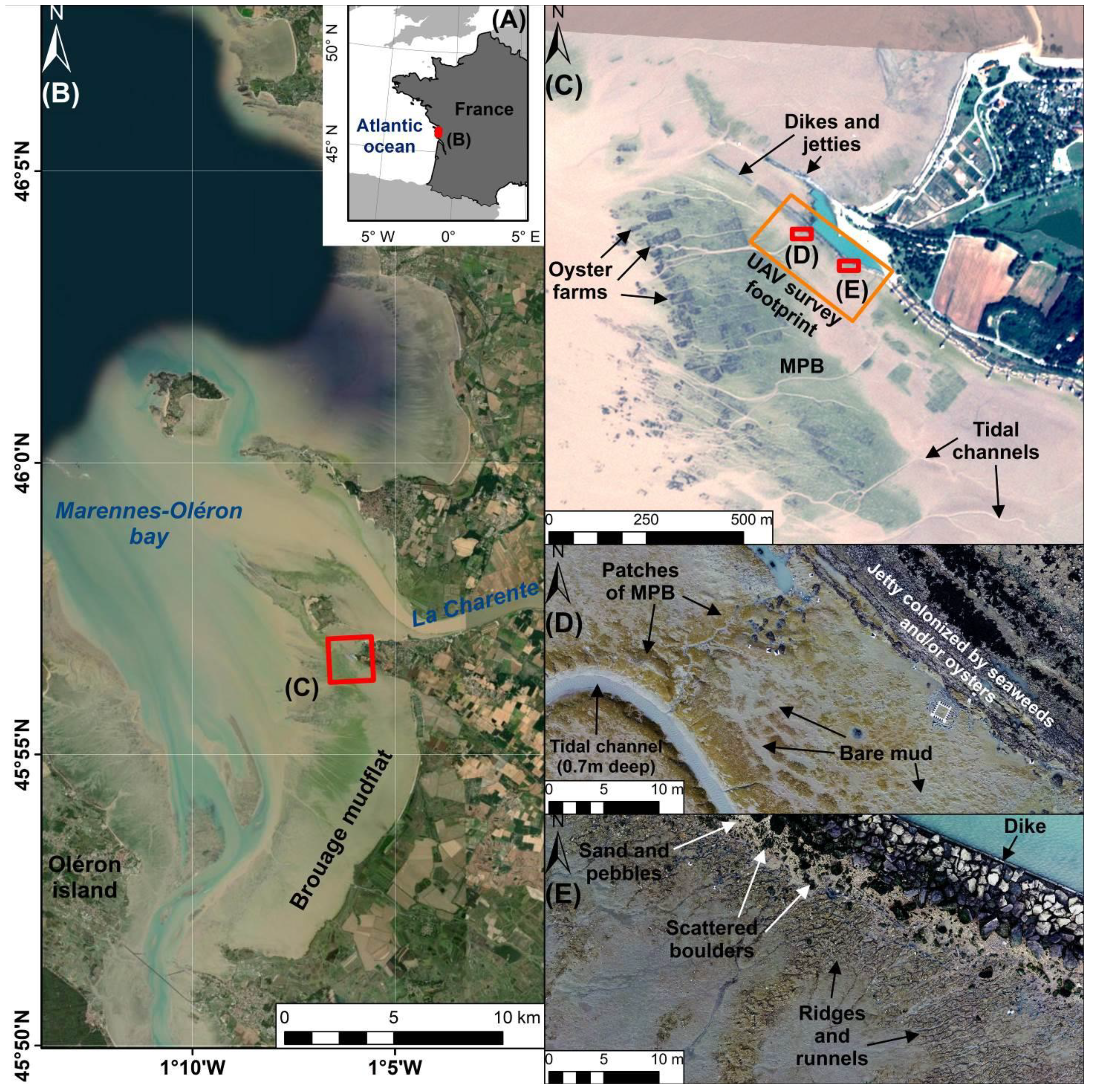
2.1. Study Site

The study site is located in the Pertuis Charentais Sea, a shallow semi-enclosed sea located on the French Atlantic coast (Figure 1A,B), where tides are semi-diurnal with a macrotidal range of 6 m during spring tides [5]. This area is known for its oyster farming and intertidal mudflat environment [2], including the Brouage mudflat (Figure 1A). Oriented north-south, this mudflat extends 10 km southward from the Charente estuary, and is partially protected from western offshore waves by Oléron Island. The consequence is the settling of the mud in suspension from the Charente River, creating mudflats [30,31] hosting large surfaces covered by MPB and oyster farms (Figure 1C). Within the Brouage mudflat, the current study focused on an engineered mudflat with a recreational area comprising an artificial basin enclosed by rocky dikes, a concrete jetty, and oyster farms 200 m from the shore (Figure 1C). Classical mudflat bedforms were observed, such as tidal channels and low-lying ridges and runnels. Reefs, dikes, and jetties were covered by abundant seaweeds, such as brown (Fucus spp.) and green algae (Ulva spp.), but also by wild oysters. Sand, pebbles, and scattered boulders can be observed near the dikes and jetties. MPB showed a patchy distribution with scattered colonies of varied size, surrounded by bare mud, and with the highest densities occurring around tidal channels and oyster reefs (Figure 1D,E).

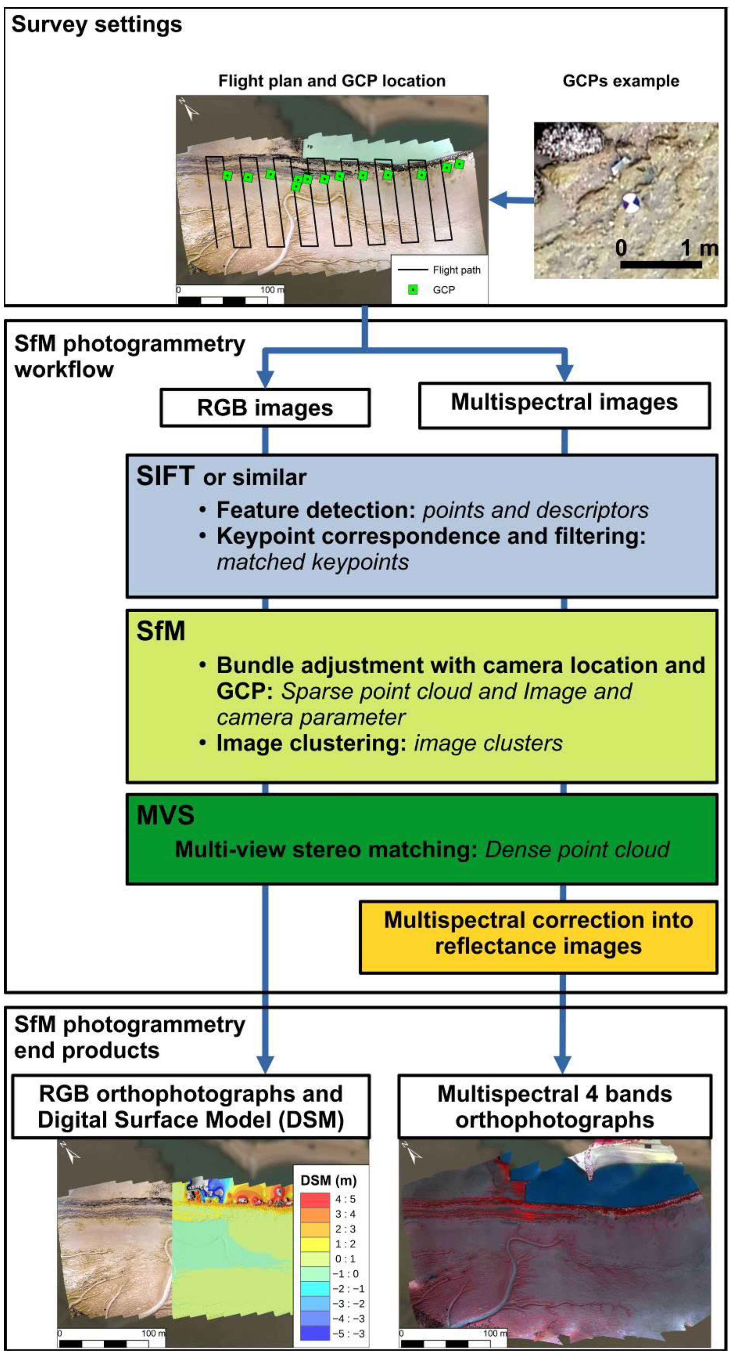
2.2. UAS Survey Setting

The study area (Figure 1C–E) was surveyed using an unmanned aircraft vehicle (UAV), a DJI Phantom 4 v2 equipped with a standard RGB camera, and a simultaneously loaded small-sized Parrot Sequoia+ multispectral camera (Figure 2 and

Table 1. Summary of unmanned aircraft system (UAS) settings for surveying the intertidal mudflat: unmanned aircraft vehicle (UAV), cameras, flight plan, and ground control.

UAV Parameter
UAV model	DJI Phantom 4 Pro
Flight duration	25 min
Flight plan design and piloting software	DJI Ground Station Professional
Cameras parameter
Sensor type	RGB Phantom 4 Pro main camera	Parrot Sequoia+ multispectral camera
Sensor/image size	CMOS 1.2/3″ (20 Megapixel (MP))	1280 × 960 pixels (1.2 Megapixel (MP))
Shutter release	Global shutter	Global shutter
Focal length	8.8/24 mm	3.98 mm
Multispectral bands	-	Green 550 nm (40 nm width) Red 660 nm (40 nm width) Red-edge 735 nm (10 nm width) Near-Infrared 790 nm (40 nm width)
Gimbal	Stabilised over 3 axes (vertical inclination, roll, panoramic)	Rigid gimbal fixed on UAV shoes with a mast to support Sunshine sensor device
Additional features		IMU, GPS, Sunshine sensor (spectral sensors centred on camera spectral bands), ≈20% reflectance panel
Flight plan settings parameters
Image ground size dimension (GSD) pixel	5 cm/pixel (multispectral) 0.5 cm/pixel (RGB)
Flight height	45 m above ground level
Frontal overlap	80%
Lateral overlap	60%
Shooting interval (triggered on time)	2 seconds
Surveyed area	4.95 ha (330 × 150 m)
Ground segment settings parameters
Positioning device	Topcon Hiper SR antenna
Ground control point (GCP) number	13

). Images were acquired on 2 October 2019, during the late seasonal bloom of MPB [5] under cloudy weather and low spring tide conditions (water column height at 0.82 m at 12:04 pm UTC). The flight was conducted one hour before low tide (e.g., ~11:00 am UTC) to observe MPB maximum biomass [13,32].

The DJI Phantom 4 RGB camera was a 20 MP (megapixel) resolution sensor with a 8.8 to 24 mm focal lens, mounted on three axes gimbals. The Sequoia+ multispectral camera was a four monoband global shutter camera with a fixed lens with a resolution of 1.2 MP. Its spectral range included a green (550 nm ± 40 nm), red (660 ± 40 nm), red edge (735 nm ± 10 nm), and near-infrared (790 nm ± 40 nm) bands. The camera system included, in addition, a sunlight sensor (with the same spectral bands as the multispectral camera) combined with an inertial measurement unit (IMU) and GPS devices (Table 1). For more setting details, see Table 1.

The flight plan was designed using the DJI Ground Station Professional application and by taking into account the specificities of the Sequoia+ multispectral camera (i.e., showing the lowest resolution) (Figure 2 and Table 1). This study aimed to provide a very high spatial resolution multispectral orthorectified dataset. Consequently, the ground size dimension (GSD) image pixel was set to 5 cm/pixel for the multispectral camera and 0.5 cm/pixel for the RGB camera. This implied flying at 45 m above ground level over an area of 330 m long-shore × 150 m cross-shore. The camera orientations were set to obtain nadir photographs with a frontal overlap (i.e., frontlap) of 80% and a lateral overlap (i.e., sidelap) of 60% with the multispectral sensor. The shooting interval was triggered at 2s. Radiometric calibration of the camera was operated before and after the flight using a dedicated reflector panel provided by the manufacturer and which was a nearly a 20% reflector panel. The RGB camera was set for the flight with fixed parameters, such as a lens zoom at 8.8 mm and the focus fixed to the infinite (Table 1).

For the flight session, the ground segment included measurements of 13 checkered boards (Figure 2) as ground control points (GCP), which were georeferenced at centimetre accuracy using a differential GPS (DGPS) device with continuous real time kinematic (RTK) positioning correction through networked transport of RTCM via internet protocol (NTRIP).

2.3. Structure from Motion—Multi-View Stereo (SfM-MVS) Photogrammetry Processes

The images were processed using the SfM-MVS photogrammetry method with two softwares: Agisoft Metashape Professional for RGB images and Pix4D Mapper for multispectral images. Both softwares provided a standard SfM-MVS photogrammetry pipeline [26,33,34,35], summarized in Figure 2. The workflow consisted in, first, automatically detecting and tying key points (i.e., points or sets of pixels with distinctive contrast or texture) within the images and across a series of overlapping images through computer vision algorithms such as scale invariant feature transform (SIFT) or its variations. Second, with a sufficient number of images and key points, the SfM process performed the bundle adjustment (i.e., the image alignment) that retrieved and adjusted the location, orientation, and camera parameters of images. The SfM process was aided by image coordinates recorded by the UAV and the GCPs. The result of the SfM step was a sparse cloud point from key points scaled through image and GCPs coordinates. Third, refined image location and camera parameters provided by the SfM process were used in the MVS process to produce a dense point cloud with a density usually equal to twice that of the GSD of the image (i.e., one point for two pixels of image). Surface interpolation was performed over the dense point cloud to produce the digital surface models (DSM). Images were orthorectified and mosaicked over the DSM to produce the orthophotographs with resolution equal to GSD. The 13 GCPs were used to georeference and adjust the SfM bundle adjustment of images and assess the quality of the DSM geometry. Horizontal and vertical accuracy assessment metrics of DSM were provided by Agisoft Metashape, such as mean signed deviation (MSD) and root mean square error (RMSE) of GCP location from field to DSM. During the process, multispectral images were converted into reflectance using simultaneous measurement of incident light by the sunlight sensor, avoiding potential bias due to changes in sunlight during the acquisition [26]. For more details regarding SfM photogrammetry method see [14,19,35].

Orthophotographs and DSM from RGB images were produced with a resolution of, respectively, 0.5 cm and 1 cm per pixel, while those from multispectral images were produced with a pixel resolution of 5 cm and 10 cm. Due to a coarser pixel resolution of the DSM from multispectral images, only RGB images were used for geomorphic analysis.

Finally, to avoid noisy elevation data, especially over water surfaces and along the borders of the DSM (i.e., the bowl effect) due to lack of texture and image overlap or object movement as observed in many other studies such as [20,36,37,38], the noisy data were removed from the DSM by filtering the dense cloud point of water surfaces and suppressing points from the borders.

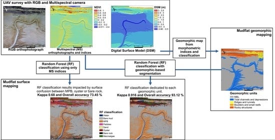
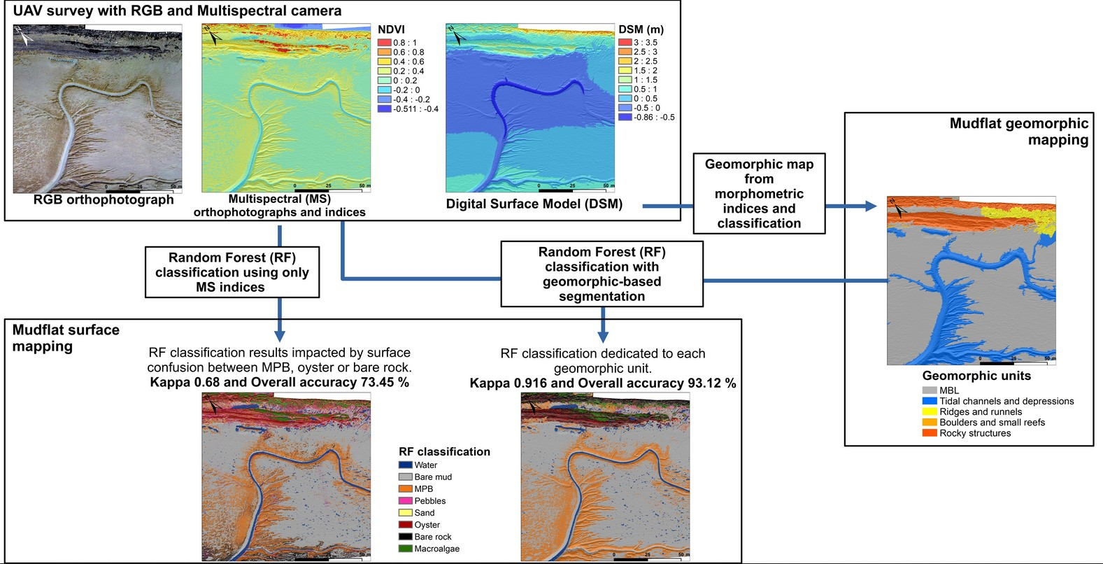
2.4. Image Classifications

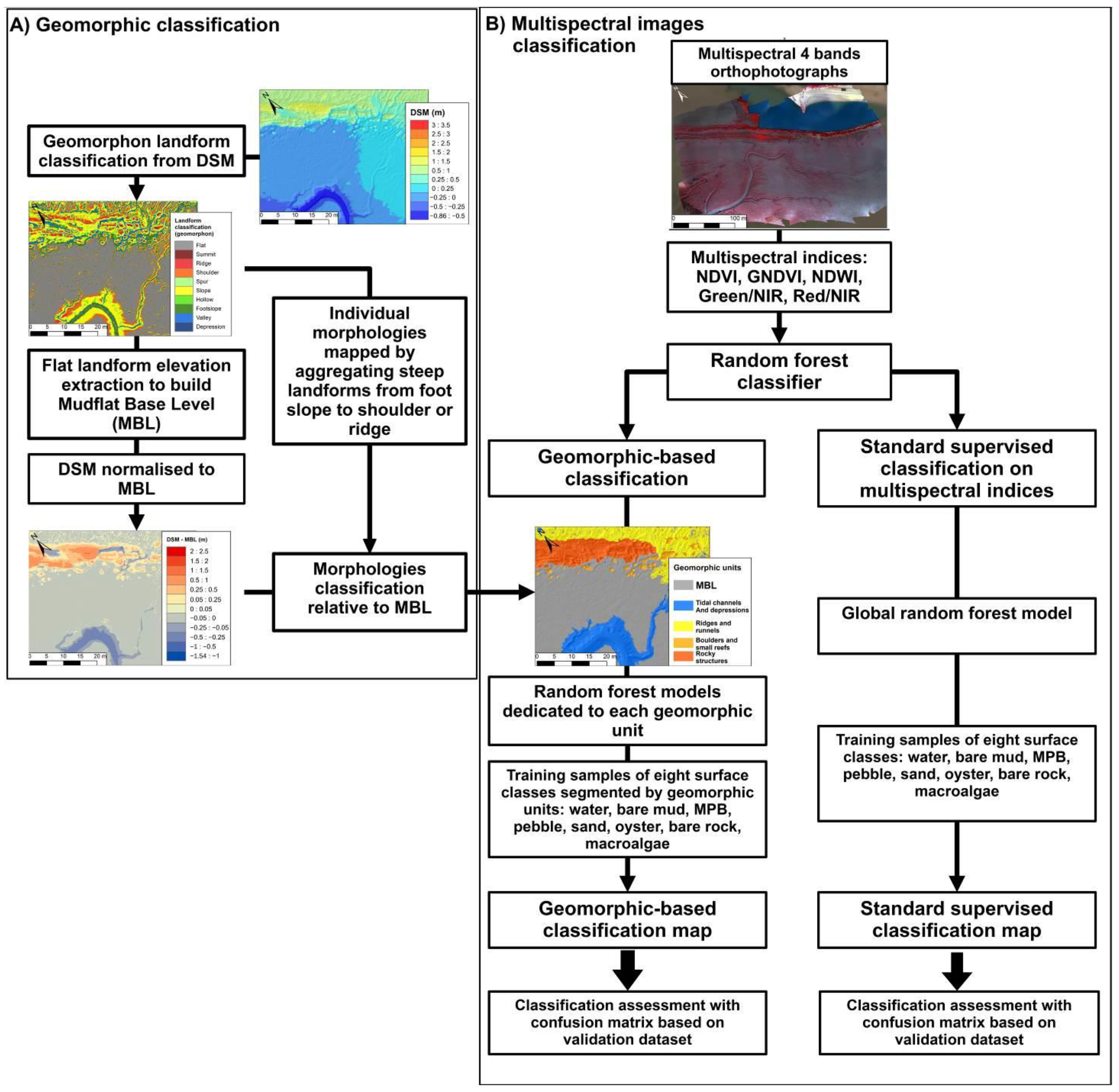
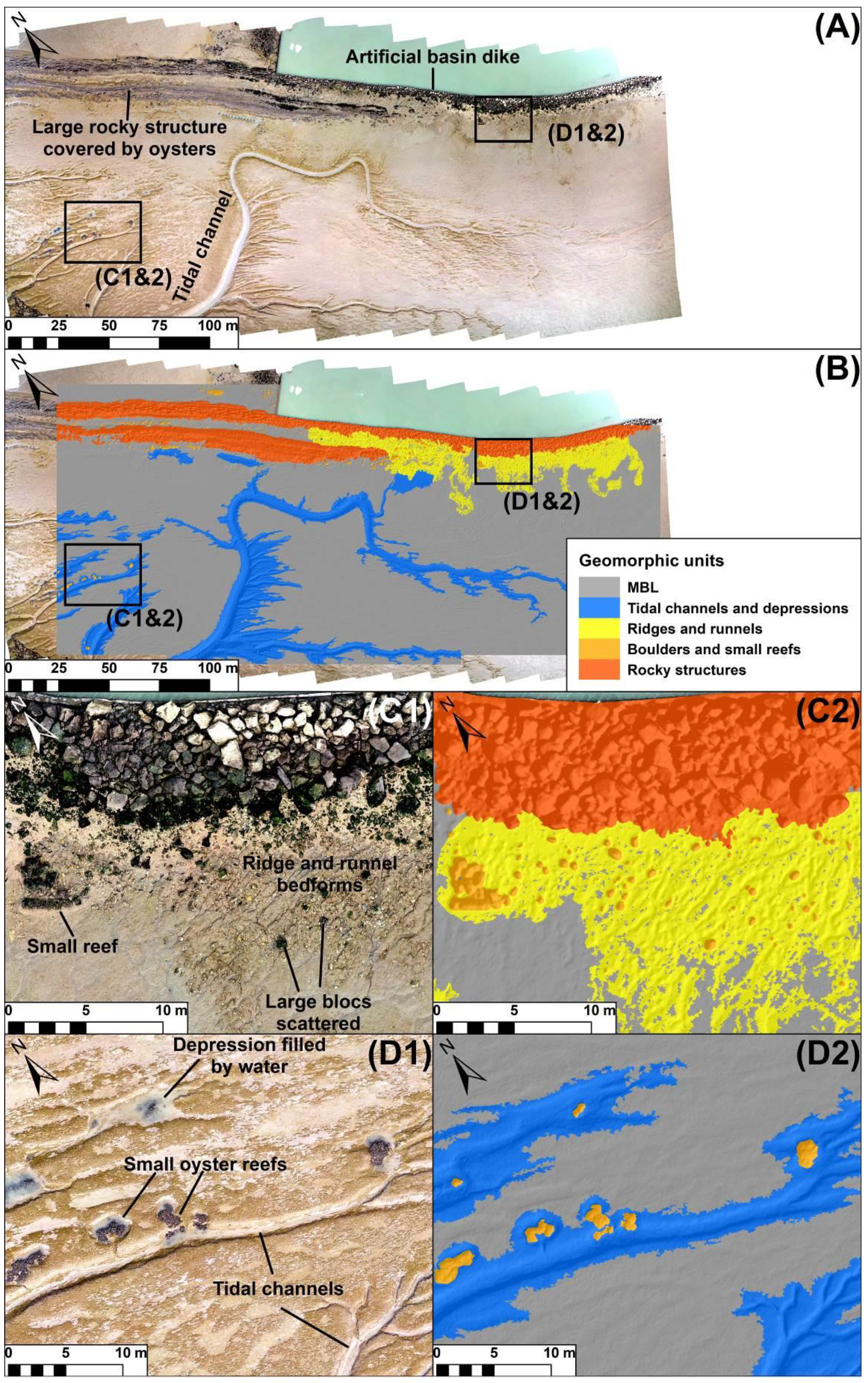
2.4.1. Geomorphological Mapping Method

The main geomorphic units were identified from the DSM (Figure 3A) using the elevation of the top of the mudflat elevation without the principal incised bed forms as a reference, named mudflat base level (MBL) (Figure 3A). The geomorphological mapping was processed following three steps: (1) classifying the elevation dataset in 10 homogeneous landform features (i.e., 10 geomorphons, Figure 3A); (2) defining MBL by extracting flat landform features and normalising DSM elevation to MBL (Figure 3A); (3) clustering steep slope landform features in individual steep morphologies and classifying them regarding their elevation normalised to MBL in five geomorphic units (Figure 3A).

First, due to the topographic diversity of the intertidal flat, the landform units were detected using the “geomorphon” (for geomorphologic phenotype) function [39]. The geomorphon method allowed the classification of DSM cells into 10 types of landforms: flat surface, summit, ridge, shoulder, spur, slope, hollow, valley, depression, and footslope (Figure 3A). This method was based, first, on the image texture similarity concept [40] using the relative elevation of the cell of interest and its neighbours and, second, on a line of sight concept [41] using terrain openness along eight principal compass directions. Thus, geomorphons provided a high degree of terrain autocorrelation [42] detecting transitions between landforms. The geomorphon classification method was set with a radius of 2 m to analyse terrain openness, and the surfaces were considered as flat for slopes below 5°. The radius parameter of 2 m was defined regarding the metric size of mudflat morphologies. This method was used with its current implementation in the system for automated geoscientific analyses (SAGA) free GIS software [43].

Second, the largest flat landform elevation, corresponding to the MBL, was isolated and extrapolated over the entire study area to remove elevation range changes from highest to lowest intertidal area (Figure 3A). This new vertical reference was used to normalise the original DSM elevation to determine if the steep morphologies corresponded to incised (e.g., channels and depressions) or higher-elevation structures (e.g., reefs or boulders). Third, the steep morphologies were mapped by clustering the steep landform features. The geomorphon method provided a high degree of terrain autocorrelation, and the landform features were directly and spatially connected. The succession of steep landforms followed from valley or foot slope to regular slope and, finally, to shoulder or ridge. The clustering step began by converting the landform classification map from image dataset to geometric features in a shapefile. Then, a spatial joint function from GIS software was used to progressively connect valley to foot slope features, then foot slope to regular slope features, and finally regular slope to shoulder or ridges features. Landforms, such as spurs, hollows, or summits, were also aggregated to final steep landforms clusters. Fourth, the morphologies were classified into geomorphic units by considering their position regarding the MBL, estimated by the height or the depth (in m) of each morphology.

Finally, five main geomorphic units were identified over the mudflat: mudflat with very low-lying features, corresponding to the MBL; low incised features at a minimum of 10 cm below the mudflat level, corresponding to the tidal channels and depressions; regular and dense pattern of small channels (10 to 30 cm deep) and ridges (10 to 20 cm high) spaced of 50 cm at least, corresponding to ridges and runnels; isolated boulders or small oyster reefs, exhausted at at least 20 cm above the mudflat level; the rocky area near to the dikes, covered sometimes by oysters or macroalgae (Figure 3B). Manual cleaning by photo-interpretation of the high-resolution orthophotograph from RGB images was performed to ensure the quality of the identification of each of the five geomorphic units.

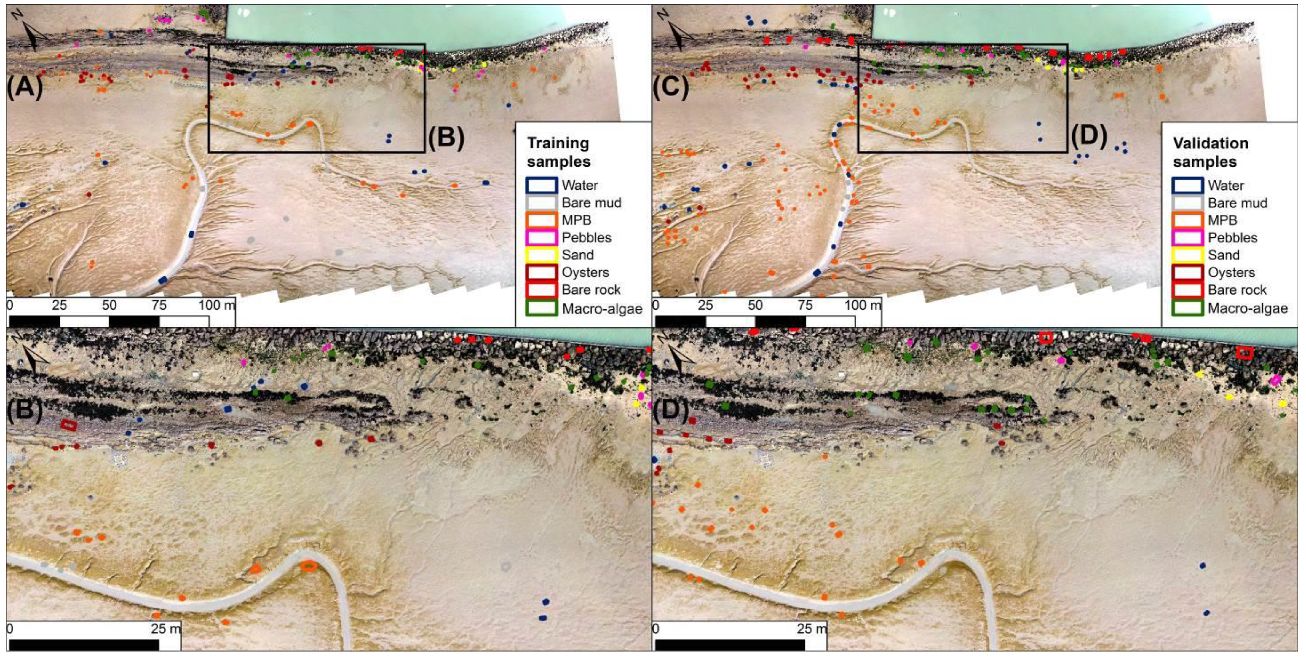
2.4.2. Supervised Image Classification Using Standard and Geomorphic-Based Random Forest Classifier

A random forest classifier (RF) is a machine learning classification combining decision trees and bootstrapping [44]. This method was successfully used for tidal flats [1,15] and benthic vegetation [45]. RF uses supervised classification algorithms, allowing handling of collinearity and non-linearity between predictive variables. Each decision tree was created by using a random sample of predictive data, resampled at each iteration of the algorithm. Then, for each pixel, the final classification was obtained by a majority vote: the final class of a pixel is the class that appeared most of the time at the end of each algorithm iteration. This classification method can be divided into three steps: model building, image classification, and accuracy assessment.

The RF classifier model was created using the “caret” package for R software [46]. Two parameters were set up: the number of trees and the number of selected and tested variables as predictors for the best split when growing the trees. In the current study, the number of trees was set at 500 following [15] recommendations to limit computer calculation time, while not impacting RF result quality. Due to the absence of blue bands within the multispectral images, the predictors used were the normalised difference vegetation index (NDVI), the green-based NDVI (GNDVI), the normalised difference water index (NDWI), and the red and green bands normalised to the NIR band (red/NIR and green/NIR) (Figure 3B). The NDVI, GNDVI, and NDWI formulae are:

$$\mathrm{NDVI}=\left(\mathrm{NIR}-\mathrm{Red}\right)/\left(\mathrm{NIR}+\mathrm{Red}\right)$$

$$\mathrm{GNDVI}=\left(\mathrm{NIR}-\mathrm{Green}\right)/\left(\mathrm{NIR}+\mathrm{Green}\right)$$

$$\mathrm{NDWI}=\left(\mathrm{Green}-\mathrm{NIR}\right)/\left(\mathrm{Green}+\mathrm{NIR}\right)$$

where NIR is the NIR band, red is the red band, and green is the green band.

Eight main types of surfaces were identified and used to train the RF algorithm classification during the model building step: water, bare mud (i.e., without MPB biomass detectable), MPB, pebbles, sand, oyster, macroalgae, (including brown (ochrophytes), green (chlorophytes) and red (rhodophytes), and bare rock (Figure 3B). Pure pixels of each type of surface were selected by photo-interpretation using the high-resolution orthophotograph from RGB and NDVI images and delimited as training sample polygons through GIS software (Figure A1). Several classes may have a similar range of responses with multispectral indices. We evaluated the similarities between classes through statistical analysis with descriptive statistics, such as average and standard deviation and non-parametric Kruskal-Wallis and pairwise Dunn’s tests. The tests were applied to the training samples of classes and for each index.

In order to assess the efficiency of the geomorphic-oriented image classification, a formal methodology of image classification was implemented using a standard RF approach (Figure 3B). The image classification was performed over the whole study area without any geomorphic segmentation. Then, a second RF classification was performed using the prior geomorphic unit segmentation of the mudflat (Figure 3B). The image classification method was then implemented by considering only the surface classes included in each geomorphic unit that are indicated in

Table 2. Summary of training and validation samples by surface classes for standard RF classification and for geomorphic-based RF classification. Training and validation samples are expressed as the number of pixels at the multispectral and indices image resolution (i.e., 5 cm/pixel). The training samples for geomorphic-based RF classification were distinguished by geomorphic unit.

Training samples for Standard RF classification without segmenting the multispectral and indices images
	Class 1: Water	Class 2: Bare mud	Class 3: MPB	Class 4: Pebbles	Class 5: Sand	Class 6: Oysters	Class 7: Bare rock	Class 8: Macro algae
Number of pixels	4105	5371	3771	638	200	2171	666	642
Training samples for Geomorphic-based RF classification
	Class 1: Water	Class 2: Bare mud	Class 3: MPB	Class 4: Pebbles	Class 5: Sand	Class 6: Oysters	Class 7: Bare rock	Class 8: Macro algae
MBL (number of pixel)	580	3922	1032	436	159	-	-	143
Tidal channels and depression (number of pixel)	3143	1025	2372	-	-	-	-	-
Ridges and runnels (number of pixel)	165	318	168	68	41	-	-	62
Boulders and small reefs (number of pixel)	13	77	123	-	-	653	69	241
Rocky structures (number of pixel)	272	91	115	134	-	1518	597	196
Validation samples for both RF classification methods
	Class 1: Water	Class 2: Bare mud	Class 3: MPB	Class 4: Pebbles	Class 5: Sand	Class 6: Oysters	Class 7: Bare rock	Class 8: Macro algae
Number of pixels	4129	858	5592	889	434	3101	10,010	2074

. For example, into channel/depression geomorphic units, MPB, bare mud, and water classes were the only visible classes, while small and large reefs showed more surface class types. The training sample polygons (Figure A1) were then filtered by geomorphic units before training models. The input image dataset (i.e., the predictor dataset) was the one segmented by geomorphic unit (Figure 3B), and a RF model, dedicated to a specific geomorphic unit, was trained and implemented on the segmented image dataset. The results from each geomorphic unit were combined to produce a unique image of the result. The general validation procedure was implemented on the final product image. The RF model and image classification accuracy assessments were made using a standard error matrix operated from SAGA GIS. The RF model accuracy was computed from validation samples independent of the training samples (Figure 3B and Figure A1 and Table 2). Accuracy metrics of image classification were provided, such as user and producer accuracy for each class, overall classification accuracy, and kappa. The user accuracy (in %) essentially describes how often the class on the map will be present on the ground (within the validation polygon), while the producer accuracy (in %) describes how often real features on the ground are correctly shown on the classified map. The kappa metric (unitless) gives an idea of the overall accuracy and the homogeneity of accuracies between surface classes. Overall accuracy (in %) describes, out of all of the validation samples, what proportion was mapped correctly. In addition, a binary agreement and disagreement map between the two classifications was produced by comparing, pixel to pixel, the classification results to highlight where they were similar (agreement between classifications) or different (disagreement)).

3. Results

3.1. Geomorphic Mapping

The SfM-MVS photogrammetry pipeline produced two types of end products from both cameras (Figure 2): (1) an orthophotograph with the same resolution as the GSD selected for the survey (Table 1 and

Table 3. Summary of end-product specifications and accuracy.

Camera Model	Phantom 4 Professional RGB Camera	Parrot Sequoia+ Multispectral Camera
Number of photographs	186	313 per bands (1252 in total)
Coverage area in ha	4.89 ha	7.24 ha
Dense points cloud number and density per m2	73,524,417 points ≈ 1440 points/m2	1,905,290 points ≈ 36.13 points/m2
Orthophotograph resolution in m/pixel	0.0132 m/pixel	0.0504 m/pixel, resampled to 0.05 m/pixel
DSM resolution in m/pixel	0.026 m/pixel, resample to 0.05 m/pixel	0.07 m/pixel, resample to 0.10 m/pixel
Global RMSE accuracy in m from GCPs geolocation	0.03 m	0.02 m

); (2) a model of elevation reproducing the objects visible on photographs in 3D, named DSM. These outputs were provided with accuracy metrics related to the density of cloud points per m² and to the accuracy of the elevation model (Table 3).

The geolocation accuracy of the output from GCPs was very high, with 0.03 and 0.02 m for, respectively, the RGB and multispectral cameras (Table 3).

The geomorphic map displayed classical mudflat landforms (Figure 4). The MBL geomorphic unit covered the overall study area with an elevation ranging between 0 and 0.4 m and a gentle slope of less than 5° of inclination converging towards the tidal channels. This unit represented 70.9% of the study area and corresponded to the large flat landforms (Figure 3 and Figure 4).

The tidal channels and depressions were located southward in the central part of the mudflat and on the western side of the study area. The tidal channels were situated between the bank levee and the bed and had depths of 0.2 m to 0.8 m below MBL and widths of 1 m to 10 m. A major channel was present from the eastern border in the centre of the study area before turning south. Its size and depth increased progressively. Ten less deep tributary tidal channels were connected to this main channel, draining the eastern and central part of the mudflat. Four smaller tidal channels flowed westward from the western part of the study site. The major tidal channel was at this time water-filled, whereas the others were mostly dried up. The external limit of the tidal channel bedforms was contoured using the spatial continuity and connectivity of landform features characterising their bank levees, such as foot slopes, ridges, and shoulder landforms.

Twelve depressions were mapped along with the major reef structures and western tidal channels. These depressions were mostly water-filled and comprised isolated oyster reefs. They were contoured using the landforms describing their banks, such as ridges, shoulders, slope, and foot slope.

The northern border showed a rocky structure corresponding to a recent dike made of large boulders supporting a backshore artificial seawater-filled basin. The dike elevation was 1.5 m above the mudflat surface and was 4 to 6 m-wide. This dike extended westward as an older damaged dike 1 m above the MBL and 5 to 6 m wide and composed of dismantled and breached blocks. Another rocky structure, 12 to 14 m wide, was located alongside and southward of this dike extension at 1 to 1.4 m above the MBL. Theses rocky structures represented 14.3% of the study area. They were distinguished by aggregating the following landforms: foot slopes, slopes, shoulders, ridges, peaks, spurs, and hollows with spatial continuity. The foot slope landforms helped to contour the external borders of these structures.

Numerous isolated boulders and oyster reefs were scattered around these rocky structures and had elevations of 0.3 to 0.6 m above the MBL and widths between 0.4 m and 3 m. They collectively form the “boulders and small reefs” geomorphic unit and represented 0.8% of the study area. The spatial continuity of foot slope, slope, ridge, and shoulder was used to distinguish these structures.

The northern part of the mudflat presented ridge and runnel units extending southward. The ridges were 0.1 to 0.2 m above the MBL and 0.4 to 1 m wide. This unit was mapped using spatial continuity from valley and foot slope landforms to slope and ridge landforms. The valley and foot slope landforms were selected on the basis of their proximity, which was set at less than 1 m.

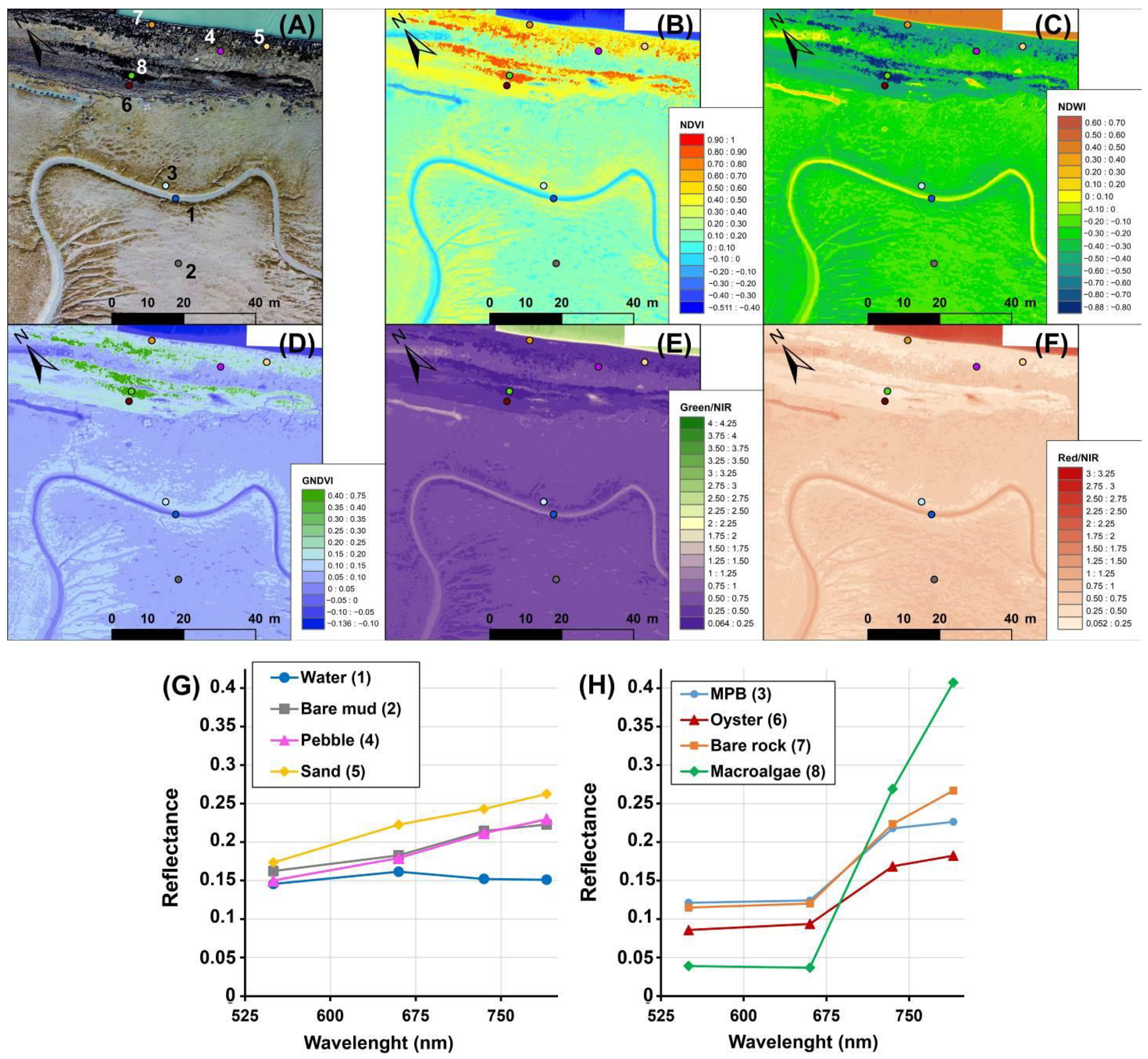
3.2. Reflectance Spectra and Multispectral Indices

Assessment of spectral properties and multispectral indices obtained from mudflat surfaces was conducted from the training and validation samples dataset (Figure 5). The water, bare mud, and macroalgae surface observed on the RGB image (Figure 5A) were also clearly highlighted with a very distinct range of values with the multispectral indices (Figure 5B–F). On the contrary, MPB, pebbles (at the foot slope of the dike), oyster reefs, and bare rock surfaces showed similar ranges of multispectral indices, except the NDWI index (Figure 5C), for which MPB and oysters were more distinct. Typical reflectance spectra of the different surface classes (Figure 5G,H) globally showed a limited spectral contrast due to the low multispectral resolution. In particular, the pebble, oyster, and bare rock classes showed spectral similarity. The pebble spectrum was very close to that of bare mud, except for the green region, which was slightly lower. The oyster spectrum showed a spectral shape similar to the MPB spectrum but with lower reflectance values. The bare rock spectrum was very close to the MPB spectrum in visible and red-edge regions, while the near-infrared region was more reflective.

The similarities and differences between classes were highlighted by analysing their response within multispectral index values averaged over the pixels from training and validation samples (

Table A1. Multispectral index dataset statistics such as mean and standard deviation (i.e., Std) for each surface class used within RF classification.

Multispectral Index	NDVI		NDWI		GNDVI		Green/NIR		Red/NIR
	Mean	Std	Mean	Std	Mean	Std	Mean	Std	Mean	Std
Water	−0.052	0.086	0.020	0.112	−0.001	0.026	1.072	0.279	1.129	0.212
Bare mud	0.137	0.029	−0.185	0.021	0.070	0.010	0.689	0.030	0.760	0.045
MPB	0.362	0.044	−0.356	0.035	0.116	0.013	0.476	0.039	0.470	0.049
Pebbles	0.216	0.106	−0.284	0.076	0.102	0.029	0.564	0.093	0.658	0.145
Sand	0.079	0.013	−0.210	0.018	0.086	0.011	0.654	0.024	0.854	0.023
Oyster	0.386	0.089	−0.423	0.079	0.134	0.045	0.410	0.084	0.449	0.100
Bare rock	0.332	0.081	−0.351	0.075	0.130	0.031	0.485	0.084	0.507	0.095
Macro algae	0.785	0.080	−0.753	0.088	0.279	0.063	0.144	0.063	0.123	0.057

). Water, bare mud, sand, and macroalgae classes were well distinguished with, as an example, a mean NDVI of, respectively, −0.052, 0.137, 0.079, and 0.785 (Kruskal-Wallis, p < 0.01 and Dunn’s post hoc, p < 0.001). MPB, pebbles, oysters, and bare rock were more confused with, as an example, mean values of NDVI of 0.362, 0.216, 0.386, and 0.332, respectively (Dunn’s post hoc, p > 0.05). Moreover, the pebbles, oyster, bare rock, and macroalgae surface classes showed the highest standard deviation values (Table A1), thus indicating that they encompassed a wide range of index responses. These observations were similar to NDWI, GNDVI, green/NIR, and red/NIR indices (Table A1). For all the multispectral indices but NDWI, there were no significant statistical differences between MPB, oyster, and bare rock classes (Kruskal-Wallis, p > 0.05, Table A1). The oyster class showed significant lower NDWI values compared with those of the two other classes (Dunn’s post hoc, p < 0.0001).

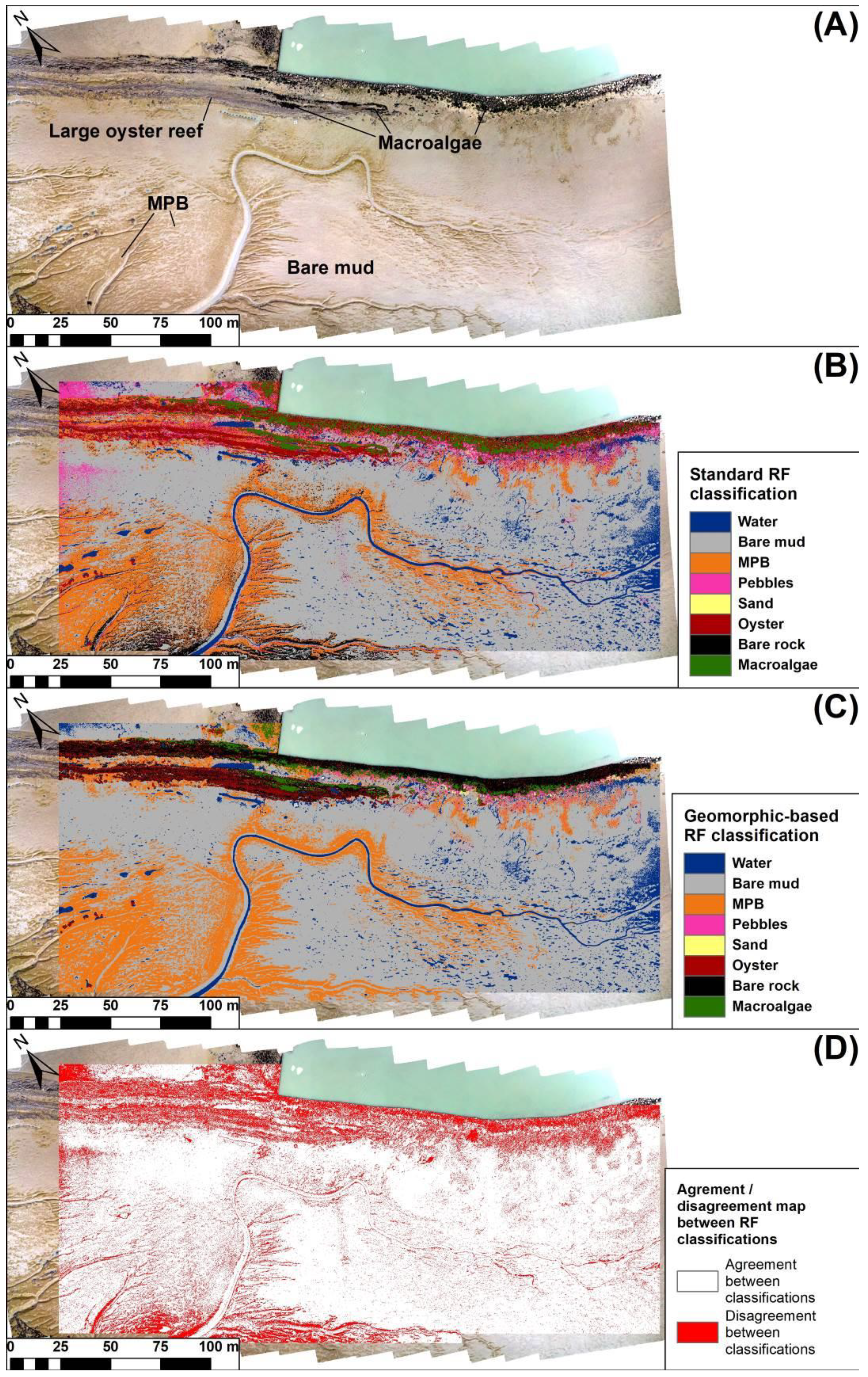
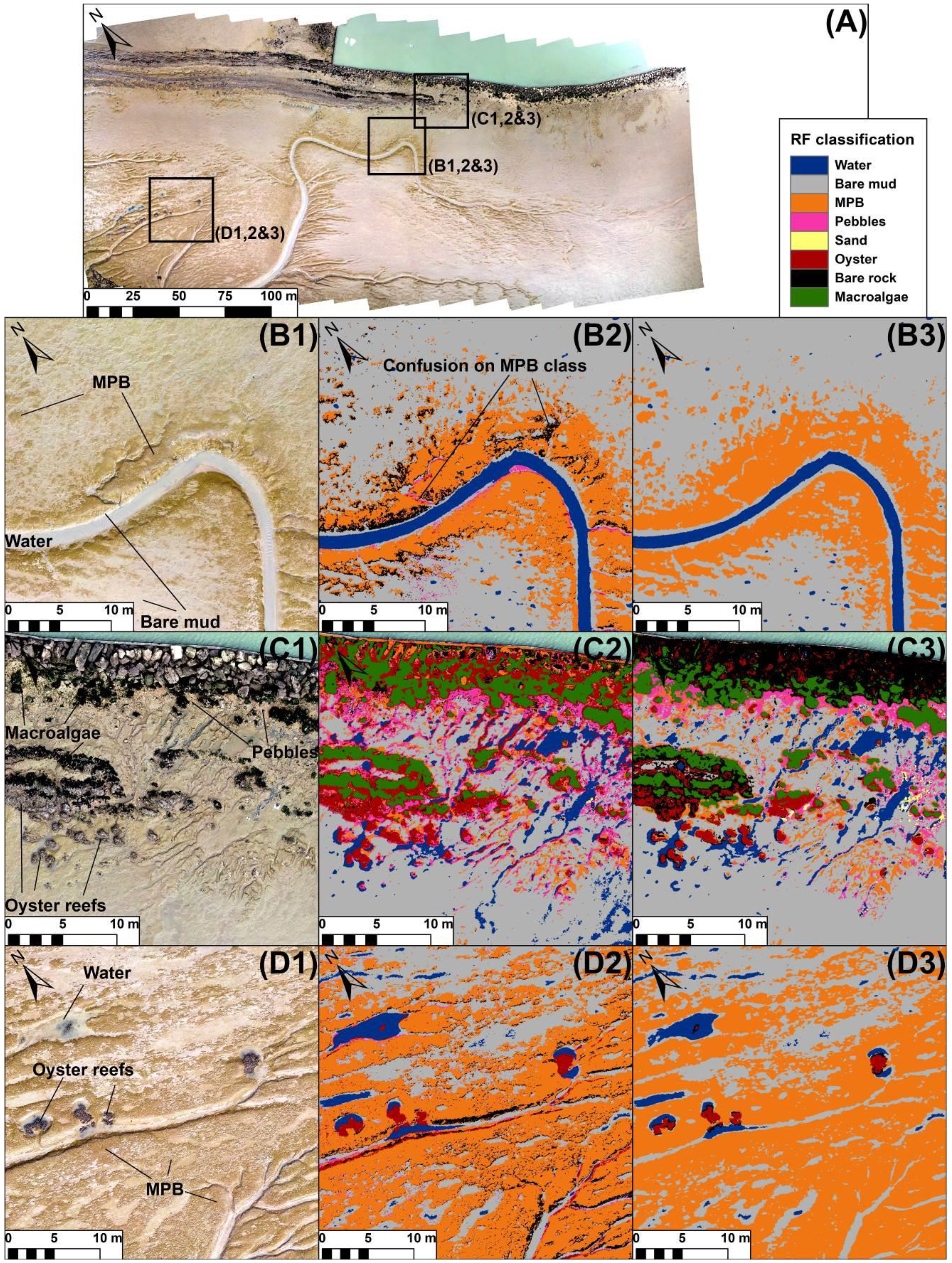
3.3. Standard Image Classification

The image classification was performed on the whole area using training samples materialized by polygons drawn on the eight surface classes (Figure A1 and Table 2). The image classification showed surface class spatial distribution of, respectively, 7.52% for water, 56.22% for bare mud, 18.67% for MPB, 4.69% for pebbles, 0.05% for sand, 5.41% for oyster, 5% for bare rock, and 2.44% for macroalgae (Figure 6 and Figure 7).

Table 4. Standard RF classification confusion matrix and user and producer accuracies. Numbers correspond to the number of pixels of each training polygon (columns) classified within the eight classes (rows). Numbers not on the diagonal correspond to confusion (i.e., not properly classified). The accuracies correspond to the percentage (%) of the total pixel properly classified within the polygons (i.e., user accuracy) or within the classes (i.e., producer accuracy).

	Water	Bare Mud	Mud with MPB	Pebbles	Sand	Oyster	Bare Rock	Macro Algae	Total	User Accuracy in %
Water	7702	20	9	0	0	0	8	0	7739	99.52
Bare mud	713	6209	161	0	0	4	51	4	7142	86.93
Mud with MPB	0	0	8288	0	0	184	646	33	9151	90.56
Pebbles	7	0	245	638	0	243	384	32	1549	41.18.
Sand	0	0	0	0	200	0	0	0	200	100
Oyster	0	0	148	0	0	4996	5114	67	10,325	48.38
Bare rock	0	0	1131	0	0	236	2797	10	4174	67.01
Macro algae	0	0	1	0	0	0	2810	3044	5855	51.98
Total	8422	6229	9983	638	200	5663	11810	3190
Producer accuracy in %	91.45	99.67	83.02	100	100	88.22	23.68	95.42
Overall accuracy in %								73.45
Kappa metric								0.68

presents the confusion matrix and the user and producer accuracies in percent for each surface class. The kappa and overall accuracy metric of this method were, respectively, 0.68 and 73.45% with important disparities regarding classes (Table 4). The producer accuracy was, respectively, 91.45% for water, 99.68% for bare mud, 83.02% for MPB, 100% for pebbles, 100% for sand, 88.22% for oyster, 23.68% for bare rock, and 95.42% for macroalgae. Classification confusion appeared between the MPB class and the bare rock class mainly. This confusion concerned, also, the pebbles class, the bare rock class, and the oyster class, but with limited spatial impact on the tidal channel bedforms (Figure 4 and Figure 6).

3.4. Geomorphic-Based Image Classification

The image classification was made successively on each geomorphic unit, and this included the limitation of the number of surface classes characterising them (Table 2).

Table 5. Geomorphic-based image classification confusion matrix and user and producer accuracies. Numbers correspond to the number of pixels of each training polygon (columns) classified within the eight classes (rows). Numbers not on the diagonal correspond to confusion (i.e., not properly classified). The accuracies correspond to the percentage (%) of the total pixel properly classified within the polygons (i.e., user accuracy) or within the classes (i.e., producer accuracy).

	Water	Bare Mud	Mud with MPB	Pebbles	Sand	Oyster	Bare Rock	Macro Algae	Total	User Accuracy in %
Water	7843	0	6	19	0	1	2	0	7871	99.64
Bare mud	756	6285	220	233	172	121	4	15	7806	80.51
Mud with MPB	0	2	9780	38	0	332	1	70	10,223	95.66
Pebbles	0	0	150	202	0	0	0	4	356	56.74
Sand	0	0	0	0	41	0	0	0	41	100
Oyster	0	0	0	164	0	5092	176	1	5433	93.72
Bare rock	0	0	0	3	0	194	11,736	33	11,966	98.07
Macro algae	0	0	0	0	0	0	36	3112	3148	98.85
Total	8599	6287	10,645	659	213	5740	11,970	3235
Producer accuracy in %	91.20	99.96	91.87	30.65	19.24	88.71	98.04	96.19
Overall accuracy in %								93.12
Kappa metric								0.916

presents the confusion matrix and the user and producer accuracies. The kappa and the overall accuracy metric of the geomorphic-based image classification were, respectively, 0.916 and 93.12%, with some disparities regarding pebble, sand, and oyster (Table 5). The producer accuracy was, respectively, 91.2% for water, 99.96% for bare mud, 91.9% for MPB, 30.65% for pebble, 19.25% for sand, 88.71% for oyster, 98.04% for bare rock, and 96.19% for macroalgae. The class confusion concerned mainly those with very limited spatial coverage, such as pebble and sand (Figure 6 and Figure 7). Detailed analysis of these disparities was provided regarding each surface class.

The classes over the whole area represented, respectively, 6.8% for water, 61.15% for bare mud, 21.32% for MPB, 0.87% for pebble, 0.16% for sand, 2.5% for oyster, 5.39% for bare rock, and 1.76% for macroalgae (Figure 6 and Figure 7). The water surfaces were located mostly in the talweg of tidal channels and depressions. Thin water bodies detected over the mudflat unit corresponded to small ponds created by low-lying drainage morphologies (a few centimetres in height) that were undetected with the DSM resolution. The bare mud surfaces were observed in the inner part of the mudflat unit a few metres from tidal channels, depressions, or rocky structures. The drainage morphologies showed almost exclusively bare mud surfaces, such as the lower part of tidal channel banks and runnels. The MPB surfaces appeared along the upper part of drainage morphologies, such as tidal channel banks or ridges morphologies. MPB propagated a few meters from drainage morphologies to the inner part of the mudflat. MPB was seen, also, on mud deposits at the foot slope of rocky structures colonised by oysters. Pebbles and sand surfaces were observed at the foot slope of major rocky structures, such as the northern dikes. The oyster surfaces were detected, along with major rocky structures, in the northwest of the study area and in small reefs in the southwest. Bare-rock surfaces were detected exclusively on the rocky structures of the northern dikes, especially on the modern dike. The macroalgae colonized mainly the lower part of major rocky structures that were flooded by tides, as well as small rock blocks close to the dikes.

4. Discussion

The objective of mapping mudflat heterogeneous and complex surfaces was reached through the development of a new method combining radiometric and geomorphic data in order to distinguish structures with close spectral signatures and low-lying morphologies. Three interconnected elements were crucial to implementing this method: a high spatial resolution, the use of the DSM, and a prior geomorphic segmentation of the images before the machine learning classification.

4.1. Geomorphological Analysis

The method proposed in this study is highly dependent on the use of the DSM and its spatial resolution. Exploiting DSM information is still not very common for mapping intertidal areas, with only a few previous studies applied to intertidal oyster and polychaete reefs [14,24,47]. Low-lying morphologies, such as ridges and runnels, could be detected at the high spatial resolution of 5 cm/pixel. These structures were identified on the DSM and classified with the geomorphon landforms algorithm [39]. This method analyses landform patterns estimated from the relative height of a DSM pixel compared to its neighbour within eight directions. It is spatially conservative, as a landform class is assigned to pixels without changing topographic parameters. Consequently, the landform classes come in successions without gaps. The geomorphic units were based on the landform classes obtained from the geomorphon classification, further aggregated with a simple spatial joint function from any GIS software. Geomorphic units could have been mapped with other methods based on slope, pixel area, or considering slope and elevation, and by applying metrics such as the topographic position index [48] or topographic openness [41]. However, these latter methods are more adapted to map objects showing marked changes in slope, such as reefs with steep three-dimensional structures, but do not accurately discriminate low-lying morphologies typical of mudflats. A GEOBIA approach would offer another solution to map mudflats by providing a partitioning of the image based on texture, object shape, and the contextual relationship between objects. This technique was successfully used to map intertidal environments [22,24], but the segmentation patterns can be different between two runs. Moreover, setting up the GEOBIA approach requires more expert knowledge compared to the method proposed in this study. This approach can be implemented with free GIS software and only requires basic knowledge in geomorphology to interpret the morphologies on the orthophotograph and the DSM. It can be easily applied to similar ecosystems, such as wetlands or peat-lands, with minor local tuning such as defining the MBL and the thresholds to extract low-lying morphologies, making it highly accessible for operational applications.

4.2. Spectral Constraints

In addition to being composed of low-elevation landforms, mudflat surface classes were also characterized by the similarity of their spectral shapes, in particular with a multispectral resolution. All the multispectral indices used in this study (NDVI, GNDVI, NDWI, green/NIR, and red/NIR) showed significant overlap. As an example, oyster reefs, pebbles, some of the bare rock surfaces, and MPB shared close NDVI values, ranging from 0.2 to 0.4 (Figure 5). The consequence was the difficulty of applying any classification method, including machine learning techniques, due to high confusion and low accuracy. Confusion between MPB and oysters or bare rock appeared especially for channel banks where MPB showed high NDVI values up to 0.4. The confusion also likely arose from the presence of diatoms on oyster shells [23,24] or from rocky surfaces colonised by macro- or microalgae [49]. To overcome these spectral constraints, the geomorphic-based RF classification method provided a geomorphic context to better discriminate the different surface classes. The kappa coefficient and overall accuracy of the classification increased consequently from, respectively, 0.68 and 73.45% for standard RF classification to 0.916 and 93.12% for geomorphic-based RF classification. This accuracy was also higher than that reported in studies from similar intertidal areas. A GEOBIA approach using RGB image and DSM from a UAV survey indicated an overall accuracy of 78.92% and a kappa of 0.72 [19]. The study from [50], based on a multispectral survey and support vector machine (SVM) classification, reported an overall accuracy of 85.03% and a kappa of 0.73. The improved results of the geomorphic-based RF classification can be explained by the lower confusion between MPB and others classes, such as oysters, bare rock, pebbles in channels, depressions, and mudflat units (Figure 5 and Figure 6). Confusion between bare rock, MPB, and oysters on the dike were also drastically reduced (Figure 6). The main improvements were for MPB and bare rock, which covered a large part of the study area and can be explained by the lower number of classes per geomorphic unit. Channel morphologies were only characterized by water, bare mud, and MPB surfaces (Table 2), with a distinct reflectance spectrum (Figure 5) and multispectral index values (Table A1). Channels, depressions, and MBL units represented the largest footprint of the study area and, by avoiding confusion for these areas, the classification accuracy was increased significantly (Table 4 and Table 5). However, pebble and sand classes were still confounded with MPB and ridges and runnels units. This was partly due to their limited spatial coverage that induced an under-representation of these specific classes within the training samples used to build the RF model compared to the over-representation of the MPB class.

4.3. Generalisation of the Method

The methodology proposed in this work exploited the UAV’s very high spatial resolution. Mapping mudflat geomorphic units was possible with a DSM having a centimetre resolution to detect low-lying morphologies, such as ridges and runnels or small reefs. The possibility to still detect these geomorphic features with a decimetre resolution remains to be investigated. The upscaling of the method using satellite data is technically feasible for those having a stereo acquisition [51]. Solutions, such as stereo-satellite image surveys with flexibles sensors such as Pleiades and Pleiades Neo, can cover very large surfaces, thus acquiring topographic and multispectral information. This type of sensor was successfully used to study beach dynamics and coastal landscapes [52,53]. However, DSMs retrieved from satellite images have a 50 to 70 cm pixel resolution that may be too coarse to map mudflat or reef morphologies. Moreover, satellite multispectral images generally have a low multispectral resolution that leads to increasing spectral mixing issues. This problem is reduced at the very high spatial resolution of UAV images. Spectral mixing due to a low spectral resolution can also be partly overcome with UAVs mounted with hyperspectral cameras in the visible and NIR spectral range [54]. However, this type of device is costlier than a multispectral sensor. Even though UAVs have a lower synoptic capacity than satellites, the method proposed in this work, combining topographic and multispectral coverage, can be applied to large mudflat areas. UAVs have different flying capacities but, as an order of magnitude, a minimum of 20 ha covered per flight hour at an altitude of 100 m can be expected. Recent developments in UAV systems, such as the DJI Phantom 4 Multispectral that functions with GNSS RTK or NTRIP corrections, can increase the spatial coverage while keeping a centimetre range pixel resolution [14]. A combination of sensors, such as UAV-based LiDAR coupled to a multispectral camera, can be another solution to obtain topographic and multispectral information over large mudflats [55].

5. Conclusions

A geomorphic segmentation prior to pixel-based classification improved the mapping accuracy of an intertidal mudflat colonized by MPB. Due to the low spectral resolution of the camera, MPB showed similar spectral responses with oyster reefs and rocky areas (the surfaces of which were colonized by photosynthetic organisms). It was, therefore, challenging to identify MPB even with a machine learning technique. We developed a new method that applied a machine learning image classification over geomorphic units. By limiting the number of surface classes within each geomorphic unit, a geomorphic-based RF classification showed an improved overall accuracy higher than 90%. Geomorphic-based classification also provided complementary information for biologists by adding a geomorphological characterisation and quantification of intertidal habitats. MPB was found to colonize tidal channels and depressions. Future studies exploiting the DSM topography could investigate the relationships between MPB and the tidal channel networks at a larger scale. DSM topography may be used to monitor hydrodynamic parameters relevant for the biota, such as flooding duration [20], or to assess the topographic limit of soft-bottom intertidal vegetation, which can be related to mudflat accretion or erosion. By informing on the links between the biology and its physical environment at a high spatial resolution, this method might finally improve our understanding of biological processes that can change with the spatial scale of observation [56]. With their flexibility and low cost, UAVs offer a complementary approach to satellite remote sensing to monitor biological and geomorphic changes in intertidal habitats in response to climate change and anthropogenic pressures.

References

1. Murray, N.J.; Phinn, S.R.; DeWitt, M.; Ferrari, R.; Johnston, R.; Lyons, M.B.; Clinton, N.; Thau, D.; Fuller, R.A. The global distribution and trajectory of tidal flats. Nature 2019, 565, 222–225. [Google Scholar] [CrossRef] [PubMed]
2. Lebreton, B.; Rivaud, A.; Picot, L.; Prévost, B.; Barillé, L.; Sauzeau, T.; Beseres Pollack, J.; Lavaud, J. From ecological relevance of the ecosystem services concept to its socio-political use. The case study of intertidal bare mudflats in the Marennes-Oléron Bay, France. Ocean Coast. Manag. 2019, 172, 41–54. [Google Scholar] [CrossRef]
3. Lovelock, C.E.; Duarte, C.M. Dimensions of blue carbon and emerging perspectives. Biol. Lett. 2019, 15, 20180781. [Google Scholar] [CrossRef] [PubMed]
4. Underwood, G.J.C.; Kromkamp, J. Primary Production by Phytoplankton and Microphytobenthos in Estuaries. Adv. Ecol. Res. 1999, 29, 93–153. [Google Scholar] [CrossRef]
5. Méléder, V.; Savelli, R.; Barnett, A.; Polsenaere, P.; Gernez, P.; Cugier, P.; Lerouxel, A.; Le Bris, A.; Dupuy, C.; Le Fouest, V.; et al. Mapping the Intertidal Microphytobenthos Gross Primary Production Part I: Coupling Multispectral Remote Sensing and Physical Modeling. Front. Mar. Sci. 2020, 7, 520. [Google Scholar] [CrossRef]
6. Legge, O.; Johnson, M.; Hicks, N.; Jickells, T.; Diesing, M.; Aldridge, J.; Andrews, J.; Artioli, Y.; Bakker, D.C.E.; Burrows, M.T.; et al. Carbon on the Northwest European Shelf: Contemporary Budget and Future Influences. Front. Mar. Sci. 2020, 7, 143. [Google Scholar] [CrossRef] [Green Version]
7. Waltham, N.J.; Elliott, M.; Lee, S.Y.; Lovelock, C.; Duarte, C.M.; Buelow, C.; Simenstad, C.; Nagelkerken, I.; Claassens, L.; Wen, C.K.C.; et al. UN Decade on Ecosystem Restoration 2021–2030—What Chance for Success in Restoring Coastal Ecosystems? Front. Mar. Sci. 2020, 7, 71. [Google Scholar] [CrossRef] [Green Version]
8. Barranguet, C.; Kromkamp, J. Estimating primary production rates from photosynthetic electron transport in estuarine microphytobenthos. Mar. Ecol. Prog. Ser. 2000, 204, 39–52. [Google Scholar] [CrossRef] [Green Version]
9. Barnett, A.; Méléder, V.; Blommaert, L.; Lepetit, B.; Gaudin, P.; Vyverman, W.; Sabbe, K.; Dupuy, C.; Lavaud, J. Growth form defines physiological photoprotective capacity in intertidal benthic diatoms. ISME J. 2015, 9, 32–45. [Google Scholar] [CrossRef] [Green Version]
10. Daggers, T.D.; Kromkamp, J.C.; Herman, P.M.J.; van der Wal, D. A model to assess microphytobenthic primary production in tidal systems using satellite remote sensing. Remote Sens. Environ. 2018, 211, 129–145. [Google Scholar] [CrossRef]
11. Launeau, P.; Méléder, V.; Verpoorter, C.; Barillé, L.; Kazemipour-Ricci, F.; Giraud, M.; Jesus, B.; Le Menn, E. Microphytobenthos Biomass and Diversity Mapping at Different Spatial Scales with a Hyperspectral Optical Model. Remote Sens. 2018, 10, 716. [Google Scholar] [CrossRef] [Green Version]
12. Méléder, V.; Rincé, Y.; Barillé, L.; Gaudin, P.; Rosa, P. Spatiotemporal changes in microphytobenthos assemblages in a macrotidal flat (Bourgneuf Bay, France). J. Phycol. 2007, 43, 1177–1190. [Google Scholar] [CrossRef]
13. Echappé, C.; Gernez, P.; Méléder, V.; Jesus, B.; Cognie, B.; Decottignies, P.; Sabbe, K.; Barillé, L. Satellite remote sensing reveals a positive impact of living oyster reefs on microalgal biofilm development. Biogeosciences 2018, 15, 905–918. [Google Scholar] [CrossRef] [Green Version]
14. Brunier, G.; Oiry, S.; Gruet, Y.; Dubois, S.F.; Barillé, L. Topographic Analysis of Intertidal Polychaete Reefs (Sabellaria alveolata) at a Very High Spatial Resolution. Remote Sens. 2022, 14, 307. [Google Scholar] [CrossRef]
15. Oiry, S.; Barillé, L. Using sentinel-2 satellite imagery to develop microphytobenthos-based water quality indices in estuaries. Ecol. Indic. 2021, 121, 107184. [Google Scholar] [CrossRef]
16. Combe, J.; Launeau, P.; Barille, L.; Sotin, C. Mapping microphytobenthos biomass by non-linear inversion of visible-infrared hyperspectral images. Remote Sens. Environ. 2005, 98, 371–387. [Google Scholar] [CrossRef]
17. Harishidayat, D.; Al-Shuhail, A.; Randazzo, G.; Lanza, S.; Muzirafuti, A. Reconstruction of Land and Marine Features by Seismic and Surface Geomorphology Techniques. Appl. Sci. 2022, 12, 9611. [Google Scholar] [CrossRef]
18. Gkiatas, G.T.; Koutalakis, P.D.; Kasapidis, I.K.; Iakovoglou, V.; Zaimes, G.N. Monitoring and Quantifying the Fluvio-Geomorphological Changes in a Torrent Channel Using Images from Unmanned Aerial Vehicles. Hydrology 2022, 9, 184. [Google Scholar] [CrossRef]
19. Brunier, G.; Fleury, J.; Anthony, E.J.E.J.; Gardel, A.; Dussouillez, P. Close-range airborne Structure-from-Motion Photogrammetry for high-resolution beach morphometric surveys: Examples from an embayed rotating beach. Geomorphology 2016, 261, 76–88. [Google Scholar] [CrossRef]
20. Brunier, G.; Michaud, E.; Fleury, J.; Anthony, E.J.; Morvan, S.; Gardel, A. Assessing the relationship between macro-faunal burrowing activity and mudflat geomorphology from UAV-based Structure-from-Motion photogrammetry. Remote Sens. Environ. 2020, 241, 111717. [Google Scholar] [CrossRef]
21. Sedrati, M.; Morales, J.A.; El M’rini, A.; Anthony, E.J.; Bulot, G.; Le Gall, R.; Tadibaght, A. Using UAV and Structure-From-Motion Photogrammetry for the Detection of Boulder Movement by Storms on a Rocky Shore Platform in Laghdira, Northwest Morocco. Remote Sens. 2022, 14, 4102. [Google Scholar] [CrossRef]
22. Duffy, J.P.; Pratt, L.; Anderson, K.; Land, P.E.; Shutler, J.D. Spatial assessment of intertidal seagrass meadows using optical imaging systems and a lightweight drone. Estuar. Coast. Shelf Sci. 2018, 200, 169–180. [Google Scholar] [CrossRef]
23. Román, A.; Tovar-Sánchez, A.; Olivé, I.; Navarro, G. Using a UAV-Mounted Multispectral Camera for the Monitoring of Marine Macrophytes. Front. Mar. Sci. 2021, 8, 1225. [Google Scholar] [CrossRef]
24. Espriella, M.C.; Lecours, V.; Frederick, P.C.; Camp, E.V.; Wilkinson, B. Quantifying intertidal habitat relative coverage in a Florida estuary using UAS imagery and GEOBIA. Remote Sens. 2020, 12, 677. [Google Scholar] [CrossRef] [Green Version]
25. Castellanos-Galindo, G.A.; Casella, E.; Mejía-Rentería, J.C.; Rovere, A. Habitat mapping of remote coasts: Evaluating the usefulness of lightweight unmanned aerial vehicles for conservation and monitoring. Biol. Conserv. 2019, 239, 108282. [Google Scholar] [CrossRef]
26. Collin, A.; Dubois, S.; James, D.; Houet, T. Improving intertidal reef mapping using UAV surface, red edge, and near-infrared data. Drones 2019, 3, 67. [Google Scholar] [CrossRef] [Green Version]
27. Curd, A.; Cordier, C.; Firth, L.B.; Bush, L.; Gruet, Y.; Le Mao, P.; Blaze, J.A.; Board, C.; Bordeyne, F.; Burrows, M.T.; et al. A broad-scale long-term dataset of Sabellaria alveolata distribution and abundance curated through the REEHAB (REEf HABitat) Project 2020. Seanoe 2020, 2. Available online: https://www.seanoe.org/ (accessed on 13 November 2022). [CrossRef]
28. Barillé, L.; Le Bris, A.; Méléder, V.; Launeau, P.; Robin, M.; Louvrou, I.; Ribeiro, L. Photosynthetic epibionts and endobionts of Pacific oyster shells from oyster reefs in rocky versus mudflat shores. PLoS ONE 2017, 12, e0185187. [Google Scholar] [CrossRef]
29. Le Bris, A.; Rosa, P.; Lerouxel, A.; Cognie, B.; Gernez, P.; Launeau, P.; Robin, M.; Barillé, L. Hyperspectral remote sensing of wild oyster reefs. Estuar. Coast. Shelf Sci. 2016, 172, 1–12. [Google Scholar] [CrossRef]
30. Bocher, P.; Piersma, T.; Dekinga, A.; Kraan, C.; Yates, M.G.; Guyot, T.; Folmer, E.O.; Radenac, G. Site- and species-specific distribution patterns of molluscs at five intertidal soft-sediment areas in northwest Europe during a single winter. Mar. Biol. 2007, 151, 577–594. [Google Scholar] [CrossRef]
31. Le Hir, P.; Roberts, W.; Cazaillet, O.; Christie, M.; Bassoullet, P.; Bacher, C. Characterization of intertidal flat hydrodynamics. Cont. Shelf Res. 2000, 20, 1433–1459. [Google Scholar] [CrossRef] [Green Version]
32. Méléder, V.; Barillé, L.; Launeau, P.; Carrère, V.; Rincé, Y. Spectrometric constraint in analysis of benthic diatom biomass using monospecific cultures. Remote Sens. Environ. 2003, 88, 386–400. [Google Scholar] [CrossRef]
33. Lucieer, A.; de Jong, S.M.; Turner, D. Mapping landslide displacements using Structure from Motion (SfM) and image correlation of multi-temporal UAV photography. Prog. Phys. Geogr. 2014, 38, 97–116. [Google Scholar] [CrossRef]
34. Turner, D.; Lucieer, A.; Wallace, L. Direct georeferencing of ultrahigh-resolution UAV imagery. IEEE Trans. Geosci. Remote Sens. 2014, 52, 2738–2745. [Google Scholar] [CrossRef]
35. Iglhaut, J.; Cabo, C.; Puliti, S.; Piermattei, L.; O’Connor, J.; Rosette, J. Structure from Motion Photogrammetry in Forestry: A Review. Curr. For. Rep. 2019, 5, 155–168. [Google Scholar] [CrossRef] [Green Version]
36. Gonçalves, J.A.; Henriques, R. UAV photogrammetry for topographic monitoring of coastal areas. ISPRS J. Photogramm. Remote Sens. 2015, 104, 101–111. [Google Scholar] [CrossRef]
37. Jaud, M.; Grasso, F.; Le Dantec, N.; Verney, R.; Delacourt, C.; Ammann, J.; Deloffre, J.; Grandjean, P. Potential of UAVs for Monitoring Mudflat Morphodynamics (Application to the Seine Estuary, France). ISPRS Int. J. Geo-Inf. 2016, 5, 50. [Google Scholar] [CrossRef] [Green Version]
38. Ouédraogo, M.M.; Degré, A.; Debouche, C.; Lisein, J. The evaluation of unmanned aerial system-based photogrammetry and terrestrial laser scanning to generate DEMs of agricultural watersheds. Geomorphology 2014, 214, 339–355. [Google Scholar] [CrossRef]
39. Jasiewicz, J.; Stepinski, T.F. Geomorphons-a pattern recognition approach to classification and mapping of landforms. Geomorphology 2013, 182, 147–156. [Google Scholar] [CrossRef]
40. Liao, W.H. Region description using extended local ternary patterns. In Proceedings of the International Conference on Pattern Recognition, Istanbul, Turkey, 23–26 August 2010; IEEE: New York, NY, USA, 2010; pp. 1003–1006. [Google Scholar]
41. Yokoyama, R.; Shirasawa, M.; Pike, R.J. Visualizing topography by openness: A new application of image processing to digital elevation models. Photogramm. Eng. Remote Sens. 2002, 68, 257–265. [Google Scholar]
42. Fisher, P. Improved modeling of elevation error with Geostatistics. Geoinformatica 1998, 2, 215–233. [Google Scholar] [CrossRef]
43. Conrad, O.; Bechtel, B.; Bock, M.; Dietrich, H. System for Automated Geoscientific Analyses (SAGA) v. 2.1.4. Geosci. Model Dev. Discuss. 2015, 8, 2271–2312. [Google Scholar] [CrossRef] [Green Version]
44. Breiman, L. Random forests. Mach. Learn. 2001, 45, 5–32. [Google Scholar] [CrossRef] [Green Version]
45. Traganos, D.; Reinartz, P. Machine learning-based retrieval of benthic reflectance and Posidonia oceanica seagrass extent using a semi-analytical inversion of Sentinel-2 satellite data. Int. J. Remote Sens. 2018, 39, 9428–9452. [Google Scholar] [CrossRef]
46. Kuhn, M. Building predictive models in R using the caret package. J. Stat. Softw. 2008, 28, 1–26. [Google Scholar] [CrossRef] [Green Version]
47. Windle, A.E.; Poulin, S.K.; Johnston, D.W.; Ridge, J.T. Rapid and accurate monitoring of intertidal Oyster Reef Habitat using unoccupied aircraft systems and structure from motion. Remote Sens. 2019, 11, 2394. [Google Scholar] [CrossRef] [Green Version]
48. Guisan, A.; Weiss, S.B.; Weiss, A.D. GLM versus CCA Spatial Modeling of Plant Species Distribution Author(s): Reviewed work(s): GLM versus CCA spatial modeling of plant species distribution. Plant Ecol. 1999, 143, 107–122. [Google Scholar] [CrossRef]
49. Meleder, V.; Launeau, P.; Barille, L.; Rince, Y. Microphytobenthos assemblage mapping by spatial visible-infrared remote sensing in a shellfish ecosystem. Comptes Rendus Biol. 2003, 326, 377–389. [Google Scholar] [CrossRef]
50. Chand, S.; Bollard, B. Low altitude spatial assessment and monitoring of intertidal seagrass meadows beyond the visible spectrum using a remotely piloted aircraft system. Estuar. Coast. Shelf Sci. 2021, 255, 107299. [Google Scholar] [CrossRef]
51. James, D.; Collin, A.; Mury, A.; Costa, S. Very high resolution land use and land cover mapping using Pleiades-1 stereo imagery and machine learning. Int. Arch. Photogramm. Remote Sens. Spat. Inf. Sci.-ISPRS Arch. 2020, 43, 675–682. [Google Scholar] [CrossRef]
52. Almeida, L.P.; Almar, R.; Bergsma, E.W.J.; Berthier, E.; Baptista, P.; Garel, E.; Dada, O.A.; Alves, B. Deriving high spatial-resolution coastal topography from sub-meter satellite stereo imagery. Remote Sens. 2019, 11, 590. [Google Scholar] [CrossRef]
53. James, D.; Collin, A.; Mury, A.; Qin, R. Satellite–Derived Topography and Morphometry for VHR Coastal Habitat Mapping: The Pleiades–1 Tri–Stereo Enhancement. Remote Sens. 2022, 14, 219. [Google Scholar] [CrossRef]
54. Diruit, W.; Le Bris, A.; Bajjouk, T.; Richier, S.; Helias, M.; Burel, T.; Lennon, M.; Guyot, A.; Gall, E.A. Seaweed Habitats on the Shore: Characterization through Hyperspectral UAV Imagery and Field Sampling. Remote Sens. 2022, 14, 3124. [Google Scholar] [CrossRef]
55. Baptist, M.J.; Gerkema, T.; van Prooijen, B.C.; van Maren, D.S.; van Regteren, M.; Schulz, K.; Colosimo, I.; Vroom, J.; van Kessel, T.; Grasmeijer, B.; et al. Beneficial use of dredged sediment to enhance salt marsh development by applying a ‘Mud Motor’. Ecol. Eng. 2019, 127, 312–323. [Google Scholar] [CrossRef]
56. Cavender-Bares, J.; Gamon, J.A.; Townsend, P.A. Remote sensing of plant biodiversity. In Remote Sensing of Plant Biodiversity; Springer: Berlin/Heidelberg, Germany, 2020; pp. 1–581. [Google Scholar] [CrossRef]
Figure 1. Overview of the study site. Brouage mudflat located in the Pertuis Charentais Sea on the French Atlantic coast (A) and Marennes-Oléron bay, characterized by large intertidal mudflats supplied in fine sediments by the Charente River (B). The Brouage mudflat is limited by dikes and jetties on the northern part (C) and shows numerous bedforms such as tidal channels, ridges, and runnels, as well as large MPB biofilms and oysters farms (CE). MPB biofilms form large patches around bedforms and oyster reefs. Credits: (B) IGN orthophotograph (April 2018); (C) CNES Pléiade Satellite image (3 October 2019); (D,E) RGB images from Unmanned Aircraft System (2 October 2019).
Remotesensing 14 05857 g001
Figure 2. Workflow from field survey to SfM-MVS photogrammetry pipeline. The SfM-MVS workflow consists of 3 steps: (1) the SIFT or similar algorithm detects keypoints within input images and ties them over overlapping other images; (2) the SfM process bundles adjustment of images across key points and estimates image location, orientation and camera parameters; the GCP and image native coordinates were used during the SfM process; (3) MVS process for generating a dense cloud point that is converted in DSM and used to orthorectify and mosaic the images. The multispectral dataset adds a supplementary step that consists in correcting images from raw digital number to reflectance through incoming radiance recorded by a sunlight sensor device over the top of the UAV.
Remotesensing 14 05857 g002
Figure 3. Geomorphic-based random forest (RF) mapping workflow with multispectral images. (A) Geomorphic mapping workflow based on geomorphon landforms. (B) RF classification workflow for geomorphic-based and standard methods. Geomorphic-based RF classification used to segment the multispectral dataset in the geomorphic map produced in (A).
Remotesensing 14 05857 g003
Figure 4. Geomorphic mapping. (A) Overview of study site from RGB orthophotograph. (B) Geomorphic mapping with five identified units: mudflat base level (MBL), tidal channels and depressions, ridges and runnels bed forms, boulders and small oyster reefs, and rocky structures. (C1,C2) Focus on the high intertidal areas. (D1,D2) Focus on the low intertidal areas.
Remotesensing 14 05857 g004
Figure 5. Maps of multispectral indices and reflectance spectra of intertidal mudflat surface classes: (A) RGB, (B) NDVI, (C) NDWI, (D) GNDVI, (E) Green/NIR, and (F) Red/NIR. (G,H) The graphs show the reflectance spectra recorded by the Sequoia multispectral camera. Signatures are mean spectral responses of the eight surface classes obtained from the four-band multispectral orthophotograph. (G) Classes characterized by low NDVI value (<0.2) and (H) classes characterized by high NDVI value (>0.2). Each spectrum corresponds to a location on the images identified by coloured circles representing the following surface class: 1: water, 2: bare mud, 3: MPB, 4: pebble, 5: sand, 6: oyster, 7: bare rock, 8: macroalgae.
Remotesensing 14 05857 g005
Figure 6. Multispectral image classification results. (A) Overview of the study site from the RGB orthophotograph. (B) Result of standard RF classification with multispectral images without prior geomorphic segmentation. (C) Result of geomorphic-based RF classification with multispectral images. (D) Binary agreement or disagreement map between both RF classifications.
Remotesensing 14 05857 g006
Figure 7. Focus on geomorphic-based RF image classification from highest to lowest mudflat areas. (A) Overview of the mudflat from the RGB orthophotograph. (B1B3) Focus on a tidal channel in the upper intertidal areas; (B1) orthophotograph of the area; (B2) and (B3) images classification, respectively, without and with prior geomorphic segmentation. (C1C3) Focus on artificial structures and oyster reefs in the upper intertidal areas; (C1) orthophotograph; (C2) and (C3) image classification, respectively, without and with prior geomorphic segmentation. (D1D3) Focus on tidal channels, depressions, and oyster reefs in the lower intertidal areas; (D1) orthophotograph of the area; (D2) and (D3) images classification, respectively, without and with prior geomorphic segmentation.
Remotesensing 14 05857 g007