Multiplicative Long Short-Term Memory with Improved Mayfly Optimization for LULC Classification

Abstract

Land Use and Land Cover (LULC) monitoring is crucial for global transformation, sustainable land control, urban planning, urban growth prediction, and the establishment of climate regulations for long-term development. Remote sensing images have become increasingly important in many environmental planning and land use surveys in recent times. LULC is evaluated in this research using the Sat 4, Sat 6, and Eurosat datasets. Various spectral feature bands are involved, but unexpectedly little consideration has been given to these characteristics in deep learning models. Due to the wide availability of RGB models in computer vision, this research mainly utilized RGB bands. Once the pre-processing is carried out for the images of the selected dataset, the hybrid feature extraction is performed using Haralick texture features, an oriented gradient histogram, a local Gabor binary pattern histogram sequence, and Harris Corner Detection to extract features from the images. After that, the Improved Mayfly Optimization (IMO) method is used to choose the optimal features. IMO-based feature selection algorithms have several advantages that include features such as a high learning rate and computational efficiency. After obtaining the optimal feature selection, the LULC classes are classified using a multi-class classifier known as the Multiplicative Long Short-Term Memory (mLSTM) network. The main functionality of the multiplicative LSTM classifier is to recall appropriate information for a comprehensive duration. In order to accomplish an improved result in LULC classification, a higher amount of remote sensing data should be processed. So, the simulation outcomes demonstrated that the proposed IMO-mLSTM efficiently classifies the LULC classes in terms of classification accuracy, recall, and precision. When compared with ConvNet and Alexnet, the proposed IMO-mLSTM method accomplished accuracies of 99.99% on Sat 4, 99.98% on Sat 6, and 98.52% on the Eurosat datasets.

1. Introduction

The classification of LULC using remote sensing imagery has grown in importance in a number of applications in recent years [1]. The data are especially important for maintaining sustainable growth and transport systems due to their spatial features [2,3]. One of the vital information sets for urban planning in describing the complex nature of the urban environment is LULC categorization maps. Because they offer up-to-date data for metropolitan environments, remote sensing systems have been increasingly popular for this purpose subsequently [4]. The primary methods for generating LULC maps for urban areas using remote sensing products are image classification techniques [5]. Every urban-related analysis requires the most recent data since urban surroundings are dynamic. So, in order to collect spatio-temporal information for the urban environment that is not only connected to the current condition but also to the previous, sustainable and effective urban planning organizations require creative concepts and methodologies [6]. The majority of this data is now taken from any kind of geographical data that already exists and is gathered through statistics, surveys, mapping, and digitizing from aerial photos [7]. Although, for big metropolitan contexts, the statistical data is typically coarse at both the spatial and temporal scales. Additionally, measuring and modeling are expensive and time-consuming, particularly for urban planning indicators that need to be updated frequently. The development of satellite observations and the improvement of computerized automation classifiers have significantly increased the accuracy and efficacy of vegetation remote sensing classification [8]. The dependability of land cover products should be assessed in order to provide reliable information regarding land cover [9]. The LULC classification seeks to uniformly classify landforms at different scales. This classification is crucial to the development of standardized maps that aid in the formulation of plans and decisions. Estimates have been made using LULC maps’ agricultural output research into identifying urban change [10].

The image classification is conducted using parametric methods [11] such as Maximum Likelihood (ML) and non-parametric methods such as Random Forests and Support Vector Machines (SVM) (RF), and thorough per-pixel testing has been performed with Artificial Neural Networks (ANN) Image classification exercises [12]. The current remote sensing images have two primary problems: The first includes measuring or assessing smaller areas; remote sensing is an expensive research method. Secondarily, a special type of training is required to evaluate the remote sensing images [13]. Therefore, deploying remote sensing technology over an extended period of time is expensive since device operators must acquire more training data. Researchers in LULC classification have developed numerous machine learning strategies to deal with these issues [14]. Existing deep learning techniques in the classification of LULC have suffered from irrelevant feature selection. Irrelevant features selected in the model have biased towards misclassification [15]. Some of the visual features of the images of various classes in LULC are highly similar. Some classes commonly share the similar features that tend to misclassification [16,17]. The over-fitting problem occurs in deep learning models due to irrelevant feature selection and more training of the model. Optimal and adaptive feature selection helps to highly reduce the overfitting problem in classification [18]. mLSTM has demonstrated an encouraging outcome in the classification of land use in light of recent advancements in the space sector and the expansion of satellite image reliability [19]. The best features are then chosen using the IMO algorithm, which consist of a quick convergence rate and is simple to use in grassland, barren land, and tress [20]. The main contributions of this research are specified as follows:

• After collecting the images from Sat 4, Sat 6, and Eurosat datasets, the feature vectors are extracted from pre-processed images that significantly decrease the semantic space between the feature subsets, which helps to achieve better classification.
• Next, the feature selection is accomplished using the IMO algorithm to select the discriminative features, wherein this mechanism significantly decreases the complexity and computational time.
• The selected features are given to the Multiplicative LSTM (mLSTM) network to classify the event types. The effectiveness of the mLSTM network is validated by means of precision, accuracy, and recall.

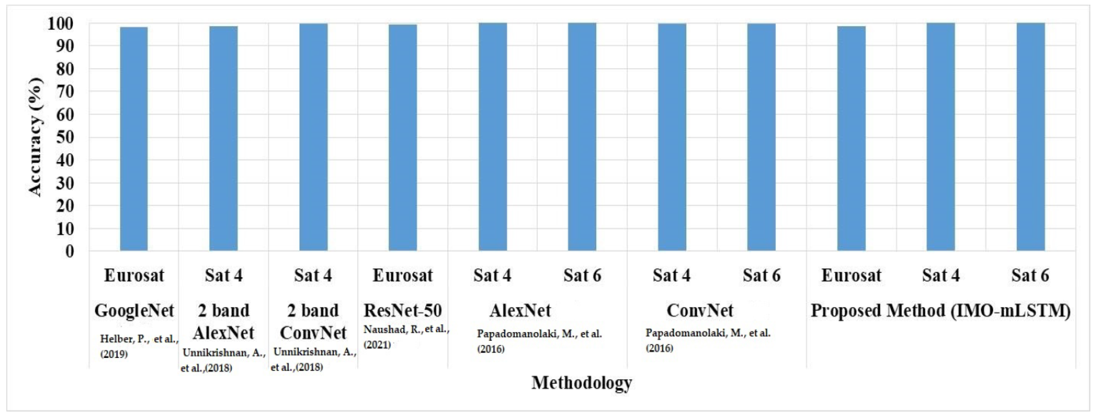
The structure of this research is specified as follows: Section 2 represents the literature review based on satellite image classification. Section 3 explains the proposed method along with the mathematical equations. Section 4 represents the simulation results of the proposed method and its comparative analysis with existing methods. Finally, the conclusion is stated in Section 5.

2. Literature Review

Several techniques have been established by scholars in the field of satellite image classification. Here, detailed surveys about some significant contributions to conventional studies are demonstrated.

An LULC classification with U-Net has been proved by Jonathan V. Solórzano et al. [21] to increase accuracy. The goal was to assess U-nets for Sentinel-1 and 2 images to provide a thorough LULC classification in a tropical region of southern Mexico. Additionally, this assessment compares the outcomes of the U-net and Random Forests (RF) algorithms and evaluates the influence of image input on classification accuracy. Since only spectral characteristics are used in LULC classification, the U-net concludes both spatial and spectral features. Additionally, natural forests and crops have different spatial configurations; the coupling of Synthetic Aperture Radar (SAR) and Multi-Spectral (MS) including U-net aids in the distinction between the pair.

The Eurosat Dataset with Deep Learning Benchmark for LULC classification was given by Helber et al. [22]. The proposed deep Convolution Neural Networks (CNN) offer values for this innovative database with the spectrum portions. Total classification performance was improved using the proposed approach dataset. The classification scheme offers the door to a variety of Earth observation technologies. Furthermore, deep CNN has been used to identify patterns in LULC, as well as improve the geometrical parameters. The map failed to include a large portion of the office buildings that were affected by environmental issues.

Deep AlexNet with minimal amount of trainable variables for satellite image classification has been proven by Unnikrishnan et al. [23]. The accuracy of spatial and spectral data was examined using deep learning algorithms in conjunction with CNN. The AlexNet design was developed with two-band data and a limited portion of filters, and high-level characteristics from the tested model were able to categorize distinct LC classes in the database. In remote sensing studies, the proposed structure with fewer training data reduced the current four-band CNN to frequency groups and decreases the number of filters. Large receptive fields present in the network make it difficult to scan for all characteristics, resulting in low performances.

To improve classification accuracy, Deep Transfer Learning for LULC classification has been demonstrated in [24]. In this study, transfer learning methods such as Visual Geometry Group (VGG16) and Wide Residual Networks (WRNs) were used for LULC classification, utilizing red–green–blue form of the Eurosat data. Additionally, data augmentation has been exploited to assess and validate the efficiency and computational complexity. The limited-data problem was overcome through the recommended manner, and maximum accuracy was accomplished. In spite of utilizing similar data augmentation methods, it exposed that the Wide ResNet-50 generated improved outcomes when compared with VGG16. The class predictability was the only variation observed in the accuracy, apart from that, Wide ResNet-50 provided maximum scores, and its learning patterns were equivalent.

Jayanthi and Vennila [25] presented an adaptable supervised multi-resolution technique for satellite image categorization using the Landsat dataset. The mechanisms of satellite image processing are developed to identify the various objects in satellite images. The suggested versatile supervision is a multi-resolution selection that improves precision and accuracy by using a technique of exploitation and trial samples. Here, large amounts of satellite data accurately transferred quickly but still pose a significant difficulty in this procedure because of moving components, and no sensor has combined the best spectral, geographical, and temporal resolutions.

LC Dataset with CNN for satellite image classification was provided by Emparanza et al. [26] to improve precision, accuracy, and recall. The suggested model was created by an aggregation of two CNN classifiers that specialize in recognizing water areas. This new methodology has shown to be substantially faster and more effective across the board. However, in order to achieve higher accuracy for land cover classification, CNN needs large amounts of training samples, highly dependent land cover features, prediction quality, and dataset reliability. Due to those factors, certain small classification errors have been identified.

For satellite image categorization, Zhang et al. [27] introduced the CNN-Capsule Network (CapsNet) with the UC Merced and AID dataset. The innovative CapsNet design employs the capsule to substitute the neuron in the standard network that was suggested to maintain the geospatial data from the CNN. In addition, the capsule is a vector that may be used to understand part–whole relationships within an image by representing internal attributes. While using the fully connected layer after the classification algorithm reduces the two-dimensional extracted features into a one-dimensional feature map, it takes considerably too long to identify the subclasses.

Multi-spectral satellite data on land cover categorization based on deep learning approaches have been proven by He and Wang [28]. A spectral–texture categorization classifier was developed utilizing wavelet transform’s exceptional texture collection capabilities to acquire relevant details to enhance the spectral feature set, paired with deep learning for feature extraction and selection. For the assessment, multi-spectral imaging satellite data and field measured data were employed. Research findings demonstrate that the suggested approach outperforms exploratory factor analysis, regression methods, and neural networks in terms of improving multi-spectral picture classification accuracy. According to the findings, the various formations of the classed regions generated using the suggested arrangement are well-formed. However, this approach falls short in characterizing how changes in land cover relate to a rise or fall in ecosystem function. Furthermore, the evaluation index fails to capture the scope and rate of change effectively.

From the overall literature works, still, there is a significant need for information about the environment and natural resources; many maps and digital databases that are already in existence were not especially created to fulfil the needs of different users. The kind of classification or legend employed to explain fundamental facts such as land cover and land use is one of the primary causes, while being typically underappreciated. Many of the current classifications are either focused on a single project or use a sectoral approach, and they are generally not comparable with one another. Although there are numerous categorization systems in use around the globe, no single one is universally recognized as the best way to categorize land use or cover. In order to overcome this, this research created a new land cover classification system name called IMO-mLSTM. The suggested methodology is extensive in that it can easily handle any identifiable land cover found anywhere in the world and is applicable at any size. Additionally, the system can be used to evaluate the coherence of current categories, which is clearly described in the following sections.

3. Proposed Method

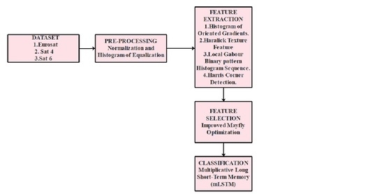
In this research, the elements or features that are found on the Earth’s surface are referred to as land usage and land cover. The Sat 4, Sat 6, and Eurosat are used in this work for experimental research. After gathering the satellite images, pre-processing is conducted using normalization and histogram equalization, which are used to enhance image quality. After normalizing the collected satellite images, feature extraction is carried out to extract the feature vectors from the images utilizing the HOG, LGBPHS, HCD, and Haralick texture features. Using the Improved Mayfly Optimization (IMO) algorithm, feature selection is carried out after the feature vectors are extracted. After extracting the optimal features, the Multiplicative Long Short-Term Memory (mLSTM) network is exploited for classifying the LULC classes. The general process of the satellite image classification is depicted in Figure 1.

3.1. Image Collection

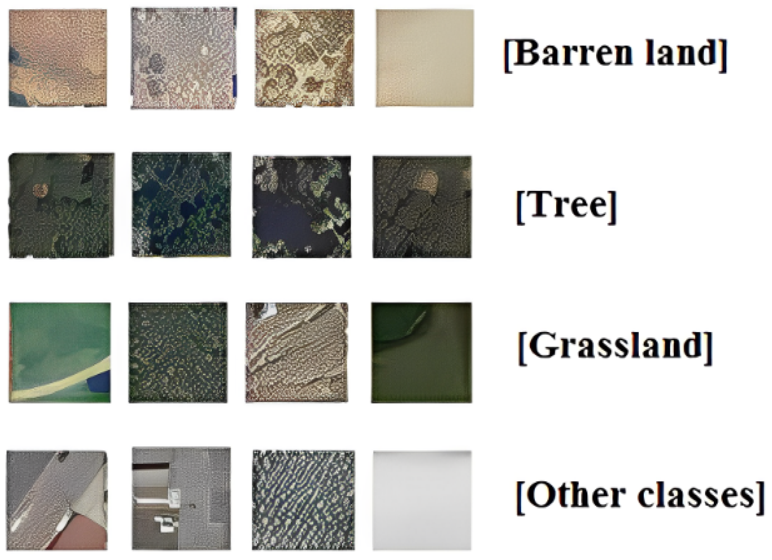
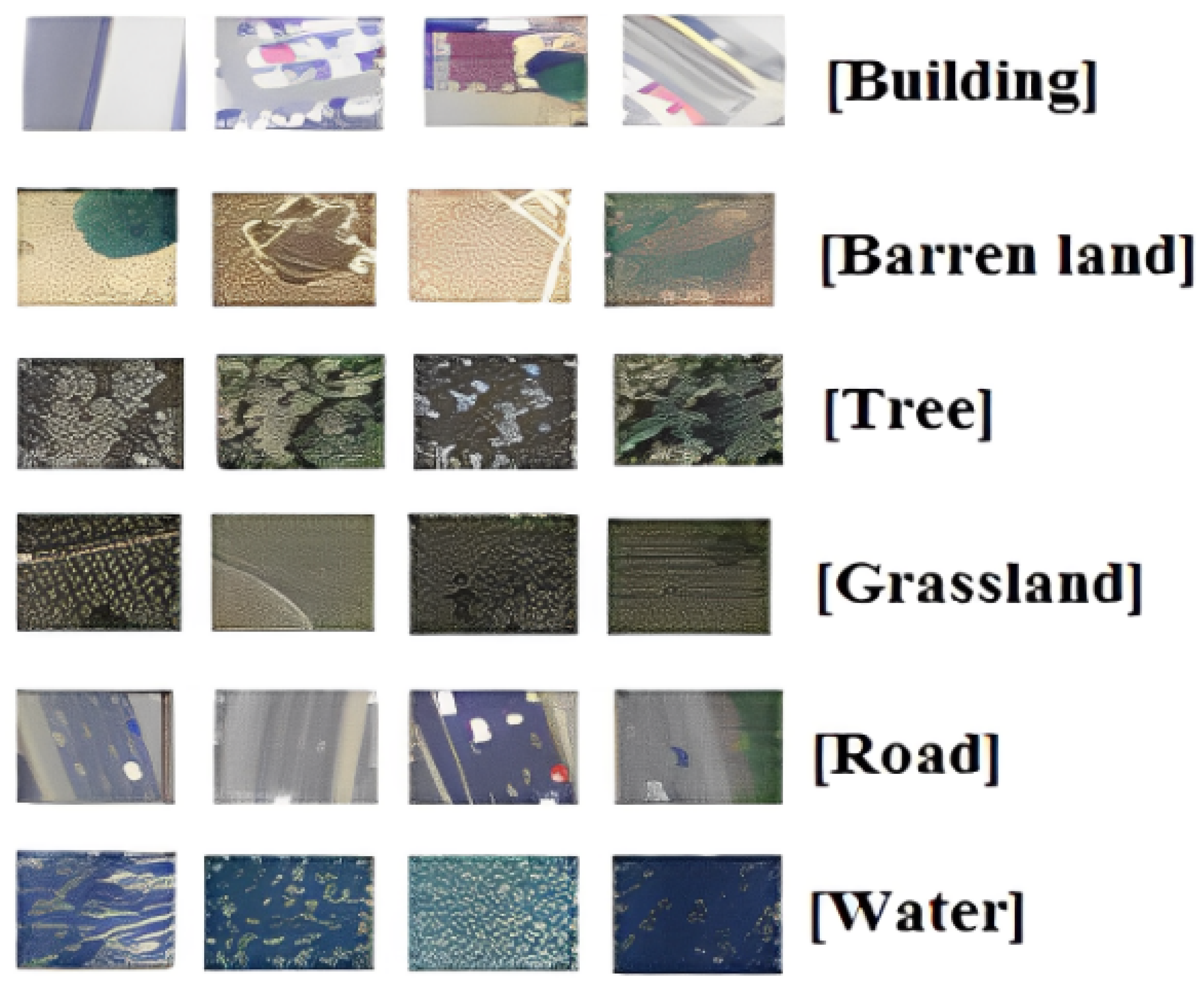
The statistical investigation is applied using the Sat 4, Sat 6, and Eurosat databases to distinguish objects in farming environments. Sat 4 contains 500,000 remote sensing data divided into four categories. Every spatial data image is divided into six LC types. Figure 2 shows an example image from Sat 4 and Sat 6 [23,29].

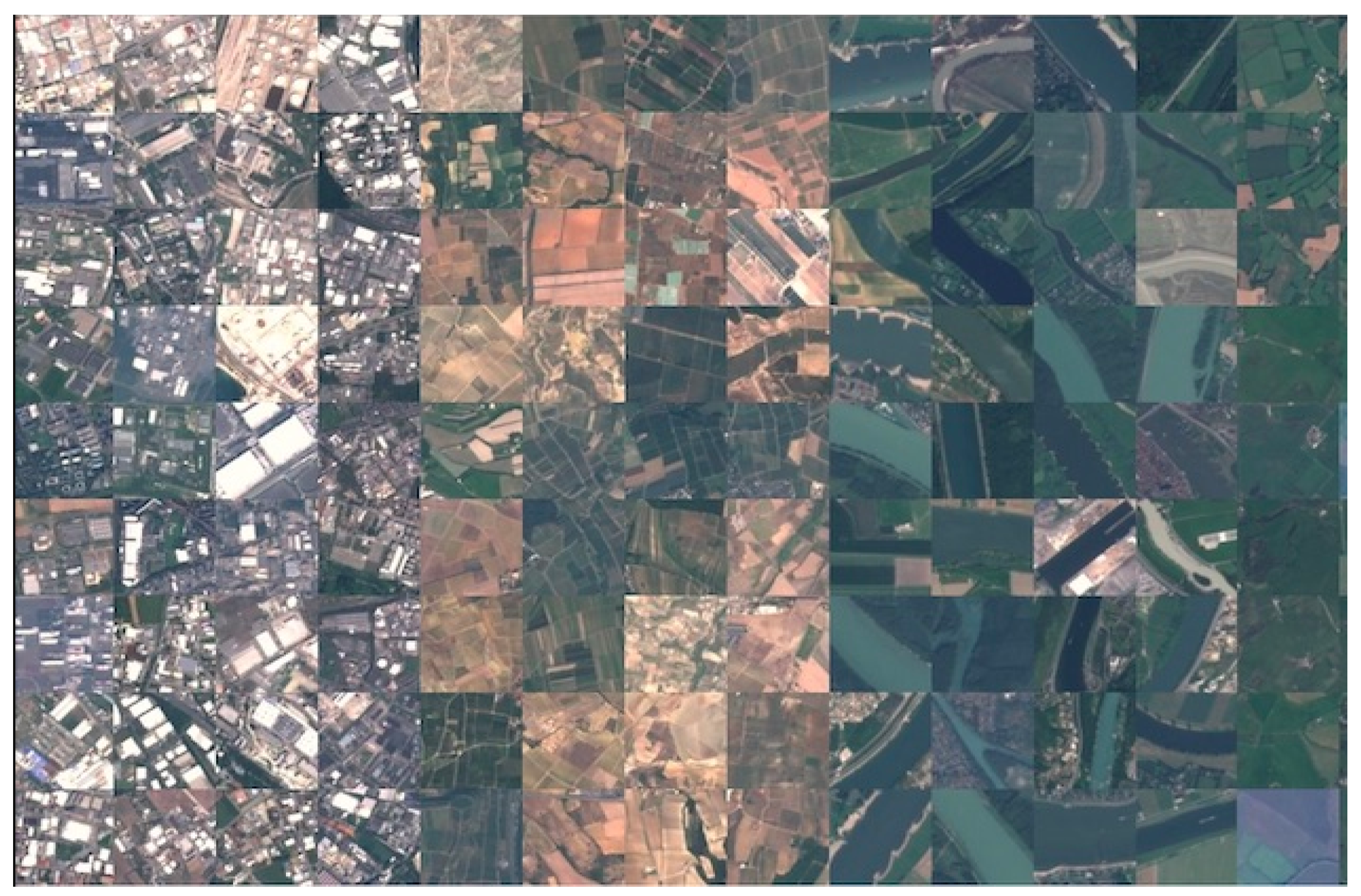
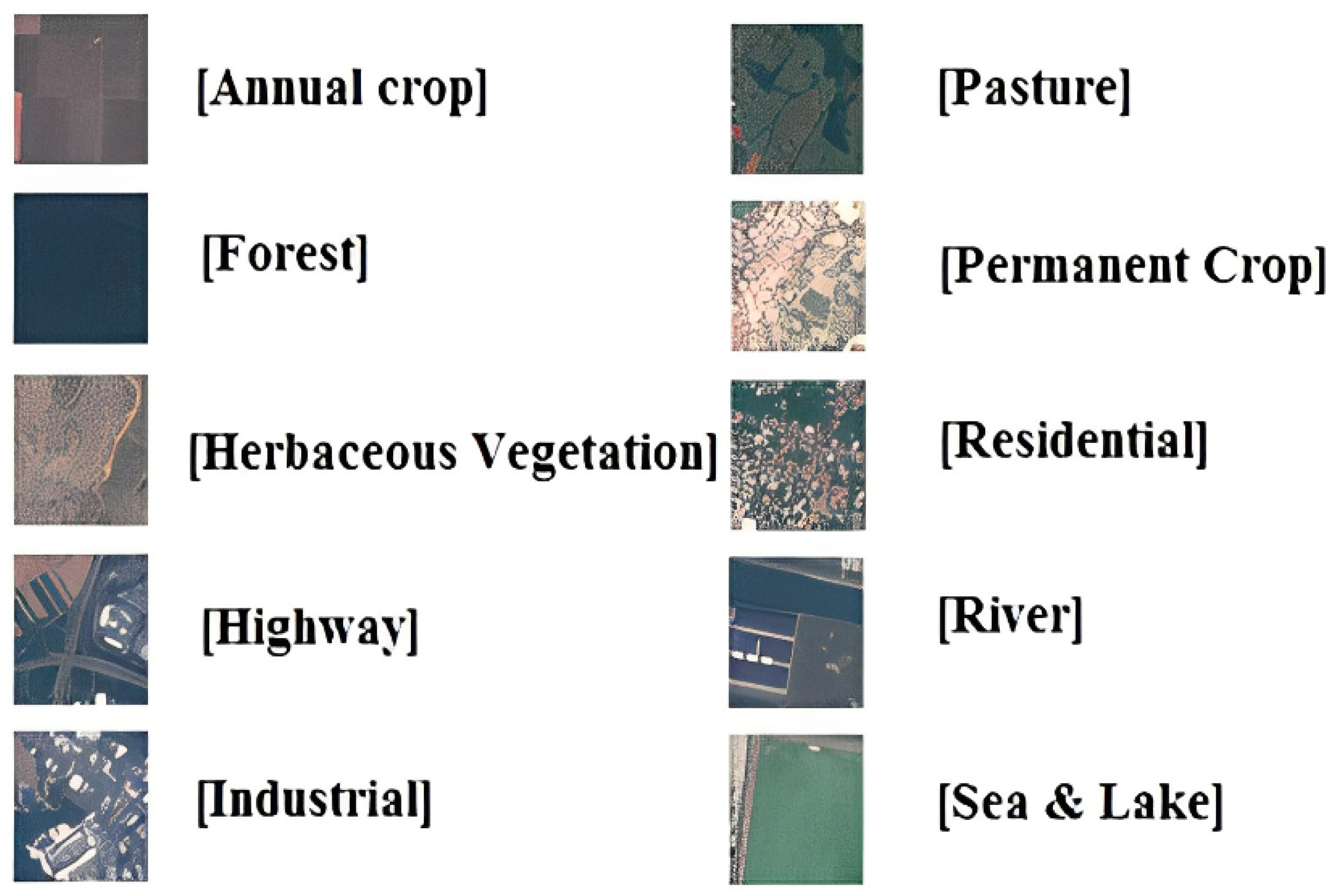
The satellite data were acquired in European cities and scattered across thirty-four nations. Data are obtained with 27,000 annotated and geo-linked texture features, each of which is $64\times 64$ images in size. The Eurosat database is divided into ten classes, each of which comprises 2000–3000 images. Commercial establishments, motorways, and residential complexes are LULC-type data. Figure 3 displays a sample image of the Eurosat database [22,30].

3.2. Image Pre-Processing

To increase the image quality, min–max [31] and z-score normalization procedures are used once the satellite data are collected. Equations (1) and (2) offer general formulas for normalization procedures.

$$I\_out=\left(I\_in-Min\right)\frac{newMax-newMin}{Max-Min}+newMin$$

(1)

where, $MinandMax$ are declared as a minimum and maximum intensity standard; the image following the normalization is stated by $I\_out$, $I\_in$ is stated as an actual satellite image, and the maximum and minimum intensity value is represented as $Max-Min$, which ranges from 0 to 255. In z-score normalization, the data are normalized with respect to their mean (${\mu }_{I\_in}$) and standard deviation (${\delta }_{I\_in}$). For z-score, a normal distribution is often assumed. The distribution to the left and right of the origin line has not been equal if the data are unbalanced. Therefore, $I\_out$ is specified in Equation (2),

$$I\_out=\frac{I\_in-{\mu }_{I\_in}}{{\delta }_{I\_in}}$$

(2)

This normalizing method relies on a mean and standard deviation of the data that might change over time. These normalization methods are helpful for maintaining the linkages between the original input data. Normalization is the finest method for image enhancement since it improves image quality without losing image information [32].

3.3. Feature Extraction

The excellent discriminative strength and partial invariance to color and grayscale images are two significant advantages of feature extraction methods. After normalizing the acquired satellite images, the next are utilized to extract features from the images: Histogram of Oriented Gradients (HOG), LGBPHS, and Haralick texture features such as brightness, coherence, frequency, homogeneous, variance, angular second-moment feature, and Harris Corner Detection (HCD). Since satellite images often cover a significantly bigger area, they have more extensive scientific uses. Airborne images are more suitable for smaller-scale applications such as advertising and marketing since they are captured from a lower height and therefore cover a smaller region. The high-resolution spatial data are collected from airborne imaging, which is frequently employed in this research. Almost any area of the Earth’s surfaces may be imaged in great detail at any time using airborne platforms, which also make it easier to gather data. These airborne images are converted into gray scale for further processing.

HOG: The HOG feature descriptor effectively captures the gradient and edge structure of the objects in satellite images. However, the HOG feature descriptor operates on localized cells, maintaining object orientation as an exception to photometric and geometric invariance. This action aids in identifying changes that appear in vast spatial regions. This classifier effectively preserves the gradient in satellite images, in which the vectors are not aligned properly. This process aids in the detection of changes in wide spatial areas. HOG is usually focused on the gradient direction that builds up over images of a small spatial region, such as a cell. The local 1-D histogram is collected by the HOG descriptor in each cell. The previous procedure involved gathering the local histogram over a large geographic area, usually a block of cells, then using the information to normalize every cell in the block. In this instance, the detection window is positioned high above the grid.

LGBPHS: Using various orientation and scale Gabor filters, the pre-processed satellite images are first modified to create numerous Gabor Magnitude Pictures (GMPs). Each GMP is then transformed into a Local GMP (LGMP), which is further divided into rectangular areas with distinct histograms and sizes. Thus, to create final histogram sequences, the LGMPs of every LGMO map are summarized. Every Local Gabor Binary Pattern (LGBP) map is then further divided into non-overlapping rectangle areas to precise specifications, and histograms are calculated for every region. Finally, the LGBP histograms of every LGBP map are aggregated to produce the image.

Haralick Texture: In terms of contrast, energy, entropy, homogeneity, correlation, and angular second moment, the Haralick features are 2nd order statistics, which depict the overall average degree of correlation between the pixels. This illustrates several measurable textural properties generated from GLCM, a well-liked and widely used statistical measure of textures based on the spatial interdependence of gray images. It frequently results in precise extraction that is resilient in different rotations. The spatial gray-level distribution is represented in two dimensions by the GLCM. The gray-level histogram is used to obtain the features after creating the co-occurrence matrices. The resulting feature vector is created by the calculated features.

Harris Corner Detection (HCD): These HCD features are exploited to divide the background and foreground data. With each configuration, moving the window along a corner point would result in a noticeable change in luminance. In the front of the fingerprints, Harris’ point is significantly more intense than it is in the background. This HCD uses the gray disparity of images to extract corner points as a modification or expansion of the Moravec corner detection. A grayscale image $I$ and window $w\left(x,y\right)$ are assumed to be deliberated through movements of $u$ in $x$-direction and $v$ in $y$-direction.

3.4. Feature Selection

This procedure is deliberated to be an issue of global combinatorial optimization that tries to remove unnecessary, noisy, and redundant data and number of features and produce standard classification accuracy. Once the feature extraction is complete, the process of feature selection is deliberated using the IMO algorithm. Traditionally, the brute-force algorithm attempts to provide systematic relation among presented candidates, and outlier data instances have less relation with other features, but the problem concerned in this technique was higher computational time during the large datasets. During Sequential Forward Selection (SFS), features are consecutively included to a vacant candidate set till the features do not reduce the standard. Contextual Bandit with Adaptive Feature Extraction is a cluster-based model that is usually applied for unlabeled data or unsupervised classification. In supervised learning, applying Contextual Bandit with Adaptive Feature Extraction tends to result in the loss of information in network learning. This research is supervised classification or based on labeled data, so the Contextual Bandit with Adaptive Feature Extraction of cluster technique is not required for this model. These existing feature selection methods do not adaptively select features and tend to select many irrelevant features for classification. So, an optimization algorithm called Improved Mayfly Optimization is introduced in this research that learns the features adaptively and selects the relevant features. Similarly, IMO is less complex compared with the SFS, brute-force algorithm, and Bandit with Adaptive Feature Extraction. All potential combinations of attributes selected from the dataset make up the discrete search space. Considering the low number of features, it could be probable to arrange all the possible feature subsets. In order to determine its own behavior, the improved mayfly uses more group information that confirms the group diversity, thus progressing the stability among exploration and exploitation to improve efficiency.

3.4.1. Mayfly Optimization Algorithm

For the MO approach, mayflies should be separated into male and female entities. Additionally, because male mayflies are always strong, they will perform better in augmentation. The MO uses equivalent parameters as PSO, adjusting their positions depending on the current position $p_i\left(t\right)$ and velocity $v_i\left(t\right)$ at the current iteration count. To update their positions, all males and females apply Equation (3). As an alternative, their velocity is updated in different manners.

$$p_i\left(t+1\right)=p_i\left(t\right)+v_i\left(t+1\right)$$

(3)

The velocity is modified based on current fitness $f\left(x_i\right),$ and best fitness in previous actions is stated as $f\left(x_{h_i}\right)$.

$IF f\left(x_i\right)>f\left(x_{h_i}\right)$, the male mayflies update their current velocities, and their preceding actions are stated in below Equation (4):

$$v_i\left(t+1\right)=g.v_i\left(t\right)+{\alpha }_1{e}^{-\beta {\gamma }_p^2}\left[x_{h_i}-x_i\left(t\right)\right]+{\alpha }_2{e}^{-\beta {\gamma }_g^2}\left[x_g-x_i\left(t\right)\right]$$

(4)

where $g$ is stated as a variable count. ${\alpha }_1,{\alpha }_2, \mathrm{and} \beta$ are exploited as constants. The Cartesian spacing is defined as ${\gamma }_p \mathrm{and} {\gamma }_g$. The array’s distance is the Cartesian distance that is represented below in Equation (5):

$$||x_i-x_j||=\sqrt{{\displaystyle \sum }_{k=1}^n{\left(x_{ik}-x_{jk}\right)}^2}$$

(5)

Alternatively,$IF f\left(x_i\right)<f\left(x_{h_i}\right)$, the male mayflies could modernize their quickness from the current location through a dance coefficient $d$, which is represented in Equation (6).

$$v_i\left(t+1\right)=g.v_i\left(t\right)+d.{\gamma }_1$$

(6)

where ${\gamma }_1$ and ${\gamma }_2$ represent the indiscriminate amount in the distribution and are identified within a range [–1, 1]. As an outcome in the $i^{th}$ female mayfly,$IF f\left(y_i\right)<f\left(x_i\right)$, Equation (7) is stated as:

$$v_i\left(t+1\right)=g.v_i\left(t\right)+{\alpha }_3{e}^{-\beta {\gamma }_{mf}^2}\left[x_i\left(t\right)-y_i\left(t\right)\right]$$

(7)

where ${\alpha }_3$ is referred to as an alternative constant that is applied to stabilize the rapidity. Cartesian distance in the middle of them is represented as ${\gamma }_m$. $IF \left(y_i\right)<f\left(x_i\right)$, the female mayflies adjust their velocities until the previous runout in the course of supplementary dance coefficients $fl$, which are expressed as Equation (8).

$$v_i\left(t\right)=g.v_i\left(t\right)+fl.{\gamma }_2$$

(8)

Their kids progress arbitrarily from their moms, as seen in Equations (9) and (10), respectively.

$$offspring1=L\times male+\left(1-L\right)\times female$$

(9)

$$offspring1=L\times female+\left(1-L\right)\times male$$

(10)

$L$ is declared as subjective data in Gauss distribution.

3.4.2. Improved MO Algorithm

According to the previous equations, Candidates vary their velocities randomly in particular environments. In complex circumstances, efficient systems might be used to adjust the velocities. The global best candidate is chosen by comparing the present velocities and additional weighted distance to modify specific velocities. In addition, Equation (11) determines whether the balanced distance’s halves appear as follows:

$$v_p={\alpha }_i{e}^{-\beta {\gamma }_j^2}\left(p_j-p_i\right)$$

(11)

If the distance between the $j^{th}$ and $i^{th}$ individuals is prolonged, it seems that ${\gamma }_j$ is superior. Consequently, if $p_j$ is distant from $p_i$, it updates its velocity with a lesser magnitude, while $p_j$ is near to $p_i$, it updates with a large magnitude. Thus, Equation (11) should be changed according to the circumstance, as indicated in Equation (12):

$$v_p={\alpha }_i{e}^{-\frac{\beta }{{\gamma }_j}}\left(p_j-p_i\right)$$

(12)

Table 1. Selected feature vectors.

Datasets	Extracted Features	MO Selected Features	IMO Selected Features
Eurosat	$9000\times 55$	$9000\times 49$	$9000\times 43$
Sat 4	$5000\times 38$	$5000\times 32$	$5000\times 27$
Sat 6	$8700\times 50$	$8700\times 46$	$8700\times 40$

shows the extracted and selected feature vectors after exploiting the IMO method. While referring to Table 1, from the available datasets, the outcomes (features) are extracted. Those features are extracted based on a filtered process which depends on the dataset’s general properties (some measure such as correlation), such as correlation with the multi-variate regression. IMO-based feature selection techniques remove the redundant and noisy data to choose a subset of appropriate features by means of Improved Mayfly Optimization algorithms to improve classification outcomes, which are usually quicker, more effective, and minimize overfitting.

By analyzing Table 1, it clearly shows that the proposed IMO-based feature selection reduces the number of extracted features from the collected dataset (Eurosat, Sat 4 and Sat 6) when compared with MO-based feature selection. Table 1 denotes that the proposed IMO selected 9000 images with 43 lengths of features in the Eurosat dataset; wherein the Sat 4 dataset, 5000 images with 27 lengths of features were selected, and in the Sat 6 dataset, 8700 images with 40 lengths of features were selected.

3.5. Classification

LSTM is a type of deep learning model for image classification which has been shown to achieve the highest level of accuracy [33]. An LSTM network can be used to train a deep neural network to categorize system data. In LSTM, IMO-selected features are used as inputs, and the number of classes is considered as output. LSTMs perform considerably better since they are skilled at remembering particular patterns. As they pass through each layer, the relevant data are saved and the irrelevant data are eliminated in each and every cell. The default behavior of the multiplicative LSTM classifier is to recollect relevant data for an extended period. To achieve a better result in LULC classification, more remote sensing data must be processed. The mLSTM classifier is the preferred place for LULC classification when this factor is taken into account. The mLSTM classifier, in particular, is made up of a succession of mLSTM units that contain quasi-periodic information for extracting long- and short-term relationships. The supervised classification approach exploited in this research is the mLSTM classifier. The theory behind supervised classification is that a user can select testing image values that are reflective of some classes present in these images and can then inform the data visualization tools to use certain training data as references for categorizing all other images. Multiplicative LSTM models appear to gain embedding matching for secondary operational motifs to improve the quality.

3.5.1. Process of LSTM

The data flow in and out of the internal positions of system is managed by a sequence of multiplicative gates in the widely used RNN design, which is known as LSTM. There are a number of marginally distinct LSTM variants employed in the trials. The hidden state obtains the inputs from the input layer, which is stated as $x_t$, and its previous hidden state is represented as $h_{t-1}$, which is formulated in Equation (13)

$${\widehat{h}}_t=W_{hx}{x}_t+W_{hh}{h}_{t-1}$$

(13)

The LSTM consists of 3 gating units—one is input gate $i$, second is output gate $o$, and third is forget gate $f$ for recurrent and feed-forward networks, which are expressed in Equations (14)–(16):

$$i_t=\sigma \left(W_{ix}{x}_t-W_{ih}{h}_{t-1}\right)$$

(14)

$$o_t=\sigma \left(W_{ox}{x}_t-W_{oh}{h}_{t-1}\right)$$

(15)

$$f_t=\sigma \left(W_{fx}{x}_t-W_{fh}{h}_{t-1}\right)$$

(16)

Here, the logistic sigmoid function is stated as $\sigma$. $f$ decides the quantity of prior internal state $c_{t-1}$ that is kept, while $i$ manages the quantity of input to every hidden unit to internal state vector $c_t$. With the help of $f$, the network is able to decide if the data ought to be stored and rewritten during every time interval. Updating the internal state is performed through Equation (17),

$$c_t=f_t \odot c_{t-1}+i_t \odot \tanh \left({\widehat{h}}_t\right)$$

(17)

The amount of every unit’s activation is conserved and determined by the output gate. It enables the LSTM cell to store data that may become important in the future but is not necessary for the current output. The concealed state’s final output is represented by Equation (18).

$$h_t=\tanh \left(c_t\right) \odot o_t$$

(18)

The capacity of the LSTM to regulate how data are stored in every unit was generally effective.

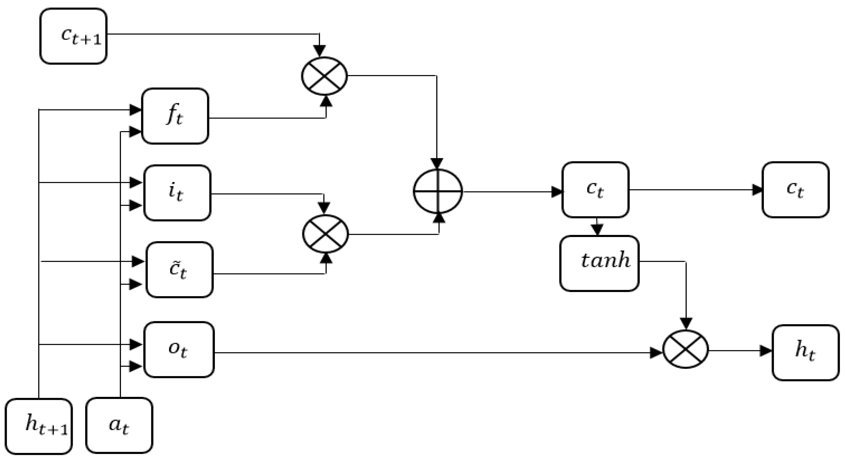
3.5.2. Multiplicative LSTM

Like any other NN, mLSTM has the potential to have several hidden layers. The following hyper-parameters are used in MLSTM. They are, initial learning rate (0.001), Neurons (100), Layers (10), and Epoch (100) with Adam optimizer. The mLSTM, a hybrid design which integrates the hidden-to-hidden transition of RNNs by the LSTM gating framework, is suggested for controlling the over-fitting problem. By connecting each gating unit in the LSTM to the intermediate state $m_t$ of the RNN, the conventional RNN and LSTM designs can be merged to create the following Equations (19)–(23).

$$m_t=\left(W_{mx}{x}_t\right) \odot \left(W_{mh}{h}_{t-1}\right)$$

(19)

$${\widehat{h}}_t=W_{hx}{x}_t+W_{hm}{m}_t$$

(20)

$$i_t=\sigma \left(W_{ix}{x}_t-W_{im}{m}_t\right)$$

(21)

$$o_t=\sigma \left(W_{ox}{x}_t-W_{om}{m}_t\right)$$

(22)

$$f_t=\sigma \left(W_{fx}{x}_t-W_{fm}{m}_t\right)$$

(23)

Set $m_t$ and $h_t$ dimensions to be the same for all the trials. A network with 1.25 times as many recurrent weights as LSTM for identical hidden layers is produced by choosing to share $m_t$ over every LSTM unit category. This architecture aims to combine the extended time lag and overall functioning of LSTMs with the adaptable input-dependent transitions of RNNs. It might be simpler to control the transitions that arise from the factorized hidden weight matrix. More adaptable input-dependent transition patterns than conventional LSTM and RNNs are made possible by the supplementary sigmoid input and $f$, which are present in multiplicative LSTM. Figure 4 shows the graphical depiction of multiplicative LSTM.

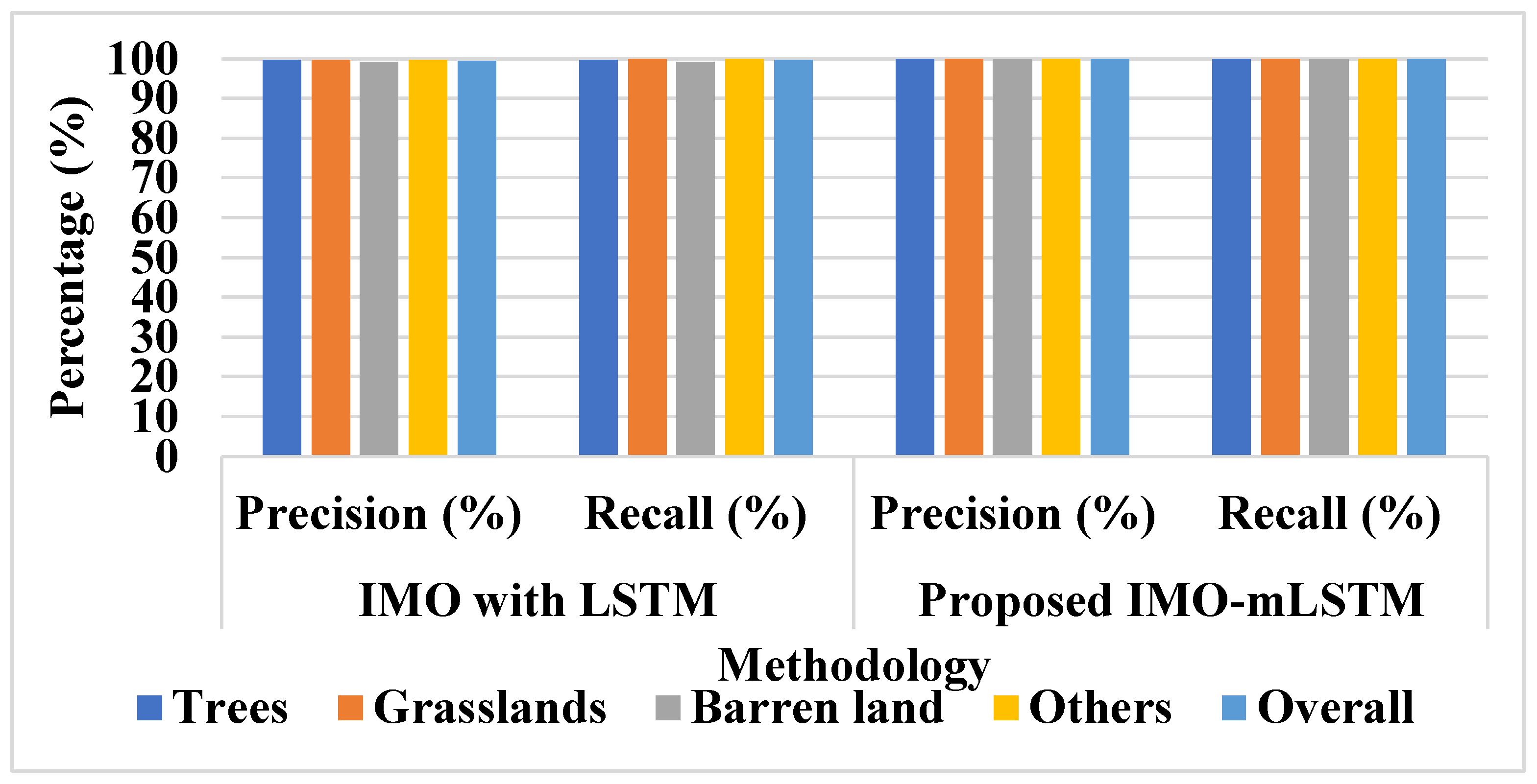
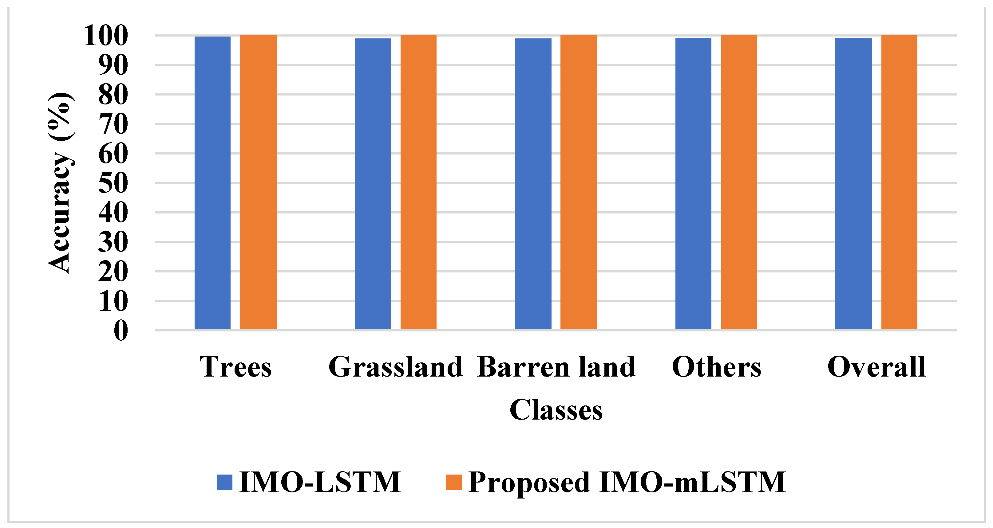
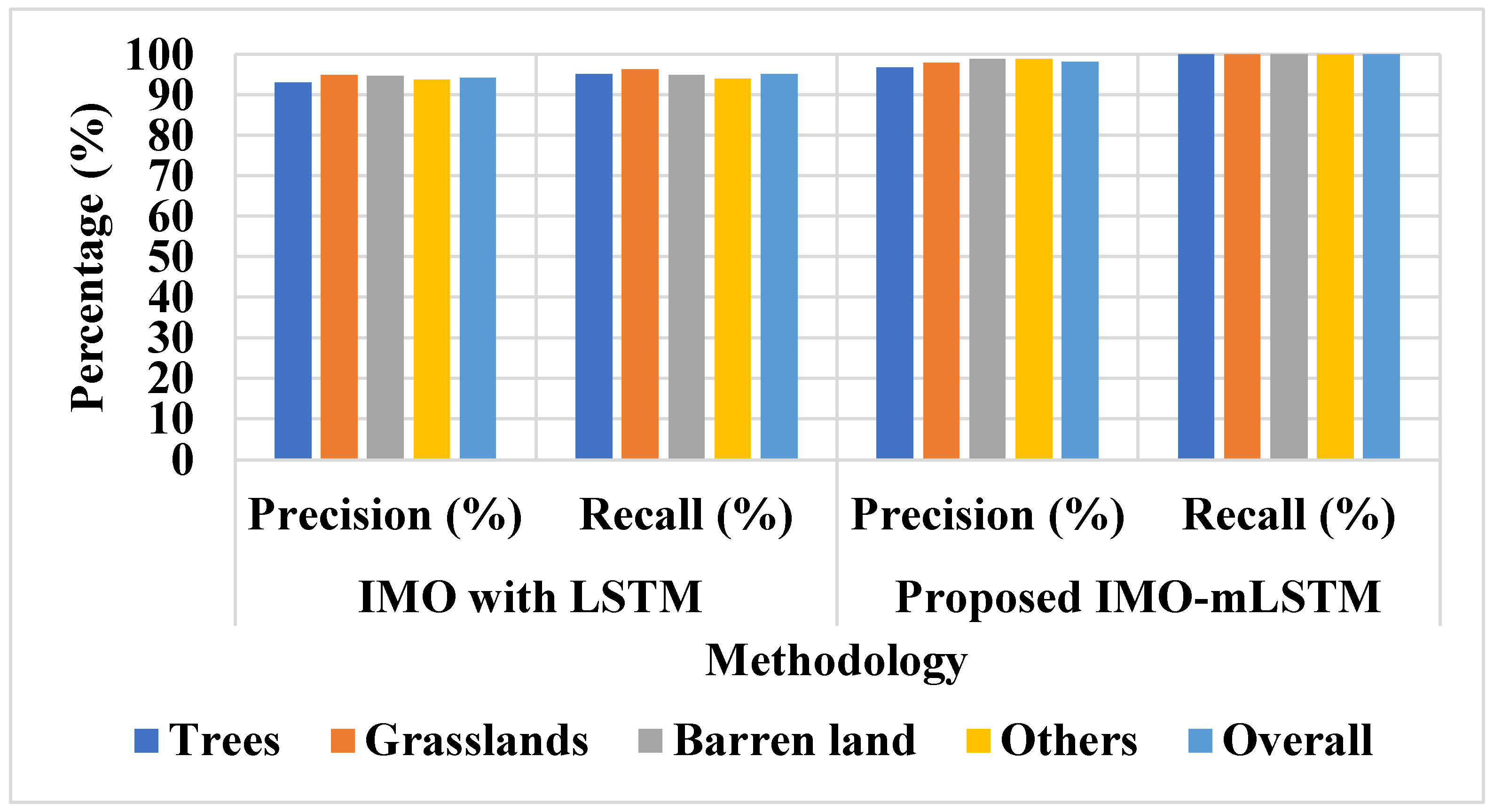
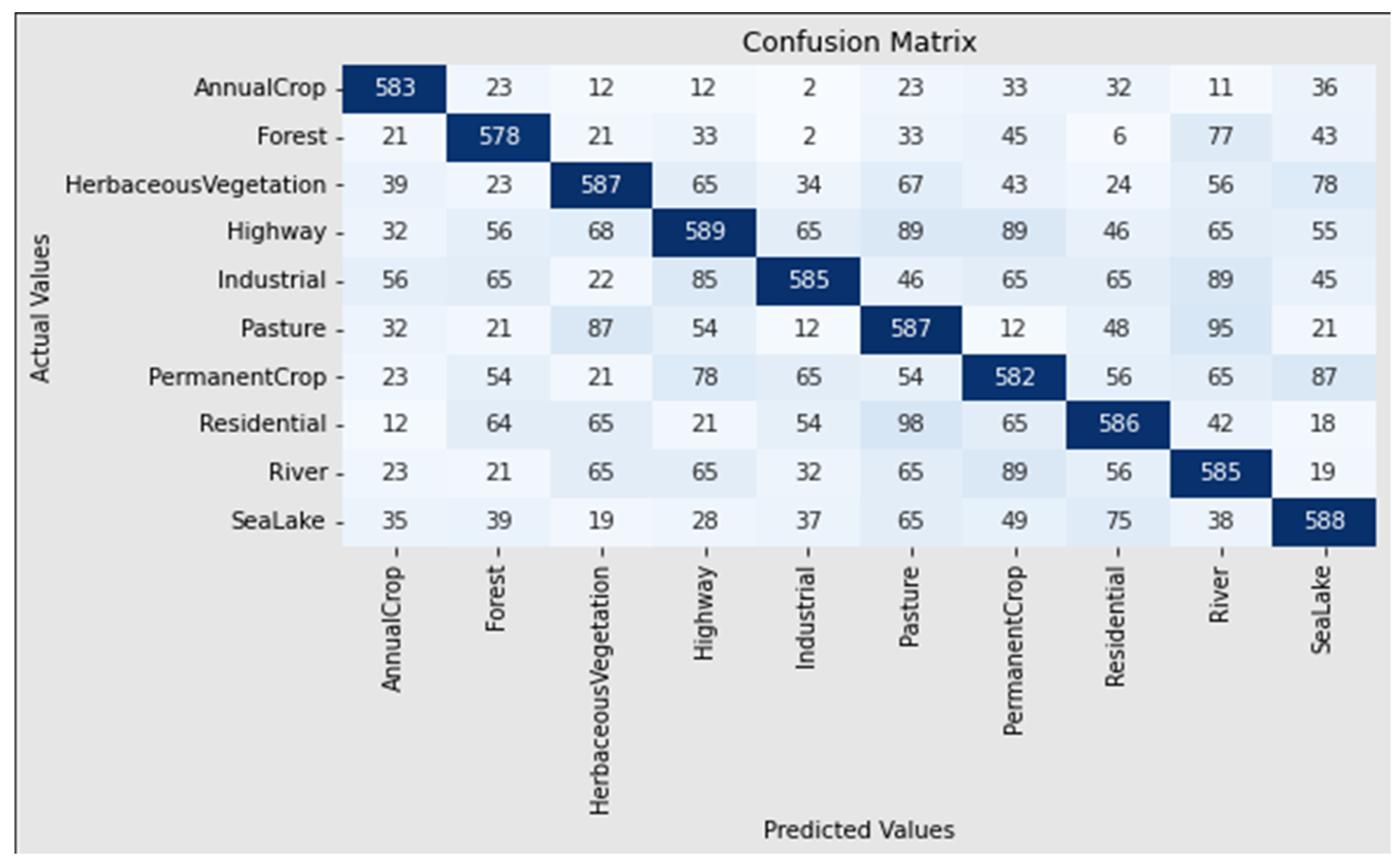
Landscape metrics for LULC classification are a less-explored aspect of spatial analysis and image classification. This study demonstrates how several shape- and size-associated landscape measurements may be used as input layers in the categorization process. Precision, recall, and accuracy are used to assess the suggested model’s performance in this study. Equations (24)–(26) represent the mathematical formulations of accuracy, recall, and precision.

$$Accuracy=\frac{TP+TN}{FN+TP+TN+FP}\times 100\%$$

(24)

$$Recall=\frac{TP}{TP+FN}\times 100\%$$

(25)

$$Precision=\frac{TP}{TP+FP}\times 100\%$$

(26)

where $TN$ is stated as true negative, $FN$ is specified as false negative, $TP$ is signified as true positive, and $FP$ is signified as a false positive.

4. Results and Discussion

In this study, a MATLAB 2020a setting containing 128 GB RAM, i9 Intel core processor, Windows 10 operating system (64 bit), 2080Ti Graphic Processing Unit (GPU) 22 GB, and 3 TB hard disk is exploited for simulation modeling. The suggested model’s effectiveness is performed in the presence of a few standard models in this research. This system is a thorough, standardized a priori classification system created to satisfy certain user needs and guarantee a high degree of geographic accuracy. The classification uses a collection of independent diagnostic criteria that are clearly stated, referred to as classifiers, to enable correlation with pre-existing classifications and legends. As a result, this approach might be used as a base to reference land cover.

4.1. Performance on Sat 4 Dataset

This dataset is exploited to assess the projected method’s effectiveness in categorizing four LC classes. With 70% training and 30% testing of the data, the overall performance is confirmed for 500,000 satellite data. The proposed method with different classifiers: IMO with LSTM was evaluated in

Table 2. Performance analysis on Sat 4.

Classes	IMO with LSTM		Proposed IMO-mLSTM
	Precision (%)	Recall (%)	Precision (%)	Recall (%)
Trees	99.54	99.65	99.99	99.98
Grasslands	99.6	99.87	99.98	99.97
Barren land	99.07	99.12	99.92	99.99
Others	99.61	99.9	99.99	99.98
Overall	99.45	99.635	99.97	99.98

and

Table 3. Performance analysis of accuracy on Sat 4.

Classes	Accuracy
	IMO with LSTM	Proposed IMO-mLSTM
Trees	99.57	99.99
Grasslands	98.8	99.98
Barren land	98.9	99.992
Others	99.15	99.993
Overall	99.1	99. 94

. Table 2 and Table 3 clearly show that the proposed IMO-mLSTM classifier increases LULC classification accuracy by up to 1% when related to conventional classifiers. Figure 5 displays the behavior of precision and recall on the Sat 4 dataset. Figure 6 illustrates the behavior of accuracy on the Sat 4 dataset.

Table 4. Performance analysis of recall and precision on the Sat 4 dataset.

Classes	IMO with LSTM		Proposed IMO with mLSTM
	Precision (%)	Recall (%)	Precision (%)	Recall (%)
Trees	93	95	96.61	99.98
Grasslands	94.9	96.1	97.92	99.96
Barren land	94.65	94.92	98.79	99.99
Others	93.7	94	98.69	99.98
Overall	94.06	95.005	97.99	99.98

and

Table 5. Performance analysis of classification accuracy on the Sat 4 dataset.

Classification Accuracy (%)
Classes	LSTM	IMO with LSTM	Proposed IMO with mLSTM
Trees	93	97.84	99.99
Grasslands	94.44	95.89	99.98
Barren land	94.5	96.92	99.992
Others	93.92	97.78	99.993
Overall	93.965	97.1	99.984

show the effectiveness of the proposed scheme using other optimizers such as IMO. According to Table 4 and Table 5, the suggested mLSTM classifier with IMO performed better in LULC categorization. In comparison with IMO-LSTM, the suggested model (IMO with mLSTM) demonstrated a maximum of 6.017% and a minimum of 1.652% increase in LULC. Figure 7 presents the behavior of precision and recall on Sat 4. Figure 8 presents the behavior of accuracy on various classes with several algorithms, while Figure 9 shows the visual results of the Sat 4 dataset. Figure 10 shows the confusion matrix for the Sat 4 dataset.

4.2. Performance Analysis on the Sat 6 Dataset

The Sat 6 dataset is used to evaluate the developed efficacy while classifying six different types of LCs: grassland, water bodies, buildings, barren ground, roads, and trees. The effectiveness of 40,500 satellite images is evaluated, with 70% of the data being trained and 30% being tested. The proposed method (mLSTM-IMO) obtained better results when compared with other classification methods such as LSTM and IMO methods in terms of recall, and precision which are shown in

Table 6. Performance analysis of precision and recall on the Sat 6 dataset.

Classes	IMO with LSTM		IMO-mLSTM
	Precision (%)	Recall (%)	Precision (%)	Recall (%)
Barren land	97.012	98.86	99.94	99.99
Trees	98.34	99.1	99.99	99.99
Grasslands	98.65	98.47	99.85	99.93
Roads	98.12	99.23	99.56	100
Buildings	99.5	99.17	99.47	99.99
Water bodies	98.6	98.33	99.99	100
Overall	99.93	98.35	99.96	99.987

. In comparison with other classification strategies, the proposed mLSTM classifier performed better accuracy in LULC classification which is shown in

Table 7. Performance analysis of classification accuracy on the Sat 6 dataset.

Classification Accuracy (%)
Classes	IMO with LSTM	Proposed IMO-mLSTM
Barren land	99.1	99.99
Trees	99.12	99.93
Grasslands	98.15	99.99
Roads	98.44	99.99
Buildings	99.1	99.99
Water bodies	98.99	99.98
Overall	99.06	99.985

. The proposed mLSTM classifier achieved 99.94% precision, 99.97% recall, and 99.97% accuracy in this database. Figure 11 shows the performance analysis of precision and recall on the Sat 6 dataset. Figure 12 shows the classification accuracy on the Sat 6 dataset, while Figure 13 shows the visual results of the Sat 6 dataset. Figure 14 shows the confusion matrix for the Sat 6 dataset.

4.3. Performance Analysis on Eurosat

The proposed methodology for identifying 12 LULC classes in the Eurosat database. The performance of 27,000 satellite data is evaluated in this scenario, with 70% of the data being trained and 30% being tested.

Table 8. Performance analysis of the proposed method on Eurosat.

Average Value
Classification	Optimizers	Precision (%)	Recall (%)	Accuracy (%)
	PSO	87.89	90	88.2
LSTM	HGO	90	92.02	90
	IMO	91.38	92.91	90.09
	PSO	92	93.98	95
mLSTM	HGO	94.5	94	96.9
	IMO	97.9	98.8	97.8

compares the suggested performance of the model to that of existing classifiers and optimizers such as LSTM and Particle Swarm Optimization (PSO), Human Group Optimizer (HGO), and IMO. As a result, the suggested mLSTM classifier with the IMO optimizer has an accuracy, recall, and precision of 97.80%, 98.80%, and 97.90%, respectively. The examination clearly shows that the proposed mLSTM classifier by IMO optimizer displayed enhanced results in LULC classification. Figure 15 shows the performance of precision, recall, and accuracy on Eurosat, while Figure 16 shows the visual results of the Eurosat dataset. Figure 17 shows the confusion matrix for the Eurosat dataset.

4.4. Comparative Analysis

Table 9. Comparative Analysis of Accuracy.

Approach	Dataset	Accuracy (%)
GoogleNet [22]	Eurosat	98.18
2-band AlexNet [23]	Sat 4	98.45
2-band ConvNet [23]	Sat 4	99.66
ResNet-50 [24]	Eurosat	99.17
AlexNet [29]	Sat 4	99.98
	Sat 6	99.93
ConvNet [29]	Sat 4	99.86
	Sat 6	99.90
Proposed Method (IMO-mLSTM)	Eurosat	98.52
	Sat 4	99.99
	Sat 6	99.98

shows the results of the comparison study between the proposed and previous methods. The proposed model includes two bands of information and smaller filters that are evaluated to categorize images into dissimilar categories. The created method was associated with prior networks in light of precision, recall, and accuracy in various literature. In this paper, an enhanced mayfly optimization technique is integrated with the mLSTM classifier to improve the performance of LULC. The suggested feature selection approach enables the mLSTM classifier, which achieves higher performance of the classifier by reducing the “curse of dimensionality”. Figure 18 shows the comparative analysis of accuracy. In Table 9, the proposed IMO-mLSTM is compared with existing classes named GoogleNet [22], 2-band AlexNet [23], 2-band ConvNet [23], ResNet-50 [24], AlexNet [29], and ConvNet [29] in terms of accuracy.

By reaching 99.17% accuracy, the results demonstrate that the ResNet-50 [24] has outclassed the proposed best outcomes in terms of accuracy performance. While the proposed IMO-mLSTM converted RGB into a grayscale image, the existing ResNet-50 [24] used the RGB version of the EuroSAT dataset. As a result, the classification accuracy was lower than the ResNet-50 that was already in place [24]. If the proposed method were to train on RGB data (original data), it would be able to outperform ResNet-50 [24].

According to the reference [28], most land cover categorization methods rely heavily on spectral data while ignoring spatial data. A multi-spectral land cover categorization system is suggested that incorporates air spectrum data and deep learning. A spectral–texture method for conveying the multi-information of features is assembled utilizing second-generation wavelet transform’s excellent depth information to seize the opportunity to secure relevant details to complement the spectral feature space. The results demonstrate that using a Deep Belief Network (DBN) to combine spectral–texture elements of images can increase classification accuracy and extract the spatial patterns law of multi-spectral remote data more effectively.

Table 10. Comparative analysis of accuracy on the Landsat dataset.

Classification Accuracy (%)
Existing DBN [28]	IMO with LSTM	Proposed IMO with mLSTM
81	87	91

shows the comparative analysis of various approaches with Landsat dataset.

From Table 10, it can be clearly inferred that the proposed IMO with mLSTM achieves a better classification accuracy of 91%, which is superior to existing DBN [28] and IMO with LSTM which attain only 81% and 87%, respectively. Figure 19 shows the comparative analysis graph for accuracy performance.

5. Conclusions

This research proposed an effective strategy to classify LULC types using a validated classification procedures name called multiplicative LSTM (mLSTM). The protocol uses picture segmentation and essential data to improve initial reflectance-based categorization and subsequent separation. The findings suggest that accurate classification requires more than just spectral data gathering. The image features were extracted from the normalized satellite data in this research. The improved Mayfly Optimization (IMO) technique was then utilized to select the optimal vectors, which helped to improve the performance of the classifier. An mLSTM classifier was provided with the optimum selected features as input. While related to existing LULC classification techniques, the proposed technique outperformed them on the basis of recall, accuracy, and precision. The simulation results conclusively demonstrate that the suggested IMO-mLSTM approach attained the classification accuracy of 99.99% on Sat 4, 99.98% on Sat 6, and 98.52% on Eurosat datasets. However, the proposed IMO with mLSTM takes a longer time and requires more memory to train the data. Therefore, future research will integrate a hybrid optimization-based strategy in the developed framework for further enhancing LULC classification with less duration.