
Downscaling Satellite-Based Estimates of Ocean Bottom Pressure for Tracking Deep Ocean Mass Transport


1
Joint Institute for Regional Earth System Science and Engineering, University of California-Los Angeles, Los Angeles, CA 90095, USA
2
Jet Propulsion Laboratory, California Institute of Technology, Pasadena, CA 91109, USA
*
Author to whom correspondence should be addressed.
Remote Sens. 2022, 14(7), 1764; https://doi.org/10.3390/rs14071764
Submission received: 22 February 2022
/
Revised: 1 April 2022
/
Accepted: 2 April 2022
/
Published: 6 April 2022
(This article belongs to the Section Ocean Remote Sensing)
Abstract
:Gravimetry measurements from the GRACE and GRACE-Follow-On satellites provide observations of ocean bottom pressure (OBP), which can be differenced between basin boundaries to infer mass transport variability at a given level in the deep ocean. However, GRACE data products are limited in spatial resolution, and conflate signals from many depth levels along steep continental slopes. To improve estimates of OBP variability near steep bathymetry, ocean bottom pressure observations from a JPL GRACE mascon product are downscaled using an objective analysis procedure, with OBP covariance information from an ocean model with horizontal grid spacing of ∼18 km. In addition, a depth-based adjustment was applied to enhance correlations at similar depths. Downscaled GRACE OBP shows realistic representations of sharp OBP gradients across bathymetry contours and strong currents, albeit with biases in the shallow ocean. In validations at intraannual (3–12 month) timescales, correlations of downscaled GRACE data (with depth adjustment) and in situ bottom pressure recorder time series were improved in ∼79% of sites, compared to correlations that did not involve downscaled GRACE. Correlations tend to be higher at sites where the amplitude of the OBP signal is larger, while locations where surface eddy kinetic energy is high (e.g., Gulf Stream extension) are more likely to have no improvement from the downscaling procedure. The downscaling procedure also increases the amplitude (standard deviation) of OBP variability compared to the non-downscaled GRACE at most sites, resulting in standard deviations that are closer to in situ values. A comparison of hydrography-based transport from RAPID with estimates based on downscaled GRACE data suggests substantial improvement from the downscaling at intraannual timescales, though this improvement does not extend to longer interannual timescales. Possible efforts to improve the downscaling technique through process studies and analysis of alongtrack GRACE/GRACE-FO observations are discussed.
1. Introduction
The observation of mass transport integrated across ocean basins is of critical importance for understanding the ocean’s role in climate variability. In particular, the difference between the mass transport in the shallow and deep ocean—the overturning circulation—is the largest contributor to meridional heat transport that moves heat poleward e.g., [1,2]. Integrated mass transports at specific levels of the ocean also determine the movement of water masses, especially in the deep ocean, e.g., [3]. Given its significance, the variability of the overturning circulation has been estimated using numerous in situ measurement campaigns, mostly focusing on the Atlantic Meridional Overturning Circulation (AMOC). The Rapid Climate Change (RAPID) mooring array [4] has tracked the variability of meridional transport in the Atlantic across 26.5N since 2004, and more recently other cross-basin arrays have been deployed at other latitudes in the Atlantic (see [5] for a summary of these efforts). Most of these estimates rely on profiling temperature and salinity (and thus density) at ocean boundaries, in order to compute dynamic height anomalies at the boundaries and hence the (baroclinic) geostrophic transport between them, e.g., [4,6,7,8]. Some of these efforts are also complemented by in situ measurements of the ocean bottom pressure (OBP) at the boundaries, e.g., [7], from which variations of the full geostrophic (barotropic + baroclinic) transport can be inferred. Each of these approaches have their challenges: continuous direct measurement of temperature and salinity at a fixed mooring location is costly, while in situ bottom pressure sensors have limited lifetimes and are subject to spurious exponential and linear drifts. Moreover, the existing time series of integrated cross-basin mass/volume transports are limited mostly to a few latitudes in one ocean basin.
In contrast, the Gravity Recovery and Climate Experiment (GRACE) and GRACE Follow-On (GRACE-FO) satellites, with nearly continuous temporal coverage since 2002, have observed mass change variations of land-based ice and liquid water content, and of pressure variations at the bottom of the ocean, which can then be used to infer geostrophic transport between ocean boundaries. Unlike in situ pressure sensors, GRACE-derived OBP products are not subject to substantial drifts, and the 15-year time span of the original GRACE deployment enables the study of interannual as well as subannual variability. Ref. [9] found that detrended meridional estimates of deep ocean mass transport from GRACE closely agree with in situ estimates from RAPID density-observing moorings on interannual timescales. High correlations between GRACE-derived products and in situ bottom pressure sensors have also been identified at shorter timescales [10,11]. GRACE OBP data can also be synthesized with satellite altimetry and upper ocean hydrographic data (e.g., Argo) to obtain estimates of meridional heat transport and convergence [12] and validate decadal trends in ocean mass and heat content [13].
Even with the extensive spatial and temporal coverage of GRACE, the coarse spatial and temporal resolution of GRACE data products limits their ability to resolve mass/volume transports at specific depth levels. A few studies have used ocean models to assess these limitations and improve GRACE-based estimates of basin-wide transports. Ref. [14] used a pattern-filtering method that mapped the GRACE spherical harmonic solutions, then reconstructed the OBP at a given point using the mapped values weighted based on spatial correlations in an ocean model (FESOM). Refs. [15,16] used fits of GRACE spherical harmonics onto model-derived empirical orthogonal functions to obtain higher-resolution OBP. When validated with in situ bottom pressure data, these approaches indicated some improvement in the OBP estimate relative to the existing GRACE spherical harmonic solutions, e.g., [17]. Compared to spherical harmonic solutions, GRACE mascon solutions have a significant reduction in longitudinal “striping” from correlated errors, as well as signal leakage from land, e.g., [18,19]. Yet, efforts focused on downscaling GRACE OBP have generally not used mascon solutions as inputs; Ref. [9] computed mass/volume transport directly from mascon data, while [3] used a state estimate-derived regression coefficient to relate mascon OBP to transport in an ocean layer. Previous downscaling efforts have also not focused on continental slope/ocean boundary environments, where OBP signals are highly depth-dependent and decorrelate quickly across the slopes, and coastal Kelvin and topographic Rossby waves explain much of the OBP variability [20].
This manuscript presents an objective-mapping approach to OBP downscaling that combines GRACE mascon solutions, spatial correlation/covariance information from a numerical ocean model, and a depth-based adjustment to refine OBP covariances in steep-slope boundary environments. Section 2 describes the data and numerical model as well as the objective analysis method used. Section 3 validates the resulting downscaled OBP against in situ BPR data, and compares a transport calculation across 26.5N in the Atlantic using the downscaled OBP with RAPID observations from in situ hydrography. Section 4 discusses the results in the context of other studies, including challenges to improving OBP estimates near basin boundaries and possible ways to address these challenges in future work.
2. Materials and Methods
2.1. Data and Model
For remotely-sensed OBP, this study used the JPL GRACE RL06M version 1 product [21] spanning April 2002 to March 2017, made up of equal-area spherical cap mass concentration (“mascon”) blocks that are 3 in diameter [18]. Compared to the spherical harmonic solutions, the GRACE mascon solutions have a priori constraints, which help localize gravity signals in space and time, remove correlated errors that can result in longitudinal “striping” in maps, and increase signal-to-noise ratios. The mascon solutions also have improved separation of ocean mass variations from those over land; this separation has been further improved by the application of version 2 of the Coastline Resolution Improvement (CRI) filter [19], which has been shown to improve basin-wide transport estimates [22]. Corrections for geocenter motion [23] were applied, and glacial isostatic adjustment based on the ICE-6GD model [24] was removed in processing prior to the implementation of the CRI filter. The GRACE data are presented as monthly averages, though some months do not include data spanning the entire month. As in [9], the mean global ocean mass was subtracted for each monthly time period, and a least-squares time trend and the seasonal cycle (monthly climatologies) were removed from the time series at each mascon.
In order to define spatial correlations and covariances of OBP, this study uses a simulation of the MITgcm ocean model [25], run as part of the Estimating the Circulation and Climate of the Oceans–Phase II (ECCO2). This ECCO2 simulation was run in a cube-sphere configuration (CS510) with 50 vertical levels and a mean horizontal grid spacing of 18 km [26], permitting the representation of some limited mesoscale activity, e.g., [27]. The model simulation is a least-squares fit to satellite and in situ observations using a Green’s function optimization method [28,29] for some data assimilation within the constraints of physical conservation laws, though most of the assimilated data is at or near the surface. The output of model fields starting in 1992 is available as a product interpolated to a 1/4-degree global grid, with daily averages for two-dimensional fields such as OBP. The analysis here uses the PHIBOT field (years 1992–2018) in the model output, though the most direct comparison with GRACE OBP requires the removal of global mean atmospheric pressure at each time, as well as the addition of global mean steric height change not included in the PHIBOT output (Hong Zhang, personal communication). An assessment of these global mean corrections on OBP time series at various sites found the effects to be negligible compared to local OBP variability, and, therefore, it was considered appropriate to use the PHIBOT fields that are publicly available as is.
To assess the impact of GRACE downscaling, in situ BPR data from a few sources have been used in this study. BPR time series from 49 sites in the Pacific and Atlantic were obtained from the Deep-ocean Assessment and Reporting of Tsunamis (DART) network maintained by NOAA [30]; these data had major tidal constituents removed and linear and exponential drifts removed. When the time series from individual deployments are processed and spliced together, over 10 years of continuous or nearly-continuous OBP are available at some DART stations. However, the data coverage of the global oceans is skewed, with over half of the stations located in the North Pacific. To supplement the DART sites, BPR data from RAPID observational efforts in the Atlantic have been included, such as the 26.5N mooring arrays at the western and eastern boundaries [4], and several moorings in the RAPID West Atlantic Variability Experiment (WAVE) array along the continental slope near Nova Scotia [31,32]. Multiple RAPID pressure sensor deployments at individual sites were detrended, low-pass filtered (2 day cutoff), and merged to create continuous time series similar to those in [11]. OBP time series were also included from pressure inverted echo sounders (PIES) along the western Atlantic boundary at 34.5S [7], from two bottom pressure gauges near the northern and southern boundaries of the Southern Ocean south of Africa [33], and from boundary moorings at the western boundary of the Atlantic at 47N [34]. Collectively, these sources provided in situ OBP time series at 81 sites; the sites were screened for length of good-quality data (at least 2 years) and proximity to the steep ocean slopes, which are the focus of this study (see Section 2.2 for more details). After these screenings, 43 sites were used in the validation analysis.
In addition to BPR data at a single site, a time series of meridional transport from the RAPID-MOC program [35] are used for comparison/validation against GRACE-based estimates of the transport in the Atlantic at 26.5N, 3000–5000 m depth. These layer-integrated transport data are complementary to the BPR time series as they are based on full-depth hydrographic monitoring of density at a series of boundary moorings, rather than bottom pressure measurements [4,36,37]. To assess the impact of internal ocean (generally mesoscale) instabilities on the downscaling procedure, the ocean surface dynamic topography dataset from Collecte Localisation Satellites [38] is used; this product (identifier SEALEVEL_GLO_PHY_L4_REP_OBSERVATIONS_008_047) is available through the Copernicus Marine Environment Monitoring Service (CMEMS) at 1/4 horizontal grid spacing.
2.2. Methods
The objective analysis method used to downscale GRACE OBP was based on OBP amplitudes and zero-lag spatial correlations in the ECCO2 CS510 simulation. There is some similarity with the pattern-filtering method used by [14], but the objective analysis weights the contributions of independent modes of variability more evenly, regardless of the spatial area covered by each mode. The formula for the downscaled time series at any given point d on the ocean bottom is:
where is an array with rows consisting of GRACE mascon time series in the set of mascons G. Mascons in the set G meet the following conditions: (1) the mascon center point is within a distance radius equivalent to 20 latitude of the point d; (2) within this distance range, the mascon is one of the 10 mascons with the highest OBP zero-lag correlation with point d in the CS510 simulation; and (3) the zero-lag correlation with point d is greater than 0.3 in the simulation. Condition (1) ensures that each mascon is broadly in the same region as point d. Condition (2) limits the number of mascons used since including more mascons (with lower correlations) will introduce more variability unrelated to point d. Condition (3) excludes mascons that have weak or negative correlations with point d. Each of the threshold parameters (20, 10 mascons, 0.3 correlation) was selected because it yielded the most correlation improvements in the subsequent validation with in situ data (i.e., Section 3.1). The vector is the OBP covariance vector between point d and the (synthetic) mascon time series in G, and is the covariance matrix between the mascon time series, both computed from the CS510 simulation output. Due to Condition (2) above, the set G does not consist of more than 10 mascons, and, in our analysis, the set G must contain at least 3 mascons; if 3 mascons do not meet the conditions above, the downscaled OBP is not calculated and set to NaN at that point. The model-based synthetic mascons used to compute the covariances were computed by averaging OBP over ocean points in a distance radius of 1.5 latitude surrounding the mascon center point, corresponding to the shape of the spherical cap in the mascon formulation. This averaging excludes the small corner regions in the mascon grid outside each spherical cap; however, averaging in the circular radius yields slightly better results in the ensuing validation with in situ bottom pressure, and the gravity signal from these corner regions is negligible compared to that in the spherical caps [18].
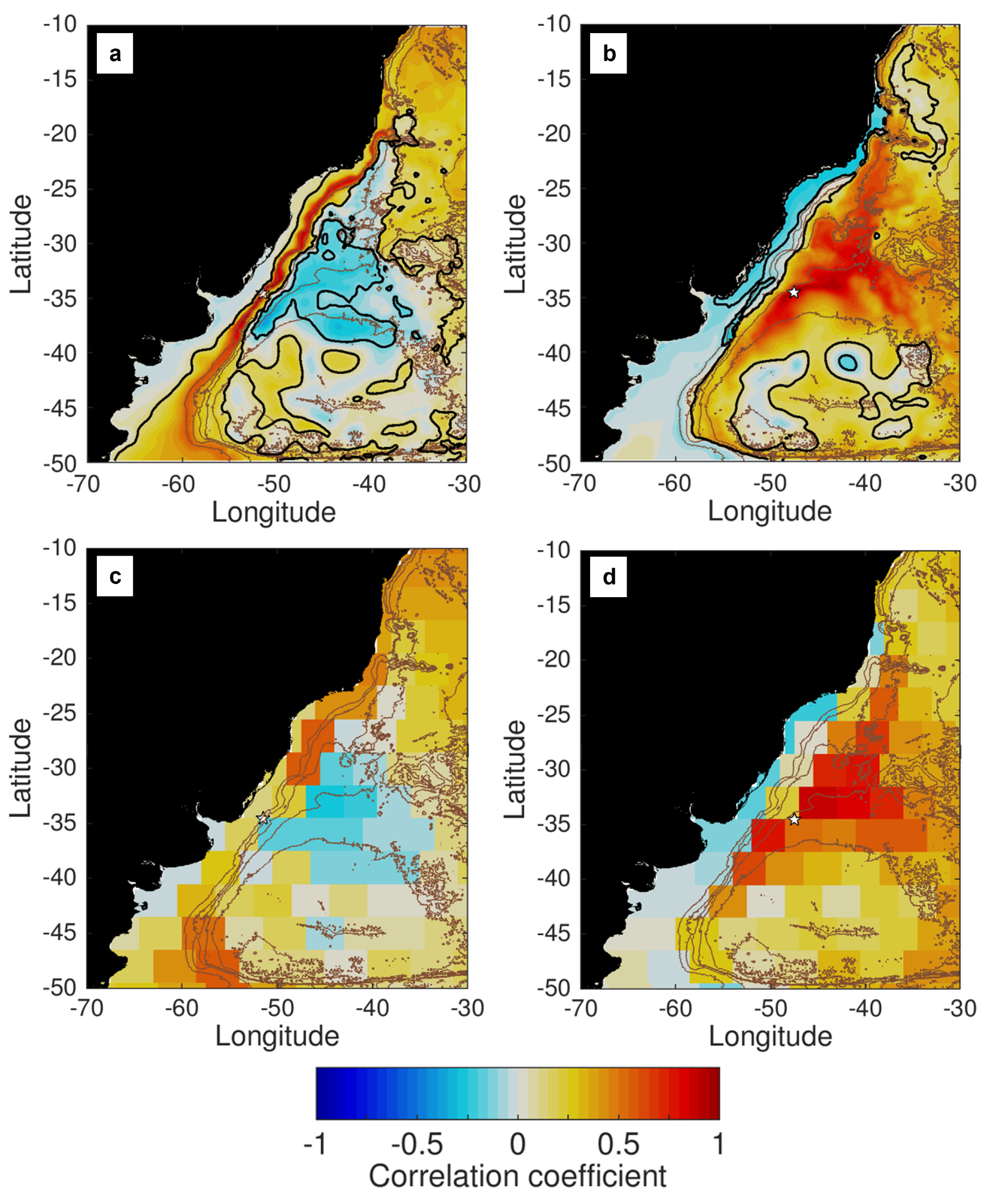
Within the context of the model-based objective reconstruction, a depth-based adjustment was applied to the point-mascon covariance vector to improve the resolution of OBP on steep continental slopes. In these boundary regions, OBP tends to be highly spatially correlated with points at a similar depth along the same boundary (Figure 1). Much of this depth-dependence on OBP is already captured in the CS510 simulation, but is likely still underrepresented due to the limits of model grid spacing and spatial interpolation, especially in regions where the continental slope is less than 50 km (∼2 grid points) wide. The depth adjustment increases the spatial correlation and covariance for point-mascon pairs at similar depths, and is computed with the adjusted covariance vector :
with the entries in the adjustment vector given by:
where is the maximum adjustment to the correlation (when the average mascon depth is the same as at point d), and are the OBP standard deviations of mascon i and point d, respectively, and are the mean ocean depth in mascon i and the depth at point d, respectively, and is the maximum depth difference between mascon and point, beyond which no adjustment is applied. The free parameters and were set to and as these parameters yielded the most correlation improvement in the validation.
As a key focus of this study is to validate the downscaled GRACE OBP against in situ data, most of the ensuing analysis is restricted to variability in the 3–12 month frequency range (intraannual timescales). This restriction is forced by the limited time resolution of the GRACE data product (monthly averages), as well as the drift in bottom pressure sensors, which inhibits their ability to observe interannual variability, e.g., [11]. All time series (GRACE, model, and in situ BPR) had long-term trends and the annual cycle removed, and were bandpassed for 3–12 month frequencies using an error-function filter in the frequency domain, e.g., [39,40]. Moreover, the validation analysis was restricted to sites located near a steep bathymetric slope; this was done by fitting a plane to the 2-min resolution bathymetry [41] in a radius equivalent to 6 latitude distance around each point. Only sites where the planar fit spanned > 2000 m depth in this 6 radius circle, and where at least 2 years of in situ BPR data were available, were included in this assessment.
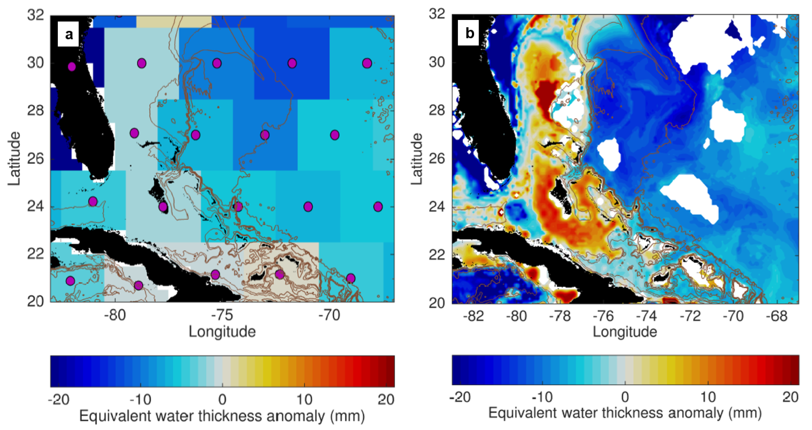
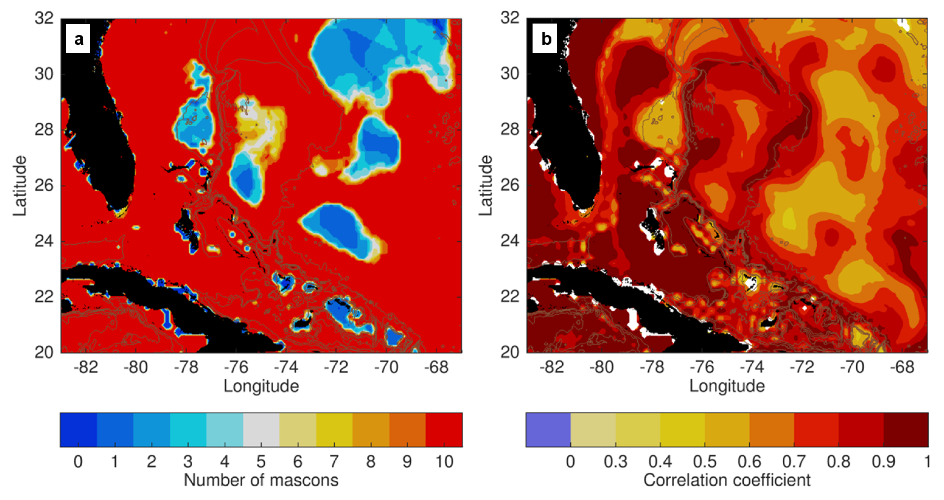
A demonstration of the downscaling procedure in the western Atlantic, applied to a particular month in the GRACE mascon dataset (Figure 2), illustrated the substantial change in OBP resolution that is possible. Whereas the mascon OBP consists of squares that span large ranges of ocean depth, the downscaled OBP has sharp gradients across the steep bathymetry of the continental slope east of the Bahamas, and also across the path of the Gulf Stream south and east of Florida. It seems probable that the downscaled OBP values are too positive in the shallow ocean plateau surrounding the Bahamas, but elsewhere, the values are in broad agreement with the mascons in the same region, other than the gradients near bathymetry changes. For most points, there were 10 mascons available to be used in the downscaling procedure (Figure 3a). At points where fewer or no mascons met the minimum correlation criterion (corr > 0.3), a model analysis suggested that the downscaled OBP had lower correlations with the true OBP at that point (Figure 3b). The correlation map in Figure 3b also indicated generally high correlations along the continental slope areas (e.g., east of the Bahamas), though this assumes that model correlation statistics with synthetic mascons are representative of the true correlations, which may not be the case.
3. Results
3.1. Validation with In Situ BPR Data
To assess the effect of the downscaling procedure and the depth adjustment on the accuracy of OBP estimates, the intraannual-filtered time series at the 43 BPR sites were correlated with (1) the not-downscaled (i.e., co-located GRACE JPL mascon) time series, (2) the downscaled time series with the covariance vector defined based on the model covariance only (), and (3) the downscaled time series with the depth adjustment described in Equations (3) and (4). By taking the differences in the correlation coefficient between when the downscaled time series are used vs. the not-downscaled time series, the added accuracy provided by the downscaling procedure could be quantified. Table 1 shows that correlations were improved at 28 of 43 sites (65%) using the model covariances only. With the depth adjustment, the correlations were improved at 34 of 43 sites (79%); 15 of these 43 sites (35%) had correlations improved by greater than 0.05. For a not-downscaled correlation value of 0.3 (approximately the median), a correlation improvement of 0.05 increased the variance explained by 36%.
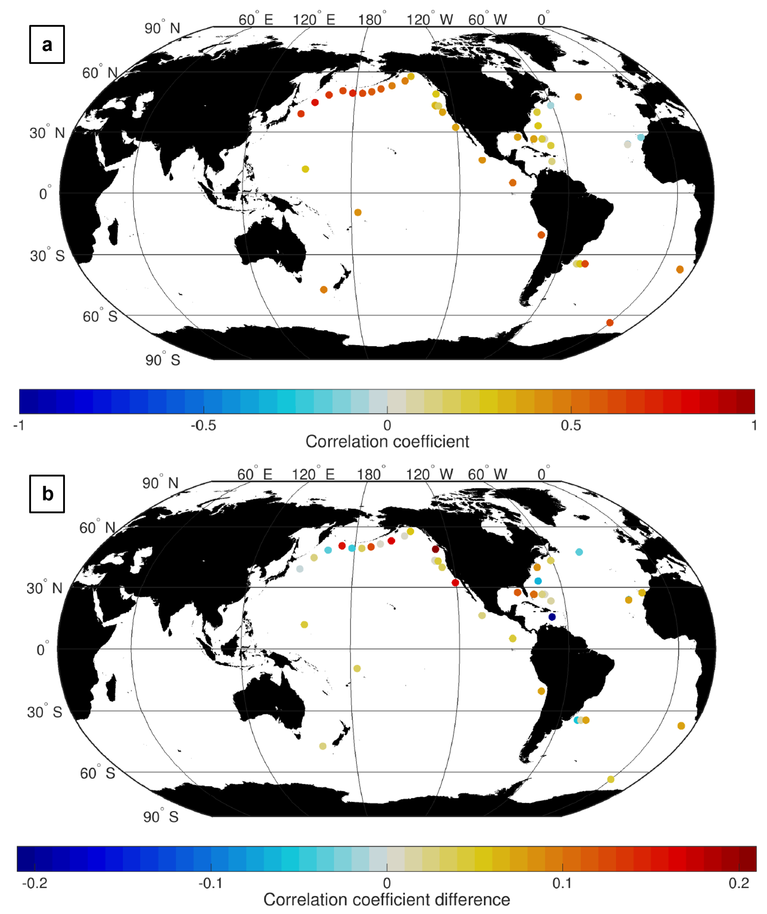
Intraannual correlations between the in situ BPR and the depth-adjusted downscaled GRACE were strongly positive (>0.5) in the northwest Pacific (Figure 4a), with some strongly positive correlations also present in the (more data-sparse) south Pacific and south Atlantic. The weakest correlations were found in the north Atlantic, as well as the northeastern Pacific near the coasts of Oregon and Washington. Regarding correlation improvements compared to the not-downscaled time series, there is no discernible geographic pattern (Figure 4b); substantial improvements in correlation are found at sites in the north Pacific as well as the north and south Atlantic, but each of these regions also has sites where the correlation with in situ data was not improved (or decreased) by the downscaling procedure.
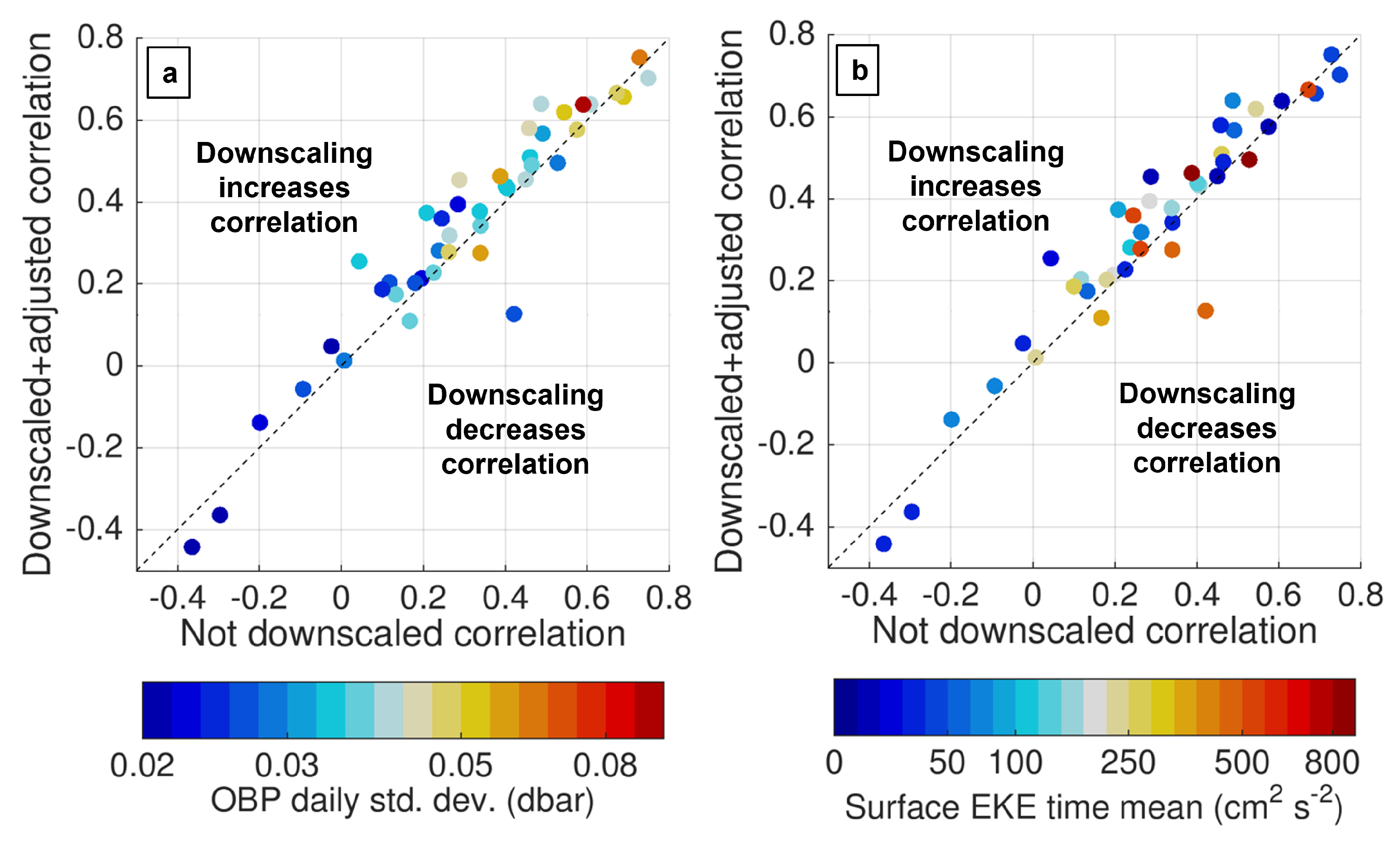
When correlation improvements are considered as a function of other site properties, some patterns are apparent. At sites where the amplitude of daily-averaged OBP (including all timescales from synoptic to interannual) is larger, the in situ OBP at intraannual timescales is generally more highly correlated with both not-downscaled and downscaled/adjusted GRACE (Figure 5a). This may imply that sites with lower OBP amplitudes are noisier and more difficult to estimate using the downscaling method. Notably, the amplitude of OBP variability at intraannual-only timescales has no apparent relationship to the correlations, suggesting that the relationship indicated in Figure 5a is associated with the leakage of noise from other timescales.
Given the resolution limitations of the existing GRACE mascon product, the spatial and temporal aliasing of mesoscale instabilities may also be an impediment to the downscaling of GRACE OBP. Of the nine sites where the correlation decreased with the downscaling, five had a relatively large surface EKE of >300 cm s (Figure 5b). While some other sites with high EKE did have correlations improved with downscaling, there was a higher probability that a correlation would not be improved if EKE is relatively high. Hence, Figure 5 indicates that accurate results are more likely in locations where the amplitude of the OBP signal is higher, but where EKE and mesoscale activity are lower.
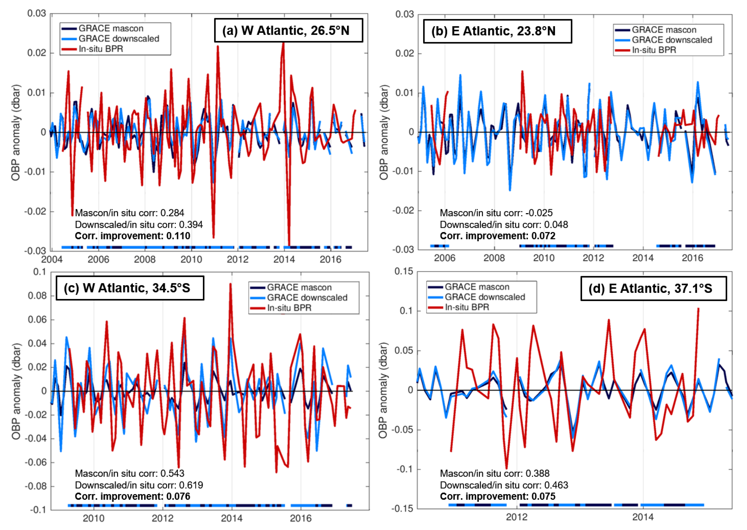
Time series comparisons of OBP at a few of the validation sites demonstrate how downscaling may improve correlation with in situ BPR time series at sites near deep ocean boundaries (Figure 6), while not improving the OBP estimate in a clear majority of times. All of the sites shown have an improvement in correlation; yet, in each time series, there are many times when the not-downscaled mascon OBP is closer to the in situ OBP value than the downscaled OBP is. This is particularly evident in the NE Atlantic time series at 23.8N (Figure 6b), where a majority of times are better estimated by the co-located mascon OBP rather than the downscaled OBP; despite a nominal correlation improvement of 0.072, at this site, the correlations of both GRACE-derived time series with in situ OBP were near zero, consistent with [11], which also found weak correlations between GRACE and in situ OBP in the same region. The other sites also had a number of times when the mascon OBP estimate was closer to the in situ value; this may imply that the correlation improvement results not from consistent adjustment of the time series towards the in situ value, but from generally larger differences between the GRACE-derived timeseries when the downscaled time series is closer vs. when the not-downscaled mascon time series is closer.
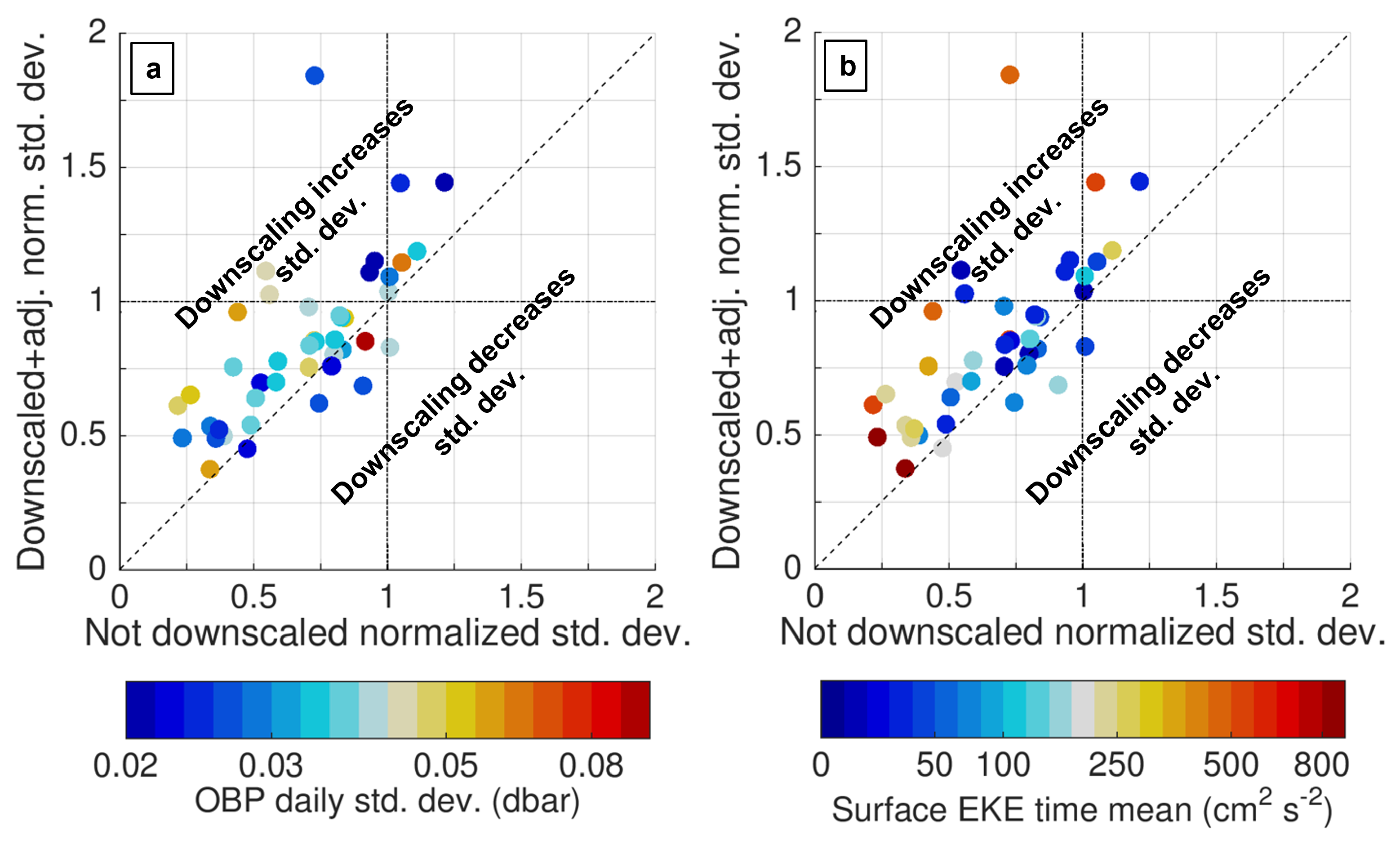
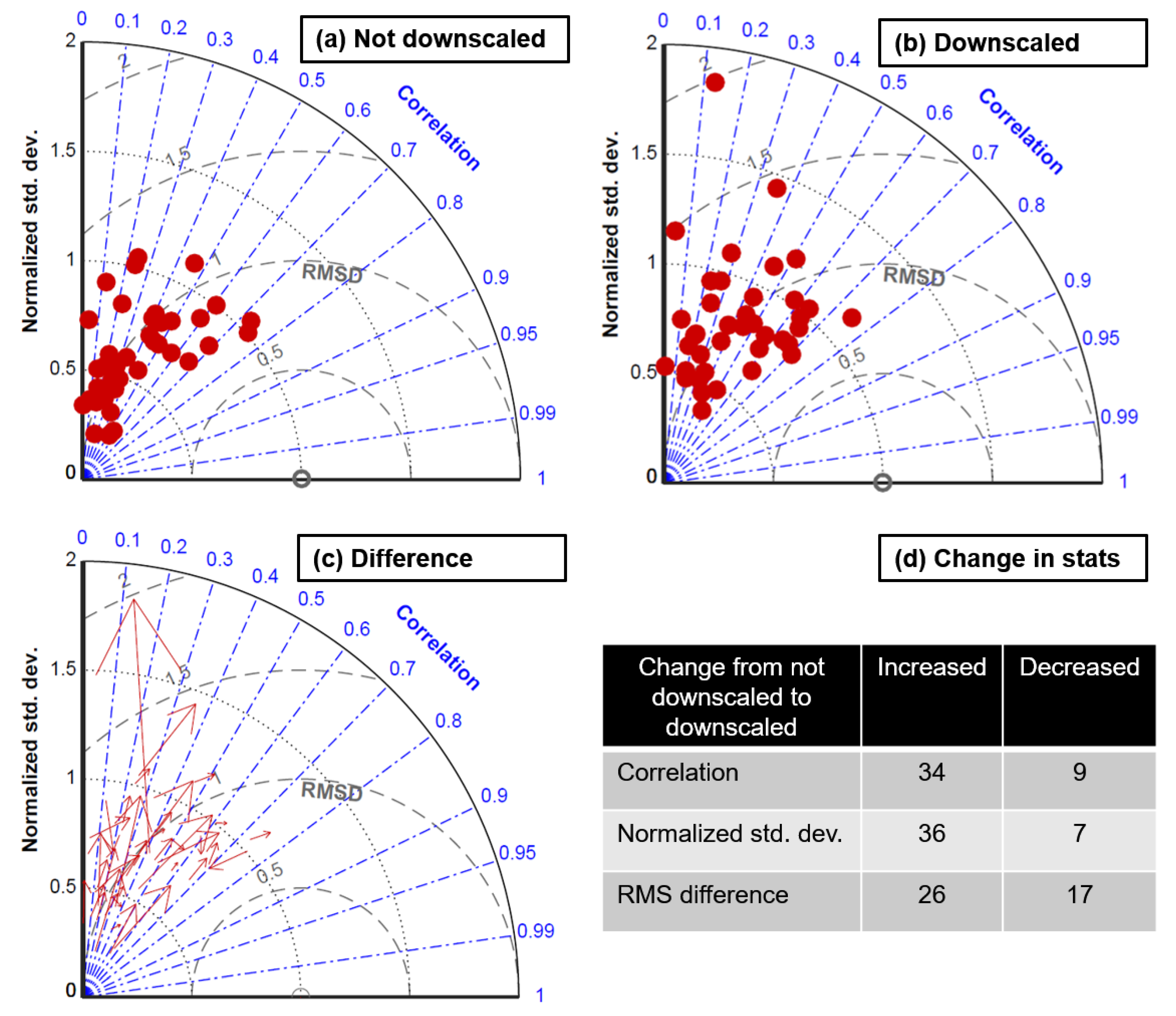
Some of the challenge in reducing the GRACE/in situ difference may be due to the increased OBP amplitudes in downscaled vs. not-downscaled time series. Figure 7 indicates that most not-downscaled OBP estimates have normalized standard deviations (NSD) less than 1 (are on the left side of the plot), i.e., the mascon OBP generally has smaller standard deviations than in situ observed OBP. However, downscaled GRACE OBP tends to increase standard deviations relative to not-downscaled GRACE, as indicated by most circles being to the left of the diagonal dashed line in Figure 7a,b. Most sites with high daily standard deviations (Figure 7a) and high surface EKE values (Figure 7b) have not-downscaled NSD < 0.5, implying that GRACE mascon OBP significantly underestimates the amplitude of local OBP variability, perhaps due to resolution limitations. The downscaling procedure increases NSD values at all sites where unfiltered standard deviation > 0.04 dbar, surface EKE > 300 cm s, and not-downscaled NSD < 0.5, bringing NSD values closer to 1 and therefore more realistic. The downside is that, even though the downscaling procedure increases correlations with in situ data at most sites, the increase in standard deviations results in increased root-mean-square difference (RMSD) between downscaled GRACE and in situ data (Figure 8).
3.2. Validation with RAPID Meridional Transport
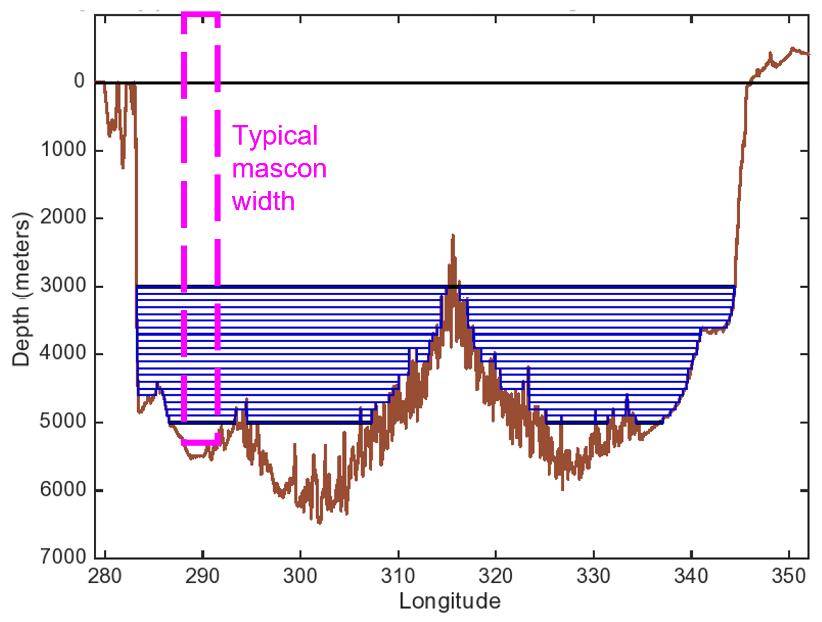
The primary motivation for the downscaling procedure is to improve OBP estimates near boundaries for the purposes of tracking meridional mass/volume transport. In this section, we use downscaled point OBP to estimate meridional transport variability in the deep Atlantic across 26.5N, and compare this estimate with the in situ hydrography-based RAPID transport time series. Figure 9 indicates how this calculation was carried out. The depth layer where the transport is calculated (3000–5000 m) was divided into bins of depth thickness 100 m each. At these depths, the Mid-Atlantic Ridge bisects the basin, so each 100 m depth bin was further divided into two segments, one each on the western and eastern sides of the ridge. The downscaling procedure was applied to obtain an OBP estimate at the endpoint of each segment. Following [3,9], the transport in each segment was obtained by differencing the OBP at the endpoints and integrating vertically, based on a zonal integration of the geostrophic relation:
where is the thickness of the depth bin and and are the pressure anomalies at the eastern and western ends of each segment. The sum of the segments at all depth levels is the transport anomaly in the 3000–5000 m depth layer.
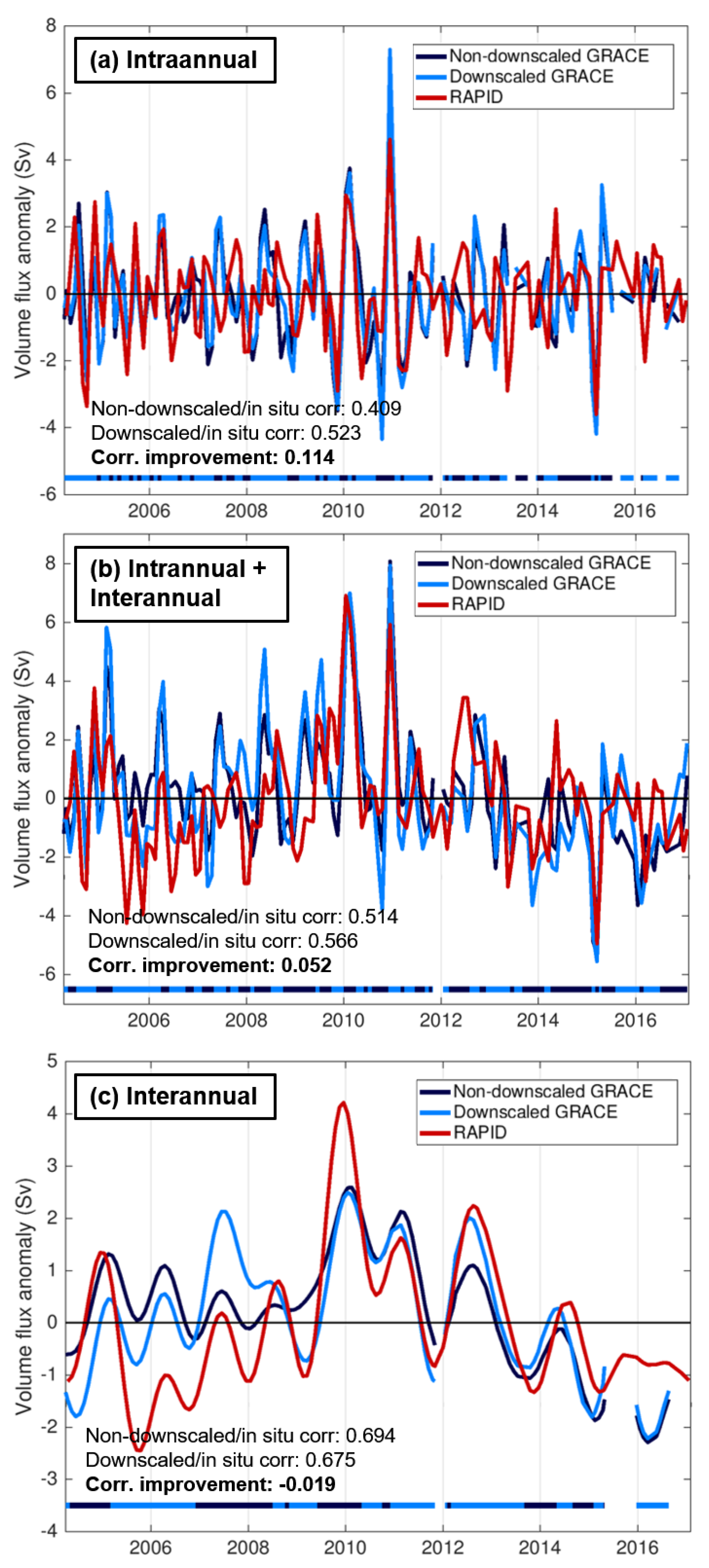
The comparison of Atlantic deep ocean transport estimates from GRACE with RAPID at intraannual timescales (Figure 10a) implies substantial improvement in the transport estimate associated with the downscaling procedure. The improvement is most apparent in the time series prior to 2012, and in particular in the first three years (2004–2006) of the time series where the downscaled GRACE-based estimate is consistently in phase with RAPID. The correlation improvement in the transport estimate (0.114) was also very similar to the correlation improvement in the point OBP estimate at the western boundary (Figure 6a), consistent with the transport variability at this transect being dominated by the western boundary variability [9,11].
Unlike the in situ BPRs, which are subject to spurious drifts over the course of a deployment, the RAPID transport time series is based on hydrographic observations of temperature and salinity (and hence density), which can be reliably used to study variability on longer interannual timescales. Though the spatial covariances in Equation (1) are based on intraannual frequencies, they have been used to compute downscaled time series at interannual timescales as well, in part to test how well intraannually-derived covariances can be applied to longer timescales. The application to the Atlantic 26.5N transect implies that using the intraannual covariances at interannual timescales may not be successful. When the combined intraannual and interannual time series are compared (Figure 10b), the downscaling still provides some improvement, but it is reduced compared to the intraannual-only time series. When the time series are filtered for interannual timescales only, the downscaling does not provide any improvement overall (Figure 10c). Substantial improvements during 2011–2013 are offset by a positive bias in the downscaled time series during 2005–2008, after a large negative (southward) shift in the RAPID time series in 2005 is not represented in the downscaled time series.
4. Discussion
The downscaling of GRACE data with the aid of numerical model simulations offers the possibility of studies of deep ocean variability derived from satellites. Figure 2 illustrates how model-based covariances can enhance the depiction of GRACE OBP anomalies across bathymetry gradients and major currents. Compared to earlier filtering methods that used global or basin-wide EOFs [15,16], this method focuses on the most relevant variability within a given radius of any point (20). Compared with the pattern filtering method of [14], this method has a lower correlation threshold (0.3 vs. 0.7) to encompass a broader range of variability, and the objective technique used here removes the pattern-filtering bias towards signals that cover larger areas. The depth adjustment described in Equations (3) and (4) improves the effectiveness of the downscaling method, most likely by compensating for some of the blurring of variability across depth ranges that happens when interpolating from the already-interpolated 1/4 model output grid. Figure 4 shows that GRACE/in situ correlations tend to be higher in some regions (NW Pacific, S Atlantic) than in others (NE Pacific, N Atlantic), but there are no clear regional patterns where the downscaling method provides more improvement; this finding is consistent with a similar analysis of the pattern-filtering method in [14].
Figure 5 indicates some criteria by which better OBP estimates may be obtained from downscaled GRACE, while alluding to some potential impediments to accurate downscaling near boundaries. Figure 5a implies that accurate remotely-sensed OBP is more likely where the signal of OBP variability is large; conversely, where the OBP signal is smaller, the signal/noise ratio is likely smaller, and hence, the GRACE observations and model covariances are both more likely to be distorted by errors. Another source of uncertainty in the coarse-resolution GRACE products are OBP contributions from mesoscale activity, which Figure 5b implies can reduce the effectiveness of the downscaling procedure. The activity of mesoscale eddies is challenging to represent in spatial covariances derived from the model, because eddies can take different shapes and move in different directions, and the spatial scales of mesoscale eddies are similar to or smaller than the JPL GRACE mascons. Ref. [20] note that the OBP along basin boundaries is less subject to mesoscale activity than sea surface height is, but mesoscale activity in regions of energetic currents (e.g., the Gulf Stream extension, Antarctic Circumpolar Current) can still be large compared to other signals (large-scale gyre variations, coastally-trapped waves) that are better represented in model covariances. Much of the benefit of the downscaling procedure results from using distant but well-correlated mascon signals to improve the OBP estimate, which is impeded by the small-scale local signals of mesoscale activity.
One inference from Figure 5, Figure 6, Figure 7 and Figure 8 is that the downscaling procedure may produce improved correlations with in situ time series and more realistic OBP amplitudes, without reducing RMS differences or differences between GRACE-based and in situ OBP values during individual months. Moreover, even though the resolution of OBP appears to be substantially enhanced by downscaling (Figure 2), the accuracy of the downscaled OBP field is still limited by the spatial and temporal resolution of GRACE monitoring, and of model representations of the deep ocean at the timescales being studied. This study’s focus on intraannual timescales is a consequence of GRACE’s limited ability to resolve shorter (i.e., synoptic) timescales, combined with the spurious drifts of in situ BPRs that may distort longer interannual timescales. The accuracy of the GRACE mascon product depends on the model-based removal of diurnal/semidiurnal tides [42] and synoptic variations [43] that may be large compared to the intraannual signal. OBP in this frequency range is also more difficult for ocean models to predict than at synoptic timescales, e.g., [17], likely due to mesoscale activity, which may impact not only predictions of OBP phase but also model-based spatial covariance estimates.
Two possible avenues to improve the accuracy of downscaled GRACE products include: (1) a model-based process study that enhances knowledge of the major processes influencing boundary OBP at timescales resolved by GRACE/GRACE-FO, and (2) a study of alongtrack range acceleration across continental slopes where OBP signals are known to be large and vary considerably with depth. The first approach would use models to assess the relative dominance of processes in a given boundary region, and develop metrics to assess their activity in satellite gravimetry, altimetry, and other datasets. The second approach would identify GRACE tracks that cross a continental slope where OBP signals are particularly large and sufficiently removed from large land-based hydrology signals, so that knowledge of the “footprint” of the gravity signal in anisotropic continental slope regions can be constrained by data. These efforts would both help to improve the resolution of satellite gravimetry data near ocean basin boundaries, by liberating OBP observations from the mascon and spherical harmonic geometries, and instead analyzing the observations in the context of ocean bathymetry and dynamic processes.
Author Contributions
Conceptualization, A.D. and F.L.; methodology testing and refinement, A.D.; validation analysis, A.D.; writing—original draft preparation, A.D.; writing—review and editing, A.D. and F.L.; visualization, A.D.; supervision and project administration, F.L.; funding acquisition, F.L. All authors have read and agreed to the published version of the manuscript.
Funding
This research was carried out in part at the Jet Propulsion Laboratory, California Institute of Technology, under a contract with the National Aeronautics and Space Administration (NASA). The work has been supported/funded by NASA WBS 953005.02.01.01.62.
Data Availability Statement
The JPL GRACE mascon data presented in this study are available from the Physical Oceanography Distributed Active Archive Center (https://podaac.jpl.nasa.gov, accessed on 19 May 2019); access the latest version of the data through https://grace.jpl.nasa.gov, accessed on 19 May 2019 [21]. ECCO2 CS510 model output interpolated to a 1/4-degree grid is available through ECCO Drive (https://ecco.jpl.nasa.gov/drive/files/ECCO2/cube92_latlon_quart_90S90N/, accessed on 9 November 2019). The satellite altimetry product used to assess eddy kinetic energy is available through the Copernicus Marine Service (https://resources.marine.copernicus.eu/product-detail/SEALEVEL_GLO_PHY_L4_REP_\OBSERVATIONS_008_047, accessed on 28 November 2017). In situ data products are available as follows: DART BPR data from NOAA NCEI (https://www.ngdc.noaa.gov/hazard/DARTData.shtml accessed on 19 October 2020), RAPID BPR data from the British Oceanographic Data Centre (https://www.bodc.ac.uk/data/ accessed on 18 June 2021), Atlantic 34.5S PIES from NOAA AOML (https://www.aoml.noaa.gov/phod/research/moc/samoc/sam/data_access.php accessed 6 June 2019), Southern Ocean PIES data from Zenodo (https://zenodo.org/record/3549812 accessed on 7 June 2021), and 47N western Atlantic mooring data from PANGAEA (https://doi.pangaea.de/10.1594/PANGAEA.903211 accessed on 9 June 2021). RAPID hydrography-based transport estimates [35] can be obtained from https://rapid.ac.uk/rapidmoc/rapid_data/datadl.php accessed on 23 May 2019.
Acknowledgments
The authors acknowledge the use of computing resources provided by Tong Lee at the Jet Propulsion Laboratory to help carry out the analysis.
Conflicts of Interest
The authors declare no conflict of interest.
References
- Talley, L.D. Shallow, intermediate, and deep overturning components of the global heat budget. J. Phys. Oceanogr. 2003, 33, 530–560. [Google Scholar] [CrossRef]
- Johns, W.E.; Baringer, M.O.; Beal, L.; Cunningham, S.; Kanzow, T.; Bryden, H.L.; Hirschi, J.; Marotzke, J.; Meinen, C.; Shaw, B.; et al. Continuous, array-based estimates of Atlantic Ocean heat transport at 26.5∘N. J. Clim. 2011, 24, 2429–2449. [Google Scholar] [CrossRef] [Green Version]
- Mazloff, M.R.; Boening, C. Rapid variability of Antarctic Bottom Water transport into the Pacific Ocean inferred from GRACE. Geophys. Res. Lett. 2016, 43, 3822–3829. [Google Scholar] [CrossRef]
- Cunningham, S.A.; Kanzow, T.; Rayner, D.; Baringer, M.O.; Johns, W.E.; Marotzke, J.; Longworth, H.R.; Grant, E.M.; Hirschi, J.J.M.; Beal, L.M.; et al. Temporal variability of the Atlantic meridional overturning circulation at 26.5 N. Science 2007, 317, 935–938. [Google Scholar] [CrossRef] [Green Version]
- Frajka-Williams, E.; Ansorge, I.J.; Baehr, J.; Bryden, H.L.; Chidichimo, M.P.; Cunningham, S.A.; Danabasoglu, G.; Dong, S.; Donohue, K.A.; Elipot, S.; et al. Atlantic meridional overturning circulation: Observed transport and variability. Front. Mar. Sci. 2019, 6, 260. [Google Scholar] [CrossRef] [Green Version]
- Send, U.; Lankhorst, M.; Kanzow, T. Observation of decadal change in the Atlantic meridional overturning circulation using 10 years of continuous transport data. Geophys. Res. Lett. 2011, 38, L24606. [Google Scholar] [CrossRef] [Green Version]
- Meinen, C.S.; Speich, S.; Perez, R.C.; Dong, S.; Piola, A.R.; Garzoli, S.L.; Baringer, M.O.; Gladyshev, S.; Campos, E.J. Temporal variability of the meridional overturning circulation at 34.5∘S: Results from two pilot boundary arrays in the South Atlantic. J. Geophys. Res. Ocean. 2013, 118, 6461–6478. [Google Scholar] [CrossRef] [Green Version]
- Lozier, M.S.; Bacon, S.; Bower, A.S.; Cunningham, S.A.; De Jong, M.F.; De Steur, L.; Deyoung, B.; Fischer, J.; Gary, S.F.; Greenan, B.J.; et al. Overturning in the Subpolar North Atlantic Program: A new international ocean observing system. Bull. Am. Meteorol. Soc. 2017, 98, 737–752. [Google Scholar] [CrossRef] [Green Version]
- Landerer, F.W.; Wiese, D.N.; Bentel, K.; Boening, C.; Watkins, M.M. North Atlantic meridional overturning circulation variations from GRACE ocean bottom pressure anomalies. Geophys. Res. Lett. 2015, 42, 8114–8121. [Google Scholar] [CrossRef]
- Bergmann, I.; Dobslaw, H. Short-term transport variability of the Antarctic Circumpolar Current from satellite gravity observations. J. Geophys. Res. Ocean. 2012, 117, C05044. [Google Scholar] [CrossRef] [Green Version]
- Worthington, E.L.; Frajka-Williams, E.; McCarthy, G.D. Estimating the deep overturning transport variability at 26∘N using bottom pressure recorders. J. Geophys. Res. Ocean. 2019, 124, 335–348. [Google Scholar] [CrossRef] [Green Version]
- Kelly, K.A.; Thompson, L.; Lyman, J. The coherence and impact of meridional heat transport anomalies in the Atlantic Ocean inferred from observations. J. Clim. 2014, 27, 1469–1487. [Google Scholar] [CrossRef]
- Koelling, J.; Send, U.; Lankhorst, M. Decadal strengthening of interior flow of North Atlantic Deep Water observed by GRACE satellites. J. Geophys. Res. Ocean. 2020, 125, e2020JC016217. [Google Scholar] [CrossRef]
- Böning, C.; Timmermann, R.; Macrander, A.; Schröter, J. A pattern-filtering method for the determination of ocean bottom pressure anomalies from GRACE solutions. Geophys. Res. Lett. 2008, 35, L18611. [Google Scholar] [CrossRef] [Green Version]
- Chambers, D.P.; Willis, J.K. Analysis of large-scale ocean bottom pressure variability in the North Pacific. J. Geophys. Res. Ocean. 2008, 113, C11003. [Google Scholar] [CrossRef] [Green Version]
- Chambers, D.P.; Willis, J.K. A global evaluation of ocean bottom pressure from GRACE, OMCT, and steric-corrected altimetry. J. Atmos. Ocean. Technol. 2010, 27, 1395–1402. [Google Scholar] [CrossRef] [Green Version]
- Poropat, L.; Dobslaw, H.; Zhang, L.; Macrander, A.; Boebel, O.; Thomas, M. Time variations in ocean bottom pressure from a few hours to many years: In situ data, numerical models, and GRACE satellite gravimetry. J. Geophys. Res. Ocean. 2018, 123, 5612–5623. [Google Scholar] [CrossRef]
- Watkins, M.M.; Wiese, D.N.; Yuan, D.N.; Boening, C.; Landerer, F.W. Improved methods for observing Earth’s time variable mass distribution with GRACE using spherical cap mascons. J. Geophys. Res. Solid Earth 2015, 120, 2648–2671. [Google Scholar] [CrossRef]
- Wiese, D.N.; Landerer, F.W.; Watkins, M.M. Quantifying and reducing leakage errors in the JPL RL05M GRACE mascon solution. Water Resour. Res. 2016, 52, 7490–7502. [Google Scholar] [CrossRef]
- Hughes, C.W.; Williams, J.; Blaker, A.; Coward, A.; Stepanov, V. A window on the deep ocean: The special value of ocean bottom pressure for monitoring the large-scale, deep-ocean circulation. Prog. Oceanogr. 2018, 161, 19–46. [Google Scholar] [CrossRef]
- Wiese, D.N.; Yuan, D.N.; Boening, C.; Landerer, F.W.; Watkins, M.M. JPL GRACE Mascon Ocean, Ice, and Hydrology Equivalent Water Height Release 06 Coastal Resolution Improvement (CRI) Filtered Version 1.0. Available online: https://podaac.jpl.nasa.gov/dataset/TELLUS_GRACE_MASCON_CRI_GRID_RL06_V1 (accessed on 19 May 2019). [CrossRef]
- Bentel, K.; Landerer, F.W.; Boening, C. Monitoring Atlantic overturning circulation and transport variability with GRACE-type ocean bottom pressure observations—A sensitivity study. Ocean. Sci. 2015, 11, 953–963. [Google Scholar] [CrossRef] [Green Version]
- Swenson, S.; Chambers, D.; Wahr, J. Estimating geocenter variations from a combination of GRACE and ocean model output. J. Geophys. Res. Solid Earth 2008, 113, B08410. [Google Scholar] [CrossRef] [Green Version]
- Peltier, R.W.; Argus, D.F.; Drummond, R. Comment on “An assessment of the ICE-6G_C (VM5a) glacial isostatic adjustment model” by Purcell et al. J. Geophys. Res. Solid Earth 2018, 123, 2019–2028. [Google Scholar] [CrossRef]
- Marshall, J.; Adcroft, A.; Hill, C.; Perelman, L.; Heisey, C. A finite-volume, incompressible Navier Stokes model for studies of the ocean on parallel computers. J. Geophys. Res. Ocean. 1997, 102, 5753–5766. [Google Scholar] [CrossRef] [Green Version]
- Menemenlis, D.; Campin, J.M.; Heimbach, P.; Hill, C.; Lee, T.; Nguyen, A.; Schodlok, M.; Zhang, H. ECCO2: High resolution global ocean and sea ice data synthesis. Mercat. Ocean. Q. Newsl. 2008, 31, 13–21. [Google Scholar]
- Volkov, D.L.; Lee, T.; Fu, L.L. Eddy-induced meridional heat transport in the ocean. Geophys. Res. Lett. 2008, 35, L20601. [Google Scholar] [CrossRef] [Green Version]
- Menemenlis, D.; Hill, C.; Adcrocft, A.; Campin, J.M.; Cheng, B.; Ciotti, B.; Fukumori, I.; Heimbach, P.; Henze, C.; Köhl, A.; et al. NASA supercomputer improves prospects for ocean climate research. Eos Trans. Am. Geophys. Union 2005, 86, 89–96. [Google Scholar] [CrossRef]
- Menemenlis, D.; Fukumori, I.; Lee, T. Using Green’s functions to calibrate an ocean general circulation model. Mon. Weather. Rev. 2005, 133, 1224–1240. [Google Scholar] [CrossRef] [Green Version]
- Meinig, C.; Stalin, S.E.; Nakamura, A.I.; Milburn, H.B. Real-Time Deep-Ocean Tsunami Measuring, Monitoring, and Reporting System: The NOAA DART II Description and Disclosure; NOAA Pacific Marine Environmental Laboratory: Seattle, WA, USA, 2005; pp. 1–15. [Google Scholar]
- Elipot, S.; Hughes, C.; Olhede, S.; Toole, J. Coherence of western boundary pressure at the RAPID WAVE array: Boundary wave adjustments or deep western boundary current advection? J. Phys. Oceanogr. 2013, 43, 744–765. [Google Scholar] [CrossRef] [Green Version]
- Hughes, C.W.; Elipot, S.; Morales Maqueda, M.Á.; Loder, J.W. Test of a method for monitoring the geostrophic meridional overturning circulation using only boundary measurements. J. Atmos. Ocean. Technol. 2013, 30, 789–809. [Google Scholar] [CrossRef] [Green Version]
- Androsov, A.; Boebel, O.; Schröter, J.; Danilov, S.; Macrander, A.; Ivanciu, I. Ocean Bottom Pressure Variability: Can It Be Reliably Modeled? J. Geophys. Res. Ocean. 2020, 125, e2019JC015469. [Google Scholar] [CrossRef]
- Rhein, M.; Mertens, C.; Roessler, A. Observed transport decline at 47∘N, western Atlantic. J. Geophys. Res. Ocean. 2019, 124, 4875–4890. [Google Scholar] [CrossRef]
- Smeed, D.; McCarthy, G.; Rayner, D.; Moat, B.I.; Johns, W.E.; Baringer, M.O.; Meinen, C.S. Atlantic Meridional Overturning Circulation Observed by the RAPID-MOCHA-WBTS (RAPID-Meridional Overturning Circulation and Heatflux Array-Western Boundary Time Series) Array at 26N from 2004 to 2017; British Oceanographic Data Centre, Natural Environment Research Council: Liverpool, UK, 2017. [Google Scholar] [CrossRef]
- Kanzow, T.; Cunningham, S.A.; Rayner, D.; Hirschi, J.J.M.; Johns, W.E.; Baringer, M.O.; Bryden, H.L.; Beal, L.M.; Meinen, C.S.; Marotzke, J. Observed flow compensation associated with the MOC at 26.5∘N in the Atlantic. Science 2007, 317, 938–941. [Google Scholar] [CrossRef] [PubMed] [Green Version]
- McCarthy, G.D.; Smeed, D.A.; Johns, W.E.; Frajka-Williams, E.; Moat, B.I.; Rayner, D.; Baringer, M.O.; Meinen, C.S.; Collins, J.; Bryden, H.L. Measuring the Atlantic meridional overturning circulation at 26∘N. Prog. Oceanogr. 2015, 130, 91–111. [Google Scholar] [CrossRef] [Green Version]
- Ducet, N.; Le Traon, P.Y.; Reverdin, G. Global high-resolution mapping of ocean circulation from TOPEX/Poseidon and ERS-1 and-2. J. Geophys. Res. Ocean. 2000, 105, 19477–19498. [Google Scholar] [CrossRef]
- Delman, A.S.; Lee, T.; Qiu, B. Interannual to multidecadal forcing of mesoscale eddy kinetic energy in the subtropical southern Indian Ocean. J. Geophys. Res. Ocean. 2018, 123, 8180–8202. [Google Scholar] [CrossRef]
- Delman, A.; Lee, T. A new method to assess mesoscale contributions to meridional heat transport in the North Atlantic Ocean. Ocean. Sci. 2020, 16, 979–995. [Google Scholar] [CrossRef]
- Smith, W.H.; Sandwell, D.T. Global sea floor topography from satellite altimetry and ship depth soundings. Science 1997, 277, 1956–1962. [Google Scholar] [CrossRef] [Green Version]
- Ray, R.D. A Global Ocean Tide Model from TOPEX/POSEIDON Altimetry: GOT99. 2; National Aeronautics and Space Administration, Goddard Space Flight Center: Greenbelt, MD, USA, 1999. [Google Scholar]
- Dobslaw, H.; Bergmann-Wolf, I.; Dill, R.; Poropat, L.; Thomas, M.; Dahle, C.; Esselborn, S.; König, R.; Flechtner, F. A new high-resolution model of non-tidal atmosphere and ocean mass variability for de-aliasing of satellite gravity observations: AOD1B RL06. Geophys. J. Int. 2017, 211, 263–269. [Google Scholar] [CrossRef] [Green Version]
Figure 1.
(a) Correlation of OBP at 34.5S, 51.5W (∼1500 m depth) with OBP in the surrounding region in the ECCO2 CS510 simulation, bandpassed for 3–12 month timescales with the seasonal cycle removed. Thin brown contours indicate bathymetry at intervals of 1000 m; thick black contours indicate correlation significance at the 95% confidence level. (b) Same as (a) but for OBP correlation with 34.5S, 47.5W (∼4400 m depth). (c) Correlation of OBP at 34.5S, 51.5W with surrounding synthetic mascons, 3–12 month timescales, and (d) same but for correlation with 34.5S, 47.5W.

Figure 2.
(a) GRACE OBP anomaly (in units of equivalent water thickness anomaly) in the subtropical western Atlantic, March 2010, from the JPL RL06M mascon product bandpassed for 3–12 month timescales. Brown contours indicate bathymetry at intervals of 1000 m. (b) Same but for the downscaled GRACE OBP anomaly with depth adjustment. Areas without shading did not have at least 3 mascons in the set , as described in Section 2.2.

Figure 3.
(a) Number of mascons in the set used to produce downscaled OBP at each point. Brown contours indicate bathymetry at intervals of 1000 m. (b) Correlation coefficient of point OBP with OBP downscaled from synthetic mascon OBP in the ECCO2 CS510 simulation.
Figure 3.
(a) Number of mascons in the set used to produce downscaled OBP at each point. Brown contours indicate bathymetry at intervals of 1000 m. (b) Correlation coefficient of point OBP with OBP downscaled from synthetic mascon OBP in the ECCO2 CS510 simulation.

Figure 4.
(a) Correlation coefficient of depth-adjusted downscaled GRACE with in situ BPR time series, 3–12 month timescales. (b) Correlation coefficient difference between depth-adjusted downscaled GRACE correlations in (a), minus the correlations of not-downscaled GRACE with in situ BPR time series.

Figure 5.
Scatter plots of correlations between in situ and GRACE-based OBP, 3–12 month timescales. The x-axis indicates the correlation without downscaling of the GRACE data, the y-axis indicates the correlation with the depth-adjusted downscaled GRACE data, with the dashed diagonal line indicating zero improvement. Color shading of the circles indicates (a) the standard deviation of OBP at each site in daily averages from ECCO2 CS510 without further temporal filtering, and (b) the time mean surface eddy kinetic energy at the site, computed from gridded CMEMS altimetry data.

Figure 6.
Time series comparisons of in situ BPR time series with (non-downscaled) GRACE mascon OBP and downscaled GRACE OBP, filtered for 3–12 month timescales with temporal mean, trend, and seasonal cycle removed. The horizontal bars at the bottom of each plot (dark blue or light blue) indicate whether the absolute difference of |non-downscaled − in situ| (dark blue) or |downscaled − in situ| (light blue) is smaller. Locations of each site are (a) 26.51N, 76.74W, 3700 m depth, (b) 23.8N, 24.1W, 5100 m depth, (c) 34.5S, 44.5W, 4800 m depth, and (d) 37.1S, 12.8W, 4900 m depth.

Figure 7.
Scatter plots of standard deviations of not downscaled and downscaled+adjusted GRACE-based point OBPs, normalized by in situ BPR standard deviations at the same sites, 3–12 month timescales. The x-axis indicates the normalized standard deviation without downscaling of the GRACE data; the y-axis indicates the correlation with the depth-adjusted downscaled GRACE data. Color shading of the circles is according to (a) OBP daily standard deviations with no temporal filtering, and (b) surface EKE, following Figure 5.

Figure 8.
(a) Taylor diagram with red circles indicating the correlation and standard deviation of not downscaled (mascon) GRACE OBP with OBP from in situ BPRs, 3–12 month timescales, positive correlations only. The standard deviations were normalized by the in situ BPR standard deviations as in Figure 7. (b) Same as (a) but for the downscaled GRACE OBP values. (c) Diagram showing the difference (change) in correlation and normalized standard deviation due to the downscaling; the red vectors indicate the difference between not downscaled and downscaled values, pointing to the downscaled values. (d) Table indicating how many sites had an increase/decrease in correlation, normalized std. dev., and RMS difference with in situ OBP time series (among 43 total sites).

Figure 9.
Depth-longitude section of the transect across the Atlantic Ocean at 26.5N latitude. The brown line indicates the topography/bathymetry, and the magenta dashed rectangle the typical longitudinal width of a mascon in the JPL RL06M product. The blue rectangles indicate the bin segments (100 m depth each) used to compute the layer transport anomaly.

Figure 10.
Comparison of volume flux (transport) anomaly time series in the Atlantic across 26.5N, at 3000–5000 m depth. Horizontal bars at the bottom indicate which GRACE OBP value was closer to the RAPID value at that time, similarly to Figure 6. The time series are filtered for (a) 3–12 month timescales, (b) timescales > 3 months, and (c) timescales > 14 months; all time series have temporal mean, trend, and seasonal cycle removed.


Table 1.
Improvement in correlation coefficient with in situ BPR provided by the downscaling procedure without and with the depth adjustment, 3–12 month timescales.
Table 1.
Improvement in correlation coefficient with in situ BPR provided by the downscaling procedure without and with the depth adjustment, 3–12 month timescales.
| Number of Sites | ||
|---|---|---|
| Correlation Improvement | Model Cov. Only | Depth-Adjusted Cov. |
| <0 | 15 | 9 |
| 0–0.05 | 17 | 19 |
| 0.05–0.1 | 7 | 8 |
| 0.1–0.2 | 3 | 6 |
| >0.2 | 1 | 1 |
| Total sites | 43 | 43 |
| Total > 0 | 28 | 34 |
Publisher’s Note: MDPI stays neutral with regard to jurisdictional claims in published maps and institutional affiliations. |
© 2022 by the authors. Licensee MDPI, Basel, Switzerland. This article is an open access article distributed under the terms and conditions of the Creative Commons Attribution (CC BY) license (https://creativecommons.org/licenses/by/4.0/).
Share and Cite
MDPI and ACS Style
Delman, A.; Landerer, F. Downscaling Satellite-Based Estimates of Ocean Bottom Pressure for Tracking Deep Ocean Mass Transport. Remote Sens. 2022, 14, 1764. https://doi.org/10.3390/rs14071764
AMA Style
Delman A, Landerer F. Downscaling Satellite-Based Estimates of Ocean Bottom Pressure for Tracking Deep Ocean Mass Transport. Remote Sensing. 2022; 14(7):1764. https://doi.org/10.3390/rs14071764
Chicago/Turabian StyleDelman, Andrew, and Felix Landerer. 2022. "Downscaling Satellite-Based Estimates of Ocean Bottom Pressure for Tracking Deep Ocean Mass Transport" Remote Sensing 14, no. 7: 1764. https://doi.org/10.3390/rs14071764
Note that from the first issue of 2016, this journal uses article numbers instead of page numbers. See further details here.