Article

Global Spatiotemporal Variability of Integrated Water Vapor Derived from GPS, GOME/SCIAMACHY and ERA-Interim: Annual Cycle, Frequency Distribution and Linear Trends

1
Royal Meteorological Institute of Belgium (RMIB), 1180 Uccle, Belgium
2
Royal Observatory of Belgium (ROB), 1180 Uccle, Belgium
3
Department of Hydrology and Climatology, Faculty of Chemistry and Geosciences, Institute of Geosciences, Vilnius University, 01513 Vilnius, Lithuania
4
Max Planck Institute for Chemistry (MPI-C), 55128 Mainz, Germany
5
Royal Belgium Institute for Space Aeronomy (BIRA), 1180 Uccle, Belgium
6
Met Office, Exeter EX1 3PB, UK
*
Author to whom correspondence should be addressed.
Remote Sens. 2022, 14(4), 1050; https://doi.org/10.3390/rs14041050
Submission received: 23 December 2021 / Revised: 17 February 2022 / Accepted: 17 February 2022 / Published: 21 February 2022
(This article belongs to the Special Issue Climate Modelling and Monitoring Using GNSS)

Abstract

:
Atmospheric water vapor plays a prominent role in climate change and atmospheric, meteorological, and hydrological processes. Because of its high spatiotemporal variability, precise quantification of water vapor is challenging. This study investigates Integrated Water Vapor (IWV) variability for the period 1995–2010 at 118 globally distributed Global Positioning System (GPS) sites, using additional UV/VIS satellite retrievals by GOME, SCIAMACHY, and GOME-2 (denoted as GOMESCIA below), plus ERA-Interim reanalysis output. Apart from spatial representativeness differences, particularly at coastal and island sites, all three IWV datasets correlate well with the lowest mean correlation coefficient of 0.878 (averaged over all the sites) between GPS and GOMESCIA. We confirm the dominance of standard lognormal distribution of the IWV time series, which can be explained by the combination of a lower mode (dry season characterized by a standard lognormal distribution with a low median value) and an upper mode (wet season characterized by a reverse lognormal distribution with high median value) in European, Western American, and subtropical sites. Despite the relatively short length of the time series, we found a good consistency in the sign of the continental IWV trends, not only between the different datasets, but also compared to temperature and precipitation trends.

1. Introduction

Being the most important natural greenhouse gas, water vapor plays a crucial role in climate change. It is governed by temperature through the Clausius-Clapeyron equation which states that the capacity of the atmosphere to hold water vapor increases by 7% per degree Celsius increment in temperature [1,2,3,4]. At all scales, water vapor also strongly influences atmospheric dynamics and the hydrologic cycle through surface evaporation, latent heat transportation, and diabatic heating, and is, of course, a source of clouds and precipitation.
As atmospheric water vapor is highly variable in space and in time [5], its accurate measurement is extremely challenging. Atmospheric Integrated Water Vapor (IWV) may be measured using in situ instruments (e.g., radiosondes) or from space using instruments on board satellites. Guerova et al. [6] divided remote sensing techniques into three categories: (1) differential time of arrival measurements, such as GPS, (2) active techniques such as LIght Detection And Ranging (LIDAR) and RAdio Detection And Ranging (RADAR), and (3) passive techniques based on emission/absorption measurements, e.g., microwave radiometers [7,8]. Space-borne observations of IWV utilize different regions of the electromagnetic spectrum, from microwave to the thermal infrared. An inventory of many of the satellite techniques has been carried out within the Global Energy and Water Exchanges (GEWEX) Water Vapor Assessment (G-VAP) and is available online [9]. All IWV observation techniques have their advantages and disadvantages and have been compared in numerous previous studies (e.g., http://www.meteo.be/IWVintercomp, accessed on 21 December 2021, provides a literature review of past IWV inter-technique studies involving GNSS, and also see Vaquero-Martinez and Antón [10]). Van Malderen et al. [11] compared five different techniques and concluded that GPS and GOMESCIA can be used to study global inter-annual IWV variability.
Global mean IWV distribution correlates well with mean temperature and is highest in the tropics, where strong evaporation occurs and trade winds transport the high levels of moisture to the Intertropical Convergence Zone [12,13]. At mid and high latitudes, evaporation is weaker and lower IWV amounts are thus observed. Furthermore, the highest mean IWV values generally occur in summer, and conversely, the lowest IWV values occur in the cold, winter months. Foster et al. [14] studied the IWV frequency distribution at sites from various climatic regimes around the world. The lognormal distribution is commonly found in subtropical and temperate climates, while tropical oceanic environments have a reversed lognormal distribution. Bimodal distributions occur where seasonality is both pronounced and distinct, e.g., for monsoonal zones. Global decadal IWV trend studies (partly summarized until 2009 by Sherwood et al. [15] and thereafter in [12,13,16,17,18,19,20,21]) reveal a positive overall global mean trend, e.g., of 0.26, 0.24, and 0.34 mm dec−1, respectively, in the GPS (1995–2011), radiosonde (1973–2011), and microwave satellite (1988–2011) records [20]. However, the significance and sign of the trends change from region to region, between techniques, from dataset to dataset, and from study to study [17,19,22].
Therefore, in this paper, we investigate how well the spatial and temporal IWV variability are globally represented by three independent IWV datasets: two observational datasets (one ground-based and one satellite-based) and a numerical weather prediction model reanalysis output. By including three datasets using completely different IWV retrieval techniques and with different spatial and temporal resolutions, we attempt to create a consistent picture of global IWV spatiotemporal variability. A characterization of the spatial IWV variability is given by considering the geographical distribution of the IWV frequency distributions, a worldwide extension of the work by Foster et al. [14]. To assess the temporal IWV variability of the three datasets, we consider different time scales: from seasonal cycles to inter-annual variability and trends of periods up to 15 years.
This paper is organized as follows: Section 2 describes the observing techniques and methods used to retrieve IWV; Section 3 compares the IWV datasets (Section 3.1), studies seasonal behavior (Section 3.2), analyzes the geographical distribution of IWV frequency distributions (Section 3.3), and presents linear trends (Section 3.4); Section 4 is reserved for the discussion and outlook.

2. Datasets and Methodology
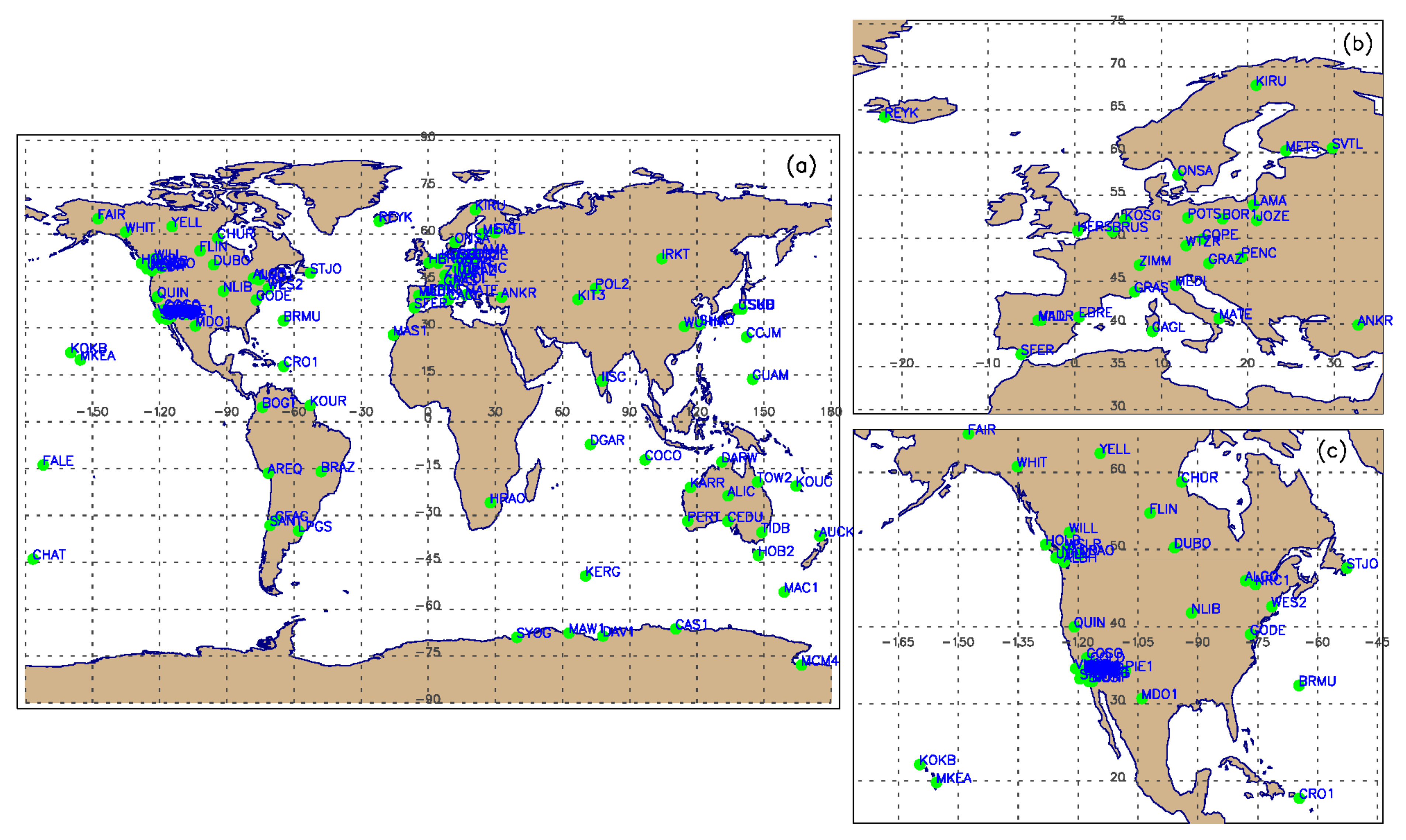
To study IWV variability, we use IWV retrievals from GPS continually observing reference stations (CORS), a merged dataset of IWV measured from 3 different satellite instruments (GOME, SCIAMACHY, GOME-2) and from the ERA-Interim [23] reanalysis model.

2.1. GPS

Radio signals transmitted by GPS satellites, received at the Earth’s surface, are delayed by atmospheric water vapor along the signal path (mostly located in the troposphere). Using observations from GPS CORS networks, the Zenith Total Delay (ZTD) can be calculated which provides an estimate of the signal delay due to the neutral atmosphere [24].
In this paper, we use homogenously reprocessed ZTD data provided by the International GNSS Service (IGS) [25] Repro1 campaign [26], available for about 400 GPS stations from 1995 until April 2011. From this worldwide dataset of almost continuous and homogeneously reprocessed ZTDs, we selected the 118 IGS stations having the longest time series (16 years—see Figure 1 and Table S1 of the supplementary material). Although homogeneously reprocessed, the IGS ZTD time series can still contain discontinuities or break points due to unreported or mis-modelled instrument changes or changes in the observation statistics [27,28]. While those remaining inhomogeneities might impact trend estimation [12], a statistical homogenization of this dataset is out of scope for this paper; a benchmark study of different break detection methods on synthetic datasets created from the same GPS and ERA-Interim IWV time series is presented in Van Malderen et al. [29].
If surface pressure Ps and the water vapor weighted mean temperature of the atmosphere, Tm, are known at the GPS site [24], ZTD may be converted into IWV. In this study, the surface pressure Ps at the GPS site is calculated from the surface pressure values of the four surrounding grid points from the European Centre for Medium-Range Weather Forecasts (ECMWF) ERA-Interim reanalysis (Section 2.3) by horizontal interpolation, weighted with the inverse distance to the GPS station. To account for the height difference between the GPS station and the ERA-Interim surface grid points, we use the hydrostatic and ideal gas equations to adjust surface pressure to the height of the GPS antenna. Other studies use ERA-Interim pressure level data to derive the pressure at the GPS station, e.g., [12,28], or synoptic stations in the vicinity of the GPS stations, e.g., [11,30]. Parracho [31] (their Figure 2.82) showed that surface pressure interpolated or extrapolated from pressure level data is relatively consistent with model surface pressure data, thus suggesting no significant biases are introduced when comparing data derived from either method.
Tm can be either (i) calculated from vertical profile data of temperature and humidity, e.g., provided by radiosondes or reanalyses, or (ii) estimated from surface temperature (Ts) observations using a linear empirical relationship (e.g., Bevis et al. [24]). In this paper, we used the ERA-Interim pressure level data of temperature and specific humidity from the four grid points surrounding the GPS station. These profiles are horizontally interpolated, with the inverse distance to the GPS station as a weighting methodology. As the vertical integration to retrieve Tm starts from the ERA-Interim surface grid points and continues higher up with the ERA-Interim pressure level data, a correction for the height difference between the GPS station and the ERA-Interim surface grid points is required for surface temperature and specific humidity data. For the temperature, we assume a standard temperature lapse rate of −6.5 K km−1 (typical for wet adiabatic conditions), and for the specific humidity adjustment, a constant dew point temperature depression (T−Tdew) with height [32].
The auxiliary meteorological data from ERA-Interim reanalysis are only available at 0, 6, 12, and 18 h UTC, as such, the converted GPS IWV dataset (using the ERA-Interim data for ZTD to IWV conversion) is also only available at these times. There do exist however a number of GPS ZTD data gaps with only 77% of data being available on average at this time resolution (data availability ranges from 45% to 98.5%).
The choice of the auxiliary meteorological parameters used for the ZTD to IWV conversion can clearly impact the resulting IWV values and trends. Therefore, in Appendix A, we compare GPS IWV values and trends estimated by using different sources of auxiliary meteorological parameters (ERA-Interim, NCEP/NCAR reanalysis, SYNOP stations) and different calculation methods of Tm (from the linear empirical relationship with the surface temperature as outlined above). We found that, averaged over all stations, the surface pressure has a larger impact on IWV values and trends (mean absolute difference of about 0.3 mm and 0.35 mm dec−1, respectively) than surface temperature and weighted mean temperature (<0.07 mm and 0.11 mm dec−1, respectively). The low values demonstrate that the GPS IWV dataset can be considered as independent of the chosen dataset for the auxiliary meteorological data, and hence, in particular, independent of ERA-Interim IWV used in this paper for comparison.
Finally, using >40 IWV measurements per month (i.e., 30% of the expected measurements), we calculated monthly mean IWV values.

2.2. GOME/SCIAMACHY/GOME-2

In this paper, we use the IWV “Climate” product from the European Space Agency (ESA) GOME-Evolution project, described in Beirle et al. [33]. It is provided as a monthly mean IWV 1° × 1° global grid from July 1995 to December 2015. For our study, we considered those monthly mean IWV time series at the pixels closest to the GPS stations. This “Climate” product merges the IWV retrievals from three satellite spectrometers in the red spectral range with the same differential optical absorption spectroscopy (DOAS) technique: Global Ozone Monitoring Experiment (GOME, July 1995–July 2011), the Scanning Imaging Absorption spectroMeter for Atmospheric CHartographY (SCIAMACHY, August 2002–March 2012), and GOME-2 (since January 2007). For simplicity, we will subsequently use the acronym “GOMESCIA” in this paper. The three satellites have a constant equatorial crossing time between 9 h 30 and 10 h 30 local time. Cloud effects impacting the IWV retrievals [11] are also treated consistently for the different sensors by deriving the information required for air-mass factor correction and cloud masking directly from the spectral analysis. Spatial consistency is obtained by merging SCIAMACHY and GOME-2 observations to the larger GOME pixel size (320 × 40 km2) and reducing the GOME-2 swath width to that of GOME and SCIAMACHY.
The GOME-SCIAMACHY-GOME-2 time series are additionally homogenized by correcting for the offsets determined during sensor overlap periods. When validated with GNSS and ERA-Interim, mean biases of −1.0 and −0.65 mm (RMS of 4.3 and 3.4 mm, respectively) were found [33]. This small dry bias in GOMESCIA is due to the fact that cloudy images have to be masked out for satellite IWV retrievals in the visible wavelength range. A temporal stability of about 1% per decade is achieved for the GOMESCIA climate product [33].

2.3. ERA-Interim Reanalysis Model

The third independent IWV dataset that we consider in this paper is the ERA-Interim surface IWV output. ERA-Interim [23] is a global numerical weather prediction model with 4-dimensional variational (4D-Var) data assimilation with a 12 h analysis window, giving a temporal resolution of 6 h. It is important to note that the data assimilation system of ERA-Interim does not include ground-based GNSS data. The spatial resolution of the dataset is approximately 80 km (0.75° × 0.75°) and contains 60 vertical pressure levels from the surface to 0.1 hPa.
The IWV values at the GPS station locations were horizontally interpolated from the IWV output at the nearest four surrounding ERA-Interim surface grid points and weighted according to the inverse distance to the GPS station. Because the height of the GPS stations does not usually correlate with the ERA-Interim model topography, a vertical interpolation of the ERA-Interim IWV to the GPS station height is required. In this paper, we follow the approach proposed by Hagemann et al. [34], in which the adjustment is obtained by numerical integration of the specific humidity (q) over the height difference between the GPS station and model surface with a constant dew point depression being assumed.
ERA-Interim surface fields are also used for the extraction of surface temperature and pressure time series at the GPS site locations. We also apply the same horizontal interpolation of the values from the four surrounding grid points and the altitude corrections as described in Section 2.1.

3. Results

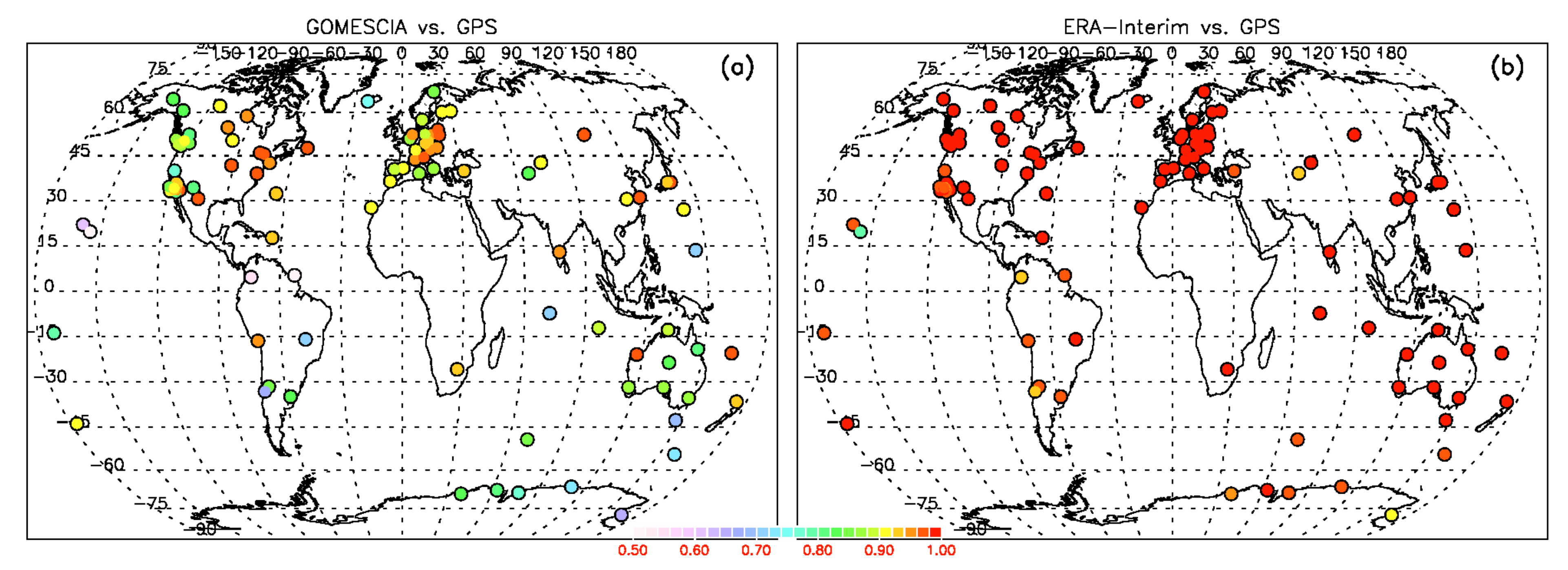
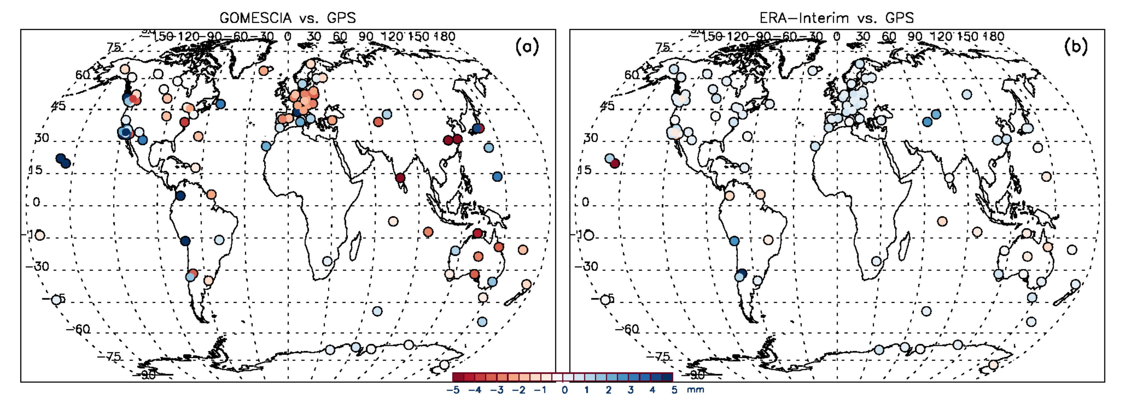
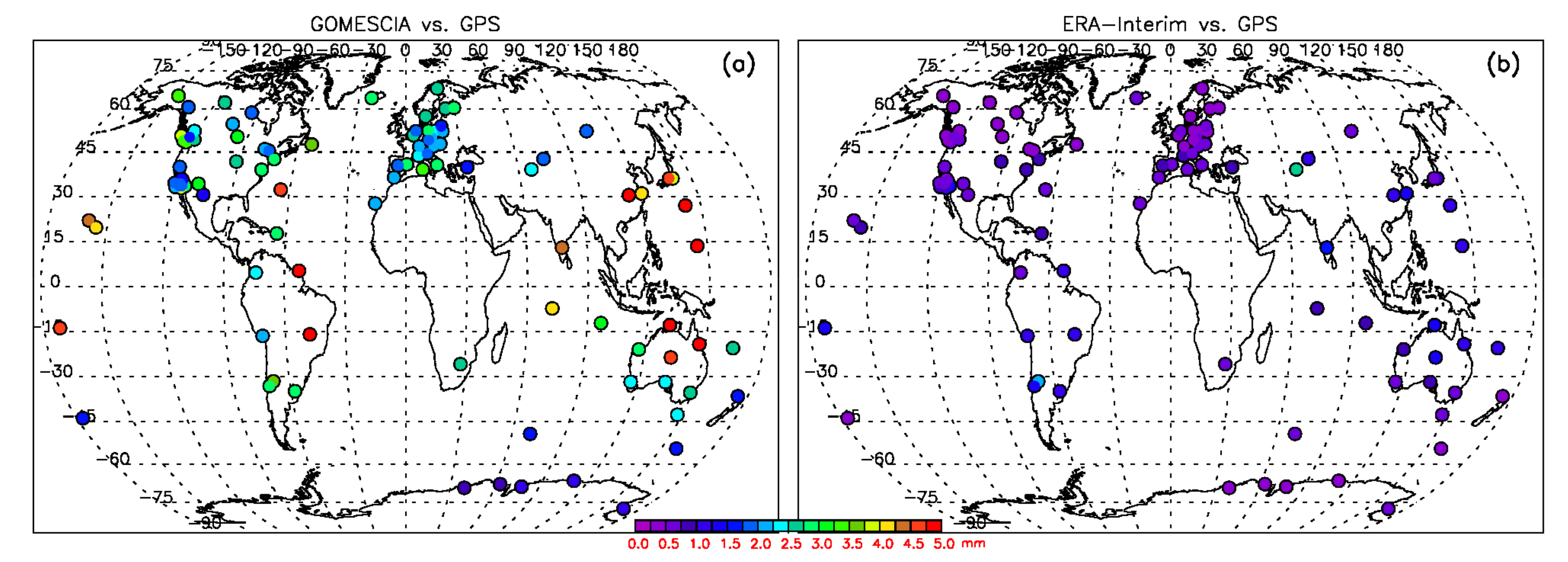
3.1. Dataset Comparison

Before analyzing the spatial and temporal IWV variability of the different datasets, a comparison of the monthly means of those datasets was carried out. Only monthly means are compared as the GOMESCIA climate product is only available with this temporal resolution. The GPS-IWV dataset is treated as the reference dataset, not only because of its high reliability, with root-mean-square values of 1–3 mm [6,35], but also due to the spatial coverage being limited to the GPS site locations. Comparisons between GOMESCIA and ERA-Interim IWV at the GPS site locations are provided in the supplementary material (Figures S1–S3).
In Figure 2, the linear Pearson correlation coefficients between GOMESCIA or ERA-Interim IWV vs. GPS IWV are presented. These are defined as the ratio of the covariance between the two IWV datasets with their standard deviations. The correlation coefficients obtained here are high, and statistically significant at significance level 0.01 (99% confidence interval), for all stations. The average R2 between GOMESCIA and GPS IWV is 0.878, and between ERA-Interim and GPS IWV it is 0.985. The high correlation between ERA-Interim and GPS IWV data has already been noted by Chen and Liu [18], who observed even higher ERA-Interim-radiosonde IWV correlation coefficients. Both GOMESCIA and ERA-Interim agree less well with GPS IWV for island and coastal stations where the resolution of the 1° × 1° GOMESCIA ground pixel and the four surrounding ERA-Interim model (0.75° × 075°) grid limits the accuracy of the IWV field at the exact GPS location [36]. The overall better agreement between GPS and ERA-Interim IWV can probably be explained by the fact that the GPS location and model points are more spatially collocated.
For 60% of the sites, GOMESCIA is dryer than GPS (Figure 3 and Figure S5). This well-known GOMESCIA dry bias can be explained by selecting only cloud-free measurements for the IWV retrieval [11,33]. Conversely, ERA-Interim is slightly wetter than GPS at 70% of sites. The ERA-Interim moist bias of ~0.5 mm occurs particularly in the extra-tropics, with a slight dry bias with respect to GPS in the tropics which has been observed in a number of previous studies [12,36]. Compared to the arithmetic IWV means of the three datasets, GPS has about half of the sites with a positive bias, and half with a negative bias. GOMESCIA has a majority of the sites (63%) negatively biased, whereas ERA-Interim has a majority of the sites (68%) positively biased. The largest mean ERA-Interim or GOMESCIA IWV differences with GPS are found at stations located in coastal regions and regions of complex topography, where representativeness errors limit the comparison of a gridded reanalysis dataset and GPS point observations [12,36]. Representativeness differences between GOMESCIA and GPS IWV measurements at the site locations can explain the larger amplitudes and spatial variability of the IWV mean differences between these two latter datasets.
Figure 4 shows the standard deviations of the mean differences between GOMESCIA or ERA-Interim and GPS IWV that were presented in Figure 3. Bock and Parracho [36] demonstrated that this variable is a very useful metric for representativeness errors between ERA-Interim and GPS IWV. The average value over all sites is smaller between GPS and ERA-interim (0.8 mm) and larger between GPS and GOMESCIA (2.7 mm). This is caused by the larger spatial area around the GPS site covered by GOMESCIA compared to ERA-Interim, and the resulting larger spatial representativeness errors between GOMESCIA and GPS IWV compared to ERA-Interim and GPS IWV. However, a difference in temporal sampling may also play a minor role here, as the GOMESCIA IWV retrievals are not exactly temporally coincident with the GPS observations at the site locations. As such, diurnal IWV variations [20] and differences in cloud cover at both observation times might contribute to a larger variability of the GPS-GOMESCIA IWV differences, compared to GPS-ERA-Interim. The spatial distribution of the standard deviations of the differences in Figure 4 illustrates a slight latitudinal variation, with the largest values mainly obtained between GOMESCIA vs. GPS IWV at tropical island and coastal locations.
It is important to note that the good agreement between ERA-Interim and GPS IWV is not driven by the use of ERA-Interim as a data source for Ps and Tm to convert GPS ZTD to IWV. We obtain very similar results for the statistical parameters in this section if NCEP/NCAR (see also Appendix A) is used as a data source.

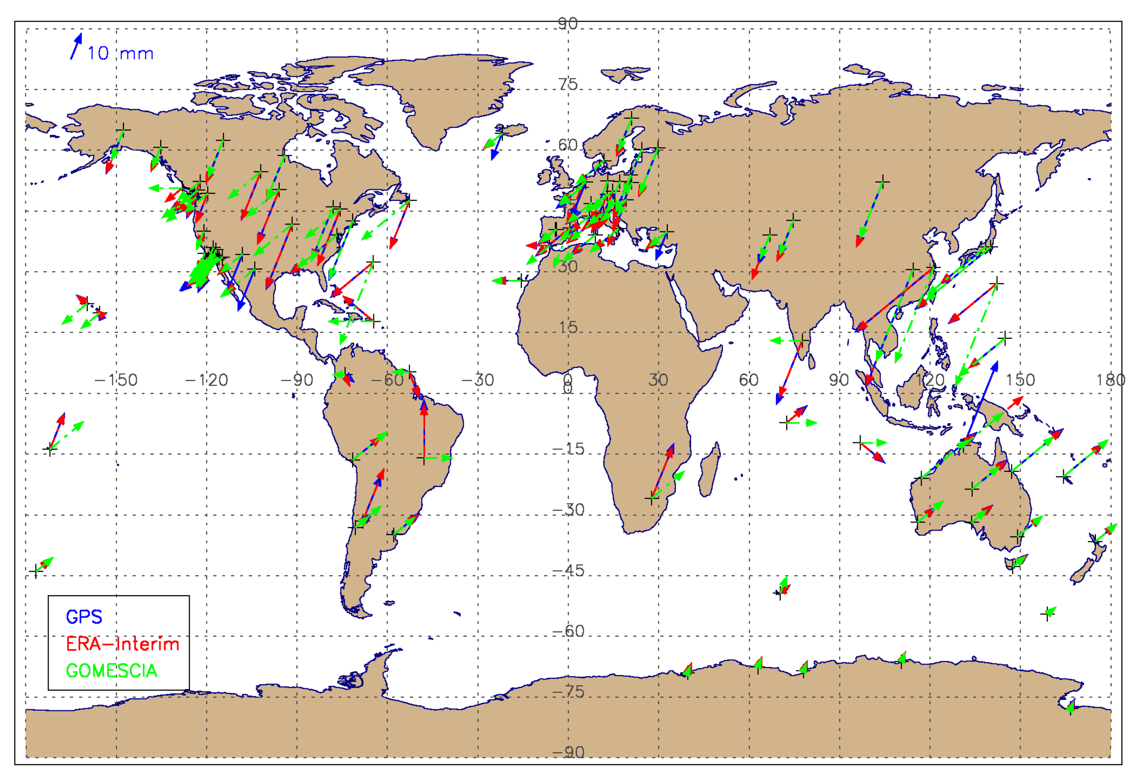
3.2. Seasonal Behavior

To determine the IWV seasonal cycle, we calculate the long-term monthly means of the different datasets using identical time periods for each site. The amplitude is then defined as the difference between the maximum and minimum monthly means and the phase is the month with the maximum IWV monthly mean. The geographical distribution of these parameters for the different datasets are shown in Figure 5. This figure illustrates the seasonal cycle peaking in the summer months for both hemispheres. The amplitude of the seasonal cycle is largest for the Asian Northern Hemisphere sites, where there is a distinct difference between a dry and wet season. In Northern America, the central and eastern sites have larger amplitudes than the western coastal sites. For most of these latter sites, the rainy season is in the winter, when temperatures are low, while the summers are dry but warmer. In Europe, Mediterranean sites have smaller amplitudes and the IWV seasonal cycle peaks one month later compared to the rest of the continent. Overall, there is good consistency among the three datasets, especially between GPS and ERA-Interim. This is also illustrated by histograms of the amplitudes and phases at the sites (Figure 6). These figures also indicate that for about 15 sites in the Northern Hemisphere (mostly US and European), the seasonal cycle peaks one month later in the GOMESCIA dataset with respect to the GPS and ERA-Interim datasets, although the differences between the two monthly means of July and August are less than 1–2 mm. The differences in amplitude are largest in the interval 8–14 mm, which is also the amplitude range for the bulk of the northern hemisphere sites in our sample. However, the correlation between the amplitudes is very good (0.99 between GPS and ERA-Interim, 0.85 between GPS and GOMESCIA).
To conclude, a very similar IWV seasonal cycle for GPS and ERA-Interim was observed with the GOMESCIA seasonal behavior deviating more from the other two datasets, especially at some Northern Hemisphere sites. However, in general, a good agreement in all seasonal cycles was observed.

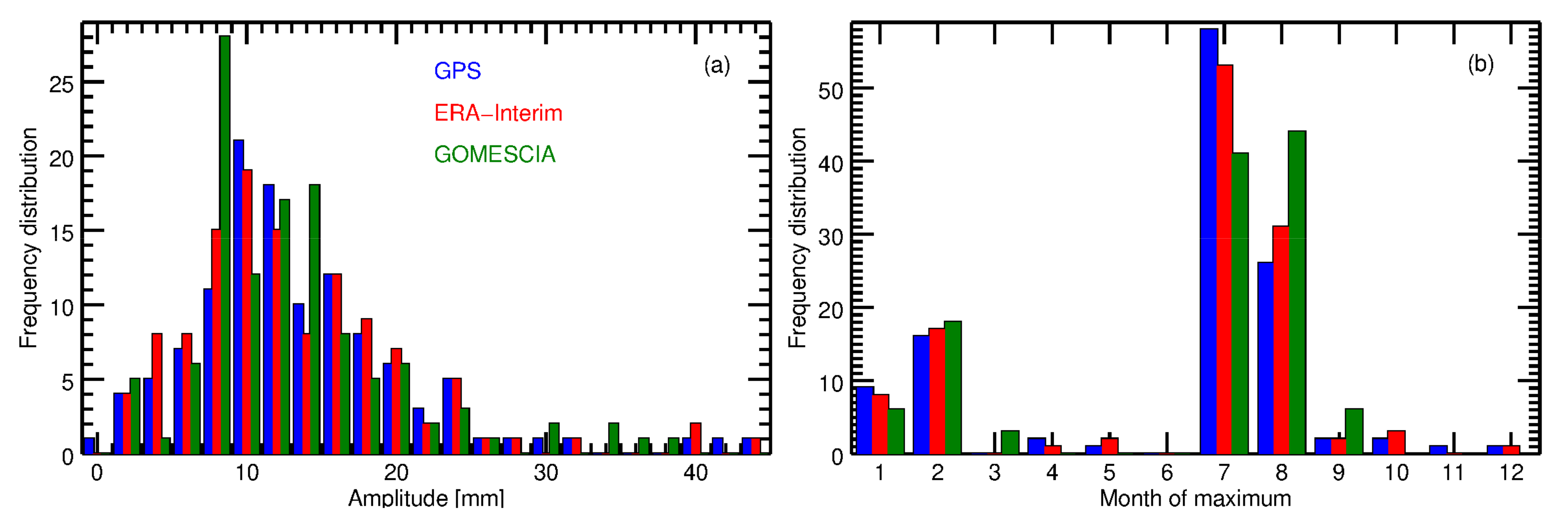
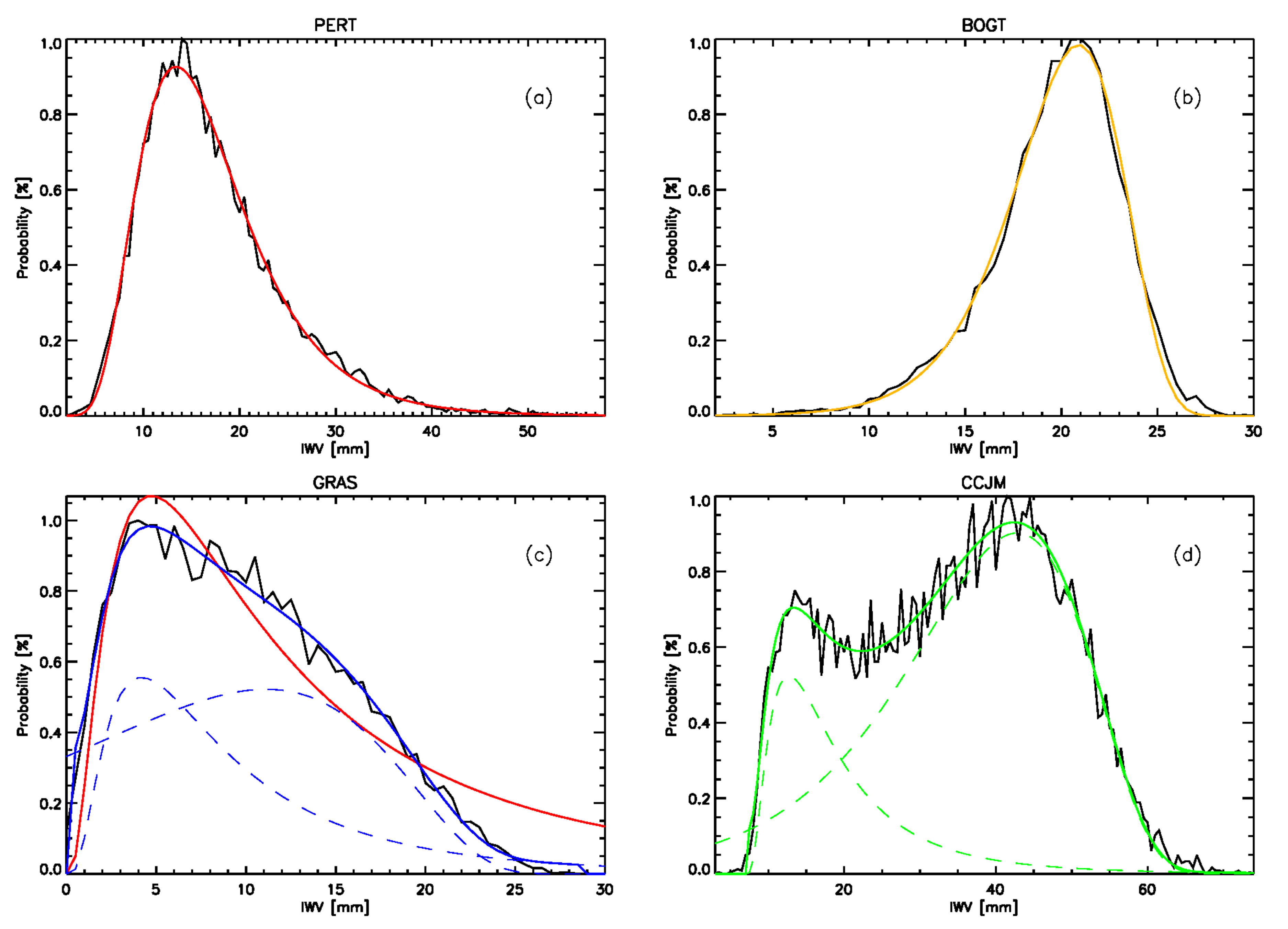
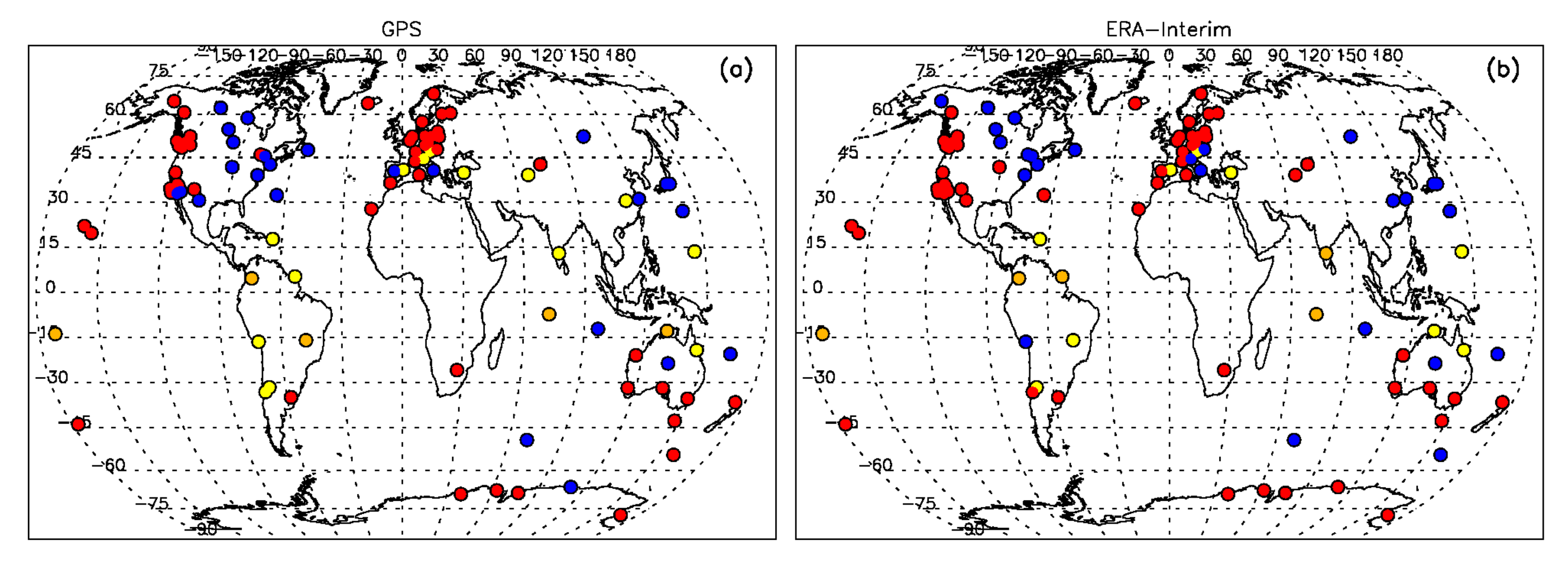
3.3. Frequency Distribution
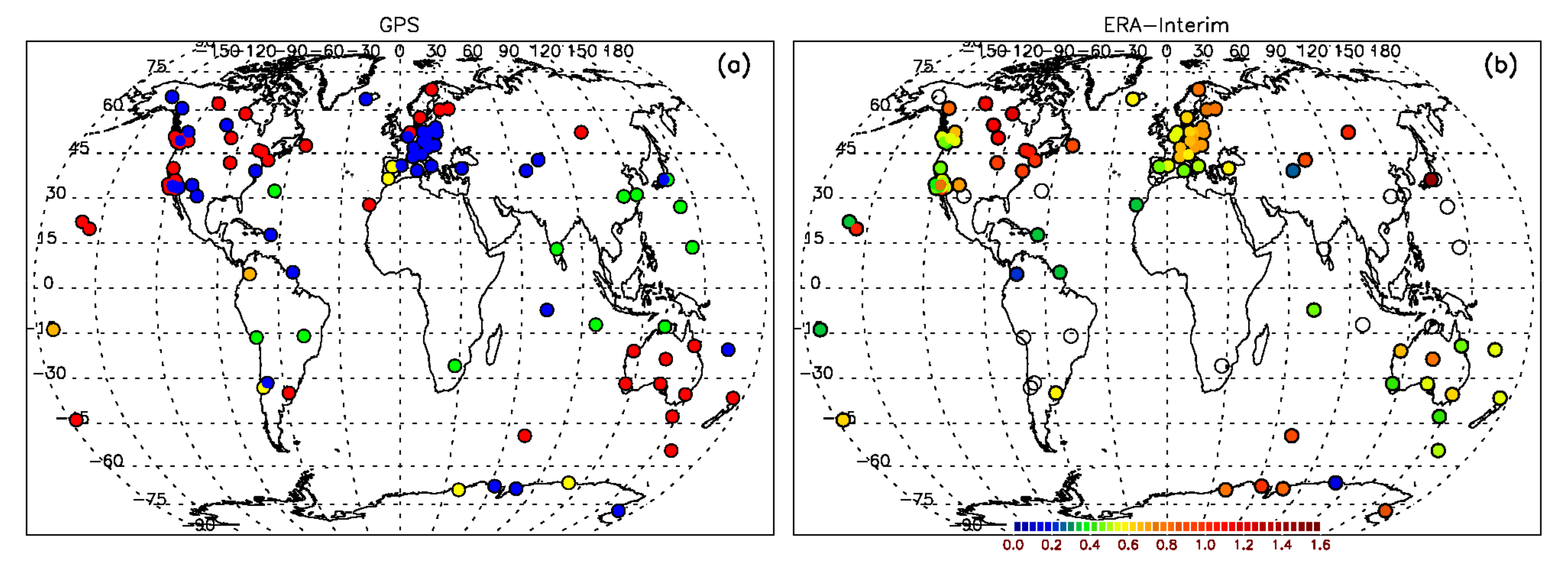
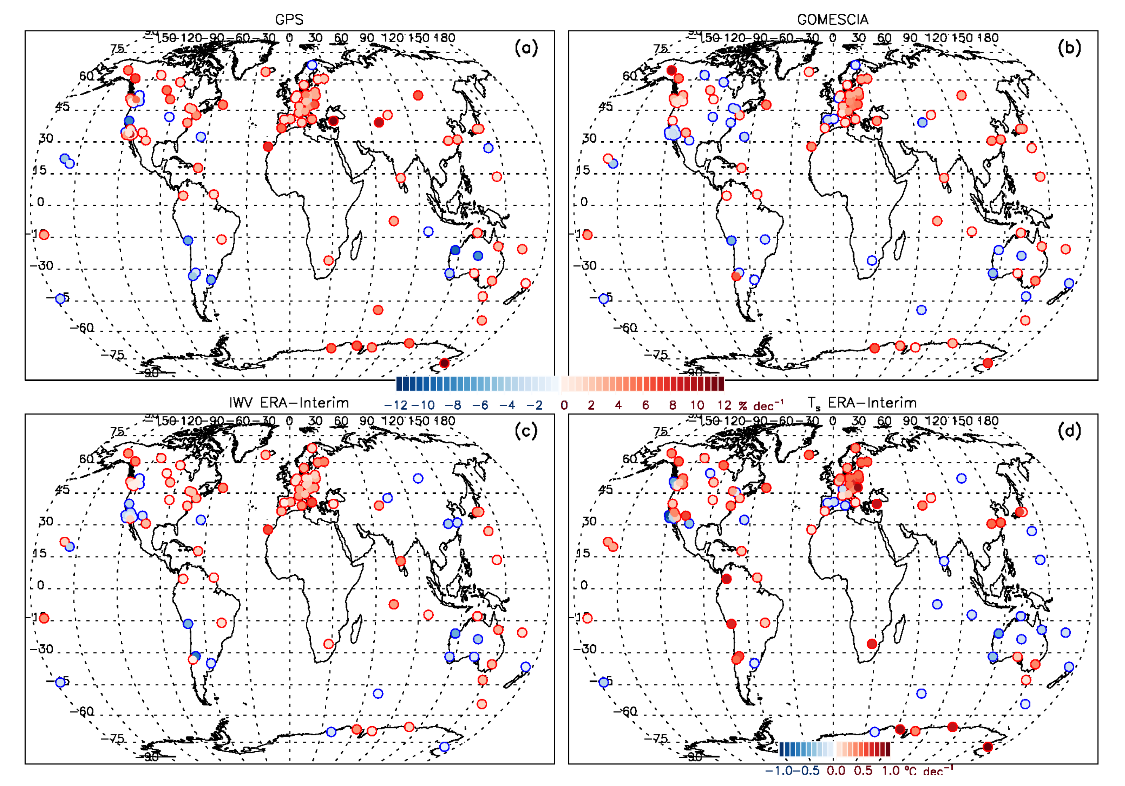
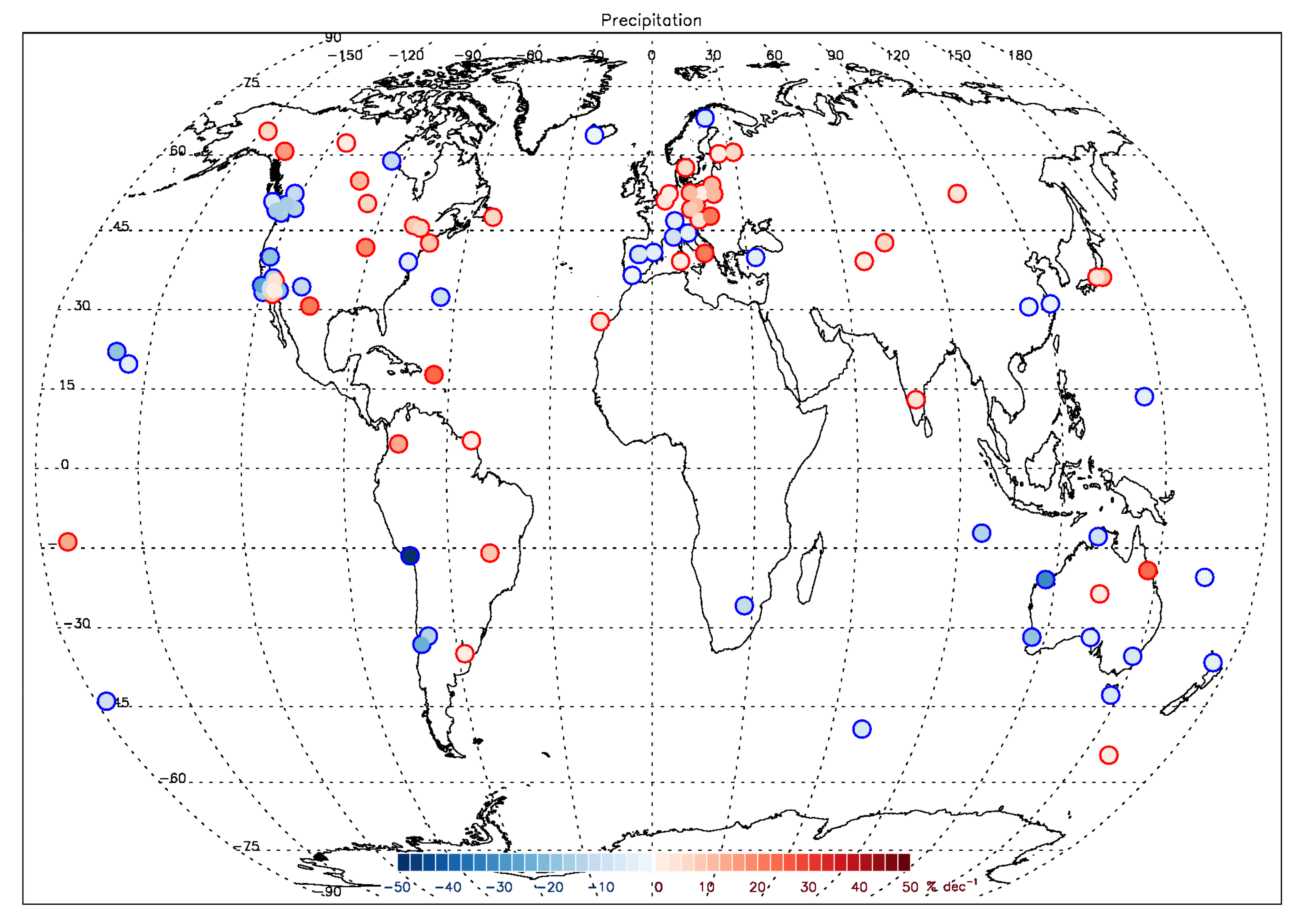
In addition to analyzing seasonal behavior, we may characterize the IWV field properties by the frequency distribution of the IWV data series. This analysis will allow for a classification of geographical regions with similar IWV properties. Unfortunately, we cannot use the GOMESCIA IWV dataset here as this dataset provides only monthly means, undermining the statistical robustness of the observational frequency distribution and its fit by a (log)normal distribution.
From the GPS and ERA-interim IWV time series (available with a 6 h temporal resolution), an IWV frequency distribution was calculated. For each site, a non-linear least squares fit to compute Gaussian, lognormal, and bimodal (two lognormal) distribution functions through those IWV frequency distributions were calculated. For the lognormal distribution function, the same formula as in Foster et al. [14] was adopted and described by three parameters: the median M, the geometric standard deviation (GSD) s, and a threshold parameter t, allowing for a non-zero lower bound (standard lognormal) or even a distribution bounded by an upper value t with the long tail tending towards zero (reverse lognormal). In this latter case (Figure 7b), the upper value t corresponds to the maximum atmospheric moisture capacity in case of complete saturation.
Depending on the values of the chi-square goodness-of-fit statistics (75–80% of the sites) and/or on visual checking of the fitted distribution, the frequency distributions at the sites were categorized into Gaussian, lognormal (standard or reverse), and bimodal distributions. For instance, the distribution function is lognormal if its associated chi-square goodness-of-fit statistic is below a certain threshold value, but bimodal when exceeding this value. Examples of those categories, except the Gaussian, are given in Figure 7a,b,d. These three categories have been identified by Foster et al. [14] in their sample of 10 GPS sites from various climatic regimes around the world.
In addition, an extra category was added between a lognormal and bimodal distribution, defined both visually and by a range of the chi-square goodness-of-fit statistic for the single lognormal distribution fit. For this category, there is one clear lognormal distribution which characterizes the majority of the distribution, and an additional, secondary upper mode lognormal distribution. This second component is required to explain the overall frequency distribution “satisfactorily”, i.e., in terms of the chi-square goodness-of-fit statistic and/or by eye. We call it a “shouldered” lognormal distribution, see Figure 7c. The bulk of the shouldered or bimodal distributions are a combination of a standard lognormal distribution for the lower component, and a reverse lognormal distribution for the upper component, as observed in Figure 7c,d. The upper mode is more ambiguous, due to the overlap between the modes obscuring the telltale asymmetry that would distinguish between them. The origin is related to a large seasonal variation in the median values of IWV, with the dry season characterized by the standard lognormal distribution with a low median, and the wet season characterized by a reverse lognormal distribution with a high median value. This issue will be discussed later in this Section.
Figure 8 displays the geographical distribution of the different categories of the GPS IWV time series. Figure S8a in the supplementary material provides the equivalent results for ERA-Interim. The large majority of the sites have a lognormal IWV distribution, with a few exceptions which have relatively typical Gaussian distributions (e.g., two GPS sites in Antarctica which have very small IWV ranges). It should also be noted that sites with a single reverse lognormal distribution are very uncommon and confined to the tropics: i.e., only for the GPS IWV time series data from BOGT (Bogota, Colombia), SAMO (Samoa Island), and for the ERA-Interim time series at Hawaiian sites and those at DGAR (Diego Garcia Island) and at KOUR (French Guyana), see Figure S8a. Another notable feature is the fact that the occurrence of bimodal distributed IWV time series is almost exclusively restricted to the (sub)tropics or latitudes lower than about 30°. Australia, conversely, is characterized almost uniformly by a standard lognormal distribution. Additionally, northern Europe (Scandinavia) has a standard lognormal IWV distribution, while the rest of Europe (with the exception of some Mediterranean sites which are Gaussian) has shouldered lognormal distributions.
North America is a mix of standard lognormal and shouldered lognormal IWV distributions. The geographical distinction in this continent is further illustrated when considering the GSD values obtained when fitting one single lognormal distribution through the IWV frequency distributions (Figure 8b). The western part of North America is characterized by lower GSD values, while the central and east North American stations have higher GSD values (higher overall histogram width) due to a long tail for higher IWV values in their respective distribution function. This tail is due to the large difference in median values between the (dominant) lower and (weak, if present at all) upper mode of their distributions.
The standard lognormal distributions for the Australian IWV time series, see, e.g., PERT in Figure 7a, are also described by low GSD values, see again Figure 8b and Figure S8b, with the overall histogram width being even lower than those of the North American west coast. In Europe, there appears to be a small increase in the histogram GSDs from west (maritime) to east (continental), although this may be confused with or intermingled with a latitudinal gradient in the GSD. Regardless, western European sites have frequency distributions with a broad peak (i.e., on some occasions the two modes are so close together the overall distribution appears to have a Gaussian distribution, see, e.g., GRAS in Figure 7c), with more distinct modes in the east of Europe (e.g., with a more pronounced tail). The Scandinavian sites have narrower IWV distributions around their peak, but are also strongly (positively) skewed, which explains the large GSDs.
To understand the spatial distribution of the frequency distribution and the impact of the seasonal variability on the shape of the frequency distributions of the GPS and ERA-Interim time series, the seasonal cycle must be removed, as described in Section 3.2. Thereafter, the frequency distribution may be fit again by the same methodology as outlined above. Figure 9 presents the classification of the frequency distributions of those de-seasonalized time series, both for GPS and ERA-Interim locations. In this data it is important to note that no more bimodal distributions remain, and they have become (mostly) single lognormal or even Gaussian distributions. It is now clear that the dominance of the original bimodal distribution for the Asian sites (Figure 8a), is linked to the seasonal monsoonal behavior, which is responsible for the reverse lognormal distribution with high median value (the upper mode), with the lower mode being caused by the corresponding dry season. The bimodality of the (sub)tropical sites is also caused by seasonal IWV variation, and the reverse lognormal distribution is very prominent for the de-seasonalized IWV time series of (sub)tropical coastal or island sites (Figure 9).
Another striking difference between the classification of the frequency distributions from the original and de-seasonalized time series is observed in Europe: after removing the seasonal cycle, the dominating shouldered lognormal distributions in Figure 8a and Figure S8a for GPS and ERA-Interim IWV, respectively, are turned into standard lognormal distributions in Figure 9a,b, respectively. As such, in Europe, it may be assumed the shouldered lognormal distribution originates from seasonal IWV variation.
A remarkable feature of the North American distribution is the very similar geographical distinction in the continent in terms of the GSD values in Figure 8b and the classes of frequency distributions of the de-seasonalized IWV times series, see Figure 9. Sites in western North America (low GSD values) have standard lognormal distributions, the central and east North American stations (higher GSD values) are best fitted by shouldered lognormal distributions. For those latter stations, the IWV variability caused by weather patterns or inter-annual variability appears to be more complex (multimodal) than if the seasonal variability is added.
To conclude, we confirm (for a much larger sample size) the conclusions by Foster et al. [14] that IWV follows a lognormal distribution. This is particularly evident when considering de-seasonalized time series, although Gaussian distributions are then also more common. The seasonal variability in the subtropics and at European sites complicates the frequency distributions, favoring a multimodal (bimodal or shouldered lognormal) description. The opposite is typically true for central and eastern North American sites. Australian sites closely approximate a standard lognormal distribution, with or without considering seasonality. The analysis of the IWV frequency distributions also aids in clustering sites with similar distributions in specific geographical regions or climate regimes. As an example, in North America significant differences in the distributions and their characteristics between the central and eastern sites and the western coastal sites may be observed. This was also the case for this region in terms of the IWV seasonal cycle.

3.4. Linear Trends

In this Section, linear trends were calculated from the different IWV time series data. Two important considerations should be stated, however. Firstly, if we assume the GPS IWV trend magnitude of 0.26 mm decade−1 determined by Wang et al. [20] for the period 1995–2011, and we take into account the effect of auto-correlation and variability [37] from our IWV monthly anomaly time series, we find that, on average, 38 years of monthly data are needed to detect this trend at a 95% confidence level with a probability of 0.90. As we only have 15 years available for most of the stations, we therefore cannot draw firm conclusions on the presence or magnitude of any trend in this study. Secondly, it should be noted that large non-linear inter-annual variations such as ENSO and other teleconnection patterns [38] have an impact on the IWV long-term variability, which should therefore not be well represented by a linear trend. However, the focus of this Section is on the comparison of the IWV linear trends between the different datasets. This first order approximation of the long-term variability, even over shorter time periods, will nevertheless enable an evaluation of temporal stability and consistency of the three distinct IWV datasets.
The linear trends were estimated by minimizing the least squares in the monthly anomaly IWV time series. Monthly anomalies were obtained by subtracting the long-term monthly means from the monthly averages. The standard error of the linear regression slope was used as an estimate of the uncertainty of the trend [39]. Additionally, to test the statistical significance of the trend, the Spearman’s test of trend [40] was applied. These trend uncertainty estimations and indication for the statistical significance, do not take into account the effect of auto-correlation and variability as in Weatherhead et al. [37] and therefore represent underestimations.
The linear trends for the different datasets are shown in Figure 10 for the period of January 1996 to December 2010. It can be seen that the overall agreement of the trends is relatively good. Around two-thirds of the GPS sites have positive trends (23 sites with statistically significant positive trends), whereas this is only true for 55% for GOMESCIA IWV time series (9 sites with statistically significant positive trends). For ERA-Interim, this percentage amounts to 60% (12 sites with statistically significant positive trends). In none of the data sets is the number of sites with statistically significant negative trends larger than 5. As such. there is an overall tendency for positive IWV trends, rather than negative trends, resulting in trend magnitudes, averaged over all stations, of 0.18 mm, 0.08 mm, and 0.11 mm decade−1, for GPS, GOMESCIA, and ERA-Interim, respectively. The mean GPS IWV trend magnitude is very close to the 0.26 mm decade−1 GPS IWV trend as observed by Wang et al. [20], based on a similar IGS dataset. The correlation coefficients between the IWV trend values of the different datasets at the different sites are comparable, with values R2 = 0.66, 0.63, and 0.57 between GPS vs. ERA-Interim, ERA-Interim vs. GOMESCIA, and GPS vs. GOMESCIA, respectively. Trend differences are expected between all-sky IWV datasets (GPS and ERA-Interim) and clear-sky datasets (GOMESCIA), see [9] (their Figure 4).
Next, the geographical consistency in the sign and magnitude of the trends between the different datasets (see Figure 10) for different regions in the world was analyzed. For Europe, the different datasets reveal an overall moistening trend, which is a consistent finding from other studies using different IWV datasets and different time periods, e.g., [41,42,43]. Drying trends over Western Australia and moistening trends over the Indian Ocean appear to be consistent features among the three IWV datasets. Additionally, all three datasets do not show a clear geographical pattern of IWV trends for North America, particularly for GOMESCIA (see also Figure S10). Qualitatively, the trend patterns observed in this paper are in good agreement with Wang et al. [20] and Parracho et al. [12], who, for the period 1995–2011, found (i) positive trends along the coast of the Northeast USA and Eurasia as well as the interior of Australia and Europe, (ii) negative trends covering most of the eastern Pacific around the western coasts of the Americas, and (iii) the Atlantic and Indian Oceans dominated by moistening trends.
For the interpretation of those geographical trend patterns, the trends in the ERA-Interim surface temperature at the GPS site locations were also considered (the lower right panel of Figure 10). As per previous studies [2,4,20,22], the IWV inter-annual variability and trends can globally be explained by temperature change under the assumption that the atmospheric relative humidity (RH) is constant, while saturation vapor pressure increases with air temperature. The scaling ratio amounts in this case around 7% K−1 according to the Clausius-Clapeyron relationship. Over Europe and Western Australia, the respective moistening and drying are associated with surface warming and cooling, respectively. However, over North America, the spatial and temporal correlation between IWV and temperature is worse and opposite trends are even found [22]. In this case, the IWV concentration may be governed more by long-range transportation and the specific precipitation history of air masses [44]. In particular, the cooling and drying (or little change in IWV) for some North American sites close to the Pacific coast (Figure 10 and Figure S10) are associated with a phase change of the Inter-decadal Pacific Oscillation (IPO) from the 1977 to 1998 warm period (peaking at ~1993) to a cold phase around 2012. Surface type and water availability have a strong influence on the evaporation rate and pattern too, in that surface warming may lead to lower RH (as observed over the Southwest USA by Wang et al. [20]), as surface evaporation cannot match the atmospheric demand for moisture, and the Clausius-Clapeyron relation is not valid. Finally, it is important to note that amplitude and correlation between IWV and temperature is also dependent on observation time [20] and season [45].
Finally, trends in precipitation at the site locations were also calculated, as shown in Figure 11. The precipitation data were sampled to the sites from a monthly gridded precipitation dataset [46]. This dataset originates from National Meteorological and Hydrological Services and other external agents and is produced using angular-distance weighting interpolation from the monthly observational data. The spatial pattern of the sign of the precipitation trends overall follows the IWV and surface temperature trend signs, i.e., negative trends in Western Australia and the Pacific coasts of the Americas, and positive trends over continental Europe. The considered time series of surface temperature, IWV, and precipitation therefore seem spatially and temporally correlated with each other, as already highlighted in different studies, e.g., [2,47]. Although water vapor increases globally at a rate close to 7% K−1 with surface warming (as per Clausius-Clapeyron), precipitation increases only with 1 to 3% K−1 [1,48,49,50] according to energetic constraints [50]. Regional moisture divergence/convergence and dynamics also affect the precipitation–temperature–water vapor linkage.
To summarize, the analysis of trends in this paper were over too limited of a time period to evaluate climate change due to the auto-correlation of the time series; nevertheless, the comparisons in this paper demonstrate that considering three independent IWV datasets may provide a spatially and temporally consistent picture when comparing against trends in surface temperature and precipitation.

4. Discussion

Using a sample of 118 globally distributed sites, we analyzed IWV obtained from GPS, GOMESCIA, and ERA-Interim reanalysis for the period 1996–2010. An assessment of the spatiotemporal variability of IWV using these three global, completely distinct, datasets has not been undertaken previously.
For comparison of the different IWV datasets, GPS IWV was chosen as the reference dataset. We found that the ERA-Interim monthly mean IWVs agree better with GPS IWV (the average is equal to 0.985) than GOMESCIA (R2 of 0.878), with correlations at all sites being statistically significant. The lowest correlations are obtained for island and coastal sites where the spatial (horizontal) representation of the IWV field at the site location by the GOMESCIA ground pixel (320 km east–west) and surrounding ERA-interim model grids (80 km) is highly problematic for direct comparison. For 60% of stations the GOMESCIA IWV was found to have a negative (dry) bias compared to GPS IWV, most likely due to the selection of cloud-free observations for the GOMESCIA IWV retrieval. ERA-Interim IWV has a small positive (moist) bias of 0.5 mm compared to GPS IWV for about 70% of the stations, mostly in the extra-tropics, and a slight dry bias in the tropics when compared to GPS. The standard deviation is, on average, smaller between GPS and ERA-interim (0.8 mm) than between GPS and GOMESCIA (2.7 mm). The three datasets also agree very well in terms of the seasonal behavior, with GOMESCIA deviating more from the other two, especially for some Northern Hemisphere sites.
Similar to Foster et al. [14], frequency distributions of the IWV time series are best fitted with lognormal distributions. For subtropical sites and sites in East Asia, two distinct lognormal distributions are however required, where strong seasonality related to the monsoon prescribes a bimodal lognormal density distribution. Sites in Europe and around half of all North American sites have histograms that are best represented by a leading lognormal distribution for the lower component (dry season), added with another, reverse lognormal distribution for the upper component (wet season). These two components can consequently be explained by seasonal IWV behavior. Australia, however, is characterized almost uniformly by a standard lognormal IWV distribution. The distribution of the geometric standard deviations of the lognormal distributions is also geographically very consistent. The analysis of the IWV frequency distributions hence aids in clustering sites with similar distributions in specific geographical regions or climate regimes. For example, in North America, the distributions and their characteristics between the central and eastern sites and the western coastal sites are clearly different. We also found that the central and eastern sites have a IWV seasonal cycle with larger amplitudes than the western coastal sites.
According to the Weatherhead et al. [37] the length of the time series is, in combination with the auto-correlation and variability of the IWV monthly anomalies, too short (38 years are required) to detect the quoted trend of 0.26 mm decade−1 by Wang et al. [20]. If we however concentrate on the geographical consistency of the sign of the linear trends among the different datasets, then we can conclude that IWV is increasing over Europe and the Indian Ocean, while there is a drying trend over Western Australia. The IWV trend sign pattern above North America is less consistent, especially for the GOMESCIA retrieval. Remaining inhomogeneities in the datasets (e.g., due to instrument changes at some GPS sites, changes in the data assimilation sources in ERA-Interim, and when combining the measurements of the individual instruments to build up the GOMESCIA time series) might impact the results. However, this study highlights that combining information from three distinct IWV datasets enables the consistent characterization of IWV variability and its relationship with surface temperature and precipitation. For instance, over Europe and Western Australia, the respective moistening and drying are associated with surface warming and cooling, respectively. Moreover, the spatial pattern of the sign of the precipitation trends in those regions follows these IWV and surface temperature trend signs with positive trends over continental Europe and negative trends in Western Australia.
For future studies, the homogenization of the IGS GPS dataset will further improve its reliability for long-term variability assessments. Van Malderen et al. [29] compared different statistical break-point detection methods on synthetic IWV differences between IGS GPS and ERA-Interim at our sample sites, and identified a number of promising methods which could be applied to real-world GPS datasets, preferentially in combination with metadata on site instrument changes. In addition, the next homogeneous reprocessing of the IGS tropospheric product will extend this dataset further. Finally, the most recent state-of-the-art reanalysis dataset of ECMWF, ERA5 [51], has improved temporal (1 h) and spatial resolution (horizontal resolution of 31 km, 137 vertical levels to 1 hPa) compared to ERA-Interim, and has an upgraded assimilation method.

Supplementary Materials

The following are available online at https://www.mdpi.com/article/10.3390/rs14041050/s1, Figure S1: Correlation coefficients between GOMESCIA and ERA-Interim; Figure S2: Mean differences between GOMESCIA and ERA-Interim; Figure S3: Standard deviations between GOMESCIA and ERA-Interim; Figure S4: Correlation coefficients over Northern America and Europa; Figure S5: Mean differences over Northern America and Europa; Figure S6: Standard deviations over Northern America and Europa; Figure S7: Seasonal cycle over Northern America and Europa; Figure S8: Similar to Figure 8, but mirrored between GPS and ERA-Interim; Figure S9: GSD distribution over Northern America and Europe; Figure S10: IWV and surface temperature trends over Northern America and Europe; Table S1: List of IGS stations.

Author Contributions

Conceptualization, R.V.M. and E.P.; methodology, R.V.M. and E.P.; validation, R.V.M., E.P. and S.B.; formal analysis, R.V.M.; investigation, R.V.M., E.P. and G.S.; data curation, R.V.M., E.P. and S.B.; writing—original draft preparation, R.V.M.; writing—review and editing, R.V.M., E.P., G.S., S.B., T.W., H.B., C.B. and J.J.; visualization, R.V.M.; supervision, C.B.; funding acquisition, C.B. All authors have read and agreed to the published version of the manuscript.

Funding

The research has been undertaken in the framework of the Solar-Terrestrial Centre of Excellence (STCE), funded by the Belgian Federal Science Policy Office. R.V.M., E.P. and H.B. are members of the Solar-Terrestrial Centre of Excellence.

Institutional Review Board Statement

Not applicable.

Informed Consent Statement

Not applicable.

Data Availability Statement

Publicly available datasets were analyzed in this study. The IGS repro 1 data can be found at https://igs.org/acc/reprocessing (last access on 21 December 2021), the ERA-Interim data at https://www.ecmwf.int/en/forecasts/datasets/reanalysis-datasets/era-interim (accessed on 21 December 2021), and the NCEP/NCAR reanalysis at https://psl.noaa.gov/data/gridded/data.ncep.reanalysis.html (accessed on 21 December 2021). The GOMESCIA data presented in this study are openly available in WDCC doi:10.1594/WDCC/GOME-EVL_water_vapor_clim_v2.2 [52] and the precipitation data in CEDA at doi:10.5285/58a8802721c94c66ae45c3baa4d814d0 [46].

Acknowledgments

This work has been presented at various workshops organized within the framework of the European COST Action ES1206 GNSS4SWEC (GNSS for Severe Weather and Climate monitoring; http://www.cost.eu/COST_Actions/essem/ES1206, accessed on 21 December 2021), so we are indebted to many colleagues contributing with their feedback and discussions!

Conflicts of Interest

The authors declare no conflict of interest.

Appendix A

The formulas used for the GPS ZTD to IWV conversion [11] contain two meteorological variables: the surface pressure and the weighted mean temperature. Of these two, the impact of the surface pressure on the IWV is largest: a 1 hPa change in Ps gives an IWV change of 0.36 mm, whereas a 1 K change in Tm leads to an IWV change in the range 0.05 to 0.20 mm, depending on the ZTD and Ps values. If the Bevis et al. [24] linear Tm−Ts regression is used (Tm = 70.2 + 0.72 Ts), a 1 °C change in Ts brings an IWV change of 0.03 to 0.15 mm, as the Tm changes with 0.72 K for a 1 °C Ts change. It should, however, be noted that the surface temperature also appears in the formula to convert the surface pressure from the height of its data source to the GPS station’s height. Parracho [31] showed that the Ps error associated for Ts varying from 278 to 298 K can amount up to ±2 hPa, when extrapolating pressure measurements within the first 500m with their used equation. Further reading on the quantification of the sensitivity of IWV error to errors in the independent parameters is available in Parracho [31] as well.
Different data sources, either observational or reanalysis datasets, exist for the surface pressure and temperature and weighted mean temperature. To assess the impact those different data sources might have on the retrieved IWV values and trends, we analyzed the comparison between two IWV datasets with different sources for these parameters. Hence, the results shown here are specific to those datasets. The different surface data sources used here are the World Meteorological Organization network of meteorological SYNOP (synoptic) weather stations—only available for about 40 IGS stations of our sample—and the ERA-Interim and National Centers for Environmental Prediction/National Center for Atmospheric Research NCEP/NCAR Reanalysis 1 datasets [53]. Compared to ERA-Interim, NCEP/NCAR has a coarser spatial resolution (2.5° × 2.5°, or about 210 km) and only 17 vertical levels but is also available four times daily. The data assimilation (3D-Var) and the global spectral model are identical to the global system implemented operationally at NCEP in January 1995, but with a higher horizontal resolution. The assimilation database has been enhanced with many observations not available in real time for operational use at that time. We applied exactly the same methodology as for ERA-Interim to retrieve the IWV and auxiliary meteorological values from NCEP/NCAR at the GPS station locations and heights.
The weighted mean temperature is either obtained from the surface temperature by the Bevis et al., regression, or calculated from the vertical profile data supplied by the reanalysis datasets. In Table A1, we present the means—weighted by the number of observations for each station—of (from left to right) the IWV differences, the absolute value of the IWV differences, the standard deviation of the IWV differences, the linear correlation coefficients between the IWVs, the IWV trend differences, and finally the absolute IWV trend differences between two GPS IWV datasets that disagree only by one or more of these auxiliary meteorological parameters. The differences and correlations are calculated between all available, coincident measurements (at 0, 6, 12, 18 h) at the different sites, while the trends are calculated from the monthly anomalies. Table A1 confirms the larger impact of the surface pressure than the surface temperature and weighted mean temperature on the IWV differences, but also on the derived IWV trends (largest values are obtained for case (b)). Moreover, the slope of the linear regression (with a correlation coefficient of 0.84) between the Ps and IWV differences (i.e., the individual values of the first column of case (b), not the mean) between the different corresponding datasets for the 40 IGS stations is equal to the −0.34, which is very close to the mentioned (theoretical) IWV change of 0.36 mm per 1 hPa surface pressure change, confirming the acceptable data quality of the pressure observations at the selected meteorological weather stations close to an IGS station. Although large differences exist between the surface and mean temperatures taken from the synoptic observations or ERA-Interim, see cases (c) and (d) in Table A2, the resulting IWV mean differences remain very small, as well as the IWV trend differences (the corresponding cases (c) and (d) in Table A1). The values for (d) can be compared to the study undertaken by Wang et al. [20]. For our sample of data, the slopes of the linear regression between the Ts and Tm mean differences with the IWV differences (i.e., the individual values of the first columns in respectively cases (c) and (d), respectively) of these datasets are 0.03 and 0.05, respectively (with correlation coefficients equal to 0.90 and 0.66, respectively), which are the lower end values of the derived ranges in the previous paragraph.
The effect of the used reanalysis dataset (see case (f) in Table A1) on the resulting IWV mean differences and trends are comparable with the numbers for the effects of the temperatures (cases (c) to (e) in Table A1), except for the absolute mean difference. Apparently, the larger mean differences between the surface pressures of the two reanalyses (case (a) Table A2), compared to the pressure differences between ERA-Interim and SYNOP (case (b) in Table A2), are partially compensated by the differences in mean temperatures between the two reanalyses (case (e) in Table A2). The same argument can be used to explain the smaller differences in IWV mean differences and trends between datasets generated completely with SYNOP observations and ERA-Interim on one hand (case (g) in Table A1), compared to changing only the source data of the surface pressure (case (b) in Table A1). Finally, we note that the largest IWV mean differences are obtained when comparing the ERA-Interim IWVs with the IWVs retrieved from the IGS ZTDs (see case (a) in Table A1, which is comparable to the analysis in Section 3.1 for ERA-Interim and IGS). This follows from the fact that these two are the most independent IWV datasets shown in the table. It also illustrates the added value (negative or positive, this has been investigated in the paper) of the IGS data to the reanalysis data. The largest IWV trend differences are obtained for the cases (a), (b), and (g) in Table A1, implying that the IWV trends are driven by the trends in the surface pressures and the trends present in the ZTD time series themselves. The impact of the trends in the temperatures seems from the point of view of this analysis (relying on the weighted means of the entire set of stations) less determinative for the IWV trends. In any case, a correlation between the IWV trend differences and trend differences in Ps, Ts, and Tm cannot be found, as was the case for the IWV mean differences.
Table A1. Weighted mean values (and their corresponding standard deviations) of the statistical parameters describing differences computed between two different IWV datasets (from left to right: mean differences, mean absolute difference, standard deviation (SD) of difference, mean trend difference, mean absolute trend difference), demonstrating the impact of different variables or dataset choices. ERA stands for ERA-Interim, NCEP for NCEP/NCAR, Bevis denotes if the Bevis et al. [24] Tm−Ts regression is used. An asterisk * denotes that the comparison was done for only 40 stations, i.e., those stations with a synoptic (SYNOP) station within 30 km distance.
Mean Difference (mm)Mean Abs. Difference (mm)SD (mm)Trend (mm dec−1)Abs Trend (mm dec−1)
(a)Tm = ERA, Ps = ERA: influence IGS data
IWV = ERA−0.313 ± 1.0110.669 ± 0.8183.8070.962−0.102 ± 0.4570.322 ± 0.338
(b)Tm = ERA, Ps = ERA: influence Ps
Tm = ERA, and Ps =SYNOP *−0.200 ± 0.614 0.301 ± 0.570 7.575 0.961 −0.290 ± 0.7520.353 ± 0.724
(c)Tm = Bevis and Ts = ERA, Ps = SYNOP: influence Ts
Tm = Bevis and Ts = SYNOP, Ps = SYNOP *0.009 ± 0.0250.020 ± 0.0170.0291.0000.013 ± 0.244 -0.107 ± 0.219
(d)Tm = ERA, Ps = ERA: influence Bevis et al., regression (Tm)
Tm = Bevis and Ts = ERA, Ps = ERA0.044 ± 0.0920.069 ± 0.0750.025 1.000 −0.004 ± 0.031 -0.018 ± 0.025
(e)Tm = ERA, Ps = SYNOP: influence Ts and Bevis et al., regression
Tm = Bevis and Ts = SYNOP, Ps = SYNOP *0.026 ± 0.0710.051 ± 0.0550.0521.0000.001 ± 0.2480.110 ± 0.221
(f)Tm = ERA, Ps = ERA: influence reanalysis dataset
Tm = NCEP, and Ps = NCEP−0.034 ± 0.2860.168 ± 0.2330.1540.995−0.015 ± 0.1440.083 ± 0.118
(g)Tm = ERA, Ps = ERA: observational vs. reanalysis dataset
Tm = Bevis and Ts = SYNOP, Ps = SYNOP *−0.073 ± 0.4030.223 ± 0.3424.7050.971−0.210 ± 0.6670.259 ± 0.649
Table A2. Weighted mean values (and their corresponding standard deviations) of the same statistical parameters as in Table A1 describing differences between Ps (cases (a) and (b), in hPa) and Tm (cases (c), (d), and (e), in K) taken from different data sources ((a), (b), (c), and (e)) or computed by a different method (d). The cases (b), (c), and (d) correspond to the cases in Table A1.
Mean Difference (hPa or K)Mean Abs. Difference (hPa or K)SD (hPa or K)Trend (hPa dec−1 or K dec−1)Abs Trend (hPa dec−1 or K dec−1)
(a)Ps = ERA
Ps =NCEP−0.179 ± 0.7880.447 ± 0.6731.2410.9740.083 ± 0.3890.214 ± 0.335
(b)Ps = ERA
Ps =SYNOP *0.031 ± 0.6110.357 ± 0.4940.7860.9890.052 ± 0.4010.277 ± 0.292
(c)Tm = Bevis and Ts = ERA
Tm = Bevis and Ts = SYNOP *0.267 ± 0.6220.503 ± 0.4472.8780.9790.197 ± 0.8790.502 ± 0.744
(d)Tm = ERA
Tm = Bevis and Ts = ERA0.508 ± 1.5831.235 ± 1.1088.0990.8040.101 ± 0.2130.188 ± 0.140
(e)Tm = ERA
Tm = NCEP−1.236 ± 0.6451.280 ± 0.5528.6780.9260.080 ± 0.2570.169 ± 0.209

References

  1. Held, I.M.; Soden, B.J. Robust Responses of the Hydrological Cycle to Global Warming. J. Clim. 2006, 19, 5686–5699. [Google Scholar] [CrossRef]
  2. Trenberth, K.E.; Fasullo, J.; Smith, L. Trends and variability in column-integrated atmospheric water vapor. Clim. Dyn. 2005, 24, 741–758. [Google Scholar] [CrossRef]
  3. Wentz, F.J.; Ricciardulli, L.; Hilburn, K.; Mears, C. How much more rain will global.warming bring? Science 2007, 317, 233–235. [Google Scholar] [CrossRef]
  4. Mears, C.A.; Santer, B.D.; Wentz, F.J.; Taylor, K.E.; Wehner, M.F. Relationship between temperature and precipitable water changes over tropical oceans. Geophys. Res. Lett. 2007, 34, L24709. [Google Scholar] [CrossRef] [Green Version]
  5. Kampfer, N. Monitoring Atmospheric Water Vapour: Ground-Based Remote Sensing and In-Situ Methods; Springer Science: Berlin/Heidelberg, Germany, 2013. [Google Scholar] [CrossRef]
  6. Guerova, G.; Jones, J.; Douša, J.; Dick, G.; de Haan, S.; Pottiaux, E.; Bock, O.; Pacione, R.; Elgered, G.; Vedel, H.; et al. Review of the state of the art and future prospects of the ground-based GNSS meteorology in Europe. Atmos. Meas. Tech. 2016, 9, 5385–5406. [Google Scholar] [CrossRef] [Green Version]
  7. Morland, J.; Collaud Coen, M.; Hocke, K.; Jeannet, P.; Mätzler, C. Tropospheric water vapour above Switzerland over the last 12 years. Atmos. Chem. Phys. 2009, 9, 5975–5988. [Google Scholar] [CrossRef] [Green Version]
  8. Hocke, K.; Kämpfer, N.; Gerber, C.; Mätzler, C. A complete long-term series of integrated water vapour from ground-based microwave radiometers. Int. J. Remote Sens. 2011, 32, 751–765. [Google Scholar] [CrossRef]
  9. Schröder, M.; Lockhoff, M.; Fell, F.; Forsythe, J.; Trent, T.; Bennartz, R.; Borbas, E.; Bosilovich, M.G.; Castelli, E.; Hersbach, H.; et al. The GEWEX Water Vapor Assessment archive of water vapour products from satellite observations and reanalyses. Earth Syst. Sci. Data 2018, 10, 1093–1117. [Google Scholar] [CrossRef] [PubMed] [Green Version]
  10. Vaquero-Martinez, J.; Anton, M. Review on the Role of GNSS Meteorology in Monitoring Water Vapor for Atmospheric Physics. Remote Sens. 2021, 13, 2287. [Google Scholar] [CrossRef]
  11. Van Malderen, R.; Brenot, H.; Pottiaux, E.; Beirle, S.; Hermans, C.; De Mazière, M.; Wagner, T.; De Backer, H.; Bruyninx, C. A multi-site intercomparison of integrated water vapour observations for climate change analysis. Atmos. Meas. Tech. 2014, 7, 2487–2512. [Google Scholar] [CrossRef] [Green Version]
  12. Parracho, A.C.; Bock, O.; Bastin, S. Global IWV trends and variability in atmospheric reanalyses and GPS observations. Atmos. Chem. Phys. 2018, 18, 16213–16237. [Google Scholar] [CrossRef] [Green Version]
  13. Zhao, Q.; Yao, Y.; Yao, W. Studies of Precipitable Water Vapour Characteristics on a Global Scale. Int. J. Remote Sens. 2019, 40, 72–88. [Google Scholar] [CrossRef]
  14. Foster, J.; Bevis, M.; Raymond, W. Precipitable water and the lognormal distribution. J. Geophys. Res. 2006, 111, D15102. [Google Scholar] [CrossRef] [Green Version]
  15. Sherwood, S.C.; Roca, R.; Weckwerth, T.M.; Andronova, N.G. Tropospheric water vapor, convection, and climate. Rev. Geophys. 2010, 48, RG2001. [Google Scholar] [CrossRef] [Green Version]
  16. Bock, O.; Willis, P.; Wang, J.; Mears, C. A high-quality, homogenized, global, long-term (1993–2008) DORIS precipitable water data set for climate monitoring and model verification. J. Geophys. Res. Atmos. 2014, 119, 7209–7230. [Google Scholar] [CrossRef]
  17. Mieruch, S.; Schröder, M.; Noël, S.; Schulz, J. Comparison of decadal global water vapor changes derived from independent satellite time series. J. Geophys. Res. Atmos. 2014, 119, 12489–12499. [Google Scholar] [CrossRef]
  18. Chen, B.; Liu, Z. Global water vapor variability and trend from the latest 36 year (1979 to 2014) data of ECMWF and NCEP reanalyses, radiosonde, GPS, and microwave satellite. J. Geophys. Res. Atmos. 2016, 121, 11442–11462. [Google Scholar] [CrossRef]
  19. Schröder, M.; Lockhoff, M.; Forsythe, J.M.; Cronk, H.Q.; Vonder Haar, T.H.; Bennartz, R. The GEWEX Water Vapor Assessment: Results from Intercomparison, Trend, and Homogeneity Analysis of Total Column Water Vapor. J. Appl. Meteorol. Climatol. 2016, 55, 1633–1649. [Google Scholar] [CrossRef]
  20. Wang, J.; Dai, A.; Mears, C. Global Water Vapour Trend from 1988 to 2011 and Its Diurnal Asymmetry Based on GPS, Radiosonde, and Microwave Satellite Measurements. J. Clim. 2016, 29, 5205–5222. [Google Scholar] [CrossRef]
  21. Mears, C.A.; Smith, D.K.; Ricciardulli, L.; Wang, J.; Huelsing, H.; Wentz, F.J. Construction and Uncertainty Estimation of a Satellite-Derived Total Precipitable Water Data Record Over the World’s Oceans. Earth Space Sci. 2018, 5, 197–210. [Google Scholar] [CrossRef] [Green Version]
  22. Wagner, T.; Beirle, S.; Grzegorski, M.; Platt, U. Global trends (1996–2003) of total column precipitable water observed by Global Ozone Monitoring Experiment (GOME) on ERS-2 and their relation to near-surface temperature. J. Geophys. Res. 2006, 111, D12102. [Google Scholar] [CrossRef] [Green Version]
  23. Dee, D.P.; Uppala, S.M.; Simmons, A.J.; Berrisford, P.; Poli, P.; Kobayashi, S.; Andrae, U.; Balmaseda, M.A.; Balsamo, G.; Bauer, P.; et al. The ERA-Interim reanalysis: Configuration and performance of the data assimilation system. Q. J. R. Meteorol. Soc. 2011, 137, 553–597. [Google Scholar] [CrossRef]
  24. Bevis, M.; Businger, S.; Herring, T.A.; Rocken, C.; Anthes, R.A.; Ware, R.H. GPS meteorology: Remote sensing of atmospheric water vapor using the global positioning system. J. Geophys. Res. 1992, 97, 15787–15801. [Google Scholar] [CrossRef]
  25. Dow, J.M.; Neilan, R.E.; Rizos, C. The International GNSS service in a changing landscape of Global Navigation Satellite Systems. J. Geod. 2009, 83, 191–198. [Google Scholar] [CrossRef]
  26. Byun, S.H.; Bar-Sever, Y.E. A new type of troposphere zenith path delay product of the international GNSS service. J. Geod. 2009, 83, 367–373. [Google Scholar] [CrossRef] [Green Version]
  27. Vey, S.; Dietrich, R.; Fritsche, M.; Rülke, A.; Steigenberger, P.; Rothacher, M. On the homogeneity and interpretation of precipitable water time series derived from global GPS observations. J. Geophys. Res. 2009, 114, D10101. [Google Scholar] [CrossRef] [Green Version]
  28. Ning, T.; Wickert, J.; Deng, Z.; Heise, S.; Dick, G.; Vey, S.; Schöne, T. Homogenized Time Series of the Atmospheric Water Vapor Content Obtained from the GNSS Reprocessed Data. J. Clim. 2016, 29, 2443–2456. [Google Scholar] [CrossRef]
  29. Van Malderen, R.; Pottiaux, E.; Klos, A.; Domonkos, P.; Elias, M.; Ning, T.; Bock, O.; Guijarro, J.; Alshawaf, F.; Hoseini, M.; et al. Homogenizing GPS integrated water vapor time series: Benchmarking break detection methods on synthetic datasets. Earth Space Sci. 2020, 7, e2020EA001121. [Google Scholar] [CrossRef] [Green Version]
  30. Wang, J.; Zhang, L.; Dai, A.; Van Hove, T.; Van Baelen, J. A near-global, 2-hourly data set of atmospheric precipitable water from ground-based GPS measurements. J. Geophys. Res. 2007, 112, D11107. [Google Scholar] [CrossRef] [Green Version]
  31. Parracho, A.C. Study of Trends and Variability of Atmospheric Integrated Water Vapour with Climate MODELS and Observations from Global GNSS Network. Ph.D. Thesis, Université Pierre et Marie Curie, Paris, France, 12 December 2017. Available online: http://www.theses.fr/2017PA066524 (accessed on 21 December 2021).
  32. Deblonde, G.; Macpherson, S.; Mireault, Y.; Heroux, P. Evaluation of GPS precipitable water over Canada and the IGS network. J. Appl. Meteorol. 2005, 44, 153–166. [Google Scholar] [CrossRef]
  33. Beirle, S.; Lampel, J.; Wang, Y.; Mies, K.; Dörner, S.; Grossi, M.; Loyola, D.; Dehn, A.; Danielczok, A.; Schröder, M.; et al. The ESA GOME-Evolution “Climate” water vapor product: A homogenized time series of H2O columns from GOME, SCIAMACHY, and GOME-2. Earth Syst. Sci. Data 2018, 10, 449–468. [Google Scholar] [CrossRef]
  34. Hagemann, S.; Bengtsson, L.; Gendt, G. On the determination of atmospheric water vapor from GPS measurements. J. Geophys. Res. 2003, 108, 4678. [Google Scholar] [CrossRef] [Green Version]
  35. Gui, K.; Che, H.; Chen, Q.; Zeng, Z.; Liu, H.; Wang, Y.; Zheng, Y.; Sun, T.; Liao, T.; Wang, H.; et al. Evaluation of radiosonde, MODIS-NIR-Clear, and AERONET precipitable water vapor using IGS ground-based GPS measurements over China. Atmos. Res. 2017, 197, 461–473. [Google Scholar] [CrossRef]
  36. Bock, O.; Parracho, A.C. Consistency and representativeness of integrated water vapour from ground-based GPS observations and ERA-Interim reanalysis. Atmos. Chem. Phys. 2019, 19, 9453–9468. [Google Scholar] [CrossRef] [Green Version]
  37. Weatherhead, E.C.; Reinsel, G.C.; Tiao, G.C.; Meng, X.-L.; Choi, D.; Cheang, W.-K.; Keller, T.; DeLuisi, J.; Wuebbles, D.J.; Kerr, J.B.; et al. Factors affecting the detection of trends: Statistical considerations and applications to environmental data. J. Geophys. Res. 1998, 103, 17149–17161. [Google Scholar] [CrossRef]
  38. Wagner, T.; Beirle, S.; Dörner, S.; Borger, C.; Van Malderen, R. Identification of atmospheric and oceanic teleconnection patterns in a 20-year global data set of the atmospheric water vapour column measured from satellites in the visible spectral range. Atmos. Chem. Phys. 2021, 21, 5315–5353. [Google Scholar] [CrossRef]
  39. Ross, R.J.; Elliott, W.P. Tropospheric water vapor climatology and trends over North America: 1973–93. J. Clim. 1996, 9, 3561–3574. [Google Scholar] [CrossRef] [Green Version]
  40. Ross, R.J.; Elliott, W.P. Radiosonde-based Northern Hemisphere tropospheric water vapor trends. J. Clim. 2001, 14, 1602–1612. [Google Scholar] [CrossRef]
  41. Alshawaf, F.; Zus, F.; Balidakis, K.; Deng, Z.; Hoseini, M.; Dick, G.; Wickert, J. On the statistical significance of climatic trends estimated from GPS tropospheric time series. J. Geophys. Res. Atmos. 2018, 123, 10967–10990. [Google Scholar] [CrossRef]
  42. Yuan, P.; Hunegnaw, A.; Alshawaf, F.; Awange, J.; Klos, A.; Teferle, F.N.; Kutterer, H. Feasibility of ERA5 integrated water vapor trends for climate change analysis in continental Europe: An evaluation with GPS (1994–2019) by considering statistical significance. Remote Sens. Environ. 2021, 260, 112416. [Google Scholar] [CrossRef]
  43. Yuan, P.; Van Malderen, R.; Yin, X.; Vogelmann, H.; Awange, J.; Heck, B.; Kutterer, H. Characterizations of Europe’s integrated water vapor and assessments of atmospheric reanalyses using more than two decades of ground-based GPS. Atmos. Chem. Phys. Discuss. 2021. [Google Scholar] [CrossRef]
  44. Ross, R.J.; Elliott, W.P.; Seidel, D.J. Lower tropospheric humidity–temperature relationships in radiosonde observations and atmospheric general circulation models. J. Hydrometeorol. 2002, 3, 26–38. [Google Scholar] [CrossRef] [Green Version]
  45. Bernet, L.; Brockmann, E.; von Clarmann, T.; Kämpfer, N.; Mahieu, E.; Mätzler, C.; Stober, G.; Hocke, K. Trends of atmospheric water vapour in Switzerland from ground-based radiometry, FTIR and GNSS data. Atmos. Chem. Phys. 2020, 20, 11223–11244. [Google Scholar] [CrossRef]
  46. Harris, I.C.; Osborne, T.; Jones, P.; Lister, D. Version 4 of the CRU TS monthly high-resolution gridded multivariate climate dataset. Sci. Data 2020, 7, 2052–4463. [Google Scholar] [CrossRef] [Green Version]
  47. Allan, R.P.; Soden, B.J. Atmospheric warming and the amplification of precipitation extremes. Science 2008, 321, 1481–1484. [Google Scholar] [CrossRef] [PubMed] [Green Version]
  48. Adler, R.F.; Gu, G.; Wang, J.-J.; Huffman, G.J.; Curtis, S.; Bolvin, D. Relationships between global precipitation and surface temperature on interannual and longer timescales (1979–2006). J. Geophys. Res. 2008, 113, D22104. [Google Scholar] [CrossRef]
  49. Adler, R.F.; Gu, G.; Sapiano, M.; Wang, J.-J.; Huffman, G.J. Global Precipitation: Means, Variations and Trends During the Satellite Era (1979–2014). Surv. Geophys. 2017, 38, 679–699. [Google Scholar] [CrossRef] [Green Version]
  50. O’Gorman, P.A.; Allan, R.P.; Byrne, M.P.; Previdi, M. Energetic Constraints on Precipitation Under Climate Change. Surv. Geophys. 2012, 33, 585–608. [Google Scholar] [CrossRef] [Green Version]
  51. Hersbach, H.; Bell, B.; Berrisford, P.; Hirahara, S.; Horányi, A.; Muñoz-Sabater, J.; Nicolas, J.; Peubey, C.; Radu, R.; Schepers, D.; et al. The ERA5 global reanalysis. Q. J. R. Meteorol. Soc. 2020, 146, 1999–2049. [Google Scholar] [CrossRef]
  52. Beirle, S.; Lampel, J.; Wang, Y.; Wagner, T.; Grossi, M.; Loyola, D. The GOME-Evolution Total Column Water Vapor “Climate” Product; Version 2.2; World Data Center for Climate (WDCC): Hamburg, Germany; German Climate Computing Center (DKRZ): Hamburg, Germany, 2018. [Google Scholar] [CrossRef]
  53. Kalnay, E.; Kanamitsu, M.; Kistler, R.; Collins, W.; Deaven, D.; Gandin, L.; Iredell, M.; Saha, S.; White, G.; Woollen, J.; et al. The NCEP/NCAR 40-Year Reanalysis Project. Bull. Am. Meteorol. Soc. 1996, 77, 437–472. [Google Scholar] [CrossRef] [Green Version]
Figure 1. Maps of the 118 IGS stations for which data are available from 1995/1996 to March 2011. (a) Global map, (b) zoom in on Europe, (c) zoom in on North America.
Remotesensing 14 01050 g001
Figure 2. Linear Pearson correlation coefficients R2 between the monthly IWV means of (a) GOMESCIA and GPS and (b) ERA-Interim and GPS. A zoom-in on North America and Europe is provided in Figure S4 of the Supplementary Materials.
Remotesensing 14 01050 g002
Figure 3. Mean differences (mm) between the monthly IWV means of (a) GOMESCIA and GPS (GOMESCIA IWV minus GPS IWV) and (b) ERA-Interim and GPS (ERA-Interim IWV minus GPS IWV). A zoom-in on North America and Europe is provided in Figure S5 of the supplementary material.
Remotesensing 14 01050 g003
Figure 4. Standard deviations of the differences (mm) between the IWV monthly means of (a) GOMESCIA and GPS and (b) ERA-Interim and GPS. A zoom-in on North America and Europe is provided in Figure S6 of the supplementary material.
Remotesensing 14 01050 g004
Figure 5. Geographical distribution of the amplitude (length of the arrows) and phase (direction of the arrows like a clock: 1 h = January, 2 h = February, 3 h = March, etc.) of the seasonal cycle in the monthly mean IWV time series of GPS (blue), ERA-interim (red) and GOMESCIA (green). A seasonal cycle of 10 mm amplitude in IWV is illustrated, as reference, by the length of the arrow in the upper left corner. A zoom-in on North America and Europe is provided in Figure S7 of the supplementary material.
Remotesensing 14 01050 g005
Figure 6. Frequency distribution of (a) the amplitudes and (b) phases of the seasonal cycle in the monthly mean IWV time series of GPS (blue), ERA-Interim (red), and GOMESCIA (green) at the location of the 118 IGS sites. As the sites of our sample are not homogeneously distributed around the globe, the shapes of those histograms do not reflect global climatological characteristics.
Remotesensing 14 01050 g006
Figure 7. Examples of the different categories of frequency distribution functions for the GPS IWV distribution at 4 GPS sites: (a) the standard lognormal distribution (fit in red) at PERT (Perth, Australia), (b) the reverse lognormal distribution (fit in orange) at BOGT (Bogota, Colombia), (c) the shouldered lognormal distribution (in blue, with the two contributing lognormal distributions in dashed blue) at GRAS (Caussols, France), and, for illustration, the best fit of a single lognormal distribution in red, and (d) the bimodal lognormal distribution (fit in green) at CCJM (Ogasawara, Japan) with its contributing lognormal distributions in dashed lines.
Remotesensing 14 01050 g007
Figure 8. (a) Classification of the GPS IWV time series according to their frequency distributions: Gaussian (yellow), standard lognormal (red), reverse lognormal (orange), shouldered lognormal (blue), and bimodal (green). Those colors correspond to the colors used in Figure 7 for the different categories. (b) Distribution of the dimensionless geometric standard deviation (GSD) of a single lognormal distribution fitted through the ERA-Interim IWV histograms. The sites with unfilled circles have bimodal distributions. The reverse plot (classification of ERA-Interim, GSD distribution for GPS) is included as Figure S8 in the supplementary material, and Figure S9 zooms in on North America and Europe for the GSD.
Remotesensing 14 01050 g008
Figure 9. Classification of the GPS (a) and ERA-Interim (b) IWV time series after removal of the seasonal cycle, according to their frequency distributions. The same color coding as in Figure 8a is used.
Remotesensing 14 01050 g009
Figure 10. IWV trends (% decade−1) for GPS (a), GOMESCIA (b), and ERA-Interim (c) for the period January 1996—December 2010. A zoom-in on the IWV trends in North America and Europe is provided in Figure S10 of the supplementary material. For illustration, panel (d) shows the ERA-Interim surface temperature trends for the same period in °C decade−1.
Remotesensing 14 01050 g010
Figure 11. Precipitation trends (% dec−1) from a monthly gridded precipitation dataset [46] at the 118 GPS site locations.
Remotesensing 14 01050 g011
Publisher’s Note: MDPI stays neutral with regard to jurisdictional claims in published maps and institutional affiliations.

