Article

Integrating Remotely Sensed Leaf Area Index with Biome-BGC to Quantify the Impact of Land Use/Land Cover Change on Water Retention in Beijing

1
State Key Laboratory of Urban and Regional Ecology, Research Center for Eco-Environmental Sciences, Chinese Academy of Sciences, Beijing 100085, China
2
University of Chinese Academy of Sciences, Beijing 100049, China
3
College of Geographical Sciences, Fujian Normal University, Fuzhou 350007, China
4
Key Laboratory for Humid Subtropical Eco-Geographical Processes, Ministry of Education, Fuzhou 350007, China
*
Author to whom correspondence should be addressed.
Remote Sens. 2022, 14(3), 743; https://doi.org/10.3390/rs14030743
Submission received: 20 December 2021 / Revised: 22 January 2022 / Accepted: 2 February 2022 / Published: 5 February 2022

Abstract

:
Maintaining or increasing water retention in ecosystems (WRE) can reduce floods and increase water resource provision. However, few studies have taken the effect of the spatial information of vegetation structure into consideration when assessing the effects of land use/land cover (LULC) change on WRE. In this study, we integrated the remotely sensed leaf area index (LAI) into the ecosystem process-based Biome-BGC model to analyse the impact of LULC change on the WRE of Beijing between 2000 and 2015. Our results show that the volume of WRE increased by approximately 8.58 million m3 in 2015 as compared with 2000. The volume of WRE in forests increased by approximately 26.74 million m3, while urbanization, cropland expansion and deforestation caused the volume of WRE to decline by 11.96 million m3, 5.86 million m3 and 3.20 million m3, respectively. The increased WRE contributed by unchanged forests (14.46 million m3) was much greater than that of new-planted forests (12.28 million m3), but the increase in WRE capacity per unit area in new-planted forests (124.69 ± 14.30 m3/ha) was almost tenfold greater than that of unchanged forests (15.60 ± 7.85 m3/ha). The greater increase in WRE capacity in increased forests than that of unchanged forests was mostly due to the fact that the higher LAI in unchanged forests induced more evapotranspiration to exhaust more water. Meanwhile, the inverted U-shape relationship that existed between the forest LAI and WRE implied that continued increased LAI in forests probably caused the WRE decline. This study demonstrates that integrating remotely sensed LAI with the Biome-BGC model is feasible for capturing the impact of LULC change with the spatial information of vegetation structure on WRE and reduces uncertainty.

Graphical Abstract

1. Introduction

Water retention in ecosystems (WRE), also called water conservation, includes the rainwater retained by the canopy, litter and soil of ecosystems to satisfy the water resource demands of the upstream area, but also the downstream area or external areas [1,2]. WRE is a sponge effect that regulates rainfall and releases it more slowly to supply baseflow. WRE is an important ecosystem service, and the magnitude and distribution of WRE are the composite results of climate, terrain, soil, land use/land cover (LULC) and vegetation structure [1,3]. Nowadays, the impacts of LULC changes on WRE are widely reported [4,5,6]. However, few studies have focused on the impact of LULC change on WRE with consideration of vegetation structures. Owing to the acute and frequent LULC changes that have occurred in recent decades around the world, understanding the impact of LULC change on WRE with consideration of vegetation structures would enable the optimization of landscape planning to maintain or increase WRE.
The difference in vegetation structure owing to varied LULC change trajectories is striking, especially in forests [7,8]. In new-planted forests, leaf area index (LAI), canopy height, and standing biomass are different from unchanged old forests [9,10]. These differences in vegetation structure undoubtedly affect hydrological processes, including peak flow occurrence and evapotranspiration (ET) [11,12]. The canopy structure in older forests is more complex than in younger forests. Thus, it usually intercepts more rainfall and sunlight, which consequently induces an increase in canopy ET and reduces infiltration and surface runoff [13]. The impact of LULC change on vegetation structure is widely distributed. Approximately 17% of the Earth’s land surface has changed at least once due to economic development and population booms in the past 60 years [14], and nearly 80% of global forests are second-growth forests [15]. Thus, these LULC-change-induced different vegetation structures will inevitably affect global hydrological processes and WRE.
Unfortunately, the available approaches in the context of regional WRE evaluation set fixed parameters for the same LULCs without considering divergent vegetation structures [1,16,17]. The advantage of these methods is that they are based on empirical models which need fewer parameters, so they could be used to assess WRE in new regions quickly. Thus, they have been widely used in previous studies [4,6,18]. Presently, ecosystem process models (EPMs) (e.g., CLM, SWAT, Biome-BGC and VIC) provide an explicit description of hydrological processes that are affected by climate (temperature, precipitation, vapor pressure difference), terrain (latitude, slope), soil properties and biome types [19,20,21]. These models contain a description of how LAI affects rainfall interception, infiltration, ET and runoff. Compared with approaches based on empirical models, the EPM needs more data as input. It runs at a shorter time step (daily or sub-daily) and produces more hydrological variables. It has been widely used to address the impact of climate change and LULC change on hydrological processes [22,23,24,25]. Thus, it has potential to be used to quantify the effect of vegetation structure on WRE. Nonetheless, the EPM has difficulty in describing the difference in vegetation structure caused by varied LULC change trajectories [26,27,28].
Remarkably, remotely sensed vegetation variables (VVs) (e.g., NDVI/EVI/VOD/LAI) have been widely used to identify vegetation growth in recent decades [29,30]. These VVs have been proved to efficiently estimate tree height [31,32], stand age [33,34] and biomass [35,36]. They have also demonstrated efficiency in quantifying the impacts of drought [37,38], LULC change [39,40,41], phenology [42,43] and encroachment [44] on vegetation structure. Moreover, previous studies have already implied that integrating remotely sensed data into EPM would further improve its performance in addressing hydrological-process-relevant studies [27,45,46].
In this study, we attempted to integrate remotely sensed LAI with the ecosystem-based Biome-BGC model to quantify the impact of LULC change on WRE with consideration of the vegetation structure. Compared with other VVs, LAI is a key vegetation structure parameter that is directly linked to many physiological and hydrological processes [13], and it can be used to replace the LAI produced by the EPM itself directly. Thus, it can be more easily integrated with EPM. Meanwhile, Biome-BGC has been widely used, and its parameters have already been corrected with the local field data of prior studies in China [47,48,49,50]. Our study was conducted in Beijing, a metropolitan area that experienced dramatic LULC changes between 2000 and 2015. The objectives of this study were to (1) quantify the LULC change between 2000 and 2015; (2) estimate the WRE change caused by the LULC change; and (3) explore the effect of vegetation structure on WRE across different LULCs.

2. Materials and Methods

2.1. Study Area

Beijing is located in northern China (Figure 1a), and it is also the political, economic, and cultural centre of China. Beijing is in a semi-humid area with an annual mean temperature of 3–15 °C and annual precipitation of 480–640 mm. Mountainous areas account for 62% of the total area of Beijing and the elevation decreases from the northwest to southeast. Forest areas account for approximately 50.97% of the total area (Figure 1b). Cropland and urban areas account for approximately 21.43% and 20.32%, respectively (Figure 1b). The wetland area is the smallest and accounts for only approximately 1.90% (Figure 1b). In past decades, Beijing has experienced serious sandstorms due to vegetation degradation [51]. To alleviate the risk of sandstorms, the Chinese government started the Beijing–Tianjin Sand Source Control Project in 2000 [52]. It is a restoration project which aims to plant more trees and grass to protect soil and reduce dust. In addition, the government implemented the plains afforestation project to improve the quality of the environment and landscape [53,54]. Meanwhile, the urban area has increased quickly due to rapid economic and population growth. All these factors collectively caused dramatic LULC changes and varied vegetation structures.

2.2. Biome-BGC Model

Biome-BGC is an ecosystem process model that simulates biogeochemical and hydrological processes among multiple biomes [55]. This model is driven at a daily time scale with seven daily meteorological values (maximum temperature, minimum temperature, precipitation, vapour pressure deficit (VPD), shortwave radiation and day length). Biome-BGC is a self-equilibrium model that needs spin-up to produce the equilibrium state of the carbon, nitrogen and water states of vegetation, litter and soil pools that are to be saved in its restart files (files that provide initialization parameters used in the normal run). Spin-up is a self-initialization procedure that uses the available climate records to perform repeated simulations until a steady state is reached [56]. Biome-BGC and its modified version have proven to be effective in studies of global or regional water, carbon and nitrogen [56,57,58]. Previous studies have combined remotely sensed data to obtain more accurate phenology information to promote productivity estimation in Biome-BGC [59,60]. Others also combine remotely sensed data or ground-measured data with Biome-BGC to correct soil temperature [61,62], root depth [63,64] and other parameters [65,66] to improve its performance. The hydrological processes in Biome-BGC includes precipitation interception, infiltration, stormwater runoff (SR) and ET. ET is calculated by the Penman–Monteith equation [67] and is separated into canopy evaporation, transpiration and soil evaporation. Canopy evaporation and soil evaporation are calculated from the water intercepted by the canopy and the water saved in the soil. Transpiration is controlled by conductance under the impact of the meteorological conditions of the minimum air temperature, VPD, solar radiation, and soil water availability [68,69]. SR occurred under two cases: one case is that incoming precipitation induced the soil water content to exceed the saturated soil water capacity, and SR was calculated as the difference between the saturated soil water capacity and the remaining water over capacity. The other case is that while soil water content exceeds field capacity but is lower than saturated soil water capacity, the outflow occurs at a decaying rate with half of the soil water that is over soil water capacity [70]. In addition, litter has been shown to hold large amounts of water and decrease surface runoff [71,72]. Ignoring it may lead to an underestimation of infiltration and an overestimation of SR. Thus, we added a litter hydrological module to Biome-BGC. Details about this are described in the Supporting Information. In addition, to promote its performance in wetland, we enlarged soil depth to increase potential soil water content, which caused evaporation to be restricted only by the availability of radiation rather than water [73]. WRE in urban areas was set to zero owing to these areas being dominated by impervious surfaces.

2.3. Datasets

The acquired data used to drive the Biome-BGC model are listed in Table 1, and explicit details about the data are introduced in the following parts.

2.3.1. Meteorological Data

The meteorological data were obtained from the National Meteorological Centre (http://www.data.cma.cn/ (accessed on 20 July 2021)) and were based on 31 site observations (Figure S3a). They included the daily maximum temperature, daily minimum temperature, and daily precipitation. The inverse distance weighted interpolation method provided by ArcGIS 10.2 was used to interpolate these meteorological variables for the whole of Beijing. Meanwhile, we also assessed the confidence of the interpolation by comparing the interpolated gridded precipitation with observed precipitation at the daily scale. The comparison showed a highly consistent relationship between them, implying the reliability of our interpolated gridded precipitation (R2 = 0.98, Figure S3b). Next, elevation, latitude and these variables were input into MT-CLIM software to produce the daily VPD, average daytime temperature, daily shortwave radiation, and day length data [74]. Finally, all of these meteorological variables were prepared as the input meteorological variable for the BIOME-BGC model.

2.3.2. LULC and LAI

LULC data were derived from the China Ecosystem Assessment and Eco-security Database (http://www.ecosystem.csdb.cn (accessed on 18 July 2021)). The image classifications were derived from Landsat TM/ETM+ and OLI images using the object-oriented multi-scale segmentation and decision tree procedures. The algorithm for hierarchical classification was employed to effectively control classification quality. The independent validation indicated that the overall accuracy reached 86% [75]. The LULCs were categorized into forest, grassland, wetland, cropland and urban (Table S1). The LAI data are an 8-day product with a spatial resolution of about 500 m, representing the MCD15A2H V6 data derived from Terra MODIS, and can be downloaded from the website (https://earthexplorer.usgs.gov/ (accessed on 22 July 2021)).

2.3.3. Elevation and Soil Data

The elevation data used in this study were the SRTM DEM data. These data are produced by NASA with a spatial resolution of 90 m and can be downloaded from the USGS website (https://earthexplorer.usgs.gov/ (accessed on 22 July 2021)). The soil data included the sand (%), silt (%), and clay (%) contents, which were obtained from the Harmonized World Soil Database v 1.2 with a spatial resolution of about 30 arc seconds. These data can be downloaded from the National Tibetan Plateau Data Center (https://data.tpdc.ac.cn/ (accessed on 22 July 2021)).

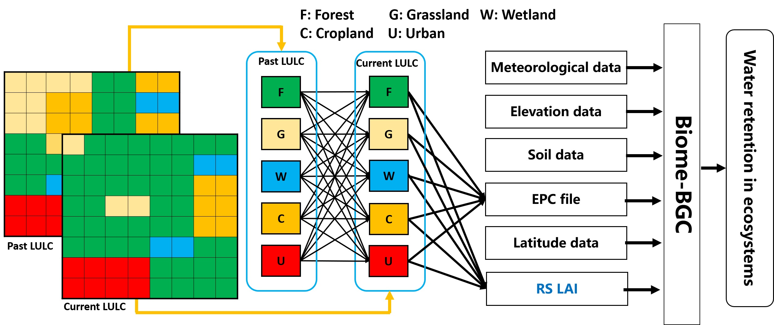
2.4. Framework of Integrating RS Time Series in Biome-BGC to Estimate WRE

In the original Biome-BGC model, the LAI was estimated from the model itself by multiplying leaf C (kg/m2 C) by specific leaf area (SLA) (m2/kg C) [76]. Leaf C is the total dry leaf mass C per unit area, while SLA is the leaf area per unit of dry leaf mass C [76,77]. However, the LAI estimated by Biome-BGC does not consider the vegetation structure of varied LULC change trajectories and disturbances (fire, pests and diseases) [55]. Thus, we used the remotely sensed LAI time series derived from MOD15A2H V6 as a surrogate. First, a modified temporal spatial filter was used to fill the gaps and replace lower-quality records with higher-quality records according to the quality control and filled value information [78]. Then, a Savitzky–Golay filter with a time window of 7 was used to smooth the LAI time series [79,80,81]. Finally, we interpolated the smoothed 8-day LAI time series into a daily LAI of one year (total 365 days) to meet the input needs of Biome-BGC.
Next, Equation (1) was used to calculate WRE based on water balance theory, and all required variables were the output variables from Biome-BGC (Figure 2):
W R E = k = 1 365 ( P R E k E T k S R k )
E T k = C E k + T k + L E k + S E k
S R k = { S W k S W s a t , | S W k > S W s a t 0.5 × ( S W k S W f c ) , | S W s a t S W k > S W f c 0 , | S W k S W f c
where P R E k is the precipitation on day k; E T k is the total evapotranspiration on day k; S R k is the stormwater runoff on day k; C E k is the canopy evaporation on day k; T k is the transpiration on day k; S E k is the soil evaporation on day k; L E k is the litter evaporation on day k; S W k is the soil water content on day k; S W s a t is the saturated soil water capacity; and S W f c is the field soil water capacity.
Multiple datasets were used as inputs to drive the Biome-BGC. Meanwhile, these datasets were varied in format, and spatial and temporal resolution. Thus, they were integrated to meet the needs of model input. First, all datasets were converted into raster grids via WGS84/Albers Equal Area Conic projection. Then, they were regrouped and resampled into a 1 km × 1 km grid for matching. Next, the spin-up run was used to produce the initial values of the water-state variables, which were saved in the restart files. Then, the normal run was used to model the hydrological process and export the hydrological variables. Finally, these output hydrological variables were used to calculate WRE based on Equations (1) and (2). In addition, we calibrated the eco-physiological parameters with local field data of prior studies in China, which would improve the performance of the Biome-BGC model in hydrological processes simulation. All eco-physiological parameters were obtained from the published literature and are given in Table S2.

2.5. Evaluating the Effect of Land Cover Changes on WRE

2.5.1. Model Performance Evaluation

To test the confidence of the simulated WRE, we compared our simulated ET with the ET results from the MOD16A2 product derived from Terra MODIS (https://earthexplorer.usgs.gov/ (accessed on 25 July 2021)) and the results from the CLSM (Catchment Land Surface Model) [82], VIC (Variable Infiltration Capacity Model) [83] and NOAH [84] derived from the Global Land Data Assimilation System (GLDAS) (https://ldas.gsfc.nasa.gov/gldas (accessed on 25 July 2021)) (Figure S2a). Meanwhile, we also compared the simulated SR we estimated and that estimated based on the methods of Gong et al. [1] and Hamel et al. [17]. The comparisons showed a good consistency among them (Figure S2b). In addition, we also compared the WRE capacity we estimated with other estimations that were conducted in the same climate region. All comparisons showed good consistency, indicating the feasibility of our results (Figure S2c).

2.5.2. Data Analysis

(1)
Quantifying LULC changes and their impact on WRE
Here, we created the LULC change map by overlaying the LULC map of 2015 onto the LULC map of 2000 for each pixel cell to track the LULC change trajectories (Figure 3). Meanwhile, we summarized LULC conversion categories, as shown in Table 2, for analysis of the results. To reveal the difference in vegetation structure across LULCs undergoing different LULC changes, we collect the annual maximum LAI of all pixels in each LULC. Then, we mapped the frequency distribution of annual maximum LAI in each LULC. Here, we used the maximum LAI rather than the mean or median LAI to highlight the size gap of LAI across LULCs with varied LULC change trajectories. In addition, we also added the median value line to better describe the difference in vegetation structure across different LULCs.
To quantify the impact of LULC change on WRE, we used the WRE map from 2015 minus the WRE map from 2000 to generate a map of WRE differences. Then, we used the LULC change map produced above to overlap the WRE difference map to compute the volume of WRE and WRE capacity across each LULC.
(2)
Determining factors that affect WRE based on random forest (RF) algorithm
The RF model is an ensemble learning method for regression based on constructing a multitude of decision trees to infer relationships between explanatory and response variables [85]. It has been widely used to address the influential predictors in large predictor sets in ecology-related studies [86,87,88]. Here, RF was used to identify the relative importance of different environmental factors in determining WRE. WRE obtained from each pixel was used as the target variable, while the maximum LAI, clay content (%), litter content (g/m2), annual total precipitation (mm) and slope calculated from DEM (°) were obtained from each pixel and were used as input variables. All these input variables were chosen by referring to prior studies that demonstrate which factors connect tightly with WRE [89,90]. Next, the ‘feature importance’ produced by RF was used to quantify the relative importance of different factors to WRE.
(3)
Using loess regression to fit a smooth curve between LAI and WRE/ET/SR
Loess regression is a regression method that creates a smooth line through a scatter plot, displaying the relationship between variables and helping readers to foresee trends [91]. Compared with other regression methods, loess regression does not require the specification of a function to fit a model to all data in the samples. Here, we used loess regression to fit a smooth curve between LAI and the WRE-related variables to better understand the dynamic response of LAI to WRE/ET/SR.

3. Results

3.1. LULC Change

Approximately 13.02% of LULC types changed between 2000 and 2015 (Figure 4b), and changed areas were evenly distributed across the entire area (Figure 4a). The forests and urban areas increased by approximately 4.15% (333.47 km2) and 53.17% (1170.26 km2) (Figure 4b), respectively, while wetlands and croplands declined by 34.19% (161.89 km2) and 27.02% (1301.66 km2), respectively (Figure 4b). Dramatic transfer in and transfer out occurred in different LULCs. Increased forests were mostly converted from cropland (364.76 km2), while forest loss was mostly owing to cropland expansion (52.83 km2) and urbanization (65.95 km2) (Figure 4b, Table S3). Likewise, increased urban areas were mostly converted from cropland (990.35 km2). Meanwhile, cropland expansion and urbanization were the main causes inducing the loss of wetlands (Figure 4b, Table S3).
Furthermore, the density distribution of the LAI was varied in LULCs with different LULC change trajectories. For forests, the LAI of unchanged forests was mainly distributed in the high-level range (4–6) (Figure 5). In contrast, the LAI of new forests converted from other LULCs mainly occurred in the low-level range (0–3) (Figure 5). Meanwhile, the LAI in grassland and cropland with different LULC change trajectories mainly occurred in the low-level range (0–3) (Figure 5).

3.2. The Impact of LULC Change on WRE

Compared with 2000, the volume of WRE in 2015 increased by approximately 8.58 million m3 (Figure 6b). Unchanged forests and new-planted forests contributed by approximately 14.46 million m3 and 12.28 million m3, respectively. Urbanization, cropland expansion and deforestation caused WRE to decline by 11.96 million m3, 5.86 million m3 and 3.20 million m3, respectively (Figure 6b). Areas that underwent dramatic WRE changes were mainly concentrated in western and northern Beijing (Figure 6a). Meanwhile, WRE capacity change varied in areas with different LULC change trajectories. WRE capacity per unit area improvement in new-planted forests (124.69 ± 14.30 m3/ha) was much greater than in unchanged forests (15.60 ± 7.85 m3/ha) (Figure 6c). Conversely, WRE capacity per unit area declined by approximately 143.92 ± 10.51 m3/ha and 131.31 ± 21.60 m3/ha in areas undergoing cropland expansion and urbanization, respectively (Figure 6c).

3.3. Effect of Varied LAI on WRE across Different LULCs

To understand the importance of different environmental factors in determining WRE, these factors were sorted based on RF. Under the condition of considering the remotely sensed LAI in Biome-BGC, Table 3 shows that the LAI was the most important factor (RF score was 2.12). Clay content (%) (RF score was 0.97) and litter ranked as the second (RF score was 0.65) and third most important factors, respectively.
In addition, we compared the response of ET, SR and WRE with LAI dynamics in different LULCs. CE increased with increasing LAI but with varied slopes in all LULCs (Figure 7). Transpiration also increased with the rising LAI except in forests, in which transpiration gradually became saturated when the LAI was over 4 (Figure 7). Conversely, SE decreased with increasing LAI with varied slopes. LE decreased with increasing LAI but gradually became saturated (Figure 7). SR also decreased with increasing LAI with varied slopes in different LULCs. Specifically, SR decreased with an LAI of less than 4 but was depleted after that in forests. The response of WRE to the LAI varied across different LULCs. In forests, the WRE increased with increasing LAI until 4 but decreased after the LAI exceeded 4. However, WRE increased slowly with increasing LAI at various rates in other LULCs (Figure 7).

4. Discussion

4.1. Contribution of Forests to WRE

The results show that forests are important in guaranteeing regional water resource security; they use less than 30% of the total area but contribute over half of the total WRE (Table S3, Figure S5). This was mostly related to a higher WRE capacity in forests than other LULCs. Compared with forests, the simpler species structure and composition in grassland and cropland caused a lower LAI (Figure 5). The varied LAI among different LULCs is probably the main cause explaining the divergence of WRE capacity (Table 3, Figure 5). Meanwhile, the increased volume of WRE contributed by unchanged forests (14.46 million m3) was much greater than that of new-planted forests (12.28 million m3), but the increase in WRE capacity per unit area in new-planted forests (124.69 ± 14.30 m3/ha) was much greater than that of unchanged forests (15.60 ± 7.85 m3/ha). Unchanged forests hold higher LAI and grow faster to cause more ET, which was probably the main factor to explain the lesser WRE capacity improvement compared with new-planted forests (Figure 7, Figure S4 and Figure S8). Thus, afforestation would probably quickly increase the volume of WRE in an area.
Although the WRE capacity in most new-planted forests was lower than that of unchanged forests (Figure 7), WRE capacity continued to improve with vegetation growth. New-planted trees occur mostly due to restoration efforts, which are usually of a single species. These artificially planted trees are dominated by poplar and pine and are far from mature [92,93,94]. Young stand age, homogenized species and sparse understory vegetation commonly result in a low LAI [88]. New-planted forests will continue to grow with time, probably for decades. The continued growth of forests inducing increased LAI leads to increased WRE. Nonetheless, the inverted U-shape relationship between LAI and WRE in forests implies that growth did not always promote the increase in WRE (Figure 7 and Figure S8). Although complex canopy structure is more efficient to intercept rainwater to reduce SR, it becomes saturated after forest growth enters a certain stage (Figure 7). ET continues to increase with rising LAI, which in turn causes a decrease in WRE (Figure 7). Prior studies have already demonstrated that the increase in LAI causes more ET after restoration, which leads to a decline in soil water [95,96,97]. Furthermore, the soil water consumption was gradually aggravated along with the increasing forest age, in particular, after 30–35 years of plantation [98,99,100]. Excessive consumption of soil water was the most important reason for the wilt or mortality of forests [101].
Debate exists as to whether forests increase or reduce water resources over a long period [102]. Although previous studies have consistently concluded that increasing forest coverage would decrease SR to reduce total runoff [103,104,105], contradictions have mainly focused on the relationship between forests and baseflow. Some studies proposed that forest decreases WRE, which in turn reduces baseflow [106], while others concluded that forest would increase WRE to promote baseflow [107,108,109]. Indeed, the relationship between forests and WRE is the result of the composite effect of climate, terrain, vegetation and soil [110,111,112]. The relationship between forests and WRE will change as the forest age increases [2,113]. Moreover, the impact of forest age on WRE will be aggravated in rainwater-limited areas such as Beijing [13,114]. Thus, to reduce the possible risk of declining WRE, slow-growth tree species with higher water use efficiency should be given priority over exotic species during restoration [115,116].

4.2. Remotely Sensed LAI Role in Biome-BGC

Integrating remotely sensed LAI into Biome-BGC is an efficient way to describe the impact of LULC change with varied vegetation structures on WRE. LAI estimated from Biome-BGC was controlled by climate, terrain, soil and vegetation types but did not consider the impact of LULC change trajectories [55,117]. Thus, it was difficult to describe the spatial information of the vegetation structure owing to varied LULC change trajectories, causing LAI estimated from Biome-BGC to be distant from reality (Figures S6 and S7). In contrast, the remotely sensed LAI can capture the long-term dynamics in vegetation structure, and especially in capturing the difference in vegetation structure of unchanged old forests and increased forests (Figure S6). The fact that the importance score of remotely sensed LAI was higher than modelled LAI in determining WRE implied that integrating remotely sensed LAI into Biome-BGC is helpful to describe the constraint of vegetation on hydrological processes (Table 3, Figures S6 and S7). Prior studies also demonstrated that remotely sensed LAI was efficient to describe canopy structure information, which has been used in hydrological variable inversion [48,118,119]. Remotely sensed LAI provides long-time-series, multi-temporal, high-resolution and stable images. Although field surveys and experiments probably obtain more direct and confident LAI, shortages of time and funding restrict the application of field surveys to large areas. Conversely, indirectly measured remotely sensed LAI offers a comprehensive understanding of the landscape at a regional scale. Additionally, the addition of a litter water module could help perfect the water cycle process. Litter increases water interception and infiltration [71,120], and it also reduces surface runoff and soil erosion, especially in old-growth forests [71].
However, the limitation of remotely sensed LAI is that it is difficult to capture accurate information on understory vegetation [121,122]. The understory vegetation would induce higher ET and intercept more precipitation to reduce the SR. Thus, our results probably underestimate the ET and overestimate the SR. It is still unclear whether these opposite effects on WRE would be counteracted totally. In most cases, the size and biomass of understory vegetation are much lower than those of canopy vegetation [123,124,125]. The effect of understory vegetation on WRE might be limited [126,127,128]. Some studies have implied that Lidar has a stronger canopy penetration ability and the potential to detect information on understory vegetation [129]. However, high acquisition costs and low availability restrict its application, especially in developing countries [130]. In future, we will attempt to build the relationship between canopy structure and understory vegetation [131] based on measured data. Meanwhile, we will modify EPM to include processes that consider the understory vegetation structure and its impact on hydrological processes.

5. Conclusions

Previous studies that focused on the impact of LULC change on WRE neglected the effect of varied vegetation structures. This neglect has hampered a more comprehensive acknowledgment of the impact of LULC changes on WRE. In this study, we integrated remotely sensed LAI into the ecosystem process-based Biome-BGC to analyse the impact of LULC changes on WRE in Beijing between 2000 and 2015, including consideration of the varied vegetation structures. We found that the volume of WRE in 2015 increased by approximately 8.58 million m3 compared with 2000. Unchanged forests and new-planted forests contributed approximately 14.46 million m3 and 12.28 million m3, respectively. In contrast, urbanization, cropland expansion and deforestation caused WRE to decline by 11.96 million m3, 5.86 million m3 and 3.20 million m3, respectively. Although the increased WRE contributed by unchanged forests (14.46 million m3) was much more than that of new-planted forests (12.28 million m3), the increase in WRE capacity per unit area in new-planted forests (124.69 ± 14.30 m3/ha) was much greater than that of unchanged forests (15.60 ± 7.85 m3/ha). Higher LAI in unchanged forests induced more ET, which was the main cause leading to the lower WRE capacity per unit area. Our results suggest that the effect of vegetation structure on WRE cannot be ignored. Integrating the remotely sensed LAI with Biome-BGC was efficient in analysing the effect of varied vegetation structures when quantifying the impact of LULC change on WRE. Furthermore, our approach can be used to better understand the comprehensive results of the impact of LULC change on WRE and guide land use policies to maintain or increase regionally available water resources.

Supplementary Materials

The following supporting information can be downloaded at: https://www.mdpi.com/article/10.3390/rs14030743/s1, Figure S1: (a) Correlation between LAI and litter mass; (b) correlation between litter mass and maximum litter water content; Figure S2: (a) Comparison of Biome-BGC ET vs CLSM, VIC, NOAH2 and MODIS ET; (b) Comparison of simulated SR from this study and that estimated based on the mothed of Gong et al. (2017) and Hamel et al. (2020); (c) Comparison of simulated WRE from this study and that from Pan et al. (2021) and Li et al. (2000); Figure S3: (a) Spatial distribution of meteorological stations; (b) Comparison of gridded precipitation vs. station observed precipitation (mm/day); Figure S4: Spatial distribution of WRE capacity (m3/ha) in (a) 2000 and (b) 2015; Figure S5: The volume of WRE (×106 m3) in 2015 contributed by different LULCs; Figure S6: The comparisons of three LAIs among (a) unchanged forests and (b) increased forests; Figure S7: The comparisons of yearly mean smoothed satellite LAI VS simulated LAI in 2015; Figure S8: LAI and WRE change across unchanged and increased forests between 2000 and 2015; Table S1: LULC categories; Table S2: Eco-physiological parameters of the Biome-BGC model; Table S3: LULC conversion in Beijing between 2000 and 2015 (km2).

Author Contributions

Conceptualization, B.H. and X.W. (Xiaoke Wang); methodology, B.H.; validation, B.H., Y.Y. and H.Z.; writing—original draft preparation, B.H. and X.W. (Xiaoke Wang); writing—review and editing, Y.Y., R.L., H.Z., X.W. (Xuming Wang), X.W. (Xiaoke Wang) and Y.Z.; project administration, X.W. (Xiaoke Wang); funding acquisition, X.W. (Xiaoke Wang). All authors have read and agreed to the published version of the manuscript.

Funding

This research is supported by National Key Research and Development Program of China (No. 2018YFC0507303).

Institutional Review Board Statement

Not applicable.

Informed Consent Statement

Not applicable.

Data Availability Statement

The data presented in this study are available on request from the corresponding author.

Conflicts of Interest

The authors declare no conflict of interest.

References

  1. Gong, S.H.; Xiao, Y.; Xiao, Y.; Zhang, L.; Ouyang, Z.Y. Driving forces and their effects on water conservation services in forest ecosystems in China. Chin. Geogr. Sci. 2017, 27, 216–228. [Google Scholar] [CrossRef] [Green Version]
  2. Teixeira, G.M.; Figueiredo, P.H.A.; Salemi, L.F.; Ferraz, S.F.B.; Ranzini, M.; Arcova, F.C.S.; de Cicco, V.; Rizzi, N.E. Regeneration of tropical montane cloud forests increases water yield in the Brazilian Atlantic Forest. Ecohydrology 2021, 14, e2298. [Google Scholar] [CrossRef]
  3. Wang, X.; Shen, H.; Li, X.; Jing, F. Concepts, processes and quantification methods of the forest water conservation at the multiple scales. Shengtai Xuebao Acta Ecol. Sin. 2013, 33, 1019–1030. [Google Scholar] [CrossRef]
  4. Ouyang, Z.; Zheng, H.; Xiao, Y.; Polasky, S.; Liu, J.; Xu, W.; Wang, Q.; Zhang, L.; Xiao, Y.; Rao, E.; et al. Improvements in ecosystem services from investments in natural capital. Science 2016, 352, 1455–1459. [Google Scholar] [CrossRef] [PubMed]
  5. Dong, T.; Xu, W.; Zheng, H.; Xiao, Y.; Kong, L.; Ouyang, Z. A Framework for Regional Ecological Risk Warning Based on Ecosystem Service Approach: A Case Study in Ganzi, China. Sustainability 2018, 10, 2699. [Google Scholar] [CrossRef] [Green Version]
  6. Kong, L.; Zheng, H.; Xiao, Y.; Ouyang, Z.; Li, C.; Zhang, J.; Huang, B. Mapping Ecosystem Service Bundles to Detect Distinct Types of Multifunctionality within the Diverse Landscape of the Yangtze River Basin, China. Sustainability 2018, 10, 857. [Google Scholar] [CrossRef] [Green Version]
  7. Hou, G.; Delang, C.O.; Lu, X. Afforestation changes soil organic carbon stocks on sloping land: The role of previous land cover and tree type. Ecol. Eng. 2020, 152, 105860. [Google Scholar] [CrossRef]
  8. Gage, E.A.; Cooper, D.J. Urban forest structure and land cover composition effects on land surface temperature in a semi-arid suburban area. Urban For. Urban Green. 2017, 28, 28–35. [Google Scholar] [CrossRef]
  9. Fortuny, X.; Chauchard, S.; Carcaillet, C. Confounding legacies of land uses and land-form pattern on the regional vegetation structure and diversity of Mediterranean montane forests. For. Ecol. Manag. 2017, 384, 268–278. [Google Scholar] [CrossRef]
  10. Requena-Mullor, J.M.; Quintas-Soriano, C.; Brandt, J.; Cabello, J.; Castro, A.J. Modeling how land use legacy affects the provision of ecosystem services in Mediterranean southern Spain. Environ. Res. Lett. 2018, 13, 114008. [Google Scholar] [CrossRef] [Green Version]
  11. Dennedy-Frank, P.J.; Gorelick, S.M. Insights from watershed simulations around the world: Watershed service-based restoration does not significantly enhance streamflow. Glob. Environ. Chang. 2019, 58, 101938. [Google Scholar] [CrossRef]
  12. Zhao, M.; Zhang, J.; Velicogna, I.; Liang, C.; Li, Z. Ecological restoration impact on total terrestrial water storage. Nat. Sustain. 2021, 4, 56–62. [Google Scholar] [CrossRef]
  13. Tian, A.; Wang, Y.; Webb, A.A.; Liu, Z.; Ma, J.; Yu, P.; Wang, X. Water yield variation with elevation, tree age and density of larch plantation in the Liupan Mountains of the Loess Plateau and its forest management implications. Sci. Total Environ. 2021, 752, 141752. [Google Scholar] [CrossRef] [PubMed]
  14. Winkler, K.; Fuchs, R.; Rounsevell, M.; Herold, M. Global land use changes are four times greater than previously estimated. Nat. Commun. 2021, 12, 2501. [Google Scholar] [CrossRef] [PubMed]
  15. Potapov, P.; Hansen, M.C.; Laestadius, L.; Turubanova, S.; Yaroshenko, A.; Thies, C.; Smith, W.; Zhuravleva, I.; Komarova, A.; Minnemeyer, S.; et al. The last frontiers of wilderness: Tracking loss of intact forest landscapes from 2000 to 2013. Sci. Adv. 2017, 3, e1600821. [Google Scholar] [CrossRef] [Green Version]
  16. Wang, X.; Zou, Z.; Zou, H. Water quality evaluation of Haihe River with fuzzy similarity measure methods. J. Environ. Sci. 2013, 25, 2041–2046. [Google Scholar] [CrossRef]
  17. Hamel, P.; Valencia, J.; Schmitt, R.; Shrestha, M.; Piman, T.; Sharp, R.P.; Francesconi, W.; Guswa, A.J. Modeling seasonal water yield for landscape management: Applications in Peru and Myanmar. J. Environ. Manag. 2020, 270, 110792. [Google Scholar] [CrossRef]
  18. Ouyang, Z.; Song, C.; Zheng, H.; Polasky, S.; Xiao, Y.; Bateman, I.J.; Liu, J.; Ruckelshaus, M.; Shi, F.; Xiao, Y.; et al. Using gross ecosystem product (GEP) to value nature in decision making. Proc. Natl. Acad. Sci. USA 2020, 117, 14593. [Google Scholar] [CrossRef]
  19. Kimball, J.S.; White, M.A.; Running, S.W. BIOME-BGC simulations of stand hydrologic processes for BOREAS. J. Geophys. Res. Atmos. 1997, 102, 29043–29051. [Google Scholar] [CrossRef]
  20. Abbaspour, K.C.; Rouholahnejad, E.; Vaghefi, S.; Srinivasan, R.; Yang, H.; Kløve, B. A continental-scale hydrology and water quality model for Europe: Calibration and uncertainty of a high-resolution large-scale SWAT model. J. Hydrol. 2015, 524, 733–752. [Google Scholar] [CrossRef] [Green Version]
  21. Lombardozzi, D.L.; Zeppel, M.J.B.; Fisher, R.A.; Tawfik, A. Representing nighttime and minimum conductance in CLM4.5: Global hydrology and carbon sensitivity analysis using observational constraints. Geosci. Model Dev. 2017, 10, 321–331. [Google Scholar] [CrossRef] [Green Version]
  22. VanShaar, J.R.; Haddeland, I.; Lettenmaier, D.P. Effects of land-cover changes on the hydrological response of interior Columbia River basin forested catchments. Hydrol. Processes 2002, 16, 2499–2520. [Google Scholar] [CrossRef]
  23. Tang, J.; Miller, P.A.; Crill, P.M.; Olin, S.; Pilesjö, P. Investigating the influence of two different flow routing algorithms on soil–water–vegetation interactions using the dynamic ecosystem model LPJ-GUESS. Ecohydrology 2015, 8, 570–583. [Google Scholar] [CrossRef]
  24. Zhang, Z.; Huang, M.; Yang, Y.; Zhao, X. Evaluating drought-induced mortality risk for Robinia pseudoacacia plantations along the precipitation gradient on the Chinese Loess Plateau. Agric. For. Meteorol. 2020, 284, 107897. [Google Scholar] [CrossRef]
  25. Zhang, H.; Wang, B.; Liu, D.L.; Zhang, M.; Leslie, L.M.; Yu, Q. Using an improved SWAT model to simulate hydrological responses to land use change: A case study of a catchment in tropical Australia. J. Hydrol. 2020, 585, 124822. [Google Scholar] [CrossRef]
  26. Hazarika, M.K.; Yasuoka, Y.; Ito, A.; Dye, D. Estimation of net primary productivity by integrating remote sensing data with an ecosystem model. Remote Sens. Environ. 2005, 94, 298–310. [Google Scholar] [CrossRef]
  27. Ma, R.; Zhang, L.; Tian, X.; Zhang, J.; Yuan, W.; Zheng, Y.; Zhao, X.; Kato, T. Assimilation of Remotely-Sensed Leaf Area Index into a Dynamic Vegetation Model for Gross Primary Productivity Estimation. Remote Sens. 2017, 9, 188. [Google Scholar] [CrossRef] [Green Version]
  28. Seo, H.; Kim, Y. Role of remotely sensed leaf area index assimilation in eco-hydrologic processes in different ecosystems over East Asia with Community Land Model version 4.5–Biogeochemistry. J. Hydrol. 2021, 594, 125957. [Google Scholar] [CrossRef]
  29. Cortés, J.; Mahecha, M.D.; Reichstein, M.; Myneni, R.B.; Chen, C.; Brenning, A. Where Are Global Vegetation Greening and Browning Trends Significant? Geophys. Res. Lett. 2021, 48, e2020GL091496. [Google Scholar] [CrossRef]
  30. Chen, Y.; Guerschman, J.P.; Cheng, Z.; Guo, L. Remote sensing for vegetation monitoring in carbon capture storage regions: A review. Appl. Energy 2019, 240, 312–326. [Google Scholar] [CrossRef]
  31. Wang, Y.; Li, G.; Ding, J.; Guo, Z.; Tang, S.; Wang, C.; Huang, Q.; Liu, R.; Chen, J.M. A combined GLAS and MODIS estimation of the global distribution of mean forest canopy height. Remote Sens. Environ. 2016, 174, 24–43. [Google Scholar] [CrossRef]
  32. Cui, L.; Jiao, Z.; Dong, Y.; Sun, M.; Zhang, X.; Yin, S.; Ding, A.; Chang, Y.; Guo, J.; Xie, R. Estimating Forest Canopy Height Using MODIS BRDF Data Emphasizing Typical-Angle Reflectances. Remote Sens. 2019, 11, 2239. [Google Scholar] [CrossRef] [Green Version]
  33. Yu, Z.; Zhao, H.; Liu, S.; Zhou, G.; Fang, J.; Yu, G.; Tang, X.; Wang, W.; Yan, J.; Wang, G.; et al. Mapping forest type and age in China’s plantations. Sci. Total Environ. 2020, 744, 140790. [Google Scholar] [CrossRef] [PubMed]
  34. Spracklen, B.; Spracklen, D.V. Synergistic Use of Sentinel-1 and Sentinel-2 to Map Natural Forest and Acacia Plantation and Stand Ages in North-Central Vietnam. Remote Sens. 2021, 13, 185. [Google Scholar] [CrossRef]
  35. Yang, H.; Ciais, P.; Santoro, M.; Huang, Y.; Li, W.; Wang, Y.; Bastos, A.; Goll, D.; Arneth, A.; Anthoni, P.; et al. Comparison of forest above-ground biomass from dynamic global vegetation models with spatially explicit remotely sensed observation-based estimates. Glob. Chang. Biol. 2020, 26, 3997–4012. [Google Scholar] [CrossRef]
  36. Ding, L.; Li, Z.; Shen, B.; Wang, X.; Xu, D.; Yan, R.; Yan, Y.; Xin, X.; Xiao, J.; Li, M.; et al. Spatial patterns and driving factors of aboveground and belowground biomass over the eastern Eurasian steppe. Sci. Total Environ. 2022, 803, 149700. [Google Scholar] [CrossRef]
  37. Konings, A.G.; Saatchi, S.S.; Frankenberg, C.; Keller, M.; Leshyk, V.; Anderegg, W.R.L.; Humphrey, V.; Matheny, A.M.; Trugman, A.; Sack, L.; et al. Detecting forest response to droughts with global observations of vegetation water content. Glob. Chang. Biol. 2021, 27, 6005–6024. [Google Scholar] [CrossRef] [PubMed]
  38. Miller, D.L.; Alonzo, M.; Meerdink, S.K.; Allen, M.A.; Tague, C.L.; Roberts, D.A.; McFadden, J.P. Seasonal and interannual drought responses of vegetation in a California urbanized area measured using complementary remote sensing indices. ISPRS J. Photogramm. Remote Sens. 2022, 183, 178–195. [Google Scholar] [CrossRef]
  39. Zhang, Y.; Song, C.; Zhang, K.; Cheng, X.; Band, L.E.; Zhang, Q. Effects of land use/land cover and climate changes on terrestrial net primary productivity in the Yangtze River Basin, China, from 2001 to 2010. J. Geophys. Res. Biogeosci. 2014, 119, 1092–1109. [Google Scholar] [CrossRef]
  40. Shen, W.; Li, M.; Huang, C.; Tao, X.; Li, S.; Wei, A. Mapping Annual Forest Change Due to Afforestation in Guangdong Province of China Using Active and Passive Remote Sensing Data. Remote Sens. 2019, 11, 490. [Google Scholar] [CrossRef] [Green Version]
  41. Valtonen, A.; Korkiatupa, E.; Holm, S.; Malinga, G.M.; Nakadai, R. Remotely sensed vegetation greening along a restoration gradient of a tropical forest, Kibale National Park, Uganda. Land Degrad. Dev. 2021, 11, 4096. [Google Scholar] [CrossRef]
  42. Wu, C.; Peng, D.; Soudani, K.; Siebicke, L.; Gough, C.M.; Arain, M.A.; Bohrer, G.; Lafleur, P.M.; Peichl, M.; Gonsamo, A.; et al. Land surface phenology derived from normalized difference vegetation index (NDVI) at global FLUXNET sites. Agric. For. Meteorol. 2017, 233, 171–182. [Google Scholar] [CrossRef]
  43. Tian, J.; Zhu, X.; Chen, J.; Wang, C.; Shen, M.; Yang, W.; Tan, X.; Xu, S.; Li, Z. Improving the accuracy of spring phenology detection by optimally smoothing satellite vegetation index time series based on local cloud frequency. ISPRS J. Photogramm. Remote Sens. 2021, 180, 29–44. [Google Scholar] [CrossRef]
  44. Deng, Y.; Li, X.; Shi, F.; Hu, X. Woody plant encroachment enhanced global vegetation greening and ecosystem water-use efficiency. Glob. Ecol. Biogeogr. 2021, 30, 2337–2353. [Google Scholar] [CrossRef]
  45. Ju, W.; Gao, P.; Zhou, Y.; Chen, J.M.; Chen, S.; Li, X. Prediction of summer grain crop yield with a process-based ecosystem model and remote sensing data for the northern area of the Jiangsu Province, China. Int. J. Remote Sens. 2010, 31, 1573–1587. [Google Scholar] [CrossRef]
  46. Viskari, T.; Hardiman, B.; Desai, A.R.; Dietze, M.C. Model-data assimilation of multiple phenological observations to constrain and predict leaf area index. Ecol. Appl. 2015, 25, 546–558. [Google Scholar] [CrossRef]
  47. Wang, Q.; Watanabe, M.; Ouyang, Z. Simulation of water and carbon fluxes using BIOME-BGC model over crops in China. Agric. For. Meteorol. 2005, 131, 209–224. [Google Scholar] [CrossRef]
  48. Yan, H.; Wang, S.Q.; Billesbach, D.; Oechel, W.; Zhang, J.H.; Meyers, T.; Martin, T.A.; Matamala, R.; Baldocchi, D.; Bohrer, G.; et al. Global estimation of evapotranspiration using a leaf area index-based surface energy and water balance model. Remote Sens. Environ. 2012, 124, 581–595. [Google Scholar] [CrossRef] [Green Version]
  49. Zhang, Y.; Huang, M.; Lian, J. Spatial distributions of optimal plant coverage for the dominant tree and shrub species along a precipitation gradient on the central Loess Plateau. Agric. For. Meteorol. 2015, 206, 69–84. [Google Scholar] [CrossRef]
  50. Wu, Y.; Wang, X.; Ouyang, S.; Xu, K.; Hawkins, B.A.; Sun, O.J. A test of BIOME-BGC with dendrochronology for forests along the altitudinal gradient of Mt. Changbai in northeast China. J. Plant Ecol. 2017, 10, 415–425. [Google Scholar] [CrossRef] [Green Version]
  51. Zhou, C.; Fu, B.; Wang, X.; Yin, L.; Feng, X. The Regional Impact of Ecological Restoration in the Arid Steppe on Dust Reduction over the Metropolitan Area in Northeastern China. Environ. Sci. Technol. 2020, 54, 7775–7786. [Google Scholar] [CrossRef]
  52. Liu, B.J.; Zhang, L.; Lu, F.; Deng, L.; Zhao, H.; Luo, Y.J.; Liu, X.P.; Zhang, K.R.; Wang, X.K.; Liu, W.W.; et al. Greenhouse gas emissions and net carbon sequestration of the Beijing-Tianjin Sand Source Control Project in China. J. Clean. Prod. 2019, 225, 163–172. [Google Scholar] [CrossRef]
  53. Yu, Z.; Liu, X.; Zhang, J.; Xu, D.; Cao, S. Evaluating the net value of ecosystem services to support ecological engineering: Framework and a case study of the Beijing Plains afforestation project. Ecol. Eng. 2018, 112, 148–152. [Google Scholar] [CrossRef]
  54. Yao, N.; Konijnendijk van den Bosch, C.C.; Yang, J.; Devisscher, T.; Wirtz, Z.; Jia, L.; Duan, J.; Ma, L. Beijing’s 50 million new urban trees: Strategic governance for large-scale urban afforestation. Urban For. Urban Green. 2019, 44, 126392. [Google Scholar] [CrossRef]
  55. Thornton, P.E.; Rosenbloom, N.A. Ecosystem model spin-up: Estimating steady state conditions in a coupled terrestrial carbon and nitrogen cycle model. Ecol. Model. 2005, 189, 25–48. [Google Scholar] [CrossRef]
  56. Pietsch, S.A.; Hasenauer, H.; Kučera, J.; Čermák, J. Modeling effects of hydrological changes on the carbon and nitrogen balance of oak in floodplains. Tree Physiol. 2003, 23, 735–746. [Google Scholar] [CrossRef] [Green Version]
  57. Eastaugh, C.S.; Pötzelsberger, E.; Hasenauer, H. Assessing the impacts of climate change and nitrogen deposition on Norway spruce (Picea abies L. Karst) growth in Austria with BIOME-BGC. Tree Physiol. 2011, 31, 262–274. [Google Scholar] [CrossRef] [Green Version]
  58. Du, L.; Zeng, Y.; Ma, L.; Qiao, C.; Wu, H.; Su, Z.; Bao, G. Effects of anthropogenic revegetation on the water and carbon cycles of a desert steppe ecosystem. Agric. For. Meteorol. 2021, 300, 108339. [Google Scholar] [CrossRef]
  59. Zhou, X.; Xin, Q.; Dai, Y.; Li, W. A deep-learning-based experiment for benchmarking the performance of global terrestrial vegetation phenology models. Glob. Ecol. Biogeogr. 2021, 30, 2178–2199. [Google Scholar] [CrossRef]
  60. You, Y.; Wang, S.; Ma, Y.; Wang, X.; Liu, W. Improved Modeling of Gross Primary Productivity of Alpine Grasslands on the Tibetan Plateau Using the Biome-BGC Model. Remote Sens. 2019, 11, 1287. [Google Scholar] [CrossRef] [Green Version]
  61. Yan, M.; Li, Z.; Tian, X.; Zhang, L.; Zhou, Y. Improved simulation of carbon and water fluxes by assimilating multi-layer soil temperature and moisture into process-based biogeochemical model. For. Ecosyst. 2019, 6, 12. [Google Scholar] [CrossRef] [Green Version]
  62. Smeglin, Y.H.; Davis, K.J.; Shi, Y.; Eissenstat, D.M.; Kaye, J.P.; Kaye, M.W. Observing and Simulating Spatial Variations of Forest Carbon Stocks in Complex Terrain. J. Geophys. Res. Biogeosci. 2020, 125, e2019JG005160. [Google Scholar] [CrossRef]
  63. Ichii, K.; Hashimoto, H.; White, M.A.; Potter, C.; Hutyra, L.R.; Huete, A.R.; Myneni, R.B.; Nemani, R.R. Constraining rooting depths in tropical rainforests using satellite data and ecosystem modeling for accurate simulation of gross primary production seasonality. Glob. Change Biol. 2007, 13, 67–77. [Google Scholar] [CrossRef]
  64. Sanchez-Ruiz, S.; Chiesi, M.; Fibbi, L.; Carrara, A.; Maselli, F.; Gilabert, M.A. Optimized Application of Biome-BGC for Modeling the Daily GPP of Natural Vegetation Over Peninsular Spain. J. Geophys. Res. Biogeosci. 2018, 123, 531–546. [Google Scholar] [CrossRef]
  65. Yan, M.; Tian, X.; Li, Z.; Chen, E.; Wang, X.; Han, Z.; Sun, H. Simulation of Forest Carbon Fluxes Using Model Incorporation and Data Assimilation. Remote Sens. 2016, 8, 567. [Google Scholar] [CrossRef] [Green Version]
  66. Tian, X.; Yan, M.; van der Tol, C.; Li, Z.; Su, Z.; Chen, E.; Li, X.; Li, L.; Wang, X.; Pan, X.; et al. Modeling forest above-ground biomass dynamics using multi-source data and incorporated models: A case study over the qilian mountains. Agric. For. Meteorol. 2017, 246, 1–14. [Google Scholar] [CrossRef]
  67. Running, S.W.; Coughlan, J.C. A general model of forest ecosystem processes for regional applications I. Hydrologic balance, canopy gas exchange and primary production processes. Ecol. Model. 1988, 42, 125–154. [Google Scholar] [CrossRef]
  68. Jarvis, P.G.; Monteith, J.L.; Weatherley, P.E. The interpretation of the variations in leaf water potential and stomatal conductance found in canopies in the field. Philos. Trans. R. Soc. London. B Biol. Sci. 1976, 273, 593–610. [Google Scholar] [CrossRef]
  69. Ueyama, M.; Ichii, K.; Hirata, R.; Takagi, K.; Asanuma, J.; Machimura, T.; Nakai, Y.; Ohta, T.; Saigusa, N.; Takahashi, Y.; et al. Simulating carbon and water cycles of larch forests in East Asia by the BIOME-BGC model with AsiaFlux data. Biogeosciences 2010, 7, 959–977. [Google Scholar] [CrossRef] [Green Version]
  70. Zhang, Y.-W.; Wang, K.-B.; Wang, J.; Liu, C.; Shangguan, Z.-P. Changes in soil water holding capacity and water availability following vegetation restoration on the Chinese Loess Plateau. Sci. Rep. 2021, 11, 9692. [Google Scholar] [CrossRef]
  71. Xia, L.; Song, X.; Fu, N.; Cui, S.; Li, L.; Li, H.; Li, Y. Effects of forest litter cover on hydrological response of hillslopes in the Loess Plateau of China. CATENA 2019, 181, 104076. [Google Scholar] [CrossRef]
  72. Wang, L.; Zhang, G.; Zhu, P.; Wang, X. Comparison of the effects of litter covering and incorporation on infiltration and soil erosion under simulated rainfall. Hydrol. Processes 2020, 34, 2911–2922. [Google Scholar] [CrossRef]
  73. Zhang, Q.; Sun, R.; Jiang, G.; Xu, Z.; Liu, S. Carbon and energy flux from a Phragmites australis wetland in Zhangye oasis-desert area, China. Agric. For. Meteorol. 2016, 230–231, 45–57. [Google Scholar] [CrossRef]
  74. Glassy, J.M.; Running, S.W. Validating Diurnal Climatology Logic of the MT-CLIM Model Across a Climatic Gradient in Oregon. Ecol Appl 1994, 4, 248–257. [Google Scholar] [CrossRef] [Green Version]
  75. Zhang, L.; Li, X.; Yuan, Q.; Liu, Y. Object-based approach to national land cover mapping using HJ satellite imagery. J. Appl. Remote Sens. 2014, 8, 083686. [Google Scholar] [CrossRef]
  76. Thornton, P.E. Theoretical Framework of Biome-BGC Version 4.2. 2020. Available online: https://www.ntsg.umt.edu/files/biome-bgc/Golinkoff_BiomeBGCv4.2_TheoreticalBasis_1_18_10.pdf (accessed on 12 June 2021).
  77. Fang, H.; Baret, F.; Plummer, S.; Schaepman-Strub, G. An Overview of Global Leaf Area Index (LAI): Methods, Products, Validation, and Applications. Rev. Geophys. 2019, 57, 739–799. [Google Scholar] [CrossRef]
  78. Fang, H.; Liang, S.; Townshend, J.R.; Dickinson, R.E. Spatially and temporally continuous LAI data sets based on an integrated filtering method: Examples from North America. Remote Sens. Environ. 2008, 112, 75–93. [Google Scholar] [CrossRef]
  79. Jönsson, P.; Eklundh, L. TIMESAT—a program for analyzing time-series of satellite sensor data. Comput. Geosci. 2004, 30, 833–845. [Google Scholar] [CrossRef] [Green Version]
  80. Yuan, H.; Dai, Y.; Xiao, Z.; Ji, D.; Shangguan, W. Reprocessing the MODIS Leaf Area Index products for land surface and climate modelling. Remote Sens. Environ. 2011, 115, 1171–1187. [Google Scholar] [CrossRef]
  81. Xiao, Z.; Liang, S.; Wang, J.; Jiang, B.; Li, X. Real-time retrieval of Leaf Area Index from MODIS time series data. Remote Sens. Environ. 2011, 115, 97–106. [Google Scholar] [CrossRef]
  82. Reichle, R.H.; Koster, R.D. Global assimilation of satellite surface soil moisture retrievals into the NASA Catchment land surface model. Geophys. Res. Lett. 2005, 32, 700. [Google Scholar] [CrossRef]
  83. Cherkauer, K.A.; Bowling, L.C.; Lettenmaier, D.P. Variable infiltration capacity cold land process model updates. Glob. Planet. Chang. 2003, 38, 151–159. [Google Scholar] [CrossRef]
  84. Niu, G.-Y.; Yang, Z.-L.; Mitchell, K.E.; Chen, F.; Ek, M.B.; Barlage, M.; Kumar, A.; Manning, K.; Niyogi, D.; Rosero, E.; et al. The community Noah land surface model with multiparameterization options (Noah-MP): 1. Model description and evaluation with local-scale measurements. J. Geophys. Res. Atmos. 2011, 116, D12109. [Google Scholar] [CrossRef] [Green Version]
  85. Breiman, L. Random Forests. Mach. Learn. 2001, 45, 5–32. [Google Scholar] [CrossRef] [Green Version]
  86. Chen, S.; Richer-de-Forges, A.C.; Leatitia Mulder, V.; Martelet, G.; Loiseau, T.; Lehmann, S.; Arrouays, D. Digital mapping of the soil thickness of loess deposits over a calcareous bedrock in central France. Catena 2021, 198, 105062. [Google Scholar] [CrossRef]
  87. Li, H.; Liu, L.; Koppa, A.; Shan, B.; Liu, X.; Li, X.; Niu, Q.; Cheng, L.; Miralles, D. Vegetation greening concurs with increases in dry season water yield over the Upper Brahmaputra River basin. J. Hydrol. 2021, 603, 126981. [Google Scholar] [CrossRef]
  88. Wang, M.; Liu, Q.; Pang, X. Evaluating ecological effects of roadside slope restoration techniques: A global meta-analysis. J. Environ. Manag. 2021, 281, 111867. [Google Scholar] [CrossRef]
  89. Wu, X.; Shi, W.; Guo, B.; Tao, F. Large spatial variations in the distributions of and factors affecting forest water retention capacity in China. Ecol. Indic. 2020, 113, 106152. [Google Scholar] [CrossRef]
  90. Wu, X.; Shi, W.; Tao, F. Estimations of forest water retention across China from an observation site-scale to a national-scale. Ecol. Indic. 2021, 132, 108274. [Google Scholar] [CrossRef]
  91. Andersen, R. Nonparametric Methods for Modeling Nonlinearity in Regression Analysis. Annu. Rev. Sociol. 2009, 35, 67–85. [Google Scholar] [CrossRef]
  92. Garet, J.; Raulier, F.; Pothier, D.; Cumming, S.G. Forest age class structures as indicators of sustainability in boreal forest: Are we measuring them correctly? Ecol. Indic. 2012, 23, 202–210. [Google Scholar] [CrossRef]
  93. Zhou, W.; Lewis, B.J.; Wu, S.; Yu, D.; Zhou, L.; Wei, Y.; Dai, L. Biomass carbon storage and its sequestration potential of afforestation under natural forest protection program in China. Chin. Geogr. Sci. 2014, 24, 406–413. [Google Scholar] [CrossRef]
  94. Zhang, Y.; Tian, Y.; Ding, S.; Lv, Y.; Samjhana, W.; Fang, S. Growth, Carbon Storage, and Optimal Rotation in Poplar Plantations: A Case Study on Clone and Planting Spacing Effects. Forests 2020, 11, 842. [Google Scholar] [CrossRef]
  95. Jia, X.; Wang, Y.; Shao, M.a.; Luo, Y.; Zhang, C. Estimating regional losses of soil water due to the conversion of agricultural land to forest in China’s Loess Plateau. Ecohydrology 2017, 10, e1851. [Google Scholar] [CrossRef]
  96. Liu, Y.; Miao, H.-T.; Huang, Z.; Cui, Z.; He, H.; Zheng, J.; Han, F.; Chang, X.; Wu, G.-L. Soil water depletion patterns of artificial forest species and ages on the Loess Plateau (China). For. Ecol. Manag. 2018, 417, 137–143. [Google Scholar] [CrossRef]
  97. Sperry, J.S.; Love, D.M. What plant hydraulics can tell us about responses to climate-change droughts. New Phytol. 2015, 207, 14–27. [Google Scholar] [CrossRef] [PubMed]
  98. Huang, Z.; Liu, Y.; Qiu, K.; López-Vicente, M.; Shen, W.; Wu, G.-L. Soil-water deficit in deep soil layers results from the planted forest in a semi-arid sandy land: Implications for sustainable agroforestry water management. Agric. Water Manag. 2021, 254, 106985. [Google Scholar] [CrossRef]
  99. Song, L.; Zhu, J.; Li, M.; Zhang, J. Water use patterns of Pinus sylvestris var. mongolica trees of different ages in a semiarid sandy lands of Northeast China. Environ. Exp. Bot. 2016, 129, 94–107. [Google Scholar] [CrossRef]
  100. Zheng, X.; Zhu, J.J.; Yan, Q.L.; Song, L.N. Effects of land use changes on the groundwater table and the decline of Pinus sylvestris var. mongolica plantations in southern Horqin Sandy Land, Northeast China. Agric. Water Manag. 2012, 109, 94–106. [Google Scholar] [CrossRef]
  101. Liu, C.-A.; Siddique, K.H.M.; Hua, S.; Rao, X. The trade-off in the establishment of artificial plantations by evaluating soil properties at the margins of oases. CATENA 2017, 157, 363–371. [Google Scholar] [CrossRef]
  102. Ellison, D.; Futter, M.; Bishop, K. On the forest cover–water yield debate: From demand- to supply-side thinking. Glob. Chang. Biol. 2012, 18, 806–820. [Google Scholar] [CrossRef] [Green Version]
  103. Brown, A.E.; Zhang, L.; McMahon, T.A.; Western, A.W.; Vertessy, R.A. A review of paired catchment studies for determining changes in water yield resulting from alterations in vegetation. J. Hydrol. 2005, 310, 28–61. [Google Scholar] [CrossRef]
  104. Yao, Y.; Cai, T.; Ju, C.; He, C. Effect of reforestation on annual water yield in a large watershed in northeast China. J. For. Res. 2015, 26, 697–702. [Google Scholar] [CrossRef]
  105. Chen, X.; Liu, L.; Su, Y.; Yuan, W.; Liu, X.; Liu, Z.; Zhou, G. Quantitative association between the water yield impacts of forest cover changes and the biophysical effects of forest cover on temperatures. J. Hydrol. 2021, 600, 126529. [Google Scholar] [CrossRef]
  106. Smerdon, B.D.; Redding, T.; Beckers, J. An overview of the effects of forest management on groundwater hydrology. J. Ecosyst. Manag. 2009, 10, 2009. [Google Scholar]
  107. Ma, X.; Xu, J.; Luo, Y.; Prasad Aggarwal, S.; Li, J. Response of hydrological processes to land-cover and climate changes in Kejie watershed, south-west China. Hydrol. Processes 2009, 23, 1179–1191. [Google Scholar] [CrossRef]
  108. Ahiablame, L.; Sheshukov, A.Y.; Rahmani, V.; Moriasi, D. Annual baseflow variations as influenced by climate variability and agricultural land use change in the Missouri River Basin. J. Hydrol. 2017, 551, 188–202. [Google Scholar] [CrossRef] [Green Version]
  109. Peña-Arancibia, J.L.; Bruijnzeel, L.A.; Mulligan, M.; van Dijk, A.I.J.M. Forests as ‘sponges’ and ‘pumps’: Assessing the impact of deforestation on dry-season flows across the tropics. J. Hydrol. 2019, 574, 946–963. [Google Scholar] [CrossRef]
  110. Bruijnzeel, L.A. Hydrological functions of tropical forests: Not seeing the soil for the trees? Agric. Ecosyst. Environ. 2004, 104, 185–228. [Google Scholar] [CrossRef]
  111. Liu, W.; Wei, X.; Li, Q.; Fan, H.; Duan, H.; Wu, J.; Giles-Hansen, K.; Zhang, H. Hydrological recovery in two large forested watersheds of southeastern China: The importance of watershed properties in determining hydrological responses to reforestation. Hydrol. Earth Syst. Sci. 2016, 20, 4747–4756. [Google Scholar] [CrossRef] [Green Version]
  112. Li, Q.; Wei, X.; Zhang, M.; Liu, W.; Giles-Hansen, K.; Wang, Y. The cumulative effects of forest disturbance and climate variability on streamflow components in a large forest-dominated watershed. J. Hydrol. 2018, 557, 448–459. [Google Scholar] [CrossRef]
  113. Muñoz-Villers, L.E.; Holwerda, F.; Gómez-Cárdenas, M.; Equihua, M.; Asbjornsen, H.; Bruijnzeel, L.A.; Marín-Castro, B.E.; Tobón, C. Water balances of old-growth and regenerating montane cloud forests in central Veracruz, Mexico. J. Hydrol. 2012, 462–463, 53–66. [Google Scholar] [CrossRef]
  114. Zhang, Y.-w.; Deng, L.; Yan, W.-m.; Shangguan, Z.-p. Interaction of soil water storage dynamics and long-term natural vegetation succession on the Loess Plateau, China. CATENA 2016, 137, 52–60. [Google Scholar] [CrossRef]
  115. Wang, Y.; Shao, M.a.; Zhu, Y.; Liu, Z. Impacts of land use and plant characteristics on dried soil layers in different climatic regions on the Loess Plateau of China. Agric. For. Meteorol. 2011, 151, 437–448. [Google Scholar] [CrossRef]
  116. Chen, Q.; Jia, L.; Menenti, M.; Hutjes, R.; Hu, G.; Zheng, C.; Wang, K. A numerical analysis of aggregation error in evapotranspiration estimates due to heterogeneity of soil moisture and leaf area index. Agric. For. Meteorol. 2019, 269–270, 335–350. [Google Scholar] [CrossRef]
  117. Thornton, P.E.; Law, B.E.; Gholz, H.L.; Clark, K.L.; Falge, E.; Ellsworth, D.S.; Goldstein, A.H.; Monson, R.K.; Hollinger, D.; Falk, M.; et al. Modeling and measuring the effects of disturbance history and climate on carbon and water budgets in evergreen needleleaf forests. Agric. For. Meteorol. 2002, 113, 185–222. [Google Scholar] [CrossRef]
  118. Gan, R.; Zhang, Y.; Shi, H.; Yang, Y.; Eamus, D.; Cheng, L.; Chiew, F.H.S.; Yu, Q. Use of satellite leaf area index estimating evapotranspiration and gross assimilation for Australian ecosystems. Ecohydrology 2018, 11, e1974. [Google Scholar] [CrossRef]
  119. Bian, Z.; Gu, Y.; Zhao, J.; Pan, Y.; Li, Y.; Zeng, C.; Wang, L. Simulation of evapotranspiration based on leaf area index, precipitation and pan evaporation: A case study of Poyang Lake watershed, China. Ecohydrol. Hydrobiol. 2019, 19, 83–92. [Google Scholar] [CrossRef]
  120. Zhu, H.; Wang, G.; Yinglan, A.; Liu, T. Ecohydrological effects of litter cover on the hillslope-scale infiltration-runoff patterns for layered soil in forest ecosystem. Ecol. Eng. 2020, 155, 105930. [Google Scholar] [CrossRef]
  121. Kerr, J.T.; Ostrovsky, M. From space to species: Ecological applications for remote sensing. Trends Ecol. Evol. 2003, 18, 299–305. [Google Scholar] [CrossRef]
  122. Pesonen, A.; Maltamo, M.; Eerikäinen, K.; Packalèn, P. Airborne laser scanning-based prediction of coarse woody debris volumes in a conservation area. For. Ecol. Manag. 2008, 255, 3288–3296. [Google Scholar] [CrossRef]
  123. Li, S.; Wang, T.; Hou, Z.; Gong, Y.; Feng, L.; Ge, J. Harnessing terrestrial laser scanning to predict understory biomass in temperate mixed forests. Ecol. Indic. 2021, 121, 107011. [Google Scholar] [CrossRef]
  124. Gilliam, F.S. The Ecological Significance of the Herbaceous Layer in Temperate Forest Ecosystems. Bioscience 2007, 57, 845–858. [Google Scholar] [CrossRef]
  125. Ahmad, B.; Wang, Y.; Hao, J.; Liu, Y.; Bohnett, E.; Zhang, K. Optimizing stand structure for tradeoffs between overstory and understory vegetation biomass in a larch plantation of Liupan Mountains, Northwest China. For. Ecol. Manag. 2019, 443, 43–50. [Google Scholar] [CrossRef]
  126. Iida, S.i.; Ohta, T.; Matsumoto, K.; Nakai, T.; Kuwada, T.; Kononov, A.V.; Maximov, T.C.; van der Molen, M.K.; Dolman, H.; Tanaka, H.; et al. Evapotranspiration from understory vegetation in an eastern Siberian boreal larch forest. Agric. For. Meteorol. 2009, 149, 1129–1139. [Google Scholar] [CrossRef]
  127. Yepez, E.A.; Williams, D.G.; Scott, R.L.; Lin, G. Partitioning overstory and understory evapotranspiration in a semiarid savanna woodland from the isotopic composition of water vapor. Agric. For. Meteorol. 2003, 119, 53–68. [Google Scholar] [CrossRef]
  128. Jiang, M.-H.; Lin, T.-C.; Shaner, P.-J.L.; Lyu, M.-K.; Xu, C.; Xie, J.-S.; Lin, C.-F.; Yang, Z.-J.; Yang, Y.-S. Understory interception contributed to the convergence of surface runoff between a Chinese fir plantation and a secondary broadleaf forest. J. Hydrol. 2019, 574, 862–871. [Google Scholar] [CrossRef]
  129. Song, J.; Zhu, X.; Qi, J.; Pang, Y.; Yang, L.; Yu, L. A Method for Quantifying Understory Leaf Area Index in a Temperate Forest through Combining Small Footprint Full-Waveform and Point Cloud LiDAR Data. Remote Sens. 2021, 13, 36. [Google Scholar] [CrossRef]
  130. Vierling, K.T.; Vierling, L.A.; Gould, W.A.; Martinuzzi, S.; Clawges, R.M. Lidar: Shedding new light on habitat characterization and modeling. Front. Ecol. Environ. 2008, 6, 90–98. [Google Scholar] [CrossRef] [Green Version]
  131. Eriksson, H.M.; Eklundh, L.; Kuusk, A.; Nilson, T. Impact of understory vegetation on forest canopy reflectance and remotely sensed LAI estimates. Remote Sens. Environ. 2006, 103, 408–418. [Google Scholar] [CrossRef]
Figure 1. The (a) location and (b) spatial distribution of land use/land cover in Beijing.
Remotesensing 14 00743 g001
Figure 2. Flowchart of integrating remote sensing and Biome-BGC to assess WRE.
Remotesensing 14 00743 g002
Figure 3. Flowchart to map LULC change by compositing two different historic LULC maps. F: forest; G: grassland; W: wetland; C: cropland; U: urban.
Remotesensing 14 00743 g003
Figure 4. (a) Spatial pattern of LULC change between 2000 and 2015; (b) areas of LULC conversion between 2000 and 2015.
Remotesensing 14 00743 g004
Figure 5. Density distribution of annual maximum LAI across LULCs with varied LULC change trajectories.
Remotesensing 14 00743 g005
Figure 6. (a) Spatial pattern of WRE capacity change (m3/ha); (b) the volume of WRE change across different LULCs (×106 m3); (c) WRE capacity change across different LULCs (m3/ha).
Remotesensing 14 00743 g006
Figure 7. Response of WRE to the LAI across different LULCs derived from loess regression. CE: canopy evaporation; LE: litter evaporation; SE: soil evaporation; Tr: transpiration; SR: stormwater runoff. The confidence interval of these figures was 95%.
Remotesensing 14 00743 g007
Table 1. Data required to drive the Biome-BGC model.
Data RequirementsSpatial ResolutionPeriodTime ScaleSources
Meteorological data1 km2000–2015DailyNational Meteorological Centre
LULC30 m2000–2015Yearlyhttp://www.ecosystem.csdb.cn (accessed on 20 July 2021)
LAI250 m2000–20158-DayMCD15A2H product
DEM250 mConstantConstantNASA (SRTM DEM)
Soil data1 kmConstantConstantHarmonized World Soil Database
Table 2. Categories of LULC conversion between 2000 and 2015.
LULC Conversion CategoriesDescription of Conversion Rules
AfforestationIncreased forests converted from other LULCs
Grassland plantingIncreased grassland converted from other LULCs
Reservoir constructionIncreased wetland converted from other LULCs
Cropland expansionIncreased cropland converted from other LULCs
UrbanizationIncreased urban areas converted from other LULCs
Table 3. Importance score of different environmental factors in determining WRE capacity.
Driven byLAICLAYLITTERPRCPSLOPER2RMSE
LAI RS 2.120.970.650.430.320.875.62
LAI Biome BGC 0.721.360.520.850.590.758.36
LAI: annual maximum leaf area index; CLAY: clay content (%); LITTER; litter content (g/m2); PRCP: annual total precipitation (mm); SLOPE: slope calculated from DEM (°).
Publisher’s Note: MDPI stays neutral with regard to jurisdictional claims in published maps and institutional affiliations.

