Article

Consistency between Satellite Ocean Colour Products under High Coloured Dissolved Organic Matter Absorption in the Baltic Sea

1
Plymouth Marine Laboratory, Prospect Place, The Hoe, Plymouth PL1 3DH, UK
2
College of Information Science and Engineering, Ocean University of China, Qingdao 266100, China
3
European Organisation for the Exploitation of Meteorological Satellites, Eumetsat Allee 1, 64295 Darmstadt, Germany
*
Author to whom correspondence should be addressed.
Remote Sens. 2022, 14(1), 89; https://doi.org/10.3390/rs14010089
Submission received: 25 November 2021 / Revised: 17 December 2021 / Accepted: 22 December 2021 / Published: 25 December 2021
(This article belongs to the Special Issue Atmospheric Correction for Remotely Sensed Ocean Color Data)

Abstract

:
Ocean colour (OC) remote sensing is an important tool for monitoring phytoplankton in the global ocean. In optically complex waters such as the Baltic Sea, relatively efficient light absorption by substances other than phytoplankton increases product uncertainty. Sentinel-3 OLCI-A, Suomi-NPP VIIRS and MODIS-Aqua OC radiometric products were assessed using Baltic Sea in situ remote sensing reflectance ( R r s ) from ferry tracks (Alg@line) and at two Aerosol Robotic Network for Ocean Colour (AERONET-OC) sites from April 2016 to September 2018. A range of atmospheric correction (AC) processors for OLCI-A were evaluated. POLYMER performed best with <23 relative % difference at 443, 490 and 560 nm compared to in situ R r s and 28% at 665 nm, suggesting that using this AC for deriving Chl a will be the most accurate. Suomi-VIIRS and MODIS-Aqua underestimated R r s by 35, 29, 22 and 39% and 34, 22, 17 and 33% at 442, 486, 560 and 671 nm, respectively. The consistency between different AC processors for OLCI-A and MODIS-Aqua and VIIRS products was relatively poor. Applying the POLYMER AC to OLCI-A, MODIS-Aqua and VIIRS may produce the most accurate R r s and Chl a products and OC time series for the Baltic Sea.

1. Introduction

The Ocean and Land Colour Instrument onboard the Sentinel-3 (OLCI) satellite was launched in 2016 and is the latest mission to provide global maps of Chlorophyll a (Chl a) [1]. Chl a is estimated from reflectance at the sea surface, which is derived from the top-of-atmosphere (TOA) radiance after AC to remove absorption and molecular scattering by atmospheric aerosols, water surface glint and whitecaps, as well as signals from neighbouring land, cloud, snow or ice. Accurate AC is crucial in providing the highest quality ocean colour Chl a concentrations that can then be used operationally, to assess water quality and to quantify the role and dynamics of phytoplankton under the influence of climate change. The Copernicus Sentinel-3 mission in synergy with the NASA and NOAA ocean colour missions (MODIS-Aqua, VIIRS and PACE), are the principal platforms to monitor changes in phytoplankton blooms and biomass from space over the next two decades. Determining the accuracy of R r s is paramount in providing precise Chl a concentrations from satellite ocean colour [2]. The accuracy of OLCI Chl a has been assessed for some open-ocean areas, where an underestimate in OLCI R r s has been reported [3]. In coastal areas, where the signal also comes from total suspended matter (TSM) and coloured dissolved organic matter (CDOM) as well as Chl a, a systematic underestimation of the second reprocessing (pb 2) of OLCI water-leaving radiance ( L w ) in both blue and red spectral regions has been reported [4,5,6,7]. This is linked to errors in the AC aerosol type and load [7]. There is a need to extend the validation of OLCI to optically complex, extreme absorbing and scattering waters, where the retrieval of L w can be even more problematic [8]. The high absorption, low scattering waters of semi-enclosed seas, such as the Baltic, Black and Yellow Seas, Arctic Ocean and coastal regions adjacent to the largest rivers such as the Amazon, are some of the most challenging regions to obtain accurate and reliable ocean colour data. There is therefore an ongoing need to assess the accuracy of OLCI, MODIS-Aqua and VIIRS in these regions.
The Baltic Sea receives large river input of ~14,000 m3/s per year [9,10] from the surrounding land masses (Sweden, Finland, Russia, Estonia, Latvia, Lithuania, Poland, Germany), which carries high nitrogen and phosphorus concentrations into the basin causing widespread eutrophication and pollution. This also makes CDOM absorption coefficients (aCDOM) high, which at 440 nm can exceed >1.0 m−1 [11,12]. This, coupled with relatively low sun elevation, results in very low R r s at short visible wavelengths that contribute to only 0.4% of the TOA radiance, compared to 9.8% for the open ocean [13]. The blue-to-blue-green R r s   ratios used to derive Chl a in oceans do not work in these waters. Diagnostic phytoplankton absorption and fluorescence signals can only be observed in the red-to-near-infra-red, which is less affected by aCDOM [14,15,16].
Historically, there have been some studies on the performance and accuracy of SeaWiFS, MODIS-Aqua and MERIS L w or R r s in the Baltic Sea [17,18,19,20,21,22]. Further work developed regional specific Chl a algorithms for MERIS in the Baltic Sea using novel neural network type AC processors [19,23,24]. Few studies to date have evaluated OLCI in the Baltic Sea [7,25,26] or other regions where aCDOM dominates R r s . With the recent third reprocessing of Sentinel-3A (OLCI-A), it is timely to evaluate these products in these environments. AERONET-OC has made a major contribution to ocean colour validation due to the free availability of high-quality data from autonomous systems established at a wide variety of sites [27,28,29]. The AERONET-OC platforms in the Baltic Sea have aided the global assessment in highly absorbing waters, of all major ocean colour missions [27,28]. The addition of a new suite of AERONET-OC radiometers since 2018 has extended the number of spectral bands from 9 to 12 to match those available from OLCI [29]. These measurements do not capture the performance of R r s products over the entire Baltic region, under highly variable atmospheric and water conditions dominated by aCDOM. A growing network of autonomous hyperspectral radiometers deployed on research vessels and ships of opportunity can be used to fill the spatial and spectral data gaps. This paper addresses the challenges of quantifying the relative accuracy of R r s from satellite sensors in CDOM-rich waters, identifying the most accurate AC processor for OLCI-A specifically, and the consistency of MODIS-Aqua and VIIRS compared to OLCI-A. For the baseline comparison, autonomous radiometry sources are used to capture the variability in Chl a and aCDOM over the region to evaluate the performance of OLCI-A processors pb 2, 3 (OL_L2M.003.00), C2R-CC (vSnap8) and POLYMER (v4.13).

2. Materials and Methods

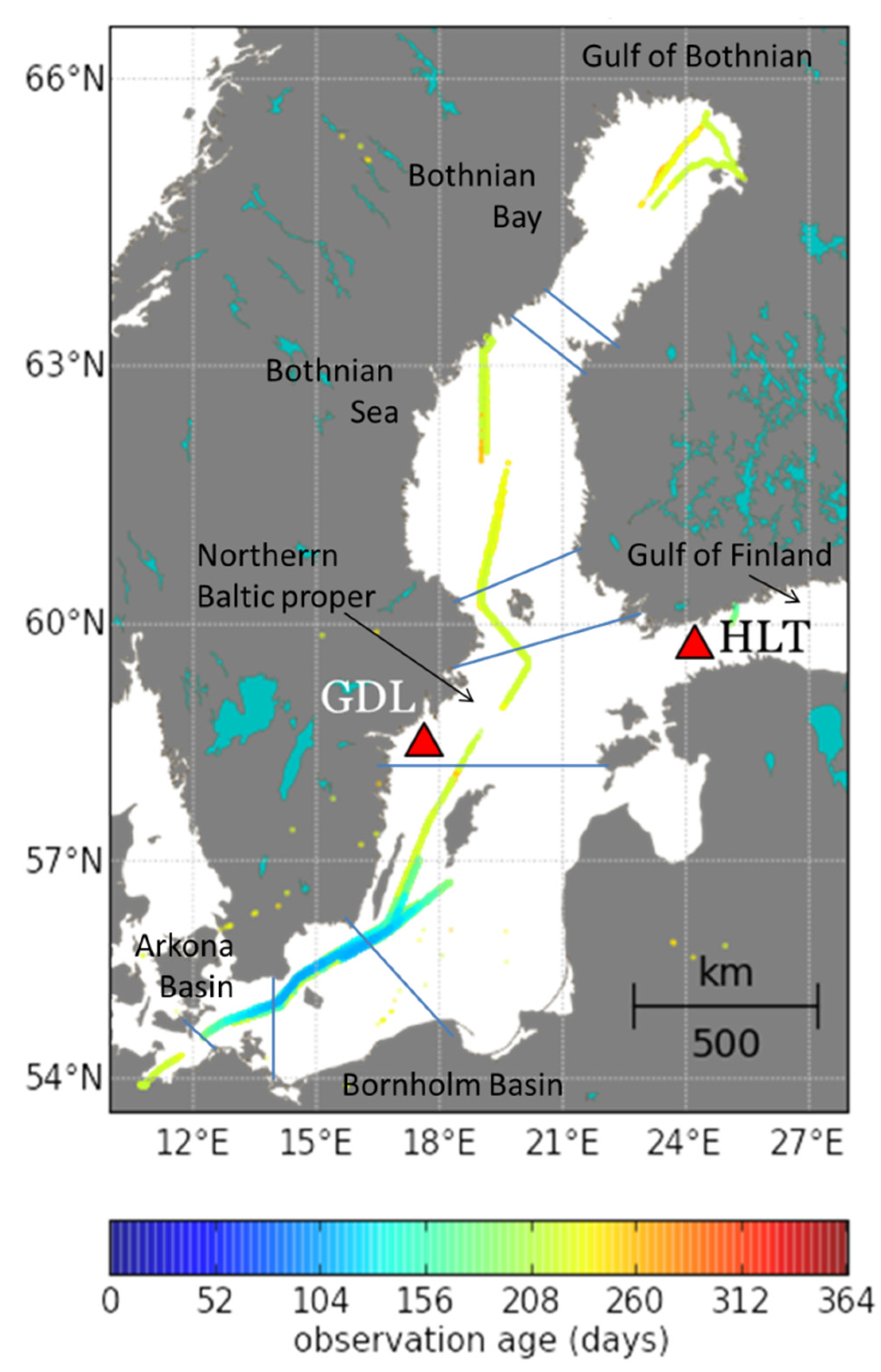
2.1. In Situ Radiometric Data

The assessment of OLCI-A, VIIRS and MODIS-Aqua R r s products was undertaken using data from AERONET-OC and Alg@line from April 2016 to September 2018 (Figure 1). The two AERONET-OC sites are the Gustaf Dalén Lighthouse Tower (GDL) in the northern Baltic Proper established in 2005 and the Helsinki Lighthouse Tower (HLT) in the Gulf of Finland established in 2006, for which the sensors, platforms and data processing are described in detail in Zibordi et al. [28,29]. Since 2018, the deployment of CE-318T 12-channel radiometer systems within the AERONET-OC network provides additional spectral bands centred at 400, 510, 620 and 779 nm for marine water sites and 681 and 709 nm at inland water sites [29]. The CE-318T systems also increased the frequency of measurement sequences from 30 min to 5 min to provide a finer temporal scale resolution to detect environmental perturbations [29]. For the GDL and HLT data in this study, the CE-318 9-channel radiometer systems were used, which measures at the spectral bands corresponding to MODIS-Aqua and VIIRS. AERONET-OC Level 2.0 data at GDL and HLT were obtained from http://aeronet.gsfc.nasa.gov (accessed on 24 October 2021). The AERONET-OC waveband centres are 412, 439, 500, 554, 675 and 870 nm for the GDL and 413, 441, 491, 555, 668 and 870 nm for the HLT. To match with the spectral bands of OLCI-A, MODIS-Aqua and VIIRS, water-leaving radiance corrected for viewing angle dependence and the effects of the non-isotropic distribution of the in-water radiance field ( L w N -f/Q) were band-shift corrected following Zibordi et al. [28], based on a regional bio-optical algorithm to reduce inter-band uncertainties. The corresponding R r s were computed from the band-shifted L w N -f/Q data using the extra-atmospheric solar irradiance ( F 0 ) for each waveband as in Qin et al. [30] and including the NIR band at 709 nm, which was linearly interpolated from the 665 nm band.
The Alg@line data set is described in [31] and the methods for processing shipborne data are described in detail in [30]. In brief, the system consists of three RAMSES spectro-radiometers (TriOS, Rastede, Germany) mounted near the bow of the ferries M/S Finmaid and Transpaper. The azimuth angle of the instruments was kept as close to 135° and always > 90°, using a stepper motor platform with GPS time and location to compensate for the vessel heading [32]. The fingerprint method was used to determine the reflectance of sky radiance at the air–water interface (ρs) [32,33]. To eliminate spurious observations, the data underwent a rigorous screening procedure based on assumptions of the spectral shapes of reflectance in these highly absorbing and weakly scattering waters [30]. For these waters, we are also interested in the performance of OLCI in the NIR, which can be used in band ratios to estimate the Chl a concentration [16]. It is generally assumed in waters with low particle scattering that NIR reflectance is close to zero [34]. This assumption generally holds in the Baltic Sea outside peak productivity periods or close to rivers and shallow areas, when there can be higher concentrations of phytoplankton, detrital material or sediment in surface waters. Additionally, residual surface water effects such as spray, sun glint and whitecaps will elevate R r s in the visible and NIR. Individual spectra were inspected to evaluate the shape of the NIR signal for signs of high particle scattering. When no elevated particle scattering was observed, as evidenced by a spectrally flat NIR signal, any offset observed in the NIR was assumed to be caused by spectrally neutral effects and corrected for by subtracting the mean R r s ( 850 900 ) from the entire spectrum [30].

2.2. OLCI-A, VIIRS and MODIS-Aqua Processors

OLCI-A full-resolution data L1B and L2 products were downloaded from the EUMETSAT Data Centre and Copernicus Online Data Access (CODA) portals respectively. OLCI-A processing baseline (pb) 2.23–2.29 is described in [35] and the associated Algorithm Theoretical Baseline Document (https://www.eumetsat.int/ocean-colour-resources (accessed on 24 October 2021)). The AC for pb OL_L2M.003.00 is described in collection report 3 (https://www.eumetsat.int/media/47794 (accessed on 24 October 2021)) and includes updates to system vicarious calibration gains, bright pixel correction, cloud masking [36], flags and whitecap correction [37,38].
The coupled ocean–atmosphere algorithm POLYMER v4.13 models the contribution to TOA reflectance as a polynomial and a forward bio-optical model is used for the water component [39]. The coastal aerosol model C2R-CC [40] uses coastal AERONET-OC measurements [41], and a parameterised version of the successive order of scattering technique to compute the atmospheric radiative transfer [42], which is implemented as a neural network (NN) regression. The latest NASA Ocean Colour Reprocessing (R2018.0) for MODIS-Aqua and Suomi-VIIRS were used. Each of the AC processors applied to OLCI-A data uses a different system vicarious calibration (SVC). The OLCI pb 2.23–2.29 uses a climatological SVC [43] whereas OL_L2M.003.00, MODIS-Aqua and VIIRS implement SVC based on match-ups with MOBY. POLYMER uses an in situ based SVC designed for ocean–atmosphere coupled algorithms [44]. In order to exclude unreliable satellite measurements for each product, a set of recommended quality flags for each AC processor (Table 1) were applied as a mask to each pass.

2.3. Match-Up Procedure and Statistics

The method used for match-up analysis follows [45], and was adapted for high-frequency data following [46]. Satellite over-passes were within ±1 h of the in situ Alg@line and AERONET-OC measurements. The in situ data (1 min bins) were matched to individual satellite pixels. From the 3 × 3 pixels, the centre pixel was used for the validation procedure. All in situ data within a specific pixel were averaged, so that each matchup has an independent set of in situ data and there was no overlapping in situ data between match-ups. The validation statistics were computed on the centre pixel, to ensure that each matchup uses an independent satellite pixel. Additionally, the standard deviation around the matchup (from the 3 × 3 box) was computed as an index of the homogeneity of the matchup. The number of granules for each sensor was 38 for OLCI-A, 40 for VIIRS and 7 for MODIS-Aqua. The minimum distance between match-ups in the satellite image is reflected in the resolution of each sensor which for OLCI-A is 300 m, MODIS-Aqua is 1 km and VIIRS is 750 m. The satellite data were extracted from a 3 × 3-pixel box centred on the in situ observations and were excluded if the median coefficient of variation (CV) was >0.15 (from 412 to 555 nm) or when <50% of pixels were valid [45]. The CV criterion also removed data within 5 min of the satellite overpass, which contained the ship in one of the pixels. The following statistical metrics were used to evaluate algorithm performance following [47,48]: type-II regression slope (S), intercept (I), Pearson correlation coefficient (r), root-mean-square difference (RMSD—Ψ), the bias (δ), bias-corrected root-mean-square error (Δ) and the relative percentage difference (RPD).

3. Results

The hyperspectral R r s from the shipborne measurements covered a wide range of signal amplitudes, varying from <0.002 sr−1 at 560 nm during April, to >0.01 sr−1 in June and August (Figure 2). The change in R r s spectral shape reflected the seasonal variability in these highly absorbing, weakly scattering waters. In April and May, the low signal and flattening of the R r s   spectra is a consequence of the Chl a and aCDOM concentrations during spring. The more prominent R r s peak at 560 nm during June to August corresponds to the period of summer phytoplankton blooms when the largest number of R r s spectra were available. The radiometric assessment of satellite products is therefore weighted towards late spring and summer, with the shipborne observations observing a wider variety of phytoplankton blooms and degrees of vertical mixing (thermal stratification is common in summer). The matchup procedure led to N = 208 in situ R r s coincident with OLCI-A pb2, OL_L2M.003.00, C2R-CC and POLYMER (N = 199 for Alg@line, N = 9 for AERONET-OC), 475 with Suomi-VIIRS (N = 429 for Alg@line, N = 46 for AERONET-OC) and 177 (N = 122 for Alg@line, N = 45 for AERONET-OC) with MODIS-Aqua (Table 2, Figure 3 and Figure 4). The AERONET-OC data consistently had lower R r s (λ) values than the Alg@line data (Figure 3), reflecting differences in biogeochemical water constituents between the coastal AERONET-OC sites and the wider range of environmental conditions encountered along the deeper water Alg@line ferry transects (Figure 1). OLCI-A pb 2.23–2.29, OL_L2M.003.00 and Suomi-VIIRS tended to underestimate R r s   at all visible bands. The spectral shape of R r s for these processors were similar in the green and red to in situ R r s , with some spectral differences in the blue with either an uncharacteristic peak at 412 nm or negative values (Figure 3).
For OLCI-A pb 2.23–2.29 at 412 and 443 nm, there was a consistent underestimate at low values <0.001 sr−1 corresponding to both in situ AERONET-OC and Alg@line R r s and an overestimate at values >0.0015 sr−1 corresponding to the in situ Alg@line data only (Figure 4). At 560 nm with an increase in the R r s   signal, pb 2.23–2.29 performed better, and had zero δ, but high Ψ and Δ, indicative of the high scatter that can be seen in Figure 4. At 665 and 709 nm, Ψ and Δ were lower but δ increased, caused by the tendency to underestimate R r s at at these bands (Figure 4), which is reflected in the negative I and δ (Table 2). Generally the scatter around the 1:1 for OL_L2M.003.00 was similar to pb 2.23–2.29, but the offset from the 1:1 was greater (Figure 4), especially at 412 and 443 nm, which resulted in the largest S, I, Ψ and Δ and smallest r of all the AC processors. At 412 nm and 443 nm, the RPD for OL_L2M.003.00 was ~92 and 60%, respectively, which is the highest of all of the ACs evaluated. Similarly, for OL_L2M.003.00 at R r s (674) and R r s (709), the S was the lowest of all the AC processors (Table 2).
The closest match to in situ R r s   from both AERONET-OC and Alg@line was OLCI-A POLYMER, (Figure 3), which at 412, 442, 560, 665 and 709 nm was within 30% (Table 3). POLYMER also had the highest r, which is indicative of linear consistency between the in situ and satellite data (Figure 5). At R r s (412), OLCI-A POLYMER consistently outperformed the other ACs having the lowest Ψ, δ and Δ, which indicate low scatter around the 1:1, few outliers and no systematic bias, respectively (Table 3). OLCI-A POLYMER also had the lowest δ at R r s (490) and R r s (665), which is reflected in the tight fit and proximity of the points to the 1:1 (Figure 5). For all bands, there was an underestimate at high R r s values, which resulted in a low S, however (Table 3, Figure 5). POLYMER also exhibited an uncharacteristic peak in the red towards 700 nm (Figure 3). C2R-CC tended to overestimate R r s   at all bands (Figure 5), and exhibited artefacts in the blue often with another peak at 490 nm, which does not correspond to either of the in situ datasets, plus it had a high offset from zero across the spectrum (Figure 3). This gave rise to the high S, I and Ψ and low r at blue and blue-green bands resulting in RPD of between 66 and 80% (Table 3). The performance of C2R-CC improved at 560, 665 and 709 nm, and the S and r were closer to 1 and I, Ψ, δ and Δ were all lower and the RPD was between −1 and 37% (Table 3). At 560, 665 and 709 nm, even though the Ψ and Δ were higher or similar for C2R-CC compared to POLYMER, the S were closer to the 1:1 and I were lower (Table 3).
Suomi-VIIRS returned the highest number of match-ups with R r s (λ) values covering a higher range than the other ACs (Figure 6), but exhibited a consistent underestimate as indicated by the comparatively high Ψ, δ and Δ (Table 4), especially at higher R r s values. The RPD for VIIRS varied from 22% at 560 nm to 38% at 671 nm and 67% at 412 nm (Table 4). For MODIS-Aqua the spectra reproduced the shape of the in situ AERONET-OC data well, but not for the Alg@line data (Figure 6). MODIS-Aqua both overestimated and underestimated R r s (412) and R r s (443), as conveyed by the high S, I and RPD (Table 4). MODIS-Aqua performed better at 488, 560 and 667 nm with comparatively low I, Ψ, δ and Δ and S close to 1, especially at 560 and 667 nm (Table 4).
Composite ocean colour satellite images from OLCI-A using the four ACs, MODIS-Aqua and VIIRS for the Baltic Sea at 560 nm were processed for the period from 11 to 17 June 2016 (Figure 7). OLCI-A C2R-CC returned the highest R r s (560) followed by POLYMER and OL_L2M.003.00, especially in the southern Baltic Sea. C2R-CC also provided the greatest pixel coverage over the whole area during this period, whereas pb 2-23-2029 and OL_LM.0003.00 had the lowest coverage (Figure 7), presumably due to differences in the cloud mask flags. The MODIS-Aqua image had the lowest R r s (560). For each processor, data were extracted for R r s (443), R r s (560) and R r s (665) at every 20 km from north–south and east–west transects (shown as red lines on pb 2.23-2.29 image in Figure 7), to compare the different ACs over large spatial areas of the Baltic Sea. The pattern was the same for each waveband and transect: OLCI-A POLYMER and OL_L2M.003.00 were closest to the in situ R r s ferry data, whereas OL_L2M.003.00, MODIS-Aqua and VIIRS were closest to in situ AERONET-OC R r s . C2R-CC consistently returned the highest values, especially for R r s (443) in the southern part of the transect and for R r s (665) in the northern part of the transect. OLCI-A pb 2 and OL_L2M.003.00 had the lowest R r s along both transects and especially at R r s (443) for OLCI-A pb 2. MODIS-Aqua and VIIRS were similar and generally lower than OLCI-A POLYMER. The exception to this was for POLYMER R r s (665) that had a cluster of points at the northern-most part of the north-south transect which were lower than the in situ R r s (665).

4. Discussion

From the dawn of SeaWiFS through the maturing ocean colour age of MODIS-Aqua and MERIS, these satellite sensors have provided accurate Chl a retrieval in open-ocean, shelf-seas and many coastal environments for the past two decades [49,50]. Regions with high CDOM however, pose a particular challenge due to low signal amplitude with overlapping absorption signatures of CDOM and Chl a [51]. In the Baltic Sea, previous studies showed that SeaWiFS and MODIS-Aqua underestimated L W N in the blue and red and that the uncertainties and bias were high [52], potentially resulting in an overestimate in Chl a. This is due to the low L W N signal under the influence of high CDOM and an overestimate in the aerosol optical depth. AC models need to capture and reproduce this large variation in both atmospheric and oceanic conditions.
The atmospheric masses over the region are influenced by both land and marine aerosols, which are highly variable. In the central part of the Baltic Sea, the average aerosol optical thickness is 1.3 [53]. The burning of agricultural straw in northern Europe and Russia during April is thought to increase the aerosol optical thickness [54]. The surface water inherent optical properties of the Baltic Sea are dominated by CDOM with the secondary, seasonal spring–summer influence of phytoplankton [54]. The variability in the surface water conditions is reflected in the spectral shape of the in situ R r s (λ), with the high CDOM causing a flattening of the spectra at 412 nm (Figure 2), low values at 443 nm, a high peak at 560 nm indicative of the spring bloom and a smaller peak at 709 nm due to a higher backscatter from small particles, such as cyanobacteria or TSM (Figure 2). Spring bloom Chl a in the Baltic Sea can be as high as 10 to 120 mg m−3 whereas during summer the range in Chl a is typically 1 to 3 mg m−3, but can increase to between 5 and 30 mg m−3 in July and August when cyanobacteria bloom [24]. Some estuarine locations around the Baltic Sea can be influenced by TSM [54]. The variability in CDOM and TSM at river mouths is expected to decrease R r s (λ) at blue and blue-green bands as TSM and the ratio of backscatter to absorption increases, which would produce a higher slope in the R r s (λ) spectra from the blue to the green. An increase in TSM loads and therefore backscatter would also be observed in an increase in the offset in R r s (λ) in the NIR (Figure 2). For the match-ups in this study, the ferry tracks mostly traverse the deeper waters of the Baltic Sea and the AERONET-OC sites are located away from major rivers (Figure 1). The AERONET-OC sites are located in the northern Baltic Proper and the Gulf of Finland where a C D O M (412) can be between 0.8 to 1.6 m−1 [55]. The AERNOT-OC R r s (λ) provided 4% of the total match-ups with OLCI-A, 10% with VIIRS and 31% with MODIS-Aqua (Table 2, Table 3 and Table 4). The lower R r s (λ) in the blue and green at the AERONET-OC stations especially at the HLT (Figure 3a,b), mirrors the high absorption by CDOM and low scattering at these sites [12,56]. The riverine input of CDOM is particularly high in the eastern Gulf of Finland [11,12,57], and follows a dilution gradient towards the northern Baltic Proper, with the HLT located approximately halfway. The highest a C D O M (412) in the Baltic Sea can be found further east in the Gulf of Finland, towards St Petersburg in Neva Bay (not shown in Figure 1), where values are generally >2.5 m−1 and can reach 15 m−1 [11,12].
The objective of deploying autonomous measurement systems on the ferries was to provide more R r s (λ) data at other sites, to be able to capture the variability in both atmospheric and water conditions from Bothnian Bay in the north to the Bornholm Basin in the south (Figure 1). The ferry data provided the largest number of match-ups with the ocean colour sensors that were assessed (Table 2, Table 3 and Table 4). Most of the match-ups were between 54 and 56° N in the Arkona and Bornholm basins (Figure 1), where a C D O M (412) is typically between 0.4 and 1.1 m−1. In the deeper water, observed during the day-lit part of the Alg@line stations, the R r s (λ) signal in the green was far higher (Figure 3b), while the number of observations collected here was relatively small. Towards the southern Baltic Sea a C D O M (412) is lower (<0.6 m−1) while TSM and the associated scattering increase, causing a pronounced increase in R r s (560) [54]. There are large areas in the central part of the Baltic Sea where a C D O M (412) remains fairly homogeneous [56]. In the north in the Gulf of Bothnia, a C D O M (412) can be >1.8 m−1 [54,56], which correspond with the lowest R r s (λ) in the Alg@line data (Figure 3b). Towards the southern Baltic Sea a C D O M (412) is lower (<0.6 m−1) while Chl a and the associated scattering increases which causes a pronounced increase in R r s (560) [54] as seen in Figure 3b.
The precursor ocean colour satellite sensor to OLCI was MERIS, which had similar bands and characteristics. At the two AERONET-OC sites in the Baltic Sea, Zibordi et al. [27] reported differences of +15 to +42% for MERIS over the spectral range 443 to 555 nm compared to SeaPRISM L W N (N = 41). Using an updated version of the MERIS AC MEGS L W N product, Zibordi et al. [52] subsequently reported (N = 12 to 39) that the accuracy at 490, 560 and 665 nm was improved (ψ < 24%). Some studies reported that C2R-CC improved the performance of MERIS R r s [19,23,24]. For OLCI-A pb 2 in the Baltic Sea at the AERONET-OC sites (N = 42), Zibordi et al. [7] reported an underestimation in L W N at blue spectral bands due to an overestimate in the aerosol optical depth at 865 nm. In this study, we also observed underestimation by OLCI-A pb 2 in the blue at low R r s (λ) and an overestimate at the higher range of values (Figure 4). The updated OL_L2M.003.00 has been found to be more accurate than OLCI-A pb 2 in the oligotrophic waters of the Atlantic Ocean [3]. In the Baltic Sea, the OL_L2M.003.00 product underestimated R r s (λ) in the blue especially at low values, and also overestimated R r s (λ) in the green, red and NIR at the higher range of values (Figure 4), which resulted in a low linear regression S and an increase in the RPD (Table 2). OL_L2M.003.00 was therefore less accurate than OLCI-A pb 2 for the Baltic Sea. The OL_L2M.003.00 processing applies new system vicarious calibration gains based on the standard OC methodology [57], there has been an update to the bright pixel correction removing any residual water reflectance in the NIR, a spectrally resolved white cap correction has been applied which should improve the quality of the product at wind speeds between 6.3 and 12 ms−1 and an update to the cloud flags to remove potential pixels contaminated by clouds (https://www.eumetsat.int/media/47794 (accessed on 24 October 2021)). The poor performance of OL_L2M.003.00 for the Baltic Sea region is possibly due to difficulties with the AC in reproducing correctly the signal from the atmosphere and the highly absorbing water when R r s (λ) (particularly in the blue) is so low, the aerosol model library not being optimal for these waters and that bright pixel scheme implemented does not converge properly, which caused the underestimate in the NIR (Figure 4). Assessing other AC processors for OLCI-A, we found that POLYMER is the most accurate with differences of 22, 17 and 28% at 443, 560 and 665 nm, respectively (N = 208). Similarly, off the south-east Canadian coast, where aCDOM(442) can reach 4 m−1, OLCI-A POLYMER has also been found to be the most accurate AC [4]. Alikas et al. [25] also found that POLYMER is the most accurate AC for the Baltic Sea and Estonian Lakes, but the difference was 57% at blue wavebands skewed by the data from the Lakeds. The superior performance of the version of POLYMER developed for OLCI in the Baltic Sea is probably due to (i) the polynomial atmospheric model reproduces well the scattering and absorption by the atmosphere under both sun glint and thin cloud conditions [39,58]; (ii) the quality of the atmospheric signal at high latitudes has been improved [44]; (iii) since the version of POLYMER developed for MERIS, there have also been updates to the water reflectance model for the derivation of both Chl a and the backscattering signal in both case 1 and 2 waters which also include bidirectional effects [44]. For the Baltic Sea, this may be somewhat surprising since the OLCI version of POLYMER has been calibrated more for Chl a and TSM dominated waters and is expected to perform less well in areas dominated by CDOM [4,44]. From the dispersion of the points at higher R r s (λ) values in the blue and the resulting low S, clearly improvements in OLCI-A POLYMER are required for the Baltic Sea region. Overall the results for OLCI-A POLYMER are encouraging and imply that this AC could also be accurate in regions with similar IOPs and range in a C D O M (λ) such as the Amazon River plume ( a C D O M (355) 0.3–2.5 m−1) [59], the Black Sea ( a C D O M (325) 0.4–1.4 m−1) [60], Bohai, east China and Yellow Seas ( a C D O M (355) 0.2–1.2 m−1) [61].
C2R-CC exhibited the worst performance for the Baltic Sea at blue and green bands, which were >65% at 412, 443 and 490 nm and >35% at 560 nm. Accounting for uncertainties in the in situ R r s in the Baltic Sea, Alikas et al. [25] also found that the OLCI-A C2R-CC processor exhibits a large difference (~107%) compared to in situ R r s (N = 15). For OLCI-A, two studies in the Baltic found that the previous version of C2R-CC performed well in retrieving the R r s spectral shape (N = 29) [26,62]. In this study, the performance of C2R-CC improved from the green to red to NIR, with an S closer to the 1:1, though the scatter was still relatively high (Figure 4). This may suggest that C2R-CC could produce accurate Chl a values for the region when using red: NIR R r s (λ) band ratio algorithms. The calibration of the C2R-CC requires sufficient data to account for the effects of different aerosol types, cirrus clouds, sun and sky radiance, and the coupling between them and the air molecules [62]. Improvements to the C2R-CC have been made to both the atmospheric and in-water NNs, and for the water component, this includes a more extensive training range, which for aCDOM(442) is now from 0.001 to 22 m−1 (https://www.eumetsat.int/media/47794 (accessed on 24 October 2021)). There are two possible reasons why the C2R-CC does not perform well in blue bands for the Baltic Sea. The first is probably due to none convergent or optimal solutions caused by the in-water NN, as has been observed in other studies using different ocean colour sensors [30,63]. For MERIS, it was found that adding further training data could lead to ‘overtraining’ by offering multiple solutions to retrieve R r s or IOPs, which may not necessarily result in accurate R r s [63]. The second reason is that the calibration data used in the atmospheric NN still does not cover the variability in atmospheric conditions that occur over the Baltic Sea
Previous studies on MODIS-Aqua L W N at Baltic Sea AERONET-OC sites reported large uncertainties (~60%) and biases (~20%) at blue bands and an overestimate in τa at 869 nm of ~95%, indicative of errors in the AC aerosol model [18]. Extension of the aerosol model for MODIS-Aqua to include α values to 1.7 has been recommended [18], especially to capture the range in mixed continental-industrial type aerosols in summer [64]. The AC developed for MODIS-Aqua and VIIRS [65,66] applies a NIR correction that accounts for particle backscattering based on a variable slope plus an estimate for absorption at red and NIR bands [67]. There is often a negative bias across all wavelengths, which for MODIS-Aqua is most pronounced in the blue [50]. In highly absorbing waters, MODIS-Aqua can exhibit very high relative uncertainty at blue bands (up to 60%) where strong absorption makes the signal low, and in the red (up to 40%) where the signal is also low due to strong water absorption [50]. In the green, the uncertainty for MODIS-Aqua is ~20% [50]. For the Baltic Sea specifically, Goyens et al. [68] reported that the relative error for MODIS-Aqua at 412 nm was 55%, at 547 nm was 15% and at 667 nm was 25%. Similarly, our data indicated a small negative bias across all wavelengths except 412 nm and that the RPD was even higher in the blue (~84% at 412 nm) and within the range reported by Moore et al. [50] for green (~16% at 560 nm) and red bands (~33% at 667 nm). The cause of the negative bias is attributed to L w being non-zero in the NIR which results in an overestimation of the aerosol optical thickness and an underestimation in L w [69], which when extrapolated from the NIR across the bands, the error is greater in the blue [50]. Above coastal waters, light-absorbing aerosols can also contribute to the negative bias in L w . In the Baltic Sea, the negative bias in MODIS-Aqua R r s is due to a systematic underestimation in the Ångström coefficient and an overestimation of the optical thickness [68]. An overestimate in MODIS-Aqua aerosol optical thickness of 101% at the GDL and 91% at the HLT has been reported [69]. Due to these errors in the standard MODIS-Aqua AC, a multilayer neural network (MLNN) AC method for MODIS-Aqua was subsequently developed and compared with the SeaDAS NIR and NIR/SWIR algorithms and a C2R-CC version for MODIS-Aqua [70]. For the Baltic Sea, the MLNN algorithm reduced the L W N   APD by more than 60% for blue bands compared to the standard SeaDAS AC. In our study, using the latest reprocessing (R2018) for MODIS-Aqua (N = 177 match-ups) and VIIRS (N = 475), the RPD at 443 nm was 34% for both sensors and was 17% for MODIS-Aqua and 22% for VIIRS at 560 nm, but at 667 nm the RPD increased to 33 and 38%, respectively.
As discussed above, the AERONET-OC and Alg@line data are located in different environments; both being predominantly influenced by CDOM, which is generally higher at the AERONET-OC sites, whereas the Alg@line tracks pick up a stronger signal from spring–summer phytoplankton blooms. Some trends in the validation plots for the different ACs may also partly arise from differences in data sources between the in situ AERONET-OC and Alg@line R r s due to the nature of the sites, quality and processing of the data. The uncertainty of the TriOS-RAMSES system is greater in the blue (>6%) than in the green (3.5%) and red (4.5%), compared with CIMEL-SeaPRISM which has uncertainties of 4.5, 4 and 10%, respectively [71]. The TriOS-RAMSES radiometers deployed on Alg@line have been inter-compared with CIMEL-SeaPRISM at the stable AERONET-OC platform of the Aqua Alta Oceanographic Tower. The differences between TriOS-RAMSES and CIMEL-SeaPRISM were 8% difference at 443 nm, 6% at 555 nm and 10% at 667 nm [72]. Future studies should evaluate differences between the sensors using a common processor and for the TriOS-RAMSES, the sun-tracker stepper motor used in this study. There is one caveat, that the methodology for calculating E d and subsequent optimisation of R r s are not directly comparable between AERONET-AC and the automated TriOS-RAMSES (plus the fingerprint method), although both have been used in combination in previous studies without showing major biases [30,34].
Ocean colour is an Essential Climate Variable [73,74], the study of which requires long time-series data to assess climate-induced changes in phytoplankton. To this end, there have been a number of initiatives to merge multi-mission datasets [75,76]. The starting point for this is the best AC performance for a single sensor followed by the application of the R r s product to multi-mission data, computation of Chl a and analysis of reproducibility of patterns in the Chl a time series for a single sensor in the multi-mission data [77]. For this, the AC model needs to be as accurate as possible and have the largest number of data points in both space and time. In this study, we found that the consistency between different OLCI-A, MODIS-Aqua and VIIRS AC products was poor. We performed a comprehensive analysis of AC processors for OLCI-A, which showed that POLYMER is the most accurate over all bands and provides the largest number of complete and consistent data points for Baltic Sea images. The performances of Suomi-VIIRS in the blue, and OLCI-A C2RCC and MODIS-Aqua in the red and NIR were also good. For the Baltic Sea, there is growing consensus that POLYMER for OLCI-A [25] is the most accurate AC. Future studies should evaluate the performance of MODIS-Aqua and VIIRS with POLYMER and evaluate if it is the most accurate AC for generating ocean colour time series from multiple-satellite missions. The POLYMER AC may improve the consistency between OLCI-A, MODIS-Aqua and VIIRS.

5. Conclusions

The performance of four AC processors (pb 2, OL_L2M.003.00, C2R-CC and POLYMER) for OLCI-A and standard processors for MODIS-Aqua and VIIRS were assessed in the Baltic Sea using in situ R r s from AERONET-OC and ferries. OLCI-A with POLYMER performed well at 412, 442 and 560 nm with ψ <30% and a δ of between −0.0001 and −0.0004, but all bands exhibited an underestimate as R r s values increased. The other OLCI-A AC processors showed relatively poor performance in the blue (412 and 443 nm), red and NIR wavebands, but better performances at 560 nm where the signal was highest. Of the OLCI-A processors, C2R-CC exhibited the worst performance in the blue, and generally, ψ was >30% for all wavebands but showed better performance at 665 and 709 nm. VIIRS underestimated R r s across all bands, which was notably large at 412 nm, where the differences with in situ R r s were >65%, and also especially at higher R r s values in green and red bands. MODIS-Aqua was more accurate in the blue-green to red bands compared to the blue, especially R r s (412) which had a difference of ~85% compared to in situ R r s . Of the OLCI AC processors tested, the results suggest that OLCI POLYMER will generate the most accurate biogeochemical monitoring water quality parameters, though improvements in this AC are still required for the Baltic Sea.

Author Contributions

Conceptualisation, G.H.T. and S.G.H.S.; methodology, G.H.T., S.G.H.S., S.P. and P.Q.; software, S.P. and N.S.; validation, S.P., G.H.T., S.G.H.S. and N.S.; formal analysis, S.P., G.H.T., P.Q., D.D., N.S. and E.K.; investigation, G.H.T., S.P., S.G.H.S. and E.K.; resources, G.H.T. and S.G.H.S.; data curation, S.G.H.S., S.P., P.Q., N.S., D.D. and E.K.; writing—original draft preparation, G.H.T., S.P. and S.G.H.S.; writing—review and editing, G.H.T., S.P., S.G.H.S. and E.K.; visualisation, S.P., P.Q. and S.G.H.S.; supervision, G.H.T., S.G.H.S. and E.K.; project administration, G.H.T., S.G.H.S. and E.K.; funding acquisition, G.H.T. and S.G.H.S. All authors have read and agreed to the published version of the manuscript.

Funding

GT and SPA were supported by S3-EUROHAB (Sentinel-3 products for detecting EUtROphication and Harmful Algal Bloom events) from the European Regional Development Fund through the INTERREG France-Channel-England, as part of the assessment of transferability of the project outputs. PQ was funded by a scholarship from the Chinese Scholarship Program. SS and NS received funding from the European Union’s Horizon 2020 research and innovation programme under grant agreement No 776480 (MONOCLE).

Data Availability Statement

The satellite and in situ R r s data from April 2016 to September 2018 for the Baltic Sea used in the study are freely available at the following repositories: For Sentinel-3 OLCI-A pb 2 from https://eoportal.eumetsat.int/ (accessed on 24 October 2021); OLCI-A OL_L2M.003.00 from https://rsg.pml.ac.uk/shared_files/PB3_BAL (accessed on 24 October 2021); OLCI-A C2R-CC from https://rsg.pml.ac.uk/shared_files/C2RCC_BAL (accessed on 24 October 2021); OLCI-A POLYMER from https://rsg.pml.ac.uk/shared_files/POLYMER_BAL (accessed on 24 October 2021); NASA MODIS-Aqua (R2018) from https://oceandata.sci.gsfc.nasa.gov/directaccess/MODIS-Aqua/L2/ (accessed on 24 October 2021); NASA Suomi-NPP VIIRS data (R2018) from https://oceandata.sci.gsfc.nasa.gov/directaccess/VIIRS-SNPP/L2/ (accessed on 24 October 2021); AERONET-OC from http://aeronet.gsfc.nasa.gov (accessed on 24 October 2021); and Alg@line data can be downloaded via https://doi.org/10.5281/zenodo.5572537 (accessed on 24 October 2021).

Acknowledgments

The authors thank the captain and crews of M/S Finmaid (Finnlines) and Transpaper (TransAtlantic); Giuseppe Zibordi from the Joint Research Center for AERONET-OC data and for Reviewer comments that significantly improved the paper; the Natural Environment Research Council Earth Observation Data Acquisition and Analysis Service (NEODAAS) for acquisition of satellite imagery and the computing cluster to process them.

Conflicts of Interest

The authors declare no conflict of interest.

References

  1. Donlon, C.; Berruti, B.; Buongiorno, A.; Ferreira, M.H.; Femenias, P.; Frerick, J.; Goryl, P.; Klein, U.; Laur, H.; Mavrocordatos, C.; et al. The global monitoring for environment and security (GMES) sentinel-3 mission. Remote Sens.Environ. 2012, 120, 37–57. [Google Scholar] [CrossRef]
  2. Zibordi, G.; Talone, M.; Voss, K.J.; Johnson, C.B. Impact of spectral resolution of in situ ocean color radiometric data in satellite matchups analyses. Opt. Express 2017, 25, A798–A812. [Google Scholar] [CrossRef] [PubMed] [Green Version]
  3. Tilstone, G.H.; Pardo, S.; Dall’Olmo, G.; Brewin, R.J.W.; Nencioli, F.; Dessailly, D.; Kwiatkowska, E.; Casal, T.; Donlon, C. Performance of ocean colour algorithms for Sentinel-3 OLCI, MODIS-Aqua and VIIRS in open-ocean waters of the Atlantic. Remote Sens. Environ. 2021, 260, 112444. [Google Scholar] [CrossRef]
  4. Giannini, F.; Hunt, B.P.V.; Jacoby, D.; Costa, M. Performance of OLCI Sentinel-3A satellite in the Northeast Pacific coastal waters. Remote Sens. Environ. 2021, 256, 112317. [Google Scholar] [CrossRef]
  5. Li, J.; Jamet, C.; Zhu, J.H.; Han, B.; Li, T.J.; Yang, A.N.; Guo, K.; Jia, D. Error budget in the validation of radiometric products derived from OLCI around the China Sea from open Ocean to Coastal Waters Compared with MODIS and VIIRS. Remote Sens. 2019, 11, 2400. [Google Scholar] [CrossRef] [Green Version]
  6. Mograne, M.A.; Jamet, C.; Loisel, H.; Vantrepotte, V.; Meriaux, X.; Cauvin, A. Evaluation of five atmospheric correction algorithms over French optically-complex waters for the Sentinel-3A OLCI Ocean Color Sensor. Remote Sens. 2019, 11, 668. [Google Scholar] [CrossRef] [Green Version]
  7. Zibordi, G.; Mélin, F.; Berthon, J.F. A Regional Assessment of OLCI Data Products. IEEE Geosci. Remote Sens. Lett. 2018, 15, 1490–1494. [Google Scholar] [CrossRef]
  8. Renosh, P.R.; Doxaran, D.; Keukelaere, L.D.; Gossn, J.I. Evaluation of atmospheric correction algorithms for sentinel-2-MSI and sentinel-3-OLCI in highly turbid estuarine waters. Remote Sens. 2020, 12, 1285. [Google Scholar] [CrossRef] [Green Version]
  9. Leppäranta, M.; Myrberg, K. Physical Oceanography of the Baltic Sea; Springer Science & Business Media: Berlin/Heidelberg, Germany, 2009. [Google Scholar]
  10. Omstedt, A.; Elken, J.; Lehmann, A.; Piechura, J. Knowledge of the Baltic Sea physics gained during the BALTEX and related programmes. Prog. Oceanogr. 2004, 63, 1–28. [Google Scholar] [CrossRef]
  11. Woźniak, M.; Bradtke, K.M.; Krężel, A. Comparison of satellite chlorophyll a algorithms for the Baltic Sea. J. Appl. Remote Sens. 2014, 8, 083605. [Google Scholar] [CrossRef] [Green Version]
  12. Ylöstalo, P.; Seppälä, J.; Kaitala, S.; Maunula, P.; Simis, S. Loadings of dissolved organic matter and nutrients from the Neva River into the Gulf of Finland–Biogeochemical composition and spatial distribution within the salinity gradient. Marine Chem. 2016, 186, 58–71. [Google Scholar] [CrossRef]
  13. IOCCG Atmospheric Correction for Remotely-Sensed Ocean-Colour Products. In Technical Report: Reports of the International Ocean-Colour Coordinating Group; Wang, M. (Ed.) International Ocean-Colour Coordinating Group: Dartmouth, NS, Canada, 2010; Volume 10, Available online: https://www.ioccg.org/reports/report10.pdf (accessed on 24 October 2021).
  14. Koponen, S.; Attila, J.; Pulliainen, J.; Kallio, K.; Pyhälahti, T.; Lindfors, A.; Rasmus, K.; Hallikainen, M. A case study of airborne and satellite remote sensing of a spring bloom event in the Gulf of Finland. Cont. Shelf Res. 2007, 27, 228–244. [Google Scholar] [CrossRef]
  15. Krawczyk, H.; Neumann, A.; Walzel, T.; Hetscher, M.; Siegel, H. Application of multispectral interpretation algorithm to remote sensing data over the Baltic Sea. In Proceedings of the Ocean Optics XIII, Halifax, NS, Canada, 6 February 1997; Volume 2963, pp. 234–239. [Google Scholar] [CrossRef]
  16. Matthews, M.W. A current review of empirical procedures of remote sensing in inland and near coastal transitional waters. Int. J. Remote Sens. 2011, 32, 6855–6899. [Google Scholar] [CrossRef]
  17. D’Alimonte, D.; Zibordi, G.; Berthon, J.-F.; Canuti, E.; Kajiyama, T. Performance and applicability of bio-optical algorithms in different European seas. Remote Sens. Environ. 2012, 124, 402–412. [Google Scholar] [CrossRef]
  18. Zibordi, G.; Berthon, J.F.; Mélin, F.; D’Alimonte, D.; Kaitala, S. Validation of satellite ocean color primary products at optically complex coastal sites: Northern Adriatic Sea, Northern Baltic Proper and Gulf of Finland. Remote Sens. Environ. 2009, 113, 2574–2591. [Google Scholar] [CrossRef]
  19. Kratzer, S.; Brockmann, C.; Moore, G. Using MERIS full resolution data to monitor coastal waters–a case study from Himmerfjarden, a fjord-like bay in the north western Baltic Sea. Remote Sens. Environ. 2008, 112, 2284–2300. [Google Scholar] [CrossRef]
  20. Mélin, F.; Zibordi, G.; Berthon, J.-F. Assessment of satellite ocean color products at a coastal site. Remote Sens. Environ. 2007, 110, 192–215. [Google Scholar] [CrossRef]
  21. Darecki, M.; Stramski, D. An evaluation of MODIS and SeaWiFS bio-optical algorithms in the Baltic Sea. Remote Sens. Environ. 2004, 89, 326–350. [Google Scholar] [CrossRef]
  22. Ohde, T.; Sturm, B.; Siegel, H. Derivation of SeaWiFS vicarious calibration coefficients using in situ measurements in Case 2 water of the Baltic Sea. Remote Sens. Environ. 2002, 80, 248–255. [Google Scholar] [CrossRef]
  23. Beltrán-Abaunza, J.M.; Kratzer, S.; Brockmann, C. Evaluation of MERIS products from Baltic Sea coastal waters rich in CDOM. Ocean Sci. 2014, 10, 377–396. [Google Scholar] [CrossRef] [Green Version]
  24. Attilla, J.; Koponen, S.; Kallio, K.; Lindfors, A.; Kaitala, S.; Ylöstalo, P. MERIS Case II water processor comparison on coastal sites of the northern Baltic Sea. Remote Sens. Environ. 2013, 128, 138–149. [Google Scholar] [CrossRef]
  25. Alikas, K.; Ansko, I.; Vabson, V.; Ansper, A.; Kangro, K.; Uudeberg, K.; Ligi, M. Consistency of radiometric satellite data over lakes and coastal waters with local field measurements. Remote Sens. 2020, 12, 616. [Google Scholar] [CrossRef] [Green Version]
  26. Kratzer, S.; Plowey, M. Integrating mooring and ship-based data for improved validation of OLCI chlorophyll-a products in the Baltic Sea. Int. J. Appl. Earth Obs. Géoinf. 2021, 94, 102212. [Google Scholar] [CrossRef]
  27. Zibordi, G.; Mélin, F.; Berthon, J.-F. Comparison of SeaWiFS, MODIS and MERIS radiometric products at a coastal site. Geophys. Res. Lett. 2006, 33, L06617. [Google Scholar] [CrossRef]
  28. Zibordi, G.; Mélin, F.; Berthon, J.-F.; Holben, B.; Slutsker, I.; Giles, D.; D’Alimonte, D.; Vandemark, D.; Feng, H.; Schuster, G.; et al. AERONET-OC: A network for the validation of ocean color primary products. J. Atmos. Ocean. Technol. 2009, 26, 1634–1651. [Google Scholar] [CrossRef]
  29. Zibordi, G.; Holben, B.N.; Talone, M.; D’Alimonte, D.; Slutsker, I.; Giles, D.M.; Sorokin, M.G. Advances in the ocean colour component of the Aerosol Robotic network (AERONET). J. Atmos. Ocean. Technol. 2021, 38, 725–746. [Google Scholar] [CrossRef]
  30. Qin, P.; Simis, S.G.; Tilstone, G.H. Radiometric validation of atmospheric correction for MERIS in the Baltic Sea based on continuous observations from ships and AERONET-OC. Remote Sens. Environ. 2017, 200, 263–280. [Google Scholar] [CrossRef] [Green Version]
  31. Simis, S.; Qin, P.; Attila, J.; Kervinen, M.; Kallio, K.; Koponen, S.; Väkevä, S.; Pardo, S.; Tilstone, G. Baltic sea shipborne hyperspectral reflectance data from 2016 (1.0). Zenodo 2021. [Google Scholar] [CrossRef]
  32. Simis, S.G.H.; Olsson, J. Unattended processing of shipborne hyperspectral reflectance measurements. Remote Sens. Environ. 2013, 135, 202–212. [Google Scholar] [CrossRef] [Green Version]
  33. Warren, M.A.; Simis, S.G.H.; Martinez-Vicente, V.; Poser, K.; Bresciani, M.; Alikas, K.; Spyrakos, E.; Giardino, C.; Ansper, A. Assessment of atmospheric correction algorithms for the sentinel-2A multispectral imager over coastal and inland waters. Remote Sens. Environ. 2019, 225, 267–289. [Google Scholar] [CrossRef]
  34. Hooker, S.B.; Lazin, G.; Zibordi, G.; McLean, S. An evaluation of above-and inwater methods for determining water-leaving radiances. J. Atmos. Ocean. Technol. 2002, 19, 486–515. [Google Scholar] [CrossRef]
  35. Antoine, D. OLCI Level 2 Algorithm Theoretical Basis Document Atmospheric corrections over Case 1 waters (“Clear Waters Atmospheric Corrections” or “CWAC”). European Space Agency, Report No. S3-L2-SD-03-C07-LOV-ATBD. 2010. Available online: https://sentinel.esa.int/documents/247904/0/OLCI_L2_ATBD_Ocean_Colour_Products_Case-1_Waters.pdf/4e1c1cd4-697e-4491-b574-777a791b5141 (accessed on 24 October 2021).
  36. Wang, M.H.; Shi, W. Cloud masking for ocean color data processing in the coastal regions. IEEE Trans. Geosci. Remote Sens. 2006, 44, 3105–3196. [Google Scholar] [CrossRef]
  37. Stramska, M.; Petelski, T. Observations of oceanic whitecaps in the north polar waters of the Atlantic. J. Geophys. Res.-Ocean. 2003, 108, 3086. [Google Scholar] [CrossRef] [Green Version]
  38. Frouin, R.; Schwindling, M.; Deschamps, P.-Y. Spectral reflectance of sea foam in the visible and near-infrared: In situ measurements and remote sensing implications. J. Geophys. Res.-Ocean. 1996, 101, 14361–14371. [Google Scholar] [CrossRef]
  39. Steinmetz, F.; Deschamps, P.Y.; Ramon, D. Atmospheric correction in presence of sun glint: Application to MERIS. Opt. Express 2011, 19, 9783–9800. [Google Scholar] [CrossRef] [Green Version]
  40. Brockmann, C.; Doerffer, R.; Peters, M.; Kerstin, S.; Embacher, S.; Ruescas, A. Evolution of the C2R-CC neural network for Sentinel 1 and 3 for the retrieval of ocean colour products in normal and extreme optically complex waters. In Proceedings of the ESA Living Planet Symposium, Prague, Czech Republic, 9–13 May 2016; Volume 740, p. 54. [Google Scholar]
  41. Aznay, O.; Santer, R. MERIS atmospheric correction over coastal waters: Validation of the MERIS aerosol models using AERONET. Int. J. Remote Sens. 2009, 30, 4663–4684. [Google Scholar] [CrossRef]
  42. Lenoble, J.; Herman, M.; Deuzé, J.L.; Lafrance, B.; Santer, R.; Tanré, D. A successive order of scattering code for solving the vector equation of transfer in the earth’s atmosphere with aerosols. J. Quant. Spectrosc. Radiat. Transf. 2007, 107, 479–507. [Google Scholar] [CrossRef]
  43. Sentinel-3 Mission Performance Centre. Report. Available online: https://sentinels.copernicus.eu/web/sentinel/home (accessed on 24 October 2021).
  44. Steinmetz, F.; Ramon, D. Sentinel-2 MSI and Sentinel-3 OLCI consistent ocean colour products using POLYMER. In Proceedings of the Remote Sensing of the Open and Coastal Ocean and Inland Waters, Honolulu, HI, USA, 30 October 2018; Frouin, R.J., Murakami, H., Eds.; [Google Scholar] [CrossRef]
  45. Bailey, S.W.; Werdell, P.J. A multi-sensor approach for the on-orbit validation of ocean color satellite data products. Remote Sens. Environ. 2006, 102, 12–23. [Google Scholar] [CrossRef]
  46. Brewin, R.J.W.; Dall’Olmo, G.; Pardo, S.; van Dongen-Vogels, V.; Boss, E.S. Underway spectrophotometry along the Atlantic Meridional Transect reveals high performance in satellite chlorophyll retrievals. Remote Sens. Environ. 2016, 183, 82–97. [Google Scholar] [CrossRef] [Green Version]
  47. Brewin, R.J.W.; Sathyendranath, S.; Muller, D.; Brockrnann, C.; Deschamps, P.Y.; Devred, E.; Doerffer, R.; Fomferra, N.; Franz, B.; Grant, M.; et al. The Ocean Colour Climate Change Initiative: III. A round-robin comparison on in-water bio-optical algorithms. Remote Sens. Environ. 2015, 162, 271–294. [Google Scholar] [CrossRef] [Green Version]
  48. Muller, D.; Krasemann, H.; Brewin, R.J.W.; Brockmann, C.; Deschamps, P.Y.; Doerffer, R.; Fomferra, N.; Franz, B.A.; Grant, M.G.; Groom, S.B.; et al. The Ocean Colour Climate Change Initiative: II. Spatial and temporal homogeneity of satellite data retrieval due to systematic effects in atmospheric correction processors. Remote Sens. Environ. 2015, 162, 257–270. [Google Scholar] [CrossRef] [Green Version]
  49. McClain, C.R. A decade of satellite ocean color observations. Annu. Rev. Marine Sci. 2009, 1, 19–42. [Google Scholar] [CrossRef] [PubMed] [Green Version]
  50. Moore, T.S.; Campbell, J.W.; Feng, H. Characterizing the uncertainties in spectral remote sensing reflectance for SeaWiFS and MODIS-Aqua based on global in situ matchup data sets. Remote Sens. Environ. 2015, 159, 14–27. [Google Scholar] [CrossRef]
  51. Aurin, D.A.; Dierssen, H.M. Advantages and limitations of ocean color remote sensing in CDOM-dominated, mineral-rich coastal and estuarine waters. Remote Sens. Environ. 2012, 125, 181–197. [Google Scholar] [CrossRef]
  52. Zibordi, G.; Mélin, F.; Berthon, J.F.; Canuti, E. Assessment of MERIS ocean color data products for European seas. Ocean Sci. 2013, 9, 521–533. [Google Scholar] [CrossRef] [Green Version]
  53. Carlund, T.; Håkansson, B.; Land, P. Aerosol optical depth over the Baltic Sea derived from AERONET and SeaWiFS measurements. Int. J. Remote Sens. 2005, 26, 233–245. [Google Scholar] [CrossRef]
  54. Simis, S.G.H.; YloÈstalo, P.; Kallio, K.Y.; Spilling, K.; Kutser, T. Contrasting seasonality in optical-biogeochemical properties of the Baltic Sea. PLoS ONE 2017, 12, e0173357. [Google Scholar] [CrossRef]
  55. Kowalczuk, P. Seasonal variability of yellow substance absorption in the surface layer of the Baltic Sea. J. Geophys. Res.-Oceans 1999, 104, 30047–30058. [Google Scholar] [CrossRef]
  56. Franz, B.A.; Bailey, S.W.; Werdell, P.J.; McClain, C.R. Sensor-independent approach to the vicarious calibration of satellite ocean color radiometry. Appl. Opt. 2007, 46, 5068–5082. [Google Scholar] [CrossRef] [PubMed]
  57. Berthon, J.-F.; Zibordi, G. Optically black waters in the northern Baltic Sea. Geophys. Res. Lett. 2010, L09605. [Google Scholar] [CrossRef]
  58. Tan, J.; Frouin, R.; Ramon, D.; Steinmetz, F. On the adequacy of representing water reflectance by semi-analytical models in ocean color remote sensing. Remote Sens. 2019, 11, 2820. [Google Scholar] [CrossRef] [Green Version]
  59. Del Vecchio, R.; Subramaniam, A. Influence of the Amazon river on the surface optical properties of thewestern tropical North Atlantic ocean. J. Geophys. Res.-Oceans 2004, 109, C11001. [Google Scholar] [CrossRef]
  60. Margolin, A.R.; Gonnelli, M.; Hansell, D.A.; Santinelli, C. Black Sea dissolved organic matter dynamics: Insights from optical analyses. Limnol. Oceanogr. 2018, 63, 1425–1443. [Google Scholar] [CrossRef]
  61. Zhu, W.-Z.; Zhang, H.-H.; Zhang, J.; Yang, G.-P. Seasonal variation in chromophoric dissolved organic matter and relationships among fluorescent components, absorption coefficients and dissolved organic carbon in the Bohai Sea, the Yellow Sea and the East China Sea. J. Marine Syst. 2018, 180, 9–23. [Google Scholar] [CrossRef]
  62. Kyrulik, D.; Kratzer, S. Evaluation of sentinel-3A OLCI products derived using the case-2 regional coast colour processor over the Baltic sea. Sensors 2019, 19, 3609. [Google Scholar] [CrossRef] [Green Version]
  63. Tilstone, G.H.; Mallor-Hoya, S.; Gohin, F.; Bel Couto, A.; Sa, C.; Gloela, P.; Cristina, S.; Airs, R.; Icely, J.; Zuhlke, M.; et al. Which ccean colour algorithm for MERIS in NW european coastal waters? Remote Sens. Environ. 2017, 189, 132–151. [Google Scholar] [CrossRef] [Green Version]
  64. Zdun, A.; Rozwadowska, A.; Kratzer, S. Seasonal variability in the optical properties of Baltic aerosols. Oceanologia 2011, 53, 7–34. [Google Scholar] [CrossRef]
  65. Bailey, S.W.; Franz, B.A.; Werdell, P.J. Estimation of near-infrared water-leaving reflectance for satellite ocean color data processing. Opt. Express 2010, 18, 7521–7527. [Google Scholar] [CrossRef]
  66. Siegel, D.A.; Wang, M.; Maritorena, S.; Robinson, W. Atmospheric correction of satellite ocean color imagery: The black pixel assumption. Appl. Opt. 2000, 39, 3582–3591. [Google Scholar] [CrossRef]
  67. Gordon, H.R. Atmospheric correction of ocean color imagery in the earth observing system era. J. Geophys. Res. 1997, 102, 17081–17106. [Google Scholar] [CrossRef]
  68. Goyens, C.; Jamet, C.; Schroeder, T. Evaluation of four atmospheric correction algorithms for MODIS-Aqua imagery over contrasted coastal waters. Remote Sens. Environ. 2013, 131, 63–75. [Google Scholar] [CrossRef]
  69. Mélin, F.; Zibordi, G.; Carlund, T.; Holben, B.N.; Stefan, S. Validation of SeaWiFS and MODIS Aqua/Terra aerosol products in coastal regions of European marginal seas. Oceanologia 2013, 55, 27–51. [Google Scholar] [CrossRef]
  70. Fan, Y.; Li, W.; Gatebe, C.K.; Jamet, C.; Zibordi, G.; Schroeder, T.; Stamnes, K. Atmospheric correction over coastal waters using multilayer neural networks. Remote Sens. Environ. 2017, 199, 218–240. [Google Scholar] [CrossRef]
  71. Zibordi, G.; Ruddick, K.; Ansko, I.; Moore, G.; Kratzer, S.; Icely, J.; Reinart, A. In situ determination of the remote sensing reflectance: An intercomparison. Ocean Sci. 2012, 8, 567–586. [Google Scholar] [CrossRef] [Green Version]
  72. Tilstone, G.; Dall’Olmo, G.; Hieronymi, M.; Ruddick, K.; Beck, M.; Ligi, M.; Costa, M.; D’Alimonte, D.; Vellucci, V.; Vansteenwegen, D.; et al. Field intercomparison of radiometer measurements for ocean colour validation. Remote Sens. 2020, 12, 1587. [Google Scholar] [CrossRef]
  73. Bojinski, S.; Verstraete, M.; Peterson, T.C.; Richter, C.; Simmons, A.; Zemp, M. The Concept of Essential Climate Variables in Support of Climate Research, Applications, and Policy. Bull. Am. Meteorol. Soc. 2014, 95, 1431–1443. [Google Scholar] [CrossRef]
  74. GCOS. Systematic Observation Requirements from Satellite-Based Data Products for Climate 2011 Update. In Supplemental Details to the Satellite-Based Component of the “Implementation Plan for the Global Observing System for Climate in Support of the UNFCCC”; Technical Report; World Meteorological Organisation (WMO): Geneva, Switzerland, 2011. [Google Scholar]
  75. Sathyendranath, S.; Brewin, R.J.W.; Brockmann, C.; Brotas, V.; Calton, B.; Chuprin, A.; Cipollini, P.; Couto, A.B.; Dingle, J.; Doerffer, R.; et al. An Ocean-Colour Time Series for Use in Climate Studies: The Experience of the Ocean-Colour Climate Change Initiative (OC-CCI). Sensors 2019, 19, 4285. [Google Scholar] [CrossRef] [Green Version]
  76. Brando, V.E.; Sammartino, M.; Colella, S.; Bracaglia, M.; Di Cicco, A.; D’Alimonte, D.; Kajiyama, T.; Kaitala, S.; Attila, J. Phytoplankton bloom dynamics in the Baltic sea using a consistently reprocessed time series of multi-sensor reflectance and novel chlorophyll-a retrievals. Remote Sens. 2021, 13, 3071. [Google Scholar] [CrossRef]
  77. Mélin, F.; Vantrepotte, V.; Chuprin, A.; Grant, M.; Jackson, T.; Sathyendranath, S. Assessing the fitness-for-purpose of satellite multi-mission ocean color climate data records: A protocol applied to OC-CCI chlorophyll-a data. Remote Sens. Environ. 2017, 203, 139–151. [Google Scholar] [CrossRef]
Figure 1. Locations of in situ data from the research vessel (blue–green–yellow transects) and two AERONET-OC sites (red triangles): Gustaf Dalen Lighthouse Tower (GDL) and Helsinki Lighthouse Tower (HLT). The colour scale indicates the number of days from the start of the period for which data are shown (0 = 17 January 2016).
Remotesensing 14 00089 g001
Figure 2. In situ remote sensing reflectance spectra ( R r s ( λ ) ) collected on Alg@line campaigns in the Baltic Sea in 2016 during (A) April, (B) May, (C) June, (D) July, (E) August and (F) September.
Remotesensing 14 00089 g002
Figure 3. Remote sensing reflectance spectra, Rrs(λ), for (a) in situ AERONET-OC; (b) in situ Alg@line; (c) OLCI-A processing baseline 2.23–2.29; (d) OLCI-A processing baseline OL_L2M.003.00; (e) OLCI-A POLYMER v4.13; (f) OLCI-A C2R-CC vSnap8; (g) Suomi-VIIRS R2018; (h) MODIS-Aqua R2018. Satellite Rrs(λ) were within ± 1 h of in situ Rrs(λ). The orange solid line is the mean and the dashed lines are ±1 standard deviation for each data set.
Remotesensing 14 00089 g003
Figure 4. Scatter plots of satellite Rrs versus in situ Rrs for OLCI-A processing baseline 2.23–2.29 (red points and dashed line), OLCI-A processing baseline OL_L2M.003.00 (yellow points and dashed line), at 412, 442, 490, 560, 665 and 709 nm. Crosses are in situ AERONET-OC HLT Rrs, stars are in situ AERONET-OC GDL Rrs, squares are in situ Alg@line Rrs.
Remotesensing 14 00089 g004
Figure 5. Scatter plots of satellite Rrs versus in situ Rrs for OLCI-A POLYMER v4.13 (black points and dashed line), OLCI-A C2R-CC vSnap8 (purple points and dashed line) at 412, 442, 490, 560, 665 and 709 nm. Crosses are in situ AERONET-OC HLT Rrs, stars are in situ AERONET-OC GDL Rrs, squares are in situ Alg@line Rrs.
Remotesensing 14 00089 g005
Figure 6. Scatter plots of satellite Rrs versus in situ Rrs for Suomi-NPP VIIRS (green points and dashed line), MODIS-Aqua (blue points and dashed line) at 412, 442, 490, 560, 665 and 709 nm. Crosses are in situ AERONET-OC HLT Rrs, stars are in situ AERONET-OC GDL Rrs, squares are in situ Alg@line Rrs.
Remotesensing 14 00089 g006
Figure 7. Composite R r s (λ) images for each AC for the Baltic Sea for the period from 11 to 17 June 2016 are shown on the left and right panels. On the left panel, from top to bottom the images are for; OLCI-A pb 2, POLYMER v4.13 and C2R-CC v2.0. On the right panel, from top to bottom, the images are for OLCI-A OL_L2M.003.00, VIIRS R2018 and MODIS-Aqua R2018. Centre panels are comparisons of R r s (λ) at 443, 560 and 665 nm for each AC along two transects shown as red lines in the top left image. The data were extracted at every 20 km for each AC model. The centre-left data are R r s (λ) for the different ACs extracted from the north-south transect from the Gulf of Bothmia to the Baltic Proper (shown in the top left pb 2.23–2.29 image). The centre-right data are R r s (λ) for the different ACs for the east-west transect from the head of the Gulf of Finland through the HLT to the GDL. For these transects, The black points are in situ R r s (λ), yellow triangles are OLCI-A pb 2.23–2.29, red circles are OL_L2M.003.00, purple squares are OLC-A C2R-CC, grey triangles are OLCI-A POLYMER v4.13, green circles are VIIRS and blue squares are MODIS-Aqua.
Remotesensing 14 00089 g007
Table 1. Flags used to process each ocean colour R r s product. If any of the flags listed were raised, data for each product were not included.
ProcessorFlags Implemented
OLCI pb 2.23–2.29CLOUD, CLOUD_AMBIGUOUS, CLOUD_MARGIN, INVALID, COSMETIC, SATURATED, SUSPECT, HISOLZEN, HIGHGLINT, SNOW_ICE, AC_FAIL, WHITECAPS, NOT_ABSO_D, ANNOT_MIXR1, ANNOT_TAU06, RWNEG_O2, RWNEG_O3, RWNEG_O4, RWNEG_O5, RWNEG_O6, RWNEG_O7, RWNEG_O8
OLCI pb OL_L2.003.00CLOUD, CLOUD_AMBIGUOUS, CLOUD_MARGIN, INVALID, COSMETIC, SATURATED, SUSPECT, HISOLZEN, HIGHGLINT, SNOW_ICE, AC_FAIL, WHITECAPS, ADJAC, RWNEG_O2, RWNEG_O3, RWNEG_O4, RWNEG_O5, RWNEG_O6, RWNEG_O7, RWNEG_O8.
OLCI POLYMER v4.13Processor flags: INVALID, NEGATIVE_BB, OUT_OF_BOUNDS, EXCEPTION, THICK_AEROSOLS, HIGH_AIR_MASS, IDEPIX
Pixel classification flags: IDEPIX_INVALID, IDEPIX_CLOUD, IDEPIX_CLOUD_AMBIGUOUS, IDEPIX_CLOUD_SURE, IDEPIX_CLOUD_BUFFER, IDEPIX_CLOUD_SHADOW, IDEPIX_SNOW_ICE, IDEPIX_BRIGHT, IDEPIX_WHITE
OLCI C2R-CC vSnap8Processor flags: CLOUD_RISK, RHOW_OOS, RTOSA_OOS, RTOSA_OOR, RHOW_OOR
Quality flags: BRIGHT, STRAYLIGHT_RISK, INVALID, COSMETIC, SUN_GLINT_RISK, DUBIOUS, LAND
MODIS-Aqua/Suomi-VIIRSATMFAIL, LAND, HIGLINT, HILT, HISATZEN, STRAYLIGHT, CLDICE, COCCOLITH, HISOLZEN, LOWLW, CHLFAIL, NAVWARN, MAXAERITER, ATMWARN, NAVFAIL
Table 2. Statistical results from the comparison between in situ and OLCI-A, pb 2.23–2.29 and OL_L2M.003.00 R r s ( λ ) . The metrics were computed using type-II regression for the slope (S), intercept (I), Pearson correlation coefficient (r), root-mean-square difference (RMSD—Ψ), the bias (δ), bias-corrected root-mean-square error (Δ) and the relative percentage difference (RPD). Metrics for the processors with the best performance at each band are given in bold. N is the number of match-ups, with TOT being the total, GDL is the AERONET-OC site the Gustav Dalen Lighthouse, HLT is the AERONET-OC site the Helsinki lighthouse and Ferry are the Alg@line data.
Statistical QuantitiesOLCI-Apb 2.23–2.29N = 208 TOTN = 5 GDLN = 4 HLTN = 199 Ferry
412 nm443 nm490 nm560 nm665 nm709 nm
S4.1821.8410.830.6630.750.788
I−0.007−0.0030.00010.0010−0.0001
r0.290.40.580.610.590.55
Ψ0.00150.00110.00070.00070.00030.0003
δ−0.001−0.0009−0.00040−0.0002−0.0002
Δ0.00090.00070.00060.00070.00020.0002
RPD90.6455.1324.1417.3333.4832.23
Statistical QuantitiesOLCI-AOL_L2M.003N = 208 TOTN = 5 GDLN = 4 HLTN = 199 Ferry
412 nm443 nm490 nm560 nm665 nm709 nm
S12.9844.4020.8830.5240.420.374
I−0.02−0.008−0.00040.0010.00020.00002
r0.130.210.440.550.470.45
Ψ0.00150.00120.0010.00070.00050.0004
δ−0.0009−0.0008-0.0007−0.0003−0.0004−0.0004
Δ0.00120.00090.00070.00070.00020.0002
RPD91.6659.6335.3619.5146.5256.82
Table 3. Statistical results from the comparison of in situ and OLCI-A CR2-CC vSnap8 and POLYMER v4.13 R r s ( λ ) . The metrics were computed using type-II regression for the slope (S), intercept (I), Pearson correlation coefficient (r), root-mean-square difference (RMSD—Ψ), the bias (δ), bias-corrected root-mean-square error (Δ) and the relative percentage difference (RPD). Metrics for the processors with the best performance at each band are given in bold. N is the number of match-ups, with TOT being the total, GDLT is the AERONET-OC site the Gustav Dalen Lighthouse, HLT is the AERONET-OC site the Helsinki lighthouse and Ferry are the Alg@line data.
Statistical QuantitiesOLCI-AC2R-CCN = 208 TOTN = 5 GDLN = 4 HLTN = 199 Ferry
412 nm443 nm490 nm560 nm665 nm709 nm
S1.9232.3532.1031.2950.9180.741
I−0.0007−0.002−0.002−0.000020.00020.0002
r0.240.310.390.530.600.6
Ψ0.00120.00150.00180.00130.00030.0002
δ0.0010.0010.0020.0010.00010
Δ0.00070.00080.00090.00080.00020.0002
RPD80.3375.3166.523729.960.71
Statistical QuantitiesOLCI-APOLYMERN = 208 TOTN = 5 GDLN = 4 HLTN = 199 Ferry
412 nm443 nm490 nm560 nm665 nm709 nm
S0.3560.2620.3380.4640.460.601
I0.00080.0010.0010.0020.00040.00003
r0.590.540.60.560.550.38
Ψ0.00060.00050.00070.00070.00030.0004
δ0.0004−0.00020.0004−0.00010.0001−0.0003
Δ0.00040.00050.00060.00070.00020.0002
RPD30.0622.5321.1717.5725.8726.95
Table 4. Statistical results from the comparison of in situ and Suomi-VIIRS and MODIS-Aqua R r s ( λ ) . The metrics were computed using type-II regression for the slope (S), intercept (I), Pearson correlation coefficient (r), root-mean-square difference (RMSD—Ψ), the bias (δ), bias-corrected root-mean-square error (Δ) and the relative percentage difference (RPD). Metrics for the processors with the best performance at each band, are given in bold. N is the number of match-ups, with TOT being the total, GDLT is the AERONET-OC site the Gustav Dalen Lighthouse, HLT is the AERONET-OC site the Helsinki lighthouse and Ferry are the Alg@line data.
Statistical QuantitiesVIIRSN = 475 TOTN = 14 GDLN = 32 HLTN = 429 Ferry
412 nm443 nm486 nm560 nm671 nm
S0.8710.6920.60.6230.564
I−0.00050.000080.00040.00060.00006
r0.580.720.870.920.88
Ψ0.00110.00090.0010.00120.0005
δ−0.0008−0.0006−0.0008−0.0009−0.0004
Δ0.00080.00060.00060.00080.0003
RPD66.8134.9428.8622.1938.36
Statistical QuantitiesMODIS-AN = 177 TOTN = 16 GDLN = 39 HLTN = 122 Ferry
412 nm443 nm488 nm560 nm667 nm
S6.9681.8710.4930.9181.076
I−0.006−0.0010.0007−0.0002−0.0003
r0.130.280.40.770.91
Ψ0.00070.00050.00050.00050.0002
δ0−0.0001−0.0002−0.0004−0.0002
Δ0.00070.00050.00040.00030.0001
RPD83.7634.1422.5516.8732.63
Publisher’s Note: MDPI stays neutral with regard to jurisdictional claims in published maps and institutional affiliations.

