Article

Impact of Structural, Photochemical and Instrumental Effects on Leaf and Canopy Reflectance Variability in the 500–600 nm Range

by
Adrián Moncholi-Estornell
1,*,
Shari Van Wittenberghe
1,
Maria Pilar Cendrero-Mateo
1,
Luis Alonso
1,
Zbyněk Malenovský
2,3 and
José Moreno
1
1
Laboratory of Earth Observation, Image Processing Laboratory, University of Valencia, 46980 Paterna, Spain
2
School of Geography, Planning, and Spatial Sciences, College of Sciences Engineering and Technology, University of Tasmania, Private Bag 76, Hobart, TAS 7001, Australia
3
Global Change Research Institute, Czech Academy of Sciences, Bělidla 986/4a, 60300 Brno, Czech Republic
*
Author to whom correspondence should be addressed.
Remote Sens. 2022, 14(1), 56; https://doi.org/10.3390/rs14010056
Submission received: 30 September 2021 / Revised: 16 December 2021 / Accepted: 17 December 2021 / Published: 23 December 2021
(This article belongs to the Special Issue Leaf and Canopy Biochemical and Biophysical Variables Retrieval)

Abstract

:
Current rapid technological improvement in optical radiometric instrumentation provides an opportunity to develop innovative measurements protocols where the remote quantification of the plant physiological status can be determined with higher accuracy. In this study, the leaf and canopy reflectance variability in the PRI spectral region (i.e., 500–600 nm) is quantified using different laboratory protocols that consider both instrumental and experimental set-up aspects, as well as canopy structural effects and vegetation photoprotection dynamics. First, we studied how an incorrect characterization of the at-target incoming radiance translated into an erroneous vegetation reflectance spectrum and consequently in an incorrect quantification of reflectance indices such as PRI. The erroneous characterization of the at-target incoming radiance translated into a 2% overestimation and a 31% underestimation of estimated chlorophyll content and PRI-related vegetation indexes, respectively. Second, we investigated the dynamic xanthophyll pool and intrinsic Chl vs. Car long-term pool changes affecting the entire 500–600 nm spectral region. Consistent spectral behaviors were observed for leaf and canopy experiments. Sun-adapted plants showed a larger optical change in the PRI range and a higher capacity for photoprotection during the light transient time when compared to shade-adapted plants. Outcomes of this work highlight the importance of well-established spectroscopy sampling protocols to detect the subtle photochemical features which need to be disentangled from the structural and biological effects.

1. Introduction

Plant photosynthesis is a key carbon sink process of the Earth’s terrestrial carbon cycle, which is strongly controlled by abiotic factors including water, nutrients and light availability. Monitoring these photosynthesis-related processes with remote sensing at various scales (i.e., leaf, canopy and eventually global) is highly relevant for detecting an early stress phenomenon and improving climate course forecasting [1]. Current novel spectroradiometers with a high spectral resolution allow for enhanced retrieval of plant biophysical parameters, such as canopy water content [2], nitrogen content [3], pigment composition [4], chlorophyll (Chl) fluorescence [5,6,7,8], or proxies for the light use efficiency of vegetation at multiple spatial scales [9]. The latter two are strongly driven by the amount of absorbed photosynthetic active radiation (APAR, 400–700 nm), i.e., the energy fueling the plant photosynthesis mechanisms inside leaves. De-excitation of the APAR energy, received by the photosynthetic antenna, takes place under steady-state conditions through three pathways: (1) a final charge separation leading to photosynthesis, (2) a radiative loss of photons by Chl a fluorescence (F) and (3) a non-radiative energy loss by regulated thermal energy dissipation. To infer an estimate of the instantaneous photosynthesis remotely, the spectral detection has to focus on dynamic processes related to the changes in harvesting the photosynthetically active radiation.
The photochemical reflectance index (PRI), calculated from the reflectance at 531 and 570 nm, is sensitive to the photochemical changes induced by the photoprotective xanthophyll cycle, acting upon light saturation of the chlorophyll antenna [10,11]. Over past years, it received significant attention across all spatial scales, starting from the leaf [12,13] up to the global scale [14]. Diurnal or short-term changes in PRI observed at the leaf or canopy scale have been linked to the non-photochemical quenching, referred to as NPQ [12,15,16,17,18,19], which is associated with quick xanthophyll pool variations. Under a light excess, the spectral changes in the 500–570 nm region promptly follow the quick conversion of the violaxanthin to antheraxanthin and further zeaxanthin pigments, according to the xanthophyll-related underlying spectral behavior [20]. Apart from the short-term xanthophyll pigment acclimation to excessive light, seasonal or long-term changes in the overall chlorophyll vs. carotenoid (Car) pool are triggered by a slower acclimation to the specific (seasonal) light exposure [4,21] providing overall adaptation flexibility for light harvesting and photoprotection [22,23]. This intrinsic or constitutive pool variation in both Chls and Cars, i.e., their respective ratio, is also known to drive the seasonal variation in pigment-related spectral indices including PRI [24,25]. The ΔPRI is the change of PRI value in time due to different light exposition or physiological plant status. The measurement of a dark-state PRI and further deduced normalized ΔPRI have been used to better distinguish the difference between the rapidly changing (facultative) or xanthophyll-driven and slowly changing (constitutive) Car/Chl pool driven effects [25,26,27]. Higher ΔPRI has been detected for sun-adapted than for shade-adapted leaves [25] but also species-dependent variation in ΔPRI and the effect of prior photoinhibition has been observed [28].
Hence, several drivers of PRI variability remain to be clarified, pointing at the need for accurate and comprehensive measuring protocols that allow for an accurate signal interpretation at both leaf and canopy scales. The effect of canopy structure in combination with an apparent illumination and viewing angles have been pointed out as a concern for the correct interpretation and general use of PRI as an indicator of photosynthetic light use efficiency [9]. There are studies using radiative transfer models (RTM) [29] to correct from an erroneous irradiance, or others focusing on the development of corrections based on the BRDF [30,31], or using reference surfaces adjacent to the vegetation surfaces to develop a correction model [32]. The small changes in the APAR and PRI region due to changes in light use efficiency, influenced by photoprotection dynamics, are, moreover, inferior to the overall effects on the APAR at canopy level. Canopy structure effects related to leaf area, leaf angle distribution and clumping may imply a deviation between the photosynthetic active radiation (PAR) measured at the top of the canopy (TOC) and the incidental PAR, and consequently APAR, reaching individual leaves. The radiation arriving to lower canopy layers consist of two components: unfiltered solar radiation, both direct and diffuse, which has passed through gaps in the vegetation, and filtered, which has been attenuated by the optical processes of absorption, reflection, and scattering [33]. In the PAR region of the electromagnetic spectrum, Chl molecules present a strong absorption in the red and blue wavelengths, with a maximum absorbance between 660 and 680 nm and maximum reflectance in the green spectral region (560 nm). Consequently, the light spectrum in lower canopy part is characterized by a low blue and red photon flux with a small peak in the green and a large peak in the far-red region [33,34]. Additionally, shade-adapted leaves have often higher Chl content and tend to be larger and thinner than sun-adapted leaves [35]. Hence, both leaf biophysical and structural leaf traits, as well as the quantity-and-quality of PAR at the top and bottom of canopies differ, leading to different leaf reflectance and light spectral behaviors. This phenomenon has been identified as a problem for upscaling radiometric measurements from leaf to canopy level [36] and these scale discrepancies represent an error source for the calibration and validation process of remote sensing products.
In this study, we present new leaf and canopy spectral measurement protocols that focus on the variability in the target reflectance, especially in the PRI region. Both canopy (structural) and leaf (physiological) effects on the PRI region were investigated to obtain a complete set of possible drivers and sources of errors in the optical range of interest. We studied in detail the incorrect characterization of the at-target incident radiance, as well as the PRI dynamics triggered by quick xanthophyll pool variations and/or Chl vs. Car long-term pool changes on beech saplings grown under three different light conditions: full shade, sun exposure and intermediate (transitional) sun and shade exposure. Moreover, two different measurements protocols were proposed and tested. With the current availability of high-spectral resolution imaging sensors, light interaction and light propagation within the canopy can be studied with unprecedented detail. Therefore, for the first measurement protocol, we used a high-resolution hyperspectral camera to study the differences between the vegetation reflectance factor based on the TOC measured incoming radiance versus the at-target (i.e., leaf) incoming radiance where the leaf orientation and location within the canopy were fully taken into the account. For the second measurement protocol, conducted at both leaf and canopy level, we applied dark-to-high light transients to examine the reflectance variations at the PRI spectral region related to quick or constitutive pigment pool changes driving the LUE of leaves.

2. Materials and Methods

2.1. Plant Material and Growing Conditions

From April to July (spring to summer) 2017, in total 12 4-year-old beech saplings (Fagus sylvatica L.) were grown outdoors at the CzechGlobe facilities (Brno, Czech Republic) where the experiment took place. The saplings were grown in 30 cm-diameter pots and acclimated during its early seasonal leaf development and growth to three different light conditions: full-day shade adaptation (SH, n = 4), full-day sun exposure (SU, n = 4) and intermediate half-day sun and half-day shade adaptation (SS, n = 4). By acclimating the saplings to different light conditions, we were able to establish distinct intrinsic compositions of the chlorophyll and carotenoid pigment pools. All replicates were well-watered during the experiment. At the end of July, the saplings were about 50 cm in height and differences in pigment pools could be distinctively observed from visual differences in leaf colors between the treatments. Importantly, to dark-adapt the light-responsive xanthophyll pools, the evening before the experiment, the plant material was brought in a dark room. All experimental measurements were carried out indoors, in the dark spectroscopy room of the CzechGlobe research institute.

2.2. Hyperspectral Imaging and Non-Imaging Set-Up

Inside the dark spectroscopy room, a push-broom hyperspectral HySpec VNIR scanning system (Photon System Instruments, s.r.o., Drásov, Czech Republic) was installed on a metallic frame structure with a scanning capability (Figure 1a–c).
The HySpec VNIR camera system has a spectral range of 350–900 nm and a FWHM of 0.8 nm. Its CMOS sensor is a 12-bit chip with a resolution of 1920 × 1000 pixels and a pixel size of 5.86 μm. The camera lens has a field of view angle of 66°, a F-number of 1.8, and focal length of 4.8 mm. With a distance of 50 cm between the camera and a target, a single scan covers an area of 50 cm in width and the number of sampled along-track lines is 420 pixels. This set-up provides images with a spatial resolution of 2 mm (at the sensor distance of 50 cm). During the scanning, the target was illuminated by a tungsten-halogen lamp attached solidary to the camera. Additionally, a second light source, a white LED panel (LED Fyto-Panel, Photon System Instruments, s.r.o., Drásov, Czech Republic), was used for an additional canopy experiment (see Section 2.3). For each image scanning, two potted saplings grown under equal illumination conditions (SU, SS or SH) were placed next to each other to simulate the natural structure of a beech canopy (Figure 1c).
Selected leaves of investigated beech saplings were also measured with a non-imaging full solar range high-resolution spectroradiometer FieldSpec 4 Hi-Res (ASD Inc., Boulder, CO, USA). The leaf measurements were carried out using a custom-build FluoWat leaf clip with the white LED panel (Figure 1d) or in a Labsphere integrating sphere equipped with a tungsten-halogen illuminator (Labsphere Inc., North Sutton, New Hampshire, NH, USA), respectively.

2.3. Spatial and Temporal Reflectance Monitoring: Protocols

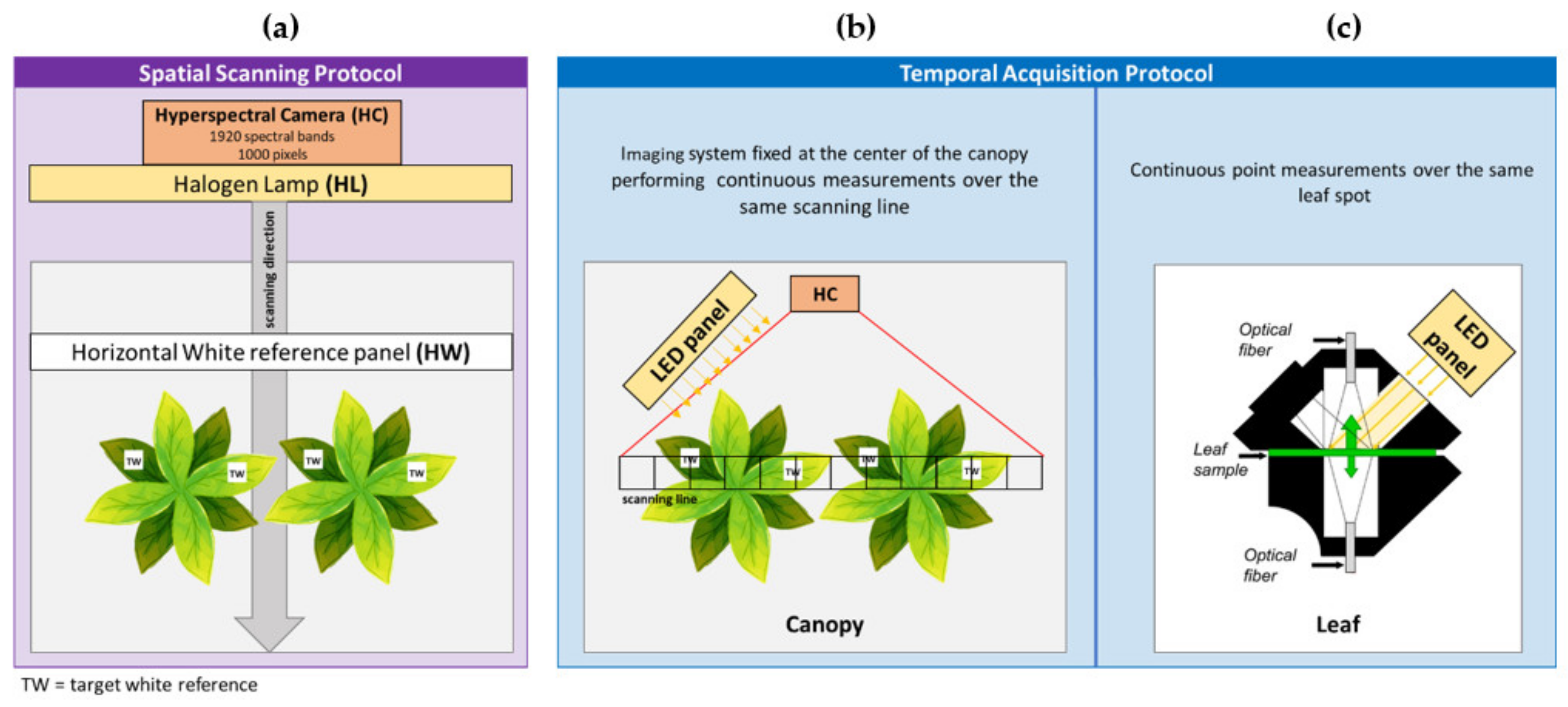
2.3.1. Spatial Scanning Protocol

The aim of the first protocol experiment was to measure the effect of the canopy structure on light propagation within the canopy, and its impact on the retrieved traits based on the measured reflectance spectrum. A large (5 × 40 cm2) rectangular horizontal white reference panel (HW, horizontal white reference) was placed at the distance of 40 cm from the imaging spectrometer in a fixed position perpendicular to the sensor optical plane and covering the entire sensor field of view (FOV) (Figure 1c and Figure 2a).
In order to expose the TOC leaves with the same illumination intensity as the HW panel, the pots were placed on a height-regulated tray and leveled to the same height.
The HW spectral measurement represents the TOC incoming radiance (LTOC-H), which implies the assumption of having the same illumination conditions over all plant leaf surfaces, regardless of their orientation or position within the canopy. To estimate the real incoming radiance arriving at each leaf-target surface (LLeaf-T), small 1 × 1 cm2 and 1.5 mm thin white ODM-98 (GigahertzOptik GmbH, Türkenfeld, Germany) reference panels (TW, target white reference) were attached with double-sided tape to several leaves with contrasting orientations, located at different depths of the canopy vertical profile, but always visible in the sensor nadir FOV.
The scanning protocol began with switching off the halogen lamp to measure the dark current of the scanning instrument (n = 5), followed by switching on the halogen lamp and measurement of the scanning area including the HW panel and the canopy with TW panels placed onto the leaves. This experimental set-up implies some particularities regarding the illumination and observation geometry. Due to the nadir-positioned halogen lamp and hyperspectral camera system arrangement, for all the scans, the camera FOV points to the plant surface exposed to direct illumination.

2.3.2. Canopy Temporal Acquisition Protocol

The second scanning protocol was developed for characterizing the dynamic variability in reflectance independently of the canopy structure and leaf orientation but instead focusing on the pigment dynamics upon photoprotection. For this protocol, we used the illumination panel composed of cool white LEDs providing a broadband 400–780 nm spectrum at a maximum intensity of 2000 μmol m−2 s−1 (Figure 2b). The panel with dimensions of 27 × 81 cm was placed on one side of the metallic frame under an angle of 45° pointing to the canopy. To measure the dynamic response in reflectance induced by the adaptation of the leaves to saturating light, we exposed the 2 h dark-adapted beech saplings to the saturating LED panel illumination for 25 min, recording the transition from dark-to-light. For this, the HySpec VNIR camera was fixed above the center of the canopy and the continuous recording of a single-pixel line happened at a rate of 45 fpm (Figure 2). This protocol was repeated for the beech saplings grown under the different illumination conditions (i.e., SU, SS and SH). We defined the beginning of the transient as t = 0 min and the end as t = 24.5 min and calculated the ∆ Reflectance for the course of the transient by subtracting the reflectance at t = 0 min for each measurement.

2.3.3. Leaf Temporal Acquisition Protocol

A similar experiment as the one described in the previous section was designed for capturing rapid reflectance and PRI changes at the leaf level. Here, we inserted a dark-adapted leaf inside the FluoWat leaf clip [37] with the leaf clip illumination opening towards the saturating light of the LED panel (Figure 1d and Figure 2b). The protocol was applied only for SU leaves, to verify the leaf spectral changes in parallel to the different xanthophyll pool changes. We followed a protocol described in [38], using a spectral integration time of 136 ms to record single spectra continuously for 20 min. At the end of the measurements, a white ODM-98 (GigahertzOptik GmbH, Türkenfeld, Germany) reference panel was inserted and measured inside the leaf clip. By using a short-pass filter, cutting off the incoming light beyond 650 nm, we could also observe changes in emitted Chl a fluorescence, indicative of changes in light-harvesting antenna during the so-called Kautsky effect [39].

2.4. Integrating Sphere Leaf Reflectance and Pigment Analyses

To obtain a reference value of leaf reflectance under standard illumination conditions for each sapling treatment (SU, SS and SU), the sampled leaves were measured also inside a Labsphere integration sphere RTC-060-SF (Labsphere Inc., North Sutton, New Hampshire, NH, USA) illuminated by a Koehler illuminator KI-120. Hemispherical reflectance and transmittance measurements were taken for leaves randomly sampled from the canopies by using the integrating sphere with a FieldSpec spectroradiometer (ASD Inc., Boulder, CO, USA) through an optical fiber [40]. The leaf reflectance measured in the integrating sphere is referred to as RLeaf-S. To show the spectral variability due to the biological variation within each treatment, we calculated the spectral standard deviation.
After measuring RLeaf-S the leaf samples were punched as leaf disks of 1 cm2 in diameter and immediately frozen at −80 °C. Chlorophyll a and b and total carotenoid pigment pools were chemically extracted with acetone solvent and analyzed by spectrophotometry using a UV-VIS absorption spectrophotometer (UV/VIS, Unicam, UK) according to the protocol described by [41]. Samples for the analysis of the dynamic xanthophyll pigments, i.e., violaxanthin (Vio), antheraxanthin (Ant) and zeaxanthin (Zea), were collected and analyzed from overnight dark-adapted plants and light-exposed leaves. For the sun-adapted leaves, samples were also collected at different time intervals of light exposure (in 4, 8, 12, 16 and 20 min), to investigate the conversion rate of the dynamic xanthophyll pool. Content of individual xanthophyll pigments was quantified with HPLC analyses of the samples, carried out using an Agilent 1200 HPLC-DAD system (Agilent, Santa Clara, CA, USA), equipped with a LiChroCART RP-18 (250 4 mm, 5 mm) chromatographic column (Merck, Germany), according to the protocol described in [42].

2.5. Spatial Scanning: Image Pre-Processing

Before extracting the desired information from the spatial scanning protocol, the images taken during this protocol experiment required a specific pre-processing. In particular, the images’ specular reflection and multiple scattering were characterized. The image processing, data quality assessment, and data analysis were performed using Python version 3.6 (Python Software Foundation, Beaverton, OR, USA) and ENVI version 5.0 (Exelis Visual Information Solutions, Boulder, CO, USA). Employed python modules were: Spectral Python v. 0.19, Numpy v. 1.14, Pandas v. 0.23 and Matplotlib v. 3.0 [43].
First, the camera electronic noise was corrected by subtracting the dark current (DC) image from each hyperspectral image. This process was done by calculating an average of five DC scanning lines acquired in total darkness and executing a line-by-line subtraction of the average DC spectrum from the entire image.
Second, to assess the impact of the specular reflection and multiple scattering in the images, the spectral angle mapper (SAM) function [44] was applied to classify the image in vegetation and non-vegetation pixels. The applied threshold value to distinguish vegetated and non-vegetated pixels was 0.41 radians. For the filtered vegetated pixels, we applied the Normalized Difference Vegetation Index (NDVI) [45] to quantify the specular reflection (Equation (1)). To reduce the impact of random noise in the index retrieval, reflectance values were obtained by averaging the neighboring spectral bands as follows:
N D V I =   R ¯ 800 803   R ¯ 670 673   R ¯ 800 803   +   R ¯ 670 673   ,
The inherent wavelength characteristics used to compute the NDVI made this index useful to detect leaf specular reflection effects. NDVI is to a large extent insensitive to changes in light intensity, i.e., similar spectral signatures but with different overall spectral intensities produce similar NDVI values. However, because the leaf spectrum has a low red reflectance with respect to the near infrared (NIR), opposed to the white light source, it results in a good proxy to sense the specular reflection within the image. Based on this approach, an NDVI threshold range was established to separate the leaf surface affected (NDVI 0.66–0.82), and unaffected by specular reflection (NDVI 0.82–1). Figure 3 presents the result of applying the NDVI threshold, with the yellow color indicating the image pixels affected by the specular reflection that were filtered out for further analysis.

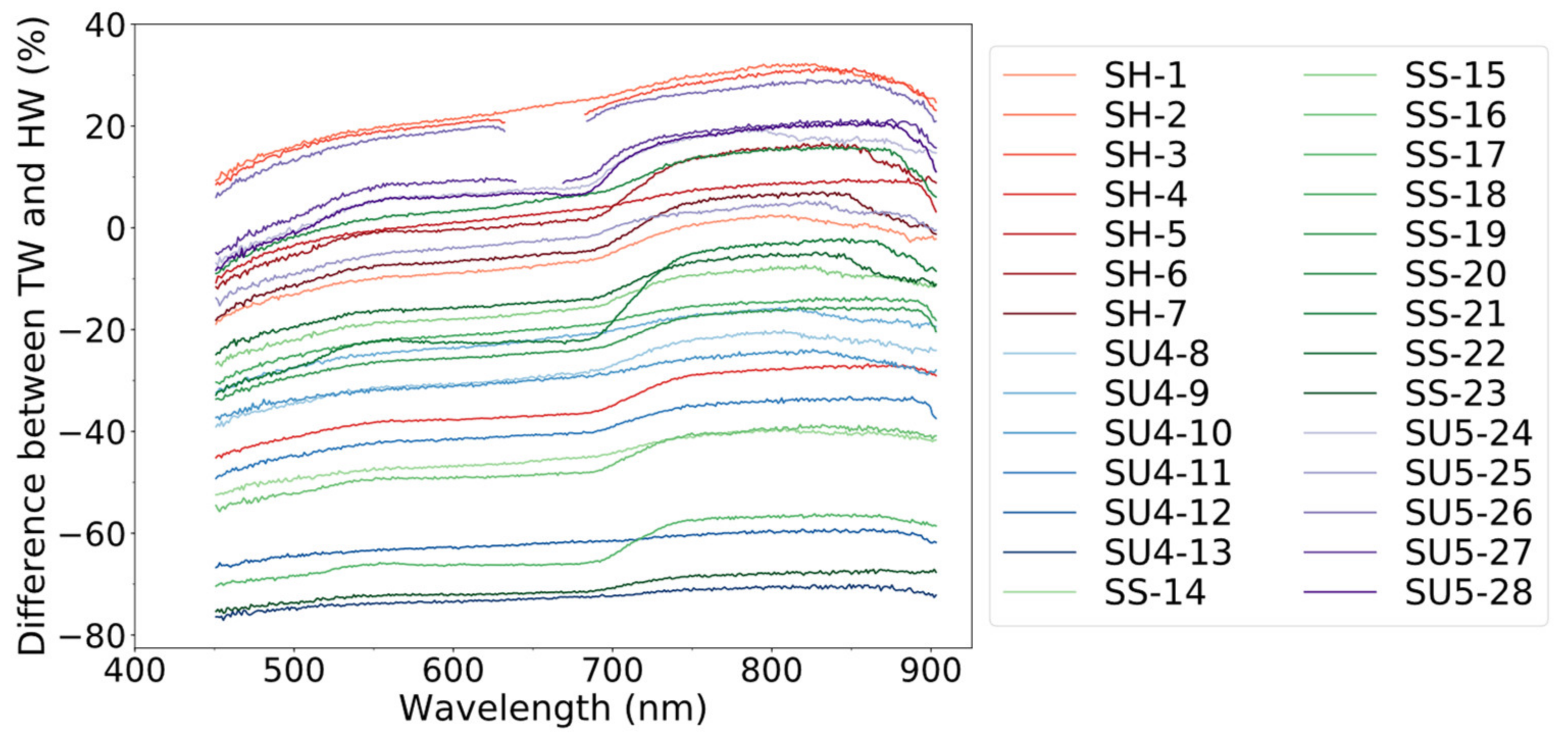
2.6. At-Target and Horizontal White Reference Comparison

The white reference panels placed on top of selected leaves (TW) aim to quantify the actual at-target illumination conditions (Figure 4).
By comparing the incoming radiance measured using the TW and HW we were able to evaluate the spectral differences between both protocols. To quantify the offset in illumination conditions, due to the different orientations/positions of the leaves inside the canopy, the difference between both reference panels was computed based on the average value of their respective areas as shown in Equation (2):
D i f f e r e n c e   r e s p e c t   t o   t h e   H W = D N T W D N H W D N H W   ,
where DN are digital numbers of the light reflected by the measured reference panels.

2.7. Top of Canopy and At-Target Leaf Reflectance and Their Derived Vegetation Indices

To obtain the at-target-leaf reflectance (RLeaf-T) in the range of 400–800 nm, ENVI’s region of interest (ROI) toolbox was used to select a representative number of pixels for each leaf of the same orientation as the attached TW. Then, dividing the averaged spectrum of the leaf ROI (with an average of 35 pixels per ROI) by the TW ROI (with an average of 50 pixels per ROI), the RLeaf-T was calculated for 5–10 leaves per image (Figure 4).
The TOC reflectance for the complete image (RTOC-H) was computed, omitting the regions with specular reflectance, dividing the entire image line-by-line by the HW average spectrum. In order to compare the leaf target reflectance with the TOC reflectance spectra, the same leaves’ ROIs used to compute RLeaf-T were applied to the RTOC-H images, extracting the ROI’s pixel-averaged reflectance spectrum of each leaf (RLeaf-H) from the image. Finally, for individual leaves of each beech canopy, the reference reflectance was obtained with the integrating sphere measurements (RLeaf-S), as described in Section 2.3.
In summary, four different reflectance spectra, listed in Table 1, were evaluated in this study to analyze (1) the structural and biological effect, and (2) the spectral variability in their reflectance shapes.
Besides the aim of highlighting the variability of the entire reflectance spectrum due to biophysical and architectural effects on at-target incident light, two vegetation indices (VI) were additionally computed using RLeaf-H and RLeaf-T.
The first VI is the Meris terrestrial chlorophyll index (MTCI), calculated from Equation (4), which shows the sensitivity to the actual canopy chlorophyll content [46]:
M T C I = R ¯ 752 754 R ¯ 707 709 R ¯ 707 709 + R ¯ 680 682 ,
The second VI is the photochemical reflectance index (PRI), according to Equation (5), which was traditionally used as a proxy of the dynamic xanthophyll transformation induced by an excessive light exposure [10,11]:
P R I = R ¯ 529 531 R ¯ 568 571 R ¯ 529 531 + R ¯ 568 571 ,
To reduce the instrumental noise effects in the index computations, the average reflectance values used for MTCI and PRI calculation were obtained by averaging the neighboring bands.

2.8. Statistical Analysis and Intercomparison Methods

Depending on the type of data, two different approaches were applied to evaluate the results of this study. The Fligner’s test was computed to discern between different types of data variance. Subsequently, data with the same variance were compared using the common Student’s test. The Welch’s t-test was used when analysis of variance assumptions (i.e., normal distribution and homogenous variance of data) were violated. All these calculations were made with Python’s library Scipy version 1.1. The analyses were applied to assess the statistical equality of data pairs in each image with and without specular reflection, and of data pairs referred to vegetation index values obtained per light growing treatment.
With the aim of spectrally quantifying the difference between the white reference (HW and TW) used to compute reflectance, the absolute reflectance difference between RLeaf-H and RLeaf-T was calculated:
A b s o l u t e   r e f l e c t a n c e   d i f f e r e n c e = R L e a f - H R L e a f - T   ,
where RLeaf-H and RLeaf-T are the reflectance spectrum obtained with the horizontal and target panel respectively.
Spectral variability due to structural, biological, and photochemical effects were studied based on the variability (either by standard deviation or reflectance differences measured) within each dataset, for each treatment.
The PRI trend values obtained during the TOC light transient were compared among treatment. During the transient phase, the reflectance spectral shape changes over time. In order to evaluate not only the differences in the (dark-adapted) PRI value but also the photoprotection dynamics, we applied a t-test for the first PRI value upon sudden illumination, and for the ∆PRI value for each treatment. The ∆PRI was calculated with the first (t = 0 min) and last (t = 24.5 min) measurement of each transient (Equation (6)).
Δ P R I = P R I t = 0 P R I t = 24.5 ,
where P R I t = 0 and P R I t = 24.5 are the PRI values obtained respectively at the beginning and end of the transient.

3. Results

We first present results on leaf and canopy reflectance variability in the PRI region caused by an incorrect characterization of the at-target radiance (Section 3.1, Section 3.2 and Section 3.3). Approximately 85% of samples presented a negative difference value, indicating that the light arriving at HW is higher than the light reaching TW. Second, the PRI dynamics triggered by quick xanthophyll pool variations and/or Chl vs. Car long-term changes are evaluated (Section 3.4 and Section 3.5). When comparing vegetation index values computed from RLeaf-H and RLeaf-T, we observed a mean overestimation of 2% for MTCI-HW for all treatments. For PRI an average underestimation of 31% was detected for PRI-HW. Finally, we compare the shape and magnitude of spectrum variations due to the studied factors (Section 3.6). The largest spectral variability is due to the structural affection, followed by the biological and quick photochemical effects. Giving the instrumental noise the smallest variability in the reflectance spectrum.

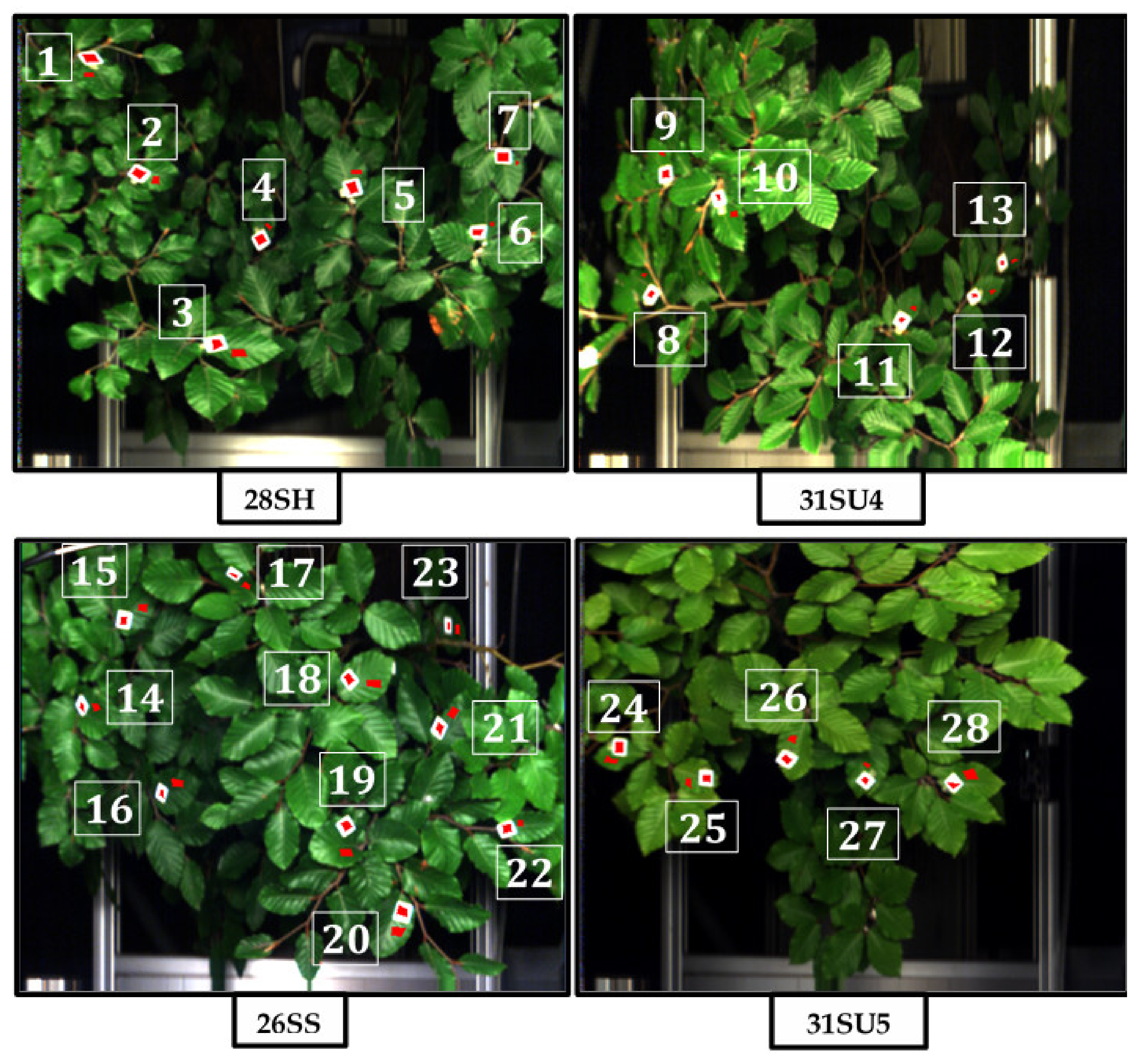
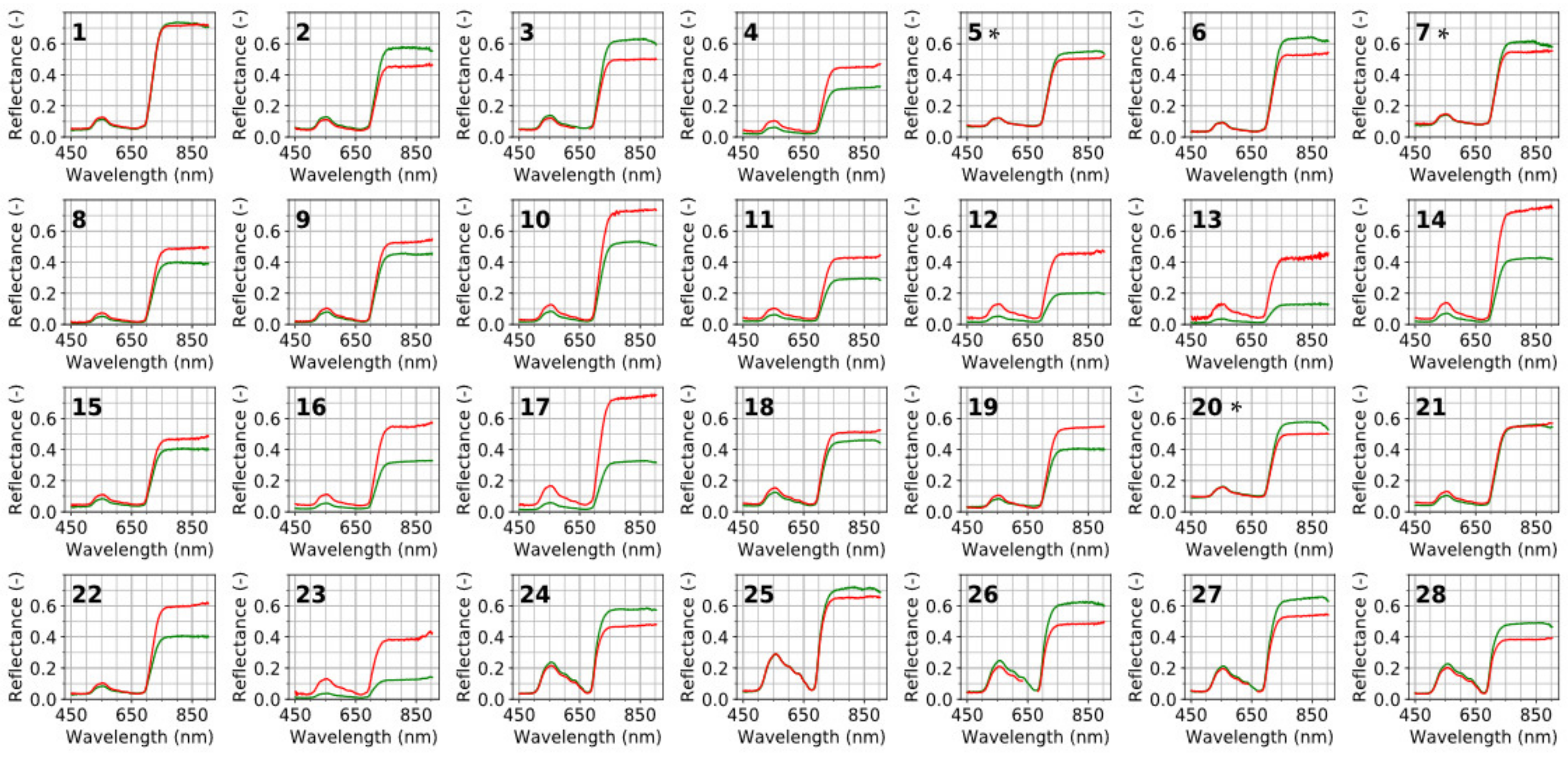
3.1. Difference in Leaf Reflectance for Target vs. Horizontally Placed White References (RLeaf-T, RLeaf-H)

The specially proposed set-up allowed us to evaluate the reflectance differences due to illumination conditions reaching the target and horizontal white reference panels (Figure 5).
Our results revealed that for all treatments and leaves shown in Figure 4 the difference between TW and HW measured reflected radiance consistently increased with increasing wavelength. The difference showed a slight peak at the PRI region and a notable rise at the red-edge region of the spectrum (~700 nm), with maximum values between 800–900 nm. Approximately 85% of samples presented a negative difference value, indicating that the light arriving at HW is higher than the light reaching TW. There was no evidence of grouping the results by treatment. The difference was dependent only on the relative location of TWs.
When analyzing the leaves, reflectance computed with the TW and HW (Figure 6) a consistent pattern was found for all treatments and leaves. In the PRI spectral region, 64% of sampled leaves presented similar reflectance patterns. In contrast, for the red edge and near-infrared region of the spectrum, 57% of samples presented higher values when TW was used. For the remaining 43%, reflectance computed with HW showed higher values. Interestingly, samples 1 and 21 present similar values along the entire spectrum, demonstrating differences between TW and HW close to zero. On the other hand, samples 12, 13, 17 and 23, having a value of −60% and −80%, present the highest discrepancies between TW and HW computed reflectance spectrum. Consequently, a mistake introduced by a wrong incoming irradiance measurement affects the full VNIR spectral range of a vegetation surface reflectance.

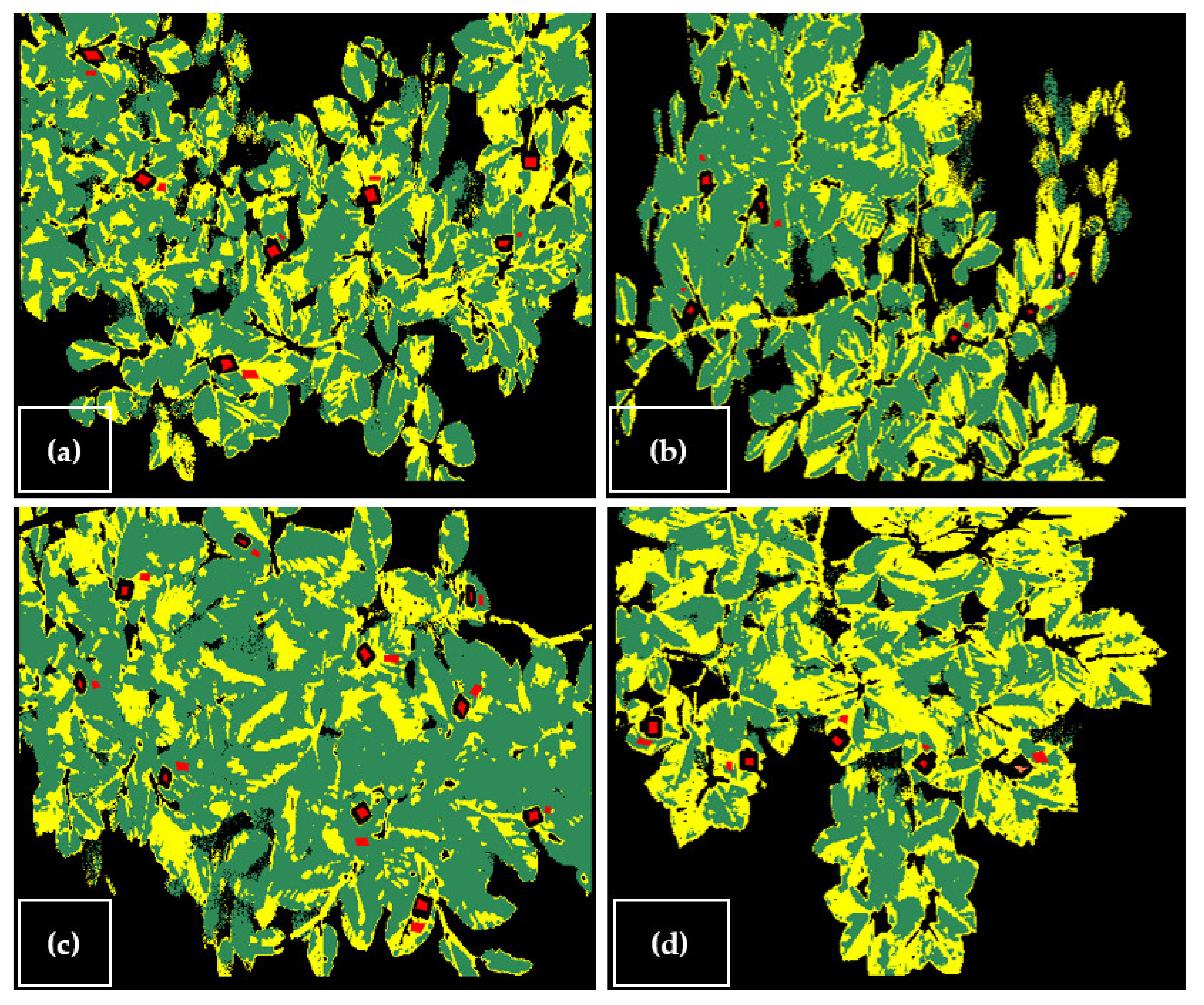
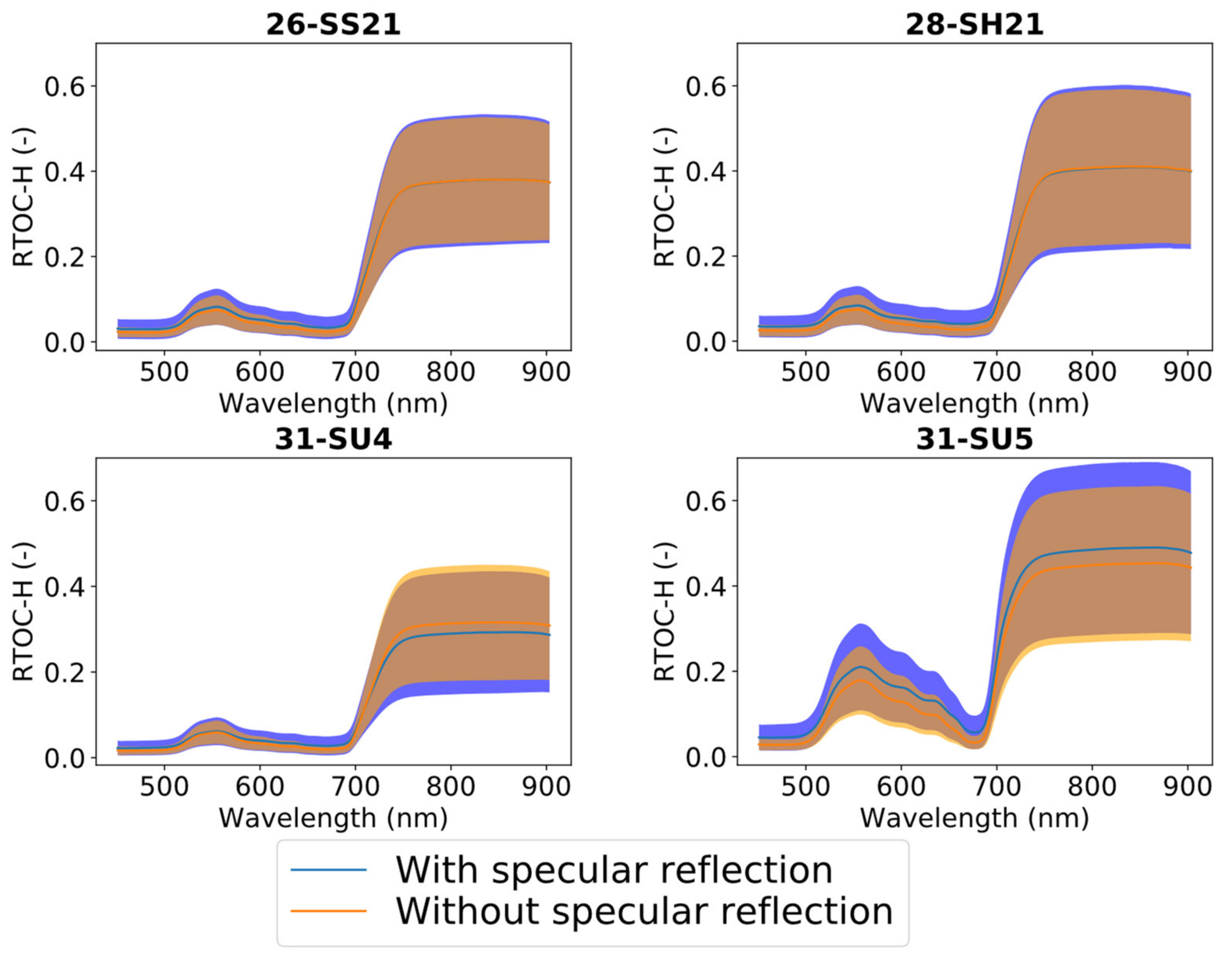
3.2. Impact of Specular Reflection on Canopy Reflectance (RTOC-H)

When plotting an image average TOC reflectance computed using HW (RTOC-H) with and without a specular reflection (Figure 7), SU replicates presented a higher absorption in the PRI region, as well as a higher reflection in the rest of the visible and near-infrared part of the spectrum than SS-SH plants.
For all study cases, specular reflection slightly increased the overall reflectance value at the PRI region and red-edge part of the spectrum. However, two different patterns were observed in the near-infrared region. On the one hand, similar mean values were observed between corrected and not corrected images for SS and SH. On the other hand, the corrected image present higher mean values than the non-corrected for SU4, while an opposite pattern was found for SU5. Overall, statistical differences between the dataset with and without specular reflection were found with 95% of confidence. Henceforth, from now until the end of the manuscript, all results will refer to the reflectance corrected for the specular reflection.

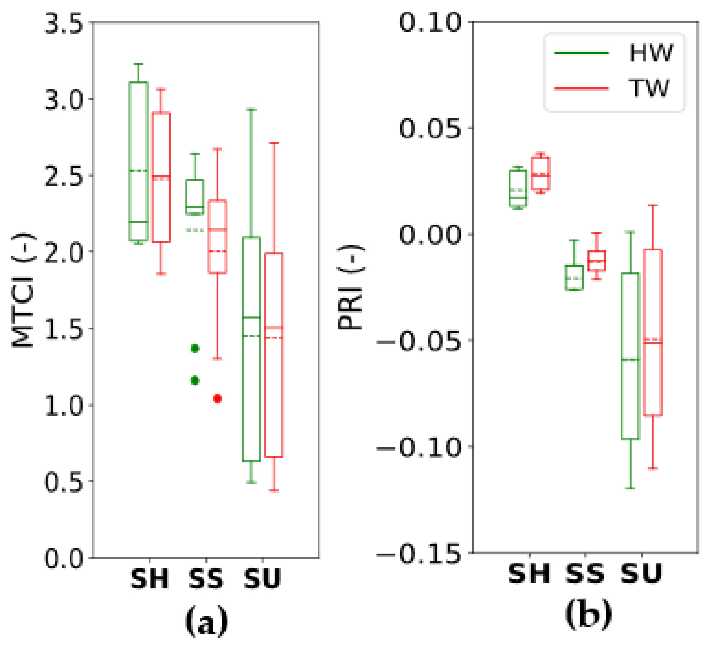
3.3. Vegetation Indices Computed from Leaf Reflectance (RLeaf-T, RLeaf-H)

Using the reflectance spectrum without the specular reflection, MTCI and PRI indices were calculated. When comparing MTCI values computed from RLeaf-H and RLeaf-T, we observed a mean overestimation of 2% for MTCI-HW when compared to MTCI-TW for all treatments (Figure 8).
In contrast, an average underestimation of 31% was detected for PRI-HW over PRI-TW. Similar results were found for MTCI and PRI indices retrieved from RTOC-H (data not shown).
MTCI values revealed a higher chlorophyll concentration for SH and SS plants compared to SU. MTCI values showed significant differences in chlorophyll concentration between SU and both SS and SH light treatments, with a confidence probability of 95%. However, the difference between SS and SH light growth conditions was statistically insignificant.
The PRI index indicated the highest photoprotection for SU and the lowest for SH plants. The SS samples had intermediate PRI values, fitting in-between the above-mentioned. Differences in PRI for all three light growth treatments were statistically significant with a confidence level of 95%. Additionally, SH had positive index values, whereas SS and SU demonstrated exclusively negative PRI values.

3.4. Pigment Pools for Different Treatments and Effect on PRI Measured in Integrating Sphere

Consistent differences between the studied growth light exposure treatments SH/SS and SU were observed also in pigment composition. The SU leaves contained a lower pigment concentration per surface area, especially a lower Chl a and Chl b content (Figure 9a).
Due to its lower Chl content, SU leaf reflectance spectrum measured in the integration sphere showed lower absorption in the blue and red regions, but higher reflectance in the green region (where the PRI bands are located, Figure 9b—top). SU samples were clearly differentiated from the other two treatments. Figure 9b—bottom shows the difference considering the pigment pool and photoprotection level. Consistently, SU leaves showed a larger relative xanthophyll pool to Chl a pool (Figure 9c). When SU leaves were exposed to a saturating light, the impulse converted most of the violaxanthin to zeaxanthin within 4 min.

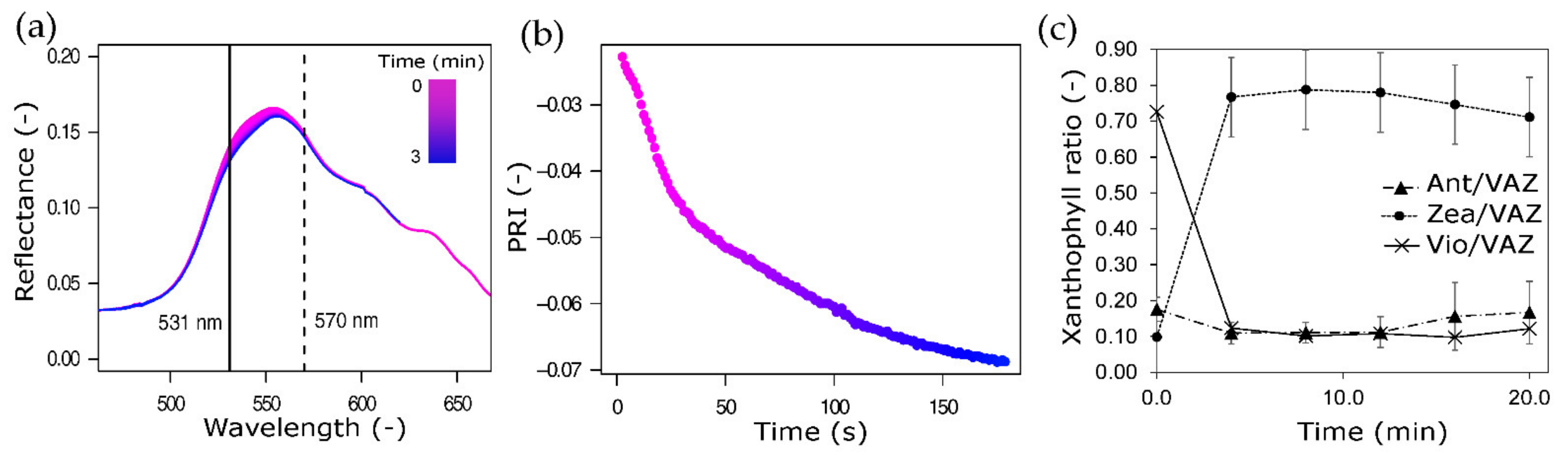
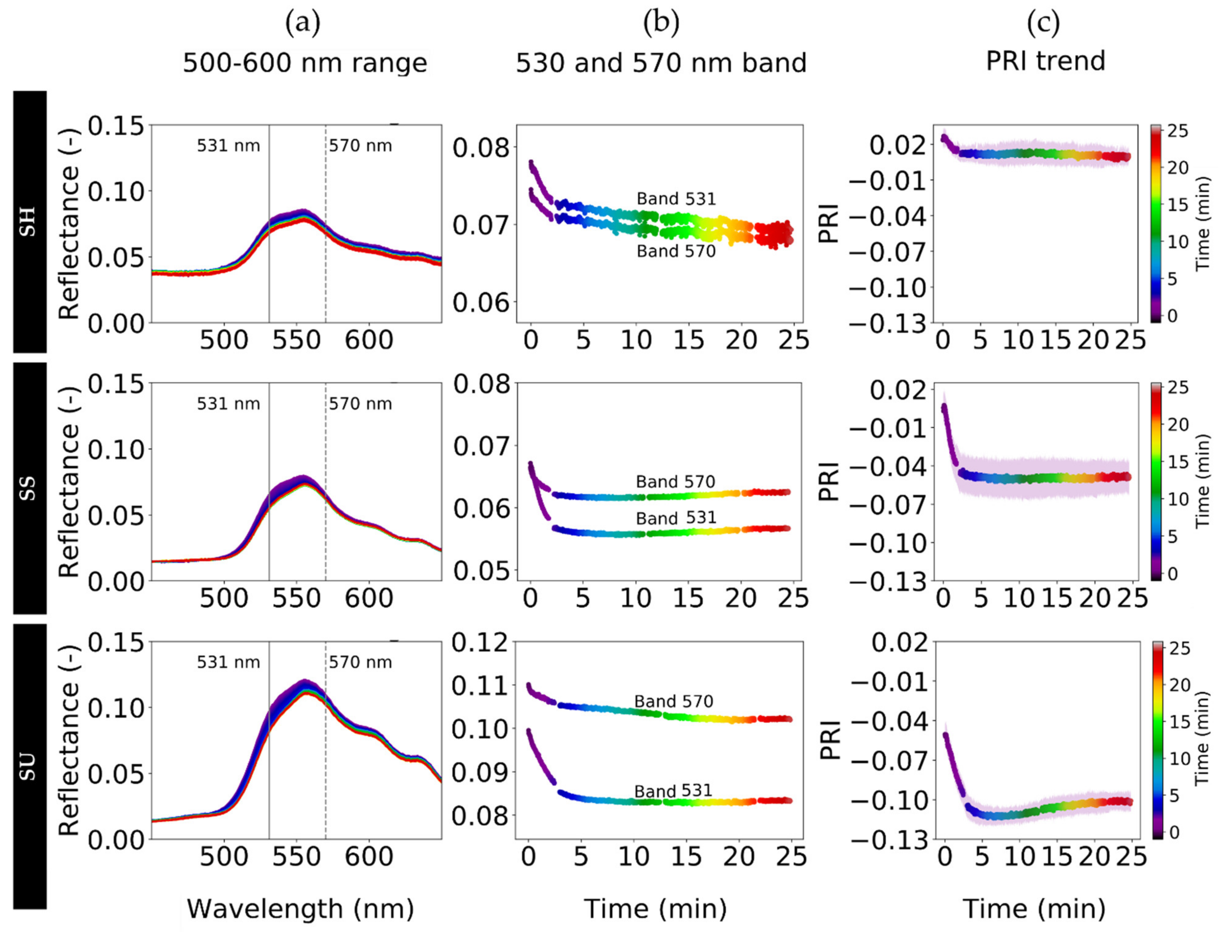
3.5. Quick Dynamic Reflectance Changes and Their Effect on PRI

At leaf level, quick photochemical reflectance changes in the PRI region appear within the first minutes after light exposure (Figure 10).
During this fast adaptation to excessive light, PRI shows a quick decrease together with the xanthophyll pool transformation of violaxanthin to zeaxanthin (Figure 10b,c).
The reflectance change pattern showed consistent with our observations at the canopy level. Figure 11 shows the temporal trends of the reflected signal for a light-exposed pixel in the line scan of respectively the SU, SS and SH canopy, recorded as illustrated by the protocol in Figure 2b.
The temporal reflectance dynamics of the plant canopy surface were recorded as time series of the reflected signal during 20 min after a sudden light exposition of dark-adapted canopies (Figure 11a) and from the PRI bands (Figure 11b) the index was subsequently calculated (Figure 11c).
To compare transients between the treatments, we selected pixels from the line scans that were exposed to comparable light intensities. This was done based on comparable reflectance values within the line recordings. All cases show a decreasing trend in the 500–600 nm range of a reflected signal until an equilibrium state is reached. In the red and far-red regions, the signal showed the effect of the decreasing fluorescence as well (results not shown). The largest decrease of the reflected signal change occurred within the first minutes of the protocol, indicated by purple color.
All three cases show a similar signal decrease in the 500–600 nm region, but with slightly different behavior in PRI bands. For the SS case, one can see first a large decrease of the PRI bands, followed by a slow increase over the experiment time. The band at 531 nm has a more remarkable decrease within the first phase. The same occurred for the SU canopy, where the differences are even larger. The 570 nm band decreased notably over the first two-thirds of the time and only slightly after a stabilization, while the 531 nm band decreased only during the first three minutes. As a result, the PRI trends calculated from these bands reveal slightly different dynamics per treatment. First, it can be noticed that the starting PRI value at t = 0 for the dark-adapted starting point is higher, following the order SU > SH > SS. This difference between all the treatments was statistically significant at 95% interval confidence. Further, the difference in PRI during the transition (i.e., ΔPRI) also increases in this order, with the SU case showing the largest difference over time. In contrast with the ΔPRI from SU and SS which show no statistical differences between them, the SH case showed statistical differences between the other both at 95% interval confidence. The SU case also shows, besides the lowest PRI values, a gradual slow increase of the PRI values in the second half of the transient. This can be attributed to a further decrease of reflectance at the 570 nm band.

3.6. Spectral Variability of Structural, Pigment and Photochemical Effects

In the last step we verified the spectral behavior of the structural and biological, both intrinsic and dynamic, effects on the reflectance signal for the different treatments. The results of the different spectral variability sources in the signal are compared in Figure 12.
The associated spectral variability has a different magnitude depending on the effect. The structural effect as illustrated in Figure 6 and Figure 7 strongly affects the reflectance variability, up to a difference of 5% in the 500–600 nm region for the SU and SS treatments. The SH canopy differences in reflectance remained below 2% for the 500–600 nm region.
At the leaf level itself, the effect of intrinsic pigment contents showed a clear effect on the reflectance (Figure 9b), resulting in a reflectance variability illustrated in Figure 12b. The maximal variability in reflectance is shown for the sun-adapted leaves, showing a standard deviation of 0.035 at 570 nm. The sun-shade and shade-adapted leaves show standard deviation values around 0.01 or 1% reflectance in this region.
The third source of variability ordered by magnitude is shown by the variability due to the dynamic photochemical responses. In Figure 12c, the reflectance change is presented showing the variability recorded during the transient experiment at canopy level. The magnitude of this variation is small, around 1–1.5% of the reflectance, and similar for all the treatments, with a higher standard deviation for the SU treatment. The subtle remarkable difference concerning the previous shape variabilities, due to the structure and intrinsic pigment contents, can be seen from the position of the peak of these spectral difference shapes.
The last source of variability for this experiment was instrumental behavior. The instrumental noise of the radiometric measurements from the TOC measurements was evaluated obtaining an error in the spectral range of 500–600 nm of less than 0.02% in reflectance (data not shown).

4. Discussion

When a remote sensing study aims to monitor the vegetation dynamics, it must consider external factors that can create a bias between the actual plant status and the estimated physiological parameters retrieved through spectroscopy methods. This is challenging in natural environments, where the complexity of characterizing all confounding factors (i.e., light reabsorptions, multiple scattering by surrounding objects, and fast variation in light intensity among others) is not trivial. These complexities impose necessities for a trade-off between the need of characterizing each driving variable and the capability to measure them with a required accuracy using standardized protocols. The objective of this study is to investigate the variability of the PRI spectral region caused by: (1) protocol-related incorrect incoming radiance characterizations, (2) intrinsic Chl and Car pools induced by long-term (seasonal) adaptations, and (3) quick xanthophyll pool dynamics induced by short-term light adaptations.
Traditionally, for both indoor and outdoor experiments, the incoming radiance reaching the monitored plant is characterized using a large-size white horizontal panel placed near the studied target [47,48]. However, the results of this study show that the placement of the white reference impacts quantification of the at-target incoming radiation and consequently the computed vegetation reflectance spectrum and derived spectral indices. Depending on the leaf orientation and leaf location inside the canopy, different spectral signatures were found when comparing TW- and HW-measured incoming radiance. On the one hand, a similar spectral signature was found between the TW and HW protocols for fully illuminated leaves, resulting in wavelength-independent differences. On the other hand, for leaves located deeper inside the canopy and/or with a high inclination angle, different spectral signatures were observed between TW- and HW-based reflectance (Figure 5). Two main processes could explain that within the PRI region difference in reflectance between the TW and HW protocols was around 5%, while the near-infrared region showed differences up to 10–20% (Figure 5 and Figure 12a). First, top-canopy leaves absorb most of the incident visible light, in contrast to the NIR photons that are highly scattered and penetrate [49]. Second, according to the inverse-square law, the light intensity decreases with the distance from the illumination source. This effect is corroborated by a direct relationship between the TW vs. HW values and the at-target white panel TWs fully exposed to light (e.g., SH-2 and SH-3, Figure 5). These had a positive difference value, meaning that a higher amount of light reached TWs compared to HWs targets. In contrast, incoming radiance measured from TW samples located deeper inside the canopy (e.g., SH-4), showed high negative difference values, reaching nearly −80%.
At 531 nm, 57% of the samples presented higher reflectance values when the vegetation spectrum was computed using the TW with respect to the HW protocol. This resulted in an underestimation of the reflectance factor derived by the HW panel protocol. The consistency found for all replicates and treatments points out that the main driver of reflectance differences is not the difference in leaf pigment composition (induced by the imposed illumination growing conditions) but rather a change in the reference illumination throughout the canopy. The minor spectral variability, observed in the samples of the SU-5 canopy (Figure 6, samples 24–28), was caused by the arrangement of the studied leaves, since all of them had a similar position and orientation in the canopy, resulting in a high exposure to direct illumination. In concordance with other studies [26,50,51], the deviation in the computed reflectance spectrum using incorrect values of incoming radiance introduced an error in derived vegetation indices. Consequently, depending on used spectral wavelengths, it is possible to underestimate or overestimate the index-assessed plant physiological status. In the case of PRI interpretation, for instance, a general overestimation of the photoprotection status (underestimation of PRI values) was observed (Figure 8b, samples 24–28), caused by the arrangement of the studied leaves, since all of them had a similar position and orientation in the canopy, resulting in a high exposure to direct illumination. In contrast, the leaf chlorophyll content estimated with the MTCI index was generally overestimated (Figure 8a). These results are in concordance with studies based on RTM where wrong assumptions on actual target irradiance reach up to 32% for the PRI obtained in [49]. PRI is slightly underestimated by up to 5% in [52].
Plants rely on flexible physiological and structural patterns of growth that allow them to adapt to different environmental conditions, including temperature, nutrients-water availability, and irradiance [53]. In this study, different light-growth treatments were inferred to simulate the various light growing conditions, to which plants are exposed in natural environments at the seasonal scale. This translated into different adaptative responses occurring on a diurnal and seasonal cycle. The set of protocols showed the distinctive effects of both Chl versus Car ratio (constitutive responses), as well as the xanthophyll pool (facultative responses) on the reflectance and PRI for SU, SH, and SS adapted leaves. These results are consistent with [11,24]. SH and SS leaves presented a higher chlorophyll versus carotenoid ratio and a lower relative xanthophyll versus Chl a pool, when compared to SU leaves (Figure 9b,c) indicating a stronger photoprotection capacity of the SU leaves. The observed chlorophyll versus carotenoid differences and xanthophyll pool among treatments are due to the plant’s adaptation to the light environment. From winter to summer, the prevailing illumination conditions are changing and plants are adapting the size of their photosynthetic light-harvesting complexes accordingly [54]. Furthermore, top-canopy leaves will also develop a higher photoprotection than shaded bottom-canopy leaves [25]. These long-term adaptations, in combination with slow and fast pigment adaptations (Figure 9), translate into a different Car/Chl and xanthophyll pigment pools, and consequently in a different canopy reflectance spectrum [55]. Larger Car/Chl of the SU-adapted leaves translates into a higher reflectance within the 500–600 nm spectral range (Figure 12), when comparing specific treatments, resulting in lower PRI values for SU compared to SH and SS samples. While the reflectance variability due to intrinsic Chl versus Car pools is strongly pronounced for the SU leaves (Figure 12b), reflectance variability due to xanthophyll behavior is more similar between the treatments (Figure 11 and Figure 12c). During the light transients for all three treatments, the PRI changes appeared nearly simultaneously with the VAZ pool changes indicating a conversion of violaxanthin to antheraxanthin and zeaxanthin (Figure 10c). Nonetheless, a statistically probed larger ΔPRI observed for SU-adapted leaves further indicated a larger xanthophyll pigment pool size (Figure 9c and Figure 11). As pointed by Gamon and Berry [25], when comparing the light transient curves, the PRI offset at the dark-state indicates different constitutive pigment pool sizes between treatments, whereas the PRI kinetics illustrate the facultative effects of the xanthophyll pool conversion. Because the facultative and constitutive effects on PRI are strongly interrelated, it is challenging to differentiate between the short-term xanthophyll conversion and the long-term pool’s size effects based on only a two-band index such as PRI. In this regard, the quantification of the leaf pigments’ pools and their specific spectral behavior in time and space is crucial before using PRI as a proxy of NPQ [20]. At the leaf level, we found similar spectral behavior in the PRI region, while the observations at canopy level showed some minor shape variability (Figure 10 and Figure 12c). Within the canopy, variability found may be higher than 1% in the PRI region due to the additional confounding effects of the structure (Figure 5). Despite these large variability and deviation effects to overcome, the optical changes in the PRI region due to xanthophyll-related energy distribution (Figure 10a) have been designated to specific spectral underlying behavior [20]. As showed in Section 3.5, the exposure of a dark-adapted plant to intense light, produces quick changes in the measured reflectance spectrum shortly after a sudden strong light exposure. Regarding the time frame, main spectral changes occurred during the first 3 min, independent of the leaf or canopy spatial scales [11,20]. Therefore, unintentional high-intensity illumination could lead to erroneous conclusions regarding the plant physiological status.
To properly propagate the dynamic physiological regulation processes taking place at leaf level towards remotely sensed canopy level measurements, one has to include in the protocol sampling strategies the characterization of the vegetation spatial and temporal heterogeneity. Here, we would like to highlight that in order to quantify a dynamic parameter as photoprotection, it is important to measure under light conditions similar to the plant light growing conditions and use a stable light source.
The benefit of leaf level measurements is not only an accurate characterization of the at-target incoming radiance but also characterization of full leaf optical properties, i.e., the reflectance-transmittance-and-absorption temporal dynamics. For non-destructive optical measurements of top canopy leaves, where the direct light is the main component of their illumination, we recommend the use of a leaf clip system coupled with a spectroradiometer (Figure 1d). The design of the FluoWat leaf clip, used in this study, allows for measuring each leaf under the same illumination and observation angles, which makes the measurements fully comparable. The main shortcoming of such leaf-level measurements is the time constraint. Since a single measurement might take up too few minutes, it limits the number of leaves that can be measured within a given period (e.g., ~1 h of stable environmental conditions would result in no more than 20–30 sample measurements when considering the time needed for displacement and leaf clip operations).
In case of top-of-canopy measurements, both point-based and image-based spectral optical systems could be used to monitor the vegetation. Point-based systems provide an integrated value for a specific field of view. These instruments have been widely applied for continuous temporal measurements over a limited area. In order to characterize the surface spatial variability is necessary to mount the point sensor in a mobile platform [56,57]. In contrast, image-based systems provide an opportunity to differentiate spatially components covered by the camera or imaging scanner field of view. This strategy allows to disentangle spectral artefacts introduced by non-photosynthetic surfaces (i.e., bare soil, branches covered by bark, etc.) and illumination effects (i.e., sunlit vs. shadow leaves, specular reflection, etc.) impacting the overall canopy signal. Moreover, by mounting an image-based sensor on a mobile platform, it is possible to map a larger area of interest or to create canopy 3D digital surface models using a photogrammetry approach applied on overlaying parts of images captured from two different viewing directions [58,59]. The main limitation of canopy-level measurements is the proper characterization of the incoming reference radiance and a light distribution inside the canopy. The use of small white reference panels attached to the leaves is, obviously, unfeasible for continuous measurements over large study areas. However, thanks to technical advances in the radiometry instrumentation, use of small radiometers (e.g., SpectraPen mini from the Photon Systems Instruments, Drásov, Czech Republic) distributed within the canopy might facilitate quantification of the incoming light at different canopy surfaces. A proper characterization of the radiation distribution within the canopy is crucial for an accurate estimation of the plant physiological status when using optical remote sensing techniques. In this regard, the use of computer-based radiative transfer models, that consider the interaction between the canopy and the direct, diffuse, and scattered light, is an efficient alternative to characterize and simulate the overall vegetation canopy complexity. Parameterizing the canopy leaf angle distribution (LAD) function, leaf area index (LAI), leaf clumping, fractional vegetation cover (FVC) and other structural features of these models is, however, necessary to simulate propagation of the light interactions from leaf to canopy measurements and to model a canopy photon escape probability. Two main radiative transfer approaches are used to model these interactions: (1) a “big leaf” approach (i.e., SCOPE model, [60]), which represents the vegetation surface as a unique horizontal layer (or vertical succession of layers) characterized by established turbid medium optical properties, and (2) a more detailed “3D heterogeneous architecture” of the studied vegetation (i.e., DART model, [61]), bringing the opportunity to distinguish different light interactions and leaf light adaptations inside the modelled canopy [62,63]. It is important to note that computational cost of the 3D canopy radiative transfer modelling could be challenging, especially for large study areas.
Finally, this study highlights the importance of setting appropriate observation and illumination conditions at canopy level when conducting an experiment to resolve pigment-related absorption properties, both intrinsically and dynamically. A wrong experiment design can increase the impact of specular reflection, mainly at the canopy level. The results of this study show the importance of confounding factors impacting the average reflectance factor starting from: (1) specular reflection, (2) reference of incoming illumination, (3) intrinsic leaf pigment pools, and (4) dynamic xanthophyll pools. The dynamic PRI optical changes measured at leaf level were observed in a consistent order also at the top of the canopy, which represents the xanthophyll conversion of the top-canopy leaves. Further work should focus on enhancing spectral decomposition techniques to disentangle specific drivers of canopy PRI.

5. Conclusions

Various vegetation canopy variables are affecting the light reaching a target surface. Our results corroborate the hypothesis that the horizontal white reference panel, commonly used to estimate the at-target surface incoming radiance, produces a bias between the real photosynthetic plant surface reflectance factor and the remotely estimated top-of-canopy reflectance factor. This discrepancy originates from differences in illumination spectral characteristics, as well as the intensity between the light arriving at a horizontal panel and the actual light reaching the leaves’ surfaces. The discrepancies captured in this work due to an incorrect irradiance estimation show this source of deviation as the highest bias compared with the biological, photochemical and instrumental variability. The differences in absolute terms between RLeaf-H and RLeaf-T reach up to 6% in 500–600 nm reflectance values. Photon multiple scattering from adjacent leaves, branches, and soil under the canopy causes a different wavelength-dependent spectral behavior. Due to the foliar pigments’ absorption, the radiation of wavelengths shorter than the red edge is absorbed more than the one of longer wavelengths, and these absorptions are dynamic, changing faster or slower depending on the local plant pigment pool adaptations.
Plants are adapting their pigment pools to maximize photosynthetic efficiency under changing environmental conditions and dissipate excessive energy. They have actively developed intrinsic long-term changes of the Chl and Car pools and quick xanthophyll pool dynamics as the photoprotection mechanism. The spectral variability in the PRI range due to the pigment pool is higher on leaves from SU and SS, showing reflectance standard deviation rounding the 3%. The analysis comparing the ΔPRI revealed statistical differences between the plants adapted to shadowed growing conditions and the other two growing conditions exposed to sun. Vegetation indexes, widely used to determine the vegetation’s physiological status, can be heavily affected by a wrongly measured incoming light characterization. In this study, we employed different protocols to improve the accuracy of remote sensing methods for characterizing the vegetation status. These improvements let to compare leaf and canopy scale measurements, disentangling between the spectral distortions of the spectrum. This approach evidences the vegetation PRI spectral dynamics, both at leaf and at canopy level, and facilitates the understanding of the structural and biophysical variability inside the canopy. Further characterization of these specific spectral behaviors through improved bottom-up approaches may help to understand and disentangle light-driven changes from the canopy reflectance impacts. Current (field) and future-planned (airborne) operational sensors aim to characterize the vegetation reflectance shape at high spectral and spatial resolutions, giving new opportunities to unravel the spectral dynamics given by structural, biological and photochemical drivers.

Author Contributions

Conceptualization, S.V.W., M.P.C.-M., L.A. and Z.M.; Data curation, A.M.-E.; Formal analysis, A.M.-E., S.V.W., M.P.C.-M., L.A. and J.M.; Funding acquisition, J.M.; Investigation, A.M.-E., S.V.W., L.A. and Z.M.; Methodology, S.V.W., L.A. and Z.M.; Project administration, J.M.; Resources, Z.M.; Software, A.M.-E. and L.A.; Supervision, S.V.W., M.P.C.-M., L.A., Z.M. and J.M.; Writing—original draft, A.M.-E., S.V.W. and M.P.C.-M.; Writing—review & editing, S.V.W., M.P.C.-M., L.A., Z.M. and J.M. All authors have read and agreed to the published version of the manuscript.

Funding

AM-E is currently funded by AVANFLEX project (Advanced Products for the FLEX mission), n° ESP2016-79503-C2-1-P, Ministry of Economy and Competitiveness, Spain”. SVW is funded by the “Algorithm retrieval and product development study for the future Fluorescence Explorer/Sentinel-3 (FLEX-S3) tandem mission” project from the European Space Agency (ESA contract no. A O/1-8897/17/NL/MP). The experiment was conducted through funding of the H2020-MSCA-IF-2015 grant (no. 701815). MPC-M is funded by Ministry of Science and Innovation of the Spanish Government (Grant no. IJC/2018/038039/I). LA is currently funded by FLEXL3L4 project (L3 and L4 advanced products for the FLEX-S3 mission), n° RTI2018-098651-B-C51, Ministry of science and innovation, Spain.

Acknowledgments

The authors would like to thank Martin Trtílek, director of the PSI Instruments company, for lending us a hyperspectral HySpec VNIR scanner and the Global Change (CzechGlobe) Research Institute for use of their spectroscopy facilities. Further, we would like to thank Zuzana Kmecová Materová from the University of Ostrava for the spectrophotometric and HPLC analyses of foliar pigments.

Conflicts of Interest

The authors declare no conflict of interest.

References

  1. Mohammed, G.H.; Colombo, R.; Middleton, E.M.; Rascher, U.; van der Tol, C.; Nedbal, L.; Goulas, Y.; Pérez-Priego, O.; Damm, A.; Meroni, M.; et al. Remote Sensing of Solar-Induced Chlorophyll Fluorescence (SIF) in Vegetation: 50 years of Progress. Remote Sens. Environ. 2019, 231, 111177. [Google Scholar] [CrossRef] [PubMed]
  2. Pasqualotto, N.; Delegido, J.; Van Wittenberghe, S.; Verrelst, J.; Rivera, J.P.; Moreno, J. Retrieval of Canopy Water Content of Different Crop Types with Two New Hyperspectral Indices: Water Absorption Area Index and Depth Water Index. Int. J. Appl. Earth Obs. Geoinf. 2018, 67, 69–78. [Google Scholar] [CrossRef]
  3. Cisneros, A.; Fiorio, P.; Menezes, P.; Pasqualotto, N.; Van Wittenberghe, S.; Bayma, G.; Furlan Nogueira, S. Mapping Productivity and Essential Biophysical Parameters of Cultivated Tropical Grasslands from Sentinel-2 Imagery. Agronomy 2020, 10, 711. [Google Scholar] [CrossRef]
  4. Gamon, J.A.; Huemmrich, K.F.; Wong, C.Y.S.; Ensminger, I.; Garrity, S.; Hollinger, D.Y.; Noormets, A.; Peñuelas, J. A Remotely Sensed Pigment Index Reveals Photosynthetic Phenology in Evergreen Conifers. Proc. Natl. Acad. Sci. USA 2016, 113, 13087–13092. [Google Scholar] [CrossRef] [PubMed] [Green Version]
  5. Alonso, L.; Sabater, N.; Vicent, J.; Cogliati, S.; Rossini, M.; Moreno, J. Novel Algorithm for the Retrieval of Solar-Induced Fluorescence from Hyperspectral Data Based on Peak Height of Apparent Reflectance at Absorption Features. In Proceedings of the 5th International Workshop on Remote Sensing of Vegetation Fluorescence (ESA 2014), Paris, France, 22 April 2014. [Google Scholar]
  6. Cendrero-Mateo, M.P.; Wieneke, S.; Damm, A.; Alonso, L.; Pinto, F.; Moreno, J.; Guanter, L.; Celesti, M.; Rossini, M.; Sabater, N.; et al. Sun-Induced Chlorophyll Fluorescence III: Benchmarking Retrieval Methods and Sensor Characteristics for Proximal Sensing. Remote Sens. 2019, 11, 962. [Google Scholar] [CrossRef] [Green Version]
  7. Cogliati, S.; Celesti, M.; Cesana, I.; Miglietta, F.; Genesio, L.; Julitta, T.; Schuettemeyer, D.; Drusch, M.; Rascher, U.; Jurado, P.; et al. A Spectral Fitting Algorithm to Retrieve the Fluorescence Spectrum from Canopy Radiance. Remote Sens. 2019, 11, 1840. [Google Scholar] [CrossRef] [Green Version]
  8. Cogliati, S.; Verhoef, W.; Kraft, S.; Sabater, N.; Alonso, L.; Vicent, J.; Moreno, J.; Drusch, M.; Colombo, R. Retrieval of Sun-Induced Fluorescence Using Advanced Spectral Fitting Methods. Remote Sens. Environ. 2015, 169, 344–357. [Google Scholar] [CrossRef]
  9. Garbulsky, M.F.; Peñuelas, J.; Gamon, J.; Inoue, Y.; Filella, I. The Photochemical Reflectance Index (PRI) and the Remote Sensing of Leaf, Canopy and Ecosystem Radiation Use Efficiencies: A Review and Meta-Analysis. Remote Sens. Environ. 2011, 115, 281–297. [Google Scholar] [CrossRef]
  10. Gamon, J.A.; Field, C.B.; Bilger, W.; Björkman, O.; Fredeen, A.L.; Peñuelas, J. Remote Sensing of the Xanthophyll Cycle and Chlorophyll Fluorescence in Sunflower Leaves and Canopies. Oecologia 1990, 85, 1–7. [Google Scholar] [CrossRef]
  11. Gamon, J.A.; Surfus, J.S. Assessing Leaf Pigment Content and Activity with a Reflectometer. New Phytol. 1999, 143, 105–117. [Google Scholar] [CrossRef]
  12. Evain, S.; Flexas, J.; Moya, I. A New Instrument for Passive Remote Sensing: 2. Measurement of Leaf and Canopy Reflectance Changes at 531 Nm and Their Relationship with Photosynthesis and Chlorophyll Fluorescence. Remote Sens. Environ. 2004, 91, 175–185. [Google Scholar] [CrossRef]
  13. Kohzuma, K.; Hikosaka, K. Physiological Validation of Photochemical Reflectance Index (PRI) as a Photosynthetic Parameter Using Arabidopsis Thaliana Mutants. Biochem. Biophys. Res. Commun. 2018, 498, 52–57. [Google Scholar] [CrossRef]
  14. Goerner, A.; Reichstein, M.; Tomelleri, E.; Hanan, N.; Rambal, S.; Papale, D.; Dragoni, D.; Schmullius, C. Remote Sensing of Ecosystem Light Use Efficiency with MODIS-Based PRI. Biogeosciences 2011, 8, 189–202. [Google Scholar] [CrossRef] [Green Version]
  15. Alonso, L.; Van Wittenberghe, S.; Amorós-López, J.; Vila-Francés, J.; Gómez-Chova, L.; Moreno, J. Diurnal Cycle Relationships between Passive Fluorescence, PRI and NPQ of Vegetation in a Controlled Stress Experiment. Remote Sens. 2017, 9, 770. [Google Scholar] [CrossRef] [Green Version]
  16. Panigada, C.; Rossini, M.; Meroni, M.; Cilia, C.; Busetto, L.; Amaducci, S.; Boschetti, M.; Cogliati, S.; Picchi, V.; Pinto, F.; et al. Fluorescence, PRI and Canopy Temperature for Water Stress Detection in Cereal Crops. Int. J. Appl. Earth Obs. Geoinformation 2014, 30, 167–178. [Google Scholar] [CrossRef]
  17. Peguero-Pina, J.J.; Gil-Pelegrín, E.; Morales, F. Three Pools of Zeaxanthin in Quercus Coccifera Leaves during Light Transitions with Different Roles in Rapidly Reversible Photoprotective Energy Dissipation and Photoprotection. J. Exp. Bot. 2013, 64, 1649–1661. [Google Scholar] [CrossRef]
  18. Porcar-Castell, A.; Garcia-Plazaola, J.I.; Nichol, C.J.; Kolari, P.; Olascoaga, B.; Kuusinen, N.; Fernández-Marín, B.; Pulkkinen, M.; Juurola, E.; Nikinmaa, E. Physiology of the Seasonal Relationship between the Photochemical Reflectance Index and Photosynthetic Light Use Efficiency. Oecologia 2012, 170, 313–323. [Google Scholar] [CrossRef]
  19. Sukhova, E.; Sukhov, V. Relation of Photochemical Reflectance Indices Based on Different Wavelengths to the Parameters of Light Reactions in Photosystems I and II in Pea Plants. Remote Sens. 2020, 12, 1312. [Google Scholar] [CrossRef] [Green Version]
  20. Van Wittenberghe, S.; Laparra, V.; García-Plazaola, J.I.; Fernández-Marín, B.; Porcar-Castell, A.; Moreno, J. Combined Dynamics of the 500–600 Nm Leaf Absorption and Chlorophyll Fluorescence Changes in Vivo: Evidence for the Multifunctional Energy Quenching Role of Xanthophylls. Biochim. Biophys. Acta BBA Bioenerg. 2021, 1862, 148351. [Google Scholar] [CrossRef]
  21. Atherton, J.; Nichol, C.J.; Porcar-Castell, A. Using Spectral Chlorophyll Fluorescence and the Photochemical Reflectance Index to Predict Physiological Dynamics. Remote Sens. Environ. 2016, 176, 17–30. [Google Scholar] [CrossRef]
  22. Valladares, F.; Pearcy, R.W. The Functional Ecology of Shoot Architecture in Sun and Shade Plants of Heteromeles Arbutifolia M. Roem., a Californian Chaparral Shrub. Oecologia 1998, 114, 1–10. [Google Scholar] [CrossRef]
  23. Yang, K.; Ryu, Y.; Dechant, B.; Berry, J.A.; Hwang, Y.; Jiang, C.; Kang, M.; Kim, J.; Kimm, H.; Kornfeld, A.; et al. Sun-Induced Chlorophyll Fluorescence Is More Strongly Related to Absorbed Light than to Photosynthesis at Half-Hourly Resolution in a Rice Paddy. Remote Sens. Environ. 2018, 216, 658–673. [Google Scholar] [CrossRef]
  24. Filella, I.; Porcar-Castell, A.; Munné-Bosch, S.; Bäck, J.; Garbulsky, M.F.; Peñuelas, J. PRI Assessment of Long-Term Changes in Carotenoids/Chlorophyll Ratio and Short-Term Changes in de-Epoxidation State of the Xanthophyll Cycle. Int. J. Remote Sens. 2009, 30, 4443–4455. [Google Scholar] [CrossRef]
  25. Gamon, J.A.; Berry, J.A. Facultative and Constitutive Pigment Effects on the Photochemical Reflectance Index (PRI) in Sun and Shade Conifer Needles. Isr. J. Plant Sci. 2012, 60, 85–95. [Google Scholar] [CrossRef]
  26. Murakami, K.; Ibaraki, Y. Time Course of the Photochemical Reflectance Index during Photosynthetic Induction: Its Relationship with the Photochemical Yield of Photosystem II. Physiol. Plant. 2019, 165, 524–536. [Google Scholar] [CrossRef]
  27. Yudina, L.; Sukhova, E.; Gromova, E.; Nerush, V.; Vodeneev, V.; Sukhov, V. A Light-Induced Decrease in the Photochemical Reflectance Index (PRI) Can Be Used to Estimate the Energy-Dependent Component of Non-Photochemical Quenching under Heat Stress and Soil Drought in Pea, Wheat, and Pumpkin. Photosynth. Res. 2020, 146, 175–187. [Google Scholar] [CrossRef]
  28. Ripullone, F.; Rivelli, A.R.; Baraldi, R.; Guarini, R.; Guerrieri, R.; Magnani, F.; Peñuelas, J.; Raddi, S.; Borghetti, M. Effectiveness of the Photochemical Reflectance Index to Track Photosynthetic Activity over a Range of Forest Tree Species and Plant Water Statuses. Funct. Plant Biol. 2011, 38, 177–186. [Google Scholar] [CrossRef] [Green Version]
  29. Hernández-Clemente, R.; North, P.R.J.; Hornero, A.; Zarco-Tejada, P.J. Assessing the Effects of Forest Health on Sun-Induced Chlorophyll Fluorescence Using the FluorFLIGHT 3-D Radiative Transfer Model to Account for Forest Structure. Remote Sens. Environ. 2017, 193, 165–179. [Google Scholar] [CrossRef] [Green Version]
  30. Hilker, T.; Hall, F.G.; Coops, N.C.; Lyapustin, A.; Wang, Y.; Nesic, Z.; Grant, N.; Black, T.A.; Wulder, M.A.; Kljun, N.; et al. Remote Sensing of Photosynthetic Light-Use Efficiency across Two Forested Biomes: Spatial Scaling. Remote Sens. Environ. 2010, 114, 2863–2874. [Google Scholar] [CrossRef]
  31. Hilker, T.; Coops, N.C.; Hall, F.G.; Black, T.A.; Wulder, M.A.; Nesic, Z.; Krishnan, P. Separating Physiologically and Directionally Induced Changes in PRI Using BRDF Models. Remote Sens. Environ. 2008, 112, 2777–2788. [Google Scholar] [CrossRef] [Green Version]
  32. Takala, T.L.H.; Mõttus, M. Spatial Variation of Canopy PRI with Shadow Fraction Caused by Leaf-Level Irradiation Conditions. Remote Sens. Environ. 2016, 182, 99–112. [Google Scholar] [CrossRef]
  33. Smith, H. Light Quality, Photoperception, and Plant Strategy. Annu. Rev. Plant Physiol. 1982, 33, 481–518. [Google Scholar] [CrossRef]
  34. Murchie, E.H.; Horton, P. Acclimation of Photosynthesis to Irradiance and Spectral Quality in British Plant Species: Chlorophyll Content, Photosynthetic Capacity and Habitat Preference. Plant Cell Environ. 1997, 20, 438–448. [Google Scholar] [CrossRef]
  35. Oguchi, R.; Hikosaka, K.; Hirose, T. Does the Photosynthetic Light-Acclimation Need Change in Leaf Anatomy? Plant Cell Environ. 2003, 26, 505–512. [Google Scholar] [CrossRef]
  36. Aasen, H.; Van Wittenberghe, S.; Sabater Medina, N.; Damm, A.; Goulas, Y.; Wieneke, S.; Hueni, A.; Malenovský, Z.; Alonso, L.; Pacheco-Labrador, J.; et al. Sun-Induced Chlorophyll Fluorescence II: Review of Passive Measurement Setups, Protocols, and Their Application at the Leaf to Canopy Level. Remote Sens. 2019, 11, 927. [Google Scholar] [CrossRef] [Green Version]
  37. Alonso, L.; Gomez-Chova, L.; Vila-Frances, J.; Amoros-Lopez, J.; Guanter, L.; Calpe, J.; Moreno, J. Sensitivity Analysis of the Fraunhofer Line Discrimination Method for the Measurement of Chlorophyll Fluorescence Using a Field Spectroradiometer. In Proceedings of the 2007 IEEE International Geoscience and Remote Sensing Symposium, Barcelona, Spain, 23–28 July 2007; pp. 3756–3759. [Google Scholar]
  38. Van Wittenberghe, S.; Alonso, L.; Malenovský, Z.; Moreno, J. In Vivo Photoprotection Mechanisms Observed from Leaf Spectral Absorbance Changes Showing VIS–NIR Slow-Induced Conformational Pigment Bed Changes. Photosynth. Res. 2019, 142, 283–305. [Google Scholar] [CrossRef] [Green Version]
  39. Krause, G.H.; Weis, E. Chlorophyll Fluorescence as a Tool in Plant Physiology. Photosynth. Res. 1984, 5, 139–157. [Google Scholar] [CrossRef]
  40. Lukeš, P.; Homolová, L.; Navrátil, M.; Hanuš, J. Assessing the Consistency of Optical Properties Measured in Four Integrating Spheres. Int. J. Remote Sens. 2017, 38, 3817–3830. [Google Scholar] [CrossRef]
  41. Lichtenthaler, H.K. Chlorophylls and Carotenoids: Pigments of Photosynthetic Biomembranes. In Methods in Enzymology; Plant Cell Membranes; Academic Press: Cambridge, MA, USA, 1987; Volume 148, pp. 350–382. [Google Scholar]
  42. Materová, Z.; Sobotka, R.; Zdvihalová, B.; Oravec, M.; Nezval, J.; Karlický, V.; Vrábl, D.; Štroch, M.; Špunda, V. Monochromatic Green Light Induces an Aberrant Accumulation of Geranylgeranyled Chlorophylls in Plants. Plant Physiol. Biochem. 2017, 116, 48–56. [Google Scholar] [CrossRef]
  43. PyPI. The Python Package Index. Available online: https://pypi.org/ (accessed on 1 February 2021).
  44. Kruse, F.A.; Lefkoff, A.B.; Boardman, J.W.; Heidebrecht, K.B.; Shapiro, A.T.; Barloon, P.J.; Goetz, A.F.H. The Spectral Image Processing System (SIPS)—Interactive Visualization and Analysis of Imaging Spectrometer Data. Remote Sens. Environ. 1993, 44, 145–163. [Google Scholar] [CrossRef]
  45. Rouse, J.W.; Haas, R.H.; Schell, J.A.; Deering, D.W. Monitoring Vegetation Systems in the Great Plains with ERTS. NASA Spec. Publ. 1974, 351, 309. [Google Scholar]
  46. Dash, J.; Curran, P.J. The MERIS Terrestrial Chlorophyll Index. Int. J. Remote Sens. 2004, 25, 5403–5413. [Google Scholar] [CrossRef]
  47. Bachmann, C.M.; Montes, M.J.; Parrish, C.E.; Fusina, R.A.; Nichols, C.R.; Li, R.-R.; Hallenborg, E.; Jones, C.A.; Lee, K.; Sellars, J.; et al. A Dual-Spectrometer Approach to Reflectance Measurements under Sub-Optimal Sky Conditions. Opt. Express 2012, 20, 8959–8973. [Google Scholar] [CrossRef]
  48. Milton, E.J. Review Article Principles of Field Spectroscopy. Int. J. Remote Sens. 1987, 8, 1807–1827. [Google Scholar] [CrossRef]
  49. Damm, A.; Guanter, L.; Verhoef, W.; Schläpfer, D.; Garbari, S.; Schaepman, M.E. Impact of Varying Irradiance on Vegetation Indices and Chlorophyll Fluorescence Derived from Spectroscopy Data. Remote Sens. Environ. 2015, 156, 202–215. [Google Scholar] [CrossRef]
  50. Didier, C.; Quentin, R.; Romain, B.; Abraham, E.-G.; Louarn, G.; Durand, J.-L.; Elzbieta, F. Influence of Neighboring Plants on the Variation of Red to Far-Red Ratio in Intercropping System: Simulation of Light Quality. In Proceedings of the 2018 6th International Symposium on Plant Growth Modeling, Simulation, Visualization and Applications (PMA), Hefei, China, 4–8 November 2018; pp. 13–19. [Google Scholar]
  51. Rocha, A.V.; Appel, R.; Bret-Harte, M.S.; Euskirchen, E.S.; Salmon, V.; Shaver, G. Solar Position Confounds the Relationship between Ecosystem Function and Vegetation Indices Derived from Solar and Photosynthetically Active Radiation Fluxes. Agric. For. Meteorol. 2021, 298–299, 108291. [Google Scholar] [CrossRef]
  52. Kükenbrink, D.; Hueni, A.; Schneider, F.D.; Damm, A.; Gastellu-Etchegorry, J.-P.; Schaepman, M.E.; Morsdorf, F. Mapping the Irradiance Field of a Single Tree: Quantifying Vegetation-Induced Adjacency Effects. IEEE Trans. Geosci. Remote Sens. 2019, 57, 4994–5011. [Google Scholar] [CrossRef]
  53. Taiz, L.; Zeiger, E. Chapter 16. Growth and Development. In Plant Physiology; Sinauer Associates, Inc.: Sunderland, MA, USA, 2010; ISBN 978-1-60535-255-8. [Google Scholar]
  54. Björkman, O. Responses to Different Quantum Flux Densities. In Physiological Plant Ecology I: Responses to the Physical Environment; Lange, O.L., Nobel, P.S., Osmond, C.B., Ziegler, H., Eds.; Encyclopedia of Plant Physiology; Springer: Berlin/Heidelberg, Germay, 1981; pp. 57–107. ISBN 978-3-642-68090-8. [Google Scholar]
  55. Wong, C.Y.S.; Gamon, J.A. Three Causes of Variation in the Photochemical Reflectance Index (PRI) in Evergreen Conifers. New Phytol. 2015, 206, 187–195. [Google Scholar] [CrossRef]
  56. Cubero, S.; Marco-Noales, E.; Aleixos, N.; Barbé, S.; Blasco, J. RobHortic: A Field Robot to Detect Pests and Diseases in Horticultural Crops by Proximal Sensing. Agriculture 2020, 10, 276. [Google Scholar] [CrossRef]
  57. Vargas, J.Q.; Bendig, J.; Mac Arthur, A.; Burkart, A.; Julitta, T.; Maseyk, K.; Thomas, R.; Siegmann, B.; Rossini, M.; Celesti, M.; et al. Unmanned Aerial Systems (UAS)-Based Methods for Solar Induced Chlorophyll Fluorescence (SIF) Retrieval with Non-Imaging Spectrometers: State of the Art. Remote Sens. 2020, 12, 1624. [Google Scholar] [CrossRef]
  58. Aasen, H.; Burkart, A.; Bolten, A.; Bareth, G. Generating 3D Hyperspectral Information with Lightweight UAV Snapshot Cameras for Vegetation Monitoring: From Camera Calibration to Quality Assurance. ISPRS J. Photogramm. Remote Sens. 2015, 108, 245–259. [Google Scholar] [CrossRef]
  59. Pinto, F.; Müller-Linow, M.; Schickling, A.; Cendrero-Mateo, M.P.; Ballvora, A.; Rascher, U. Multiangular Observation of Canopy Sun-Induced Chlorophyll Fluorescence by Combining Imaging Spectroscopy and Stereoscopy. Remote Sens. 2017, 9, 415. [Google Scholar] [CrossRef] [Green Version]
  60. Van der Tol, C.; Verhoef, W.; Timmermans, J.; Verhoef, A.; Su, Z. An Integrated Model of Soil-Canopy Spectral Radiances, Photosynthesis, Fluorescence, Temperature and Energy Balance. Biogeosciences 2009, 6, 3109–3129. [Google Scholar] [CrossRef] [Green Version]
  61. Gastellu-Etchegorry, J.-P.; Yin, T.; Lauret, N.; Cajgfinger, T.; Gregoire, T.; Grau, E.; Feret, J.-B.; Lopes, M.; Guilleux, J.; Dedieu, G.; et al. Discrete Anisotropic Radiative Transfer (DART 5) for Modeling Airborne and Satellite Spectroradiometer and LIDAR Acquisitions of Natural and Urban Landscapes. Remote Sens. 2015, 7, 1667–1701. [Google Scholar] [CrossRef] [Green Version]
  62. Gastellu-Etchegorry, J.P.; Wang, Y.; Regaieg, O.; Yin, T.; Malenovsky, Z.; Zhen, Z.; Yang, X.; Tao, Z.; Landier, L.; Bitar, A.A.; et al. Why to Model Remote Sensing Measurements In 3D? Recent Advances In Dart: Atmosphere, Topography, Large Landscape, Chlorophyll Fluorescence And Satellite Image Inversion. In Proceedings of the 2020 5th International Conference on Advanced Technologies for Signal and Image Processing (ATSIP), Sousse, Tunisia, 2–5 September 2020; pp. 1–6. [Google Scholar]
  63. Malenovský, Z.; Regaieg, O.; Yin, T.; Lauret, N.; Guilleux, J.; Chavanon, E.; Duran, N.; Janoutová, R.; Delavois, A.; Meynier, J.; et al. Discrete Anisotropic Radiative Transfer Modelling of Solar-Induced Chlorophyll Fluorescence: Structural Impacts in Geometrically Explicit Vegetation Canopies. Remote Sens. Environ. 2021, 263, 112564. [Google Scholar] [CrossRef]
Figure 1. Instrument experimental set up: (a) frame supporting the hyperspectral camera mounted on the scanning mechanism with the tungsten-halogen lamp illumination, the control system, and the horizontal white reference panel (covered by the protection plate); (b) detail of the hyperspectral scanner with the halogen lamp; (c) Nadir view of the set-up showing plants with small white reference panels on the leaves, and the horizontal white reference panel; (d) FluoWat leaf clip set-up in front of the white LED panel, using of a short-pass filter to filter out incoming radiance above 650 nm.
Remotesensing 14 00056 g001
Figure 2. Details of the canopy and leaf spectral measurement protocols carried out with the hyperspectral HySpec VNIR imaging systems and the point spectroradiometer. (a) Canopy imaging system with the target white (TW) references placed on top of the leaves and the horizontal white reference (HW) panel at the beginning of the scanning trajectory. (b) Imaging temporal acquisition protocol, where the grid lines represent a measurement for each sample line under a sudden exposure of strong light produced by the LED panel (2000 µmol m−2 s−1). In this protocol, the halogen lamp was switched off. (c) Point temporal acquisition protocol at the leaf level, measurement by a spectroradiometer optical fiber inserted in the top port (nadir looking) of the FluoWat leaf clip (the leaf clip figure was adapted from [36]).
Remotesensing 14 00056 g002
Figure 3. Specular reflectance classification for four studied beech canopies. The green area corresponds to the surface not affected by specular reflection and the yellow area represents the foliage surfaces with significant specular reflection (estimated by a NDVI range of 0.66–0.82). Red polygons indicate the regions of interest of the evaluated leaves and the corresponding at-target white (TW) references. The figures correspond to the images of four canopy scans: (a) 28SH; (b) 31SU4; (c) 26SS; (d) 31SU5.
Remotesensing 14 00056 g003
Figure 4. Color images of several beech canopies with numbered at-target white references in the top of canopy view. In red color the ROIs of both the leaf surface and TW surface used for the calculation of RLeaf-T are shown.
Remotesensing 14 00056 g004
Figure 5. Difference between the horizontal and at-target white reference reflected radiance for each sample and light growth treatment, i.e., shade-adapted (SH), sun-adapted (SU) and intermediate half sun and half shaded adapted beech saplings.
Remotesensing 14 00056 g005
Figure 6. Comparison of leaf reflectance computed with at-target and horizontal white reference panels. Green spectral curves correspond to those obtained with the horizontal white reference (HW), while the red signatures to those obtained with the at-target white references (TW). (*) Indicates samples with all pixels affected by the specular reflection.
Remotesensing 14 00056 g006
Figure 7. Assessment of the impact of specular reflection on the top-of-canopy reflectance (RTOC-H). Blue and orange lines represent the entire image mean value including and excluding those pixels affected by specular reflection, respectively. Shaded areas indicate the two-sided standard deviations. Top-of-canopy reflectance was computed using the horizontal white reference panel.
Remotesensing 14 00056 g007
Figure 8. Comparison of (a) Meris terrestrial chlorophyll index (MTCI) and (b) photochemical reflectance index (PRI) obtained using horizontal white (HW) and at-target white (TW) references. The results are grouped by light growth conditions, as described in the capture of Figure 5. The dashed line of the boxplot represents the mean value, continuous line represents the median value.
Remotesensing 14 00056 g008
Figure 9. (a) Leaf contents of chlorophyll a, b and carotenoids for sun-adapted (SU, n = 48), intermediately sun-shaded adapted (SS, n = 24) and shade-adapted (SH, n = 4) beech saplings; (b) reflectance measured in the integrating sphere (RLeaf-S) for the sets of SU, SS and SH leaves (left), and the relationship between the PRI and the Chl/Car ratio (right); (c) dark and saturating light-adapted pools of the xanthophyll pigments (violaxanthin, antheraxanthin and zeaxanthin) normalized to the Chl a pool for SU, SS and SH leaves.
Remotesensing 14 00056 g009
Figure 10. (a) The calculated reflectance showing the changes during the first 3 min of the temporal recording of the dark-to-high-light transient (protocol illustrated in Figure 2c); (b) the PRI decrease during that range of time; (c) the xanthophyll pool changes normalized over the total recorded xanthophyll pool (VAZ) of 3 SU leaves (mean ± SD) sampled every 4 min during the acclimation to saturating light from the LED panel.
Remotesensing 14 00056 g010
Figure 11. Canopy level temporal acquisitions of reflected light with the hyperspectral imager recording a single-pixel line (locked on the same position without scanning) of the dark-adapted SH, SS and SU canopies suddenly exposed to a saturating light intensity of 1200–1500 μmol m−2 s−1. (a) Column graphs: the average reflectance obtained from five selected canopy pixels of the line-image from the scanner locked on the same position for 20 min of the light exposure. (b) Column graphs: the transient for the PRI bands extracted from the reflectance spectrum. (c) Column graphs: the PRI index calculated for the 20 min illumination (purple shade represents a double-sided standard deviation calculated from five pixels).
Remotesensing 14 00056 g011
Figure 12. Spectral variability due to structural, biological (or seasonal-like) and quick photochemical effects. (a) The first row is related to the structural effects and indicates the absolute difference in the reflectance value for the data illustrated in Figure 6. (b) The second row (RLeaf-S STD) shows the reflectance’s standard deviation from the measurements acquired with the integrating sphere, representing the intrinsic variability inside the plant. (c) The difference in reflectance between the beginning and the end of the transient during light adaptation, indicative for the quick photochemical changes, calculated as the difference between the first (t = 0 min) and the last (t = 24.5 min) measurement of each transient.
Remotesensing 14 00056 g012
Table 1. Reflectance measurements compared in this study.
DefinitionTargetIncoming Radiation
Characterization
RLeaf-TAt-target leaf reflectanceLeafTarget white reference
RTOC-HTop of canopy reflectanceTop of canopyHorizontal white reference
RLeaf-HLeaf reflectance extracted from the computed TOC reflectanceLeafHorizontal white reference
RLeaf-HReference leaf reflectanceLeafIntegrating sphere
Publisher’s Note: MDPI stays neutral with regard to jurisdictional claims in published maps and institutional affiliations.

