
Satellite Image Processing for the Coarse-Scale Investigation of Sandy Coastal Areas


1
Department of Environmental, Land and Infrastructure Engineering, Politecnico di Torino, 10129 Turin, Italy
2
Department of Hydraulic Engineering, Deltares, Boussinesqweg 1, 2629 HV Delft, The Netherlands
3
Department of Hydraulic Engineering, Faculty of Civil Engineering and Geosciences, Delft University of Technology, P.O. Box 5048, 2600 GA Delft, The Netherlands
*
Author to whom correspondence should be addressed.
Remote Sens. 2021, 13(22), 4613; https://doi.org/10.3390/rs13224613
Submission received: 30 August 2021
/
Revised: 23 October 2021
/
Accepted: 10 November 2021
/
Published: 16 November 2021
(This article belongs to the Special Issue How the Combination of Satellite Remote Sensing with Artificial Intelligence Can Solve Coastal Issues)
Abstract
:In recent years, satellite imagery has shown its potential to support the sustainable management of land, water, and natural resources. In particular, it can provide key information about the properties and behavior of sandy beaches and the surrounding vegetation, improving the ecomorphological understanding and modeling of coastal dynamics. Although satellite image processing usually demands high memory and computational resources, free online platforms such as Google Earth Engine (GEE) have recently enabled their users to leverage cloud-based tools and handle big satellite data. In this technical note, we describe an algorithm to classify the coastal land cover and retrieve relevant information from Sentinel-2 and Landsat image collections at specific times or in a multitemporal way: the extent of the beach and vegetation strips, the statistics of the grass cover, and the position of the shoreline and the vegetation–sand interface. Furthermore, we validate the algorithm through both quantitative and qualitative methods, demonstrating the goodness of the derived classification (accuracy of approximately 90%) and showing some examples about the use of the algorithm’s output to study coastal physical and ecological dynamics. Finally, we discuss the algorithm’s limitations and potentialities in light of its scaling for global analyses.
1. Introduction
Coastal zones around the world have historically attracted humans and human activities, which have led to heavily populated coastal areas [1,2,3]. According to the United Nations, in around 100 countries facing a coastline, 40% of the population lives within 100 km of the sea [4]. However, rising sea levels and the increase in episodic events due to climate change threaten the coastal ecosystems and their inhabitants. Sustainable management of the coastal zones demands a thorough understanding of the coastal processes at multiple scales, such as the local feedback between beach erosion and accretion and the associated vegetation adjustment, the continental shoreline advancement and retreat, and the macro-scale greening or desertification of coastal regions. This knowledge is urgently needed to deal with climate change, forecast the potential response of coastal systems to varying environmental conditions, and delineate adaptation strategies. Since the evolution of the coastal systems, here intended as the ensemble of beach and the landward ecological sequence of coastal vegetation, results from the continuous interaction between abiotic and biotic factors, system understanding must be based on geological, physical, and ecological knowledge.
Within this framework, historical and spatial records on dunes, vegetation, and shoreline positions can play a key role. However, the large majority of the world’s beaches are not regularly monitored, hindering the development of such an understanding.
Over the last few years, satellite imagery has proven to be a promising data source to derive coastal properties and behavior for any area of interest worldwide. For instance, through the use of satellite-derived shoreline (SDS) detection algorithms [5,6,7,8,9], the scientific community has overcome some of the major limitations of the classical field survey of beaches, such as their costs and time demand. Furthermore, SDS allows for monitoring in very remote areas, which would be precluded otherwise. Analogously, spatially explicit ecological data for large areas and long time series may be derived from the spectral properties of satellite imagery, as described by Elmore et al. [10], Hostert et al. [11].
The availability of geospatial data is rapidly increasing thanks to the multiplication of public digital data sources initiated by public organizations. For instance, the joint NASA/USGS program Landsat has provided Earth observation data since 1972. More recently, the European Commission introduced the Copernicus program, which was implemented in partnership with the Member States and several international organizations, such as the European Space Agency (ESA), which launched the Sentinel-2 mission in 2015. In addition to larger public availability, the use of satellite data has been further boosted by the birth of free computational platforms, such as Google Earth Engine (GEE), allowing users to manage and process digital data.
This technical note presents the development and validation of a satellite image classification algorithm using GEE digital data and high-performance cloud-computing sources. The algorithm can be implemented for coarse-scale investigations of coastal sandy areas, providing land cover, ecological, and morphological input for coastal vulnerability assessments, coastal modeling studies, and restoration plans.
In the following, we list the data required by the developed algorithm and describe the algorithm’s workflow and validation methodology in detail. Subsequently, we comment on the validation results and show two illustrative examples of the analyses that the algorithm’s output can support. Finally, we discuss the algorithm’s limitations and potentialities from a broader perspective.
2. Materials and Methods
2.1. Data
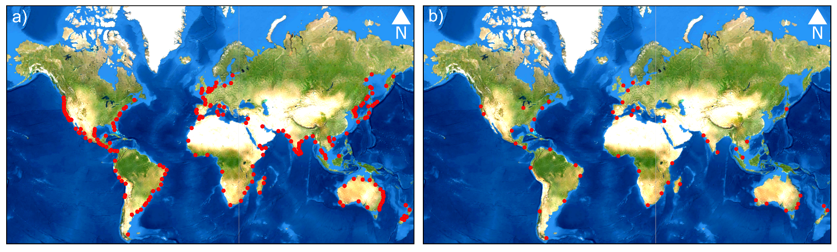
The supervised image classification—i.e., the core of the presented algorithm—needs a set of training data to work properly. We selected more than 5000 labeled points worldwide that represent sand, water, and grassy and woody vegetation through a visual inspection of Google Earth’s very high-resolution imagery for the year 2019 (see Figure 1a for the localization of the labeled points).
The algorithm works on image collections, which are sets of images acquired by the same satellite mission. We considered Sentinel-2 and Landsat images as they are freely available on the Google Earth Engine (GEE) library, but other collections can be adopted by the user once updated as a personal asset on the GEE workspace and without needing additional training points. Although Sentinel-2 and Landsat images contain multiple bands, the algorithm selects roughly half of them: the blue (B), the green (G), the red (R), the near-infrared (NIR), and the two shortwave infrared bands (SWIR1, SWIR2). In addition, the algorithm evaluates the content of the associated bitmasks (i.e., bands expressing information about quality factors through a binary codification) to apply quality filters to the images’ pixels. As the shortwave infrared bands of Sentinel-2 images have a coarser resolution (20 m) than the other bands (10 m), they are resampled to 10 m by bilinear interpolation following the methodology of similar works in the literature (e.g., [12]).
Among others, GEE generally offers two kinds of image collections: (i) top of atmosphere (TOA) images, which contain data about the whole range of light signals reflected off the Earth’s surface and travelling back through the atmosphere; (ii) surface reflectance or bottom of atmosphere (SR or BOA) images, which are derived from the post-processing of TOA to remove the noise due to light scattering and absorption by aerosols and contain only the reflectance from the Earth’s surface (see [13], for further information). We used SR images since their limited dependency on the atmospheric conditions makes them comparable in space and time, although initial tests highlight an insignificant performance difference between SR and TOA when detecting land use types in coastal areas. Further topographic corrections, accounting for incident angle and shadows, were not needed in the present case as we focused on coastal sandy areas, usually characterized by gentle slopes.
The Open Street Map (OSM) world shoreline and the Global Human Settlement Layer (GHSL), provided by the Joint Research Centre (JRC) [14], constitute the remaining input data that the algorithm demands. The GHSL is a multitemporal information layer mapping human settlements and infrastructure for the time span 1975–2014. It has been derived from satellite imagery (predominantly Landsat) and a miscellaneous dataset including census data and volunteered geographic information. The data are processed automatically using evidence-based analytics and knowledge generated from spatial data mining technologies. It has global coverage and 38 m spatial resolution and can be retrieved from the GEE’s library.
2.2. Algorithm’s Workflow
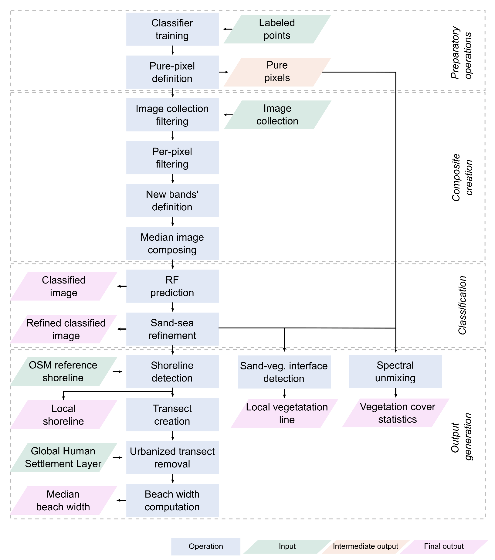
The presented algorithm was developed with the Python Application Programming Interface (API) of GEE, in order to combine GEE’s internal functions and datasets with Python libraries and the additional scripts we wrote for specific tasks. The algorithm’s workflow is graphically explained in Figure 2.
The training of the random forest (RF) classifier is the algorithm’s first step. RF is a supervised classification that ranks pixels in classes on the basis of similarity among the pixels and the spectral features of the training points. We selected the RF algorithm among the various machine learning methods that GEE makes available since it has proven to be reliable and widely used for similar applications [15,16], and does not require any particular data pre-processing prior to its implementation.
The second step consists of identifying the spectral features of the pixels representing pure sand and grass (i.e., pixels with 100% sand and grass cover, respectively). This identification relies on the labeled points taken in areas where the visual inspection indicated homogeneous cover throughout the year (see Section 2.1). The spectral features of the pure sandy pixel are computed as the median values of each spectral band in the labeled sandy points. The same method cannot be applied to the grass class because the difference between the size of the coastal vegetation patches and the spatial resolution of Landsat and Sentinel-2 images, as well as the seasonal variability of the plant biomass, hampers the identification of a pixel with 100% grass cover throughout the year. Therefore, the spectral features of the pure grassy pixel are computed as those pixels that have the highest grass biomass, indicated by the highest value of the Normalized Difference Vegetation Index (NDVI).
After these preparatory operations, the classification function starts as a loop over the various areas to be classified, hereinafter defined as areas of interest (AoIs). An image collection is generated for each AoI according to the specified time range, sensor, and surface area (see Appendix A for more details about the selection of the time range). The collection is firstly filtered according to a cloud cover threshold equal to 10%, representing a satisfying compromise between the number of selected images and their quality. Then, each image undergoes a pixel-per-pixel evaluation based on the information contained in the 8-bit mask codes. This evaluation excludes cloudy, snowy, or saturated pixels from the classification process.
Once the worst pixels are ruled out, new bands are added to the collection’s images, containing: the Modified Normalized Difference Water Index (MNDWI), the Normalized Difference Water Index (NDWI), the Enhanced Vegetation Index (EVI), the Normalized Difference Moisture Index (NDMI), and the Normalized Difference Vegetation Water Index (NDVI). The new indices are computed by applying mathematical expressions over the original image bands:
where B, G, R, , and refer to the blue, green, red, near-infrared, and shortwave infrared bands, respectively.
The RF classification is then applied to the collection’s median composite, which is the image containing the median value over time of each band in every pixel. Using median composites for image classification is very common [17,18,19,20] as it reduces the potential influence of noise and increases the number of valid observations per pixel.
Although the training dataset includes labeled water points, the sand–sea boundary classification needs to be addressed correctly. To this aim, we followed an approach commonly adopted in the literature, where a band associated with a spectral index is used to create a mask for the land and detect the shoreline (e.g., [5,9,21,22,23,24,25,26,27,28]). The selection of the most suitable spectral index to discriminate land from water is highly debated in the literature. The debate generally reduces to the comparison between the NDWI and the MNDWI, which are based on NIR and SWIR, respectively. Other indices, such as the NDVI, are usually considered less well-performing. Kelly and Gontz [7] indicate the MNDWI as the best index and several works have successfully adopted it [9,29]. Nevertheless, to the best of our knowledge, most of the literature works have preferred the NDWI so far [21,22,23,26,27,28]. As Sagar et al. [26] report, the combined use of NIR and a visible band allows for the effective detection of the waterline, despite the high environmental (and spectral) variability of intertidal zones. Furthermore, although the MNDWI is less sensitive to the white waters close to the shoreline than the NDWI [7] (the larger the wavelengths, the lower the reflectance of the white waters [8]), Ryu et al. [30] have assessed the superiority of NDWI in detecting the waterline during ebb tides and in areas characterized by high turbidity, such as shallow mudflats. Generally speaking, the MNDWI index has been developed to deal with shoreline detection in built environments and shadowed areas [22], so it is more suitable for urbanized areas, whereas NDWI is recommended for natural coastlines, such as the ones considered in the present work. Another issue widely addressed in the literature is the definition of the threshold separating the water and land classes. A large majority of the literature works set the threshold equal to 0 or to the optimal values defined by Fisher et al. [25] (e.g., −0.21 for NDWI). Although it is recognized that site-specific values would improve the accuracy of the class separation, an operator-based determination of a site-specific threshold is extremely time-consuming, especially when analyzing multiple study sites. In light of the considerations above, we set our algorithm to use the NDWI and opted for automated site-specific characterization of the threshold, in agreement with previous works (e.g., [5,9,24]). For this purpose, we followed the method proposed by Otsu [31] for image thresholding: since the histogram of the spectral index is bimodal at the sand–sea interface, with two peaks representing wet and dry pixels, respectively, the threshold is automatically chosen as the value that maximizes the separability of the two classes. As the class separability improves with the percentage of pixels occupied by water [29], the algorithm rules out those land pixels that are too far from the water and so cannot be considered belonging to the beach anymore. After the refinement of the sand–sea boundary classification, the algorithm focuses on the buffering area around the approximate shorelines provided by Open Street Map. Within this area, the local shorelines are identified and drawn applying the Canny’s edge detection operator and Hough’s transform (see [32,33], respectively, for details). Shorelines are saved according to EPSG:4326 coordinates.
In addition to land cover classification, the algorithm can compute the beach width by executing a sequence of automatic operations. Firstly, the detected shorelines are clipped within the AoI, and a set of equidistant perpendicular transects along the shorelines are created. Secondly, all the transects intersecting urban areas are removed. This operation is fundamental as the similarity between the spectral features of urban and sandy cover may lead to misclassification and jeopardize the computation of the beach extent. The presence of urban agglomerates within the AoI is evaluated by referring to the Global Human Settlement Layer (GHSL), as explained in Appendix B. Thirdly, the algorithm identifies the cover type of the pixels intersected by the transects and computes the great-circle distance d between the seaward edge of the first pixel and the landward edge of the last one by applying the Haversine formula to edges’ longitudes and latitudes [34]:
where
and R is the Earth’s radius. In the case of vegetation interrupting the sand continuum along a transect, the algorithm evaluates the extent of the vegetation patch: if the vegetation strip is narrower than 2 pixels, the algorithm includes these pixels in the beach width computation and moves landward looking for the beach edge; otherwise, it places the beach edge at the seaward side of the vegetation patch.
Eventually, the algorithm selects the grassy patched area standing behind the beach (thus excluding inland sandy areas) and computes its width along the previously created transects. It also detects the line representing the interface between the grassy area and the beach by applying Otsu’s thresholding method to the NDVI band and computes the statistics of the percentage of grass cover within the selected pixels. To this aim, the selected pixels undergo spectral unmixing, namely the identification of the percentage coverage of a specific class by referring to the spectral features of all the classes. The adoption of spectral unmixing to retrieve vegetation cover is widespread in the literature and has proven its superiority over other methods (e.g., the analysis of NDVI values [10,11]). We recall that the spectral features of the sand and grass classes have been identified at the very beginning of the algorithm through the pure pixel definition.
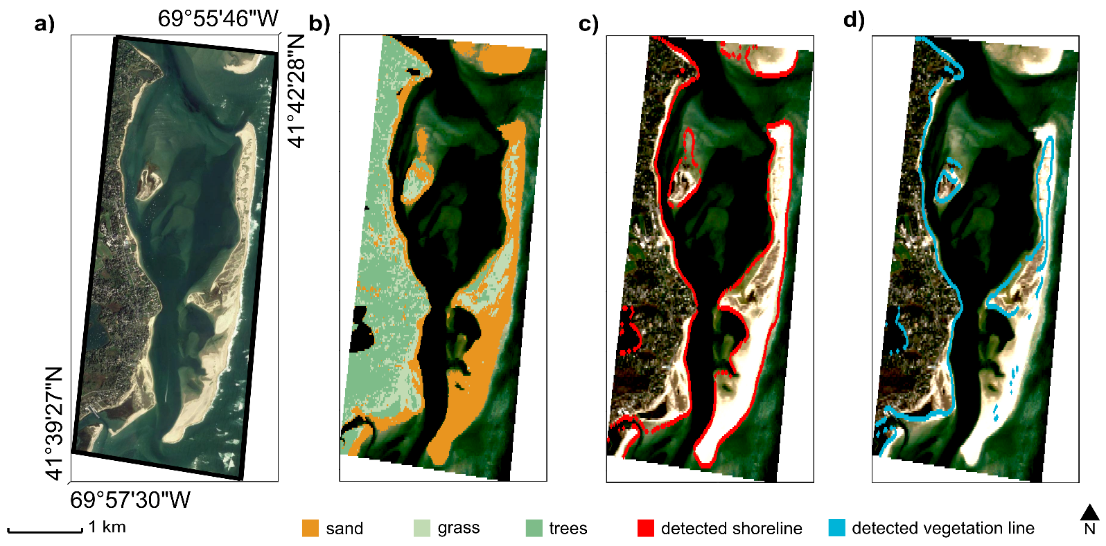
To sum up, the algorithm provides three typologies of output for a given AoI (Figure 3a): (i) the classified map of the input AoI (Figure 3b); (ii) the transition boundaries between different land cover classes as derived by combining Otsu’s threshold, Canny’s edge detection, and Hough’s transform, e.g., the shoreline (Figure 3c) and the vegetation–sand interface (Figure 3d); (iii) numeric outcomes about the transversal width of the beach and the vegetated areas, and the grass cover statistics.
2.3. Validation Methodology
RF algorithms consist of an ensemble of individual decision trees, each of these leading to a class prediction. As the final classification is the most voted class, the number of decision trees used by an RF algorithm can affect the final prediction and must be considered a parameter to be set. The size of the provided labeled-point dataset influences the prediction accuracy, too, and depends on the number of classes that must be distinguished and the intrinsic heterogeneity of the process underlying the analyzed areas.
Thus, we assessed the influence of the number of trees used by the RF algorithm and the size (i.e., the number of points) of the labeled dataset by classifying the labeled points, which were previously partitioned into training and validation subsets with a 30:70 ratio. After the classification, we estimated the associated accuracy metrics, defined as the normalized fraction of the correctly classified sample, by iterating over different couples of parameter values (dataset sizes: from 100 to 900 points per class; tree numbers: from 10 to 1000). At each iteration, we performed 100 replicates of random subsets and computed the classification accuracy. Finally, we calculated the mean and standard deviation of the accuracy for each couple of parameter values that we considered. Since the higher the standard deviation, the more inadequate the parameter setting or labeled-point dataset size, the aim was to find threshold parameters beyond which the accuracy mean (standard deviation, respectively) reaches a stable maximum (minimum). Recalling that the labeled points, here taken as ground truth, were defined according to visual inspection of very high-resolution imagery from Google Earth, this sensitivity test also provides the first quantitative validation of the classification algorithm, in agreement with similar works in the literature (e.g., [35]).
Once the optimal parameters for the RF classification were defined, we further validated the whole procedure as in Luijendijk et al. [28]. Accordingly, we randomly selected fifty areas, hereinafter referred to as areas of interest (AoIs), of approximate size 5.0 × 2.0 km all over the global shoreline. Subsequently, we visually inspected the classification results by direct comparison with very high-resolution satellite images available on Google Earth. Visual inspection is a common method to validate satellite image processing algorithms, especially when alternative datasets are missing [36]. For instance, Azzari and Lobell [35] validated Landsat-based land cover classification algorithms in GEE by determining ground truth through the visual inspection of very high-resolution imagery from Google Earth. Luijendijk et al. [28] visually validated their algorithm to classify sandy pixels over fifty beaches worldwide. Heimhuber et al. [36] defined an algorithm to study coastal inlets by processing Landsat and Sentinel-2 images and visually validated the entire imagery record across the 12 study sites. This approach allows for a fast qualitative validation at multiple sites, testing different environmental conditions, geological features (i.e., sandy composition), and numbers of available satellite images. Figure 1b shows the locations of the selected validation beaches.
Visual inspection can be affected by cognitive bias. In order to ensure a reliable accuracy estimation, we carried out a third validation of our algorithm by referring to an external dataset. This dataset was provided by Vos et al. [9] and includes 178,949 (55,673) points for Sentinel-2 (Landsat-8), subdivided into four classes (sand, water, white water, and other land features). The validation consists of evaluating the match between the real labels of the points and the classification, considering both individual classes and the overall dataset. Due to the randomness of the used classification algorithm, we carried out 100 repetitions and took the average value as the final accuracy. In this analysis, the labeled points associated with water and white water were merged prior to the validation, as our algorithm does not distinguish between these two classes.
3. Results and Discussion
3.1. Parameter Setting and First Validation
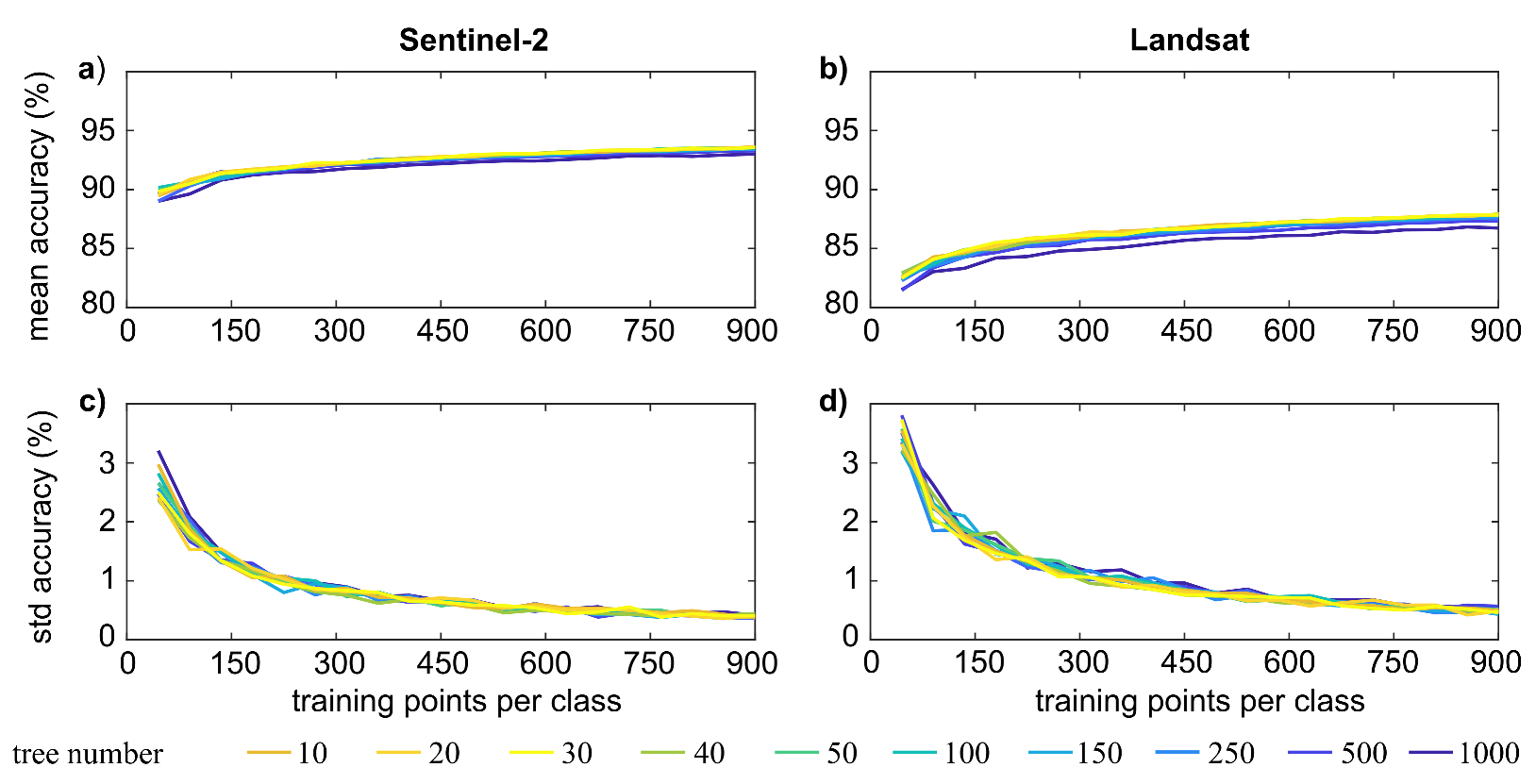
We assessed the accuracy achieved by the algorithm over both Sentinel-2 and Landsat collections. In all the tested cases, the mean and standard deviation of the accuracy reaches a constant value when each class has at least 700 points, which is much less than the number of the labeled datasets (Section 2.1). With more than 20 decision trees, the classification accuracy does not change significantly, and the optimal accuracy is achieved with 30–50 decision trees.
As Figure 4 shows, the classification over the two collections achieves excellent accuracy values for both cases, although Landsat-related results are somewhat impacted by the lower spatial resolution of the sensor’s images. In fact, whereas the standard deviation of the achieved accuracy is very low for both cases (0.5% and 0.4% for Sentinel-2 and Landsat, respectively), the mean accuracy of Sentinel-2 (93%) decisively exceeds the Landsat’s one (87%). The literature indicates that the overall accuracy can be improved by up to 4% with proper selection of the RF input features and dataset size [37]. However, we only focused on the latter aspect in this work since the determination of the best feature selection method requires a dedicated, in-depth analysis (see [38] for further details).
3.2. Second Validation across the Selected AoIs
Since Sentinel-2 has a five-day revisit time at the equator (the revisit time decreases as the latitude increases) and Landsat eigth days (considering the offset between Landsat-7 and -8), the collection of the former should contain more images than the latter. However, the cloud cover and acquisition conditions influence the number of collected images. As reported by Bergsma and Almar [39], the equator and higher latitudes have generally higher cloud coverage than mid-latitudes (i.e., around 30 degrees): at higher latitudes, the large cloud coverage might be balanced by more frequent revisits, increasing the chance of a large cloud-free collection; at the equator, instead, high cloud coverage could dramatically reduce the potential of satellite-based analyses, especially in the Gulf of Guinea and Indonesia. In this work, the number of Sentinel-2 cloud-free image collections exceeds the Landsat ones for only 58% of the selected AoIs and, regardless of the satellite mission, generally agrees with Bergsma and Almar [39]. As Figure 5a shows, mid-latitudes are associated with the largest image collections, whereas the collection size at the equator is smaller, mainly because of the relatively long revisit time. At the poles, the collection size reduces, likely due to prevailing adverse meteorological conditions, despite a very short revisit time (approximately one day).
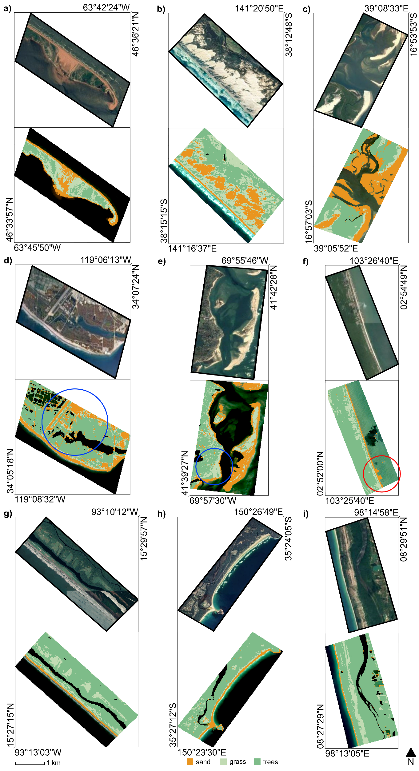
Regarding the land cover classification—i.e., one of the main outputs of the presented algorithm—a qualitative visual inspection shows the good representativeness of the identified land cover (seawater bodies, sand, grassy, and tree cover).
Sand is always well recognized when belonging to both beaches and bare inland areas (Figure 6a,b). The algorithm also classifies the sediments as sand in extended mudflats (Figure 6c).
The presence of urban areas may lead to misclassification. As aforementioned, very dense urban agglomerates usually cause commission error for the sand class, meaning that the algorithm classifies buildings and roads as sand because of their spectral resemblance (blue circle in Figure 6d). In contrast, when tree-lined boulevards or flowerbeds occupy part of the urban area, the algorithm may fail in distinguishing vegetated and urban pixels, likely because of incompatibility between the spatial scale of vegetated patches and the resolution of the satellite images (blue circle in Figure 6e). We might address this specific issue by applying spectral unmixing over urban areas, but this would slow down the algorithm without leading to a significant improvement in the study of coastal areas, which is the aim of the presented work.
Seawater is generally correctly identified if enough satellite images are available. Otherwise, the tides, together with daily to seasonal variability in wave and beach features, may influence the overall result (red circle in Figure 6f). Moreover, the availability of a few satellite images exacerbates the issue of white waters affecting shoreline detection [8], whereas the higher the number of images, the lower the noise due to individual breaking wave events.
The detection of inland water depends on several factors: tiny rivers and irrigation channels (i.e., width smaller than the pixel spatial resolution) are not recognized, whereas larger water bodies are usually correctly identified (see the different classification of the smaller and broader channels in Figure 6g). Intermediately sized water bodies are detected when surrounded by bare soils or grass and poorly recognized as tree-covered when surrounded by high and thick vegetation because of the similarity in the NDWI response (Figure 6h,i).
A summary of the algorithm’s potentialities, weaknesses, and potential solutions that the visual inspection of results has highlighted is shown in Table 1.
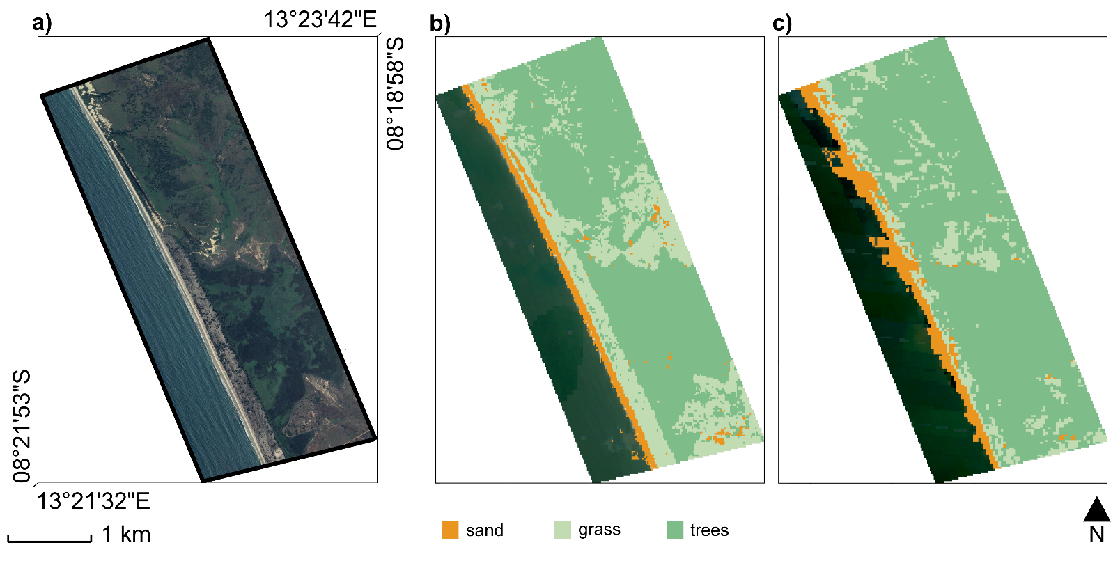
The discussed results relate to the application of the algorithm over the Sentinel-2 image collection, but similar considerations typically hold for Landsat images. Generally, Sentinel-2 allows for a more accurate classification (e.g., Figure 7), likely because of its finer spatial resolution (10 m) and shorter revisit period, which allows the collection of more images than Landsat for the same timespan.
The median beach width values are higher for Landsat image processing than for Sentinel-2 in 76% of the AoIs (Figure 5c). The mean absolute difference between the Sentinel-2-derived and Landsat-derived width values is 56 m, which is approximately double the Landsat pixel size.
The vegetation cover statistics, computed for the first row of grassy pixels that are located landward the beach, show a similar trend for Sentinel-2 and Landsat image classification (Figure 5c–f). Slight differences are likely due to the coarser resolution of Landsat images that may include non-grassy areas within its grass class because of the heterogeneity of the spatial scales of grassy patches and image pixels.
The comparison between the results obtained using Sentinel-2 and Landsat image collections highlights the consistency of the vegetation cover statistics, and the lower accuracy in the Landsat-derived classification of the sand–sea interface and computed beach widths. Slight differences in the obtained results are likely related to the different positional accuracy of the two satellite missions: the circular error at the 90th percentile is 5 m and 12 m for Sentinel-2 and Landsat-8, respectively.
3.3. Third Validation Referring to an External Dataset
As Table 2 shows, the application of the presented algorithm to an external dataset of labeled points achieved high values of the average classification accuracy for the sand and water classes but lower values for the other land features. Sentinel-2 outperformed Landsat-8 in the classification of sand (99% vs. 81%) and water (99% vs. 79%), whereas Landsat-8 showed the best performance for the other land features (40% vs. 69%) and the overall classification (59% vs. 72%). The low accuracy achieved for the other land features is due to the different labeling systems adopted by Vos et al. [9]. The present algorithm is suitable for natural beaches; it classifies sand, water, and vegetation, but it cannot distinguish between urban and non-urban land cover. Instead, the external dataset refers to sand and water and includes both vegetation and urban areas in the same class.
3.4. Multitemporal Analysis
In Section 3.2, the Sentinel-2-derived classification is shown to outperform the classification with Landsat imagery, and some methods to further improve the algorithm’s performance are mentioned. Nevertheless, it is worth noting that the 30 m Landsat spatial resolution allows us to visualize and study most of the processes occurring in natural and coastal environments, such as the detection of beach erosion and accretion trends [28], the investigation of greening or desertification processes [15], and, more generally, the identification of land cover changes in the classes labeled during the training of the classification algorithm [20]. Furthermore, it should be considered that Sentinel-2’s oldest images date back to mid-2015 only, whereas Landsat ones date back to the 1980s. Thus, Landsat image collections allow us to perform multi-annual analyses and detect historical trends and variations in each algorithm’s output despite their relatively coarser resolution. These satellite-derived time series can shed light upon the environmental dynamics occurring in coastal areas, such as bio-geomorphological time evolution.
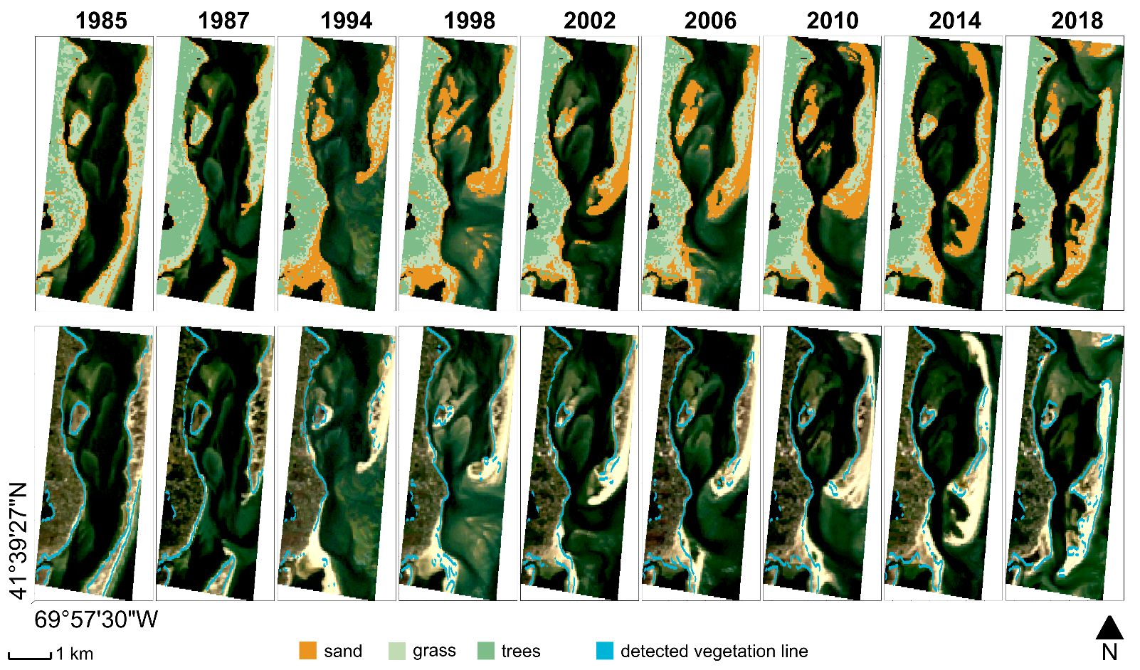
Figure 8 shows an illustrative example of time evolution analysis of a coastal site supported by Landsat image processing over one of the fifty AoIs considered for the algorithm validation. The selected site comprises part of the barrier islands in front of Chatham (Massachusetts, USA), whose morphological evolution is extensively documented by scientific studies (see [40], for further information) and press releases. The oldest images in the Landsat collection, dating up to the 1980s, show a coastal barrier protecting Chatham from the Atlantic Ocean’s flood. In 1987, a Nor’easter (a violent storm moving along the North America East Coast) cut an inlet in the barrier, generating the so-called South Beach Island. Since then, the barrier system continued to change gradually until another storm in 2007 caused a new breakage generating the North Beach Island. The annual land cover classification provided by the algorithm, which is based on aggregated images consisting of multiple images over a year (upper panels in Figure 8), highlights both the slow and abrupt changes in the barrier’s morphology. Morphological information is fundamental to understand to what extent barriers can dampen the incoming wind and wave energy and protect the mainland.
Although the main morphological and sand cover changes might be directly detected from RGB images, the algorithm offers an automated method to process the satellite images. Moreover, as it works on more bands than only RGB, it allows us to identify also those features, such as the transition line between sand and vegetation, that are not evident with the visible bands alone (lower panels in Figure 8). In the example reported in Figure 8, vegetation zonation in barrier islands generally follows the gradient that mirrors the species adaptation to salinity and resistance to floods, and significant morphological changes, such as the ones that occurred in 1987 and 2007, may dramatically alter the plant distribution and ecosystem functionality. The algorithm applied in this area may support the study of the time evolution of vegetated areas and the associated ecosystem dynamics in conjunction with the morphological shift.
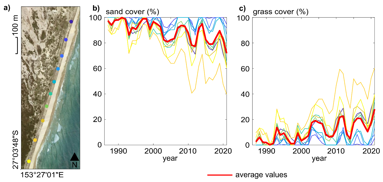
Figure 9 shows another example of time analysis supported by the application of the presented algorithm. The selected site is a subset, approximately 1000 × 500 m, of one of the fifty areas considered for the previously described validation, and it is located at Cape Moreton Conservation Park in South Eastern Australia. In this case, a visual inspection of the very high-resolution imagery available on Google Earth detects a time variation in the vegetation cover and a slight greening of the beach. However, Google Earth provides neither enough images to infer a temporal trend nor tools to compute land cover statistics to support this hypothesis. To the best of our knowledge, no quantitative datasets regarding vegetation cover are available for this area, despite its ecological relevance and the support that this kind of data may give to coastal management practices. In light of these considerations, we explored the potentialities of the presented algorithm to retrieve ecological data. For instance, we quantitatively assessed the trend of sand and vegetation cover in ten points sampled along the 2019 vegetation–sand interface. The resulting annual median land cover values for each point are displayed in Figure 9, confirming the hypothesis of seaward-moving vegetation.
We acknowledge that 10 m or 30 m resolution is insufficient to capture those local dynamics causing ecomorphological changes equal to or lower than the pixel size. Nevertheless, as mentioned in Section 2.1, the algorithm can be applied to other image datasets to meet the desired conditions of spatial resolution. For instance, it can be implemented using the products of very high-resolution commercial optical satellite missions such as GeoEye-1 (0.41 m), Worldview (0.31 to 0.46 m), Pleiades-HR (0.5 m), Kompsat-3 (0.5 m), Gaofen-2 (0.81 m), and SkySat (0.57 to 0.86 m) [41]. In addition, in the case of relying on publicly available datasets, as we did in this work, algorithm customization can enhance the performance. A first modification may consist of implementing super-resolution methods based on a deep neural network (e.g., [42]). Alternatively, sub-pixel RF classification may be carried out after downscaling or image fusion. Downscaling methods statistically convert the land cover fractions provided by the spectral unmixing in sub-pixel land cover classes. Instead, image fusion or pan-sharpening methods generally combine coarser images with panchromatic images having a finer spatial resolution. Although pan-sharpening does not increase the spatial resolution of the original image bands, it provides supplementary sub-pixel information that can support land cover classification and interface detection. Moreover, compositing a temporal sequence of NDWI layers results in sub-pixel classification for coastal changes, as demonstrated by Hagenaars et al. [6]. Despite the large availability of algorithms and functions for sub-pixel classification in GEE and the literature (e.g., [43,44]), the increase in computational time that they require must be considered. The search for increased accuracy and the best speed–accuracy trade-off is not considered in the present work and will be the object of future investigations.
4. Conclusions
The use of satellite images to investigate environmental dynamics is spreading and has already proven to be a fast and effective means of performing coarse-scale multitemporal studies. In coastal areas, satellite image processing can support the monitoring of the spatio-temporal evolution of transitional boundaries, such as the shoreline and the sand–vegetation interface. These boundaries indicate the extent of sandy beaches but also set the spatial limits for specific ecological dynamics.
With the aim to create a tool able to process satellite image collections and provide a large variety of data from coastal environments, we set up an algorithm based on Google Earth Engine (GEE) Python API. This tool combines GEE’s internal functions with supplementary scripts (e.g., shoreline identification and transect creation) to handle both GEE’s and external datasets. In the present version, the algorithm works with a user-defined image collection and can return the classified map of an area of interest according to four land cover classes (i.e., water, sand, grassy vegetation, trees). It also returns the shorelines, the vegetation–sand interface, and some numerical results about the beach width and vegetation cover statistics. The algorithm combines consolidated techniques and explores their use in coastal areas. For instance, whereas the use of thresholding methods is common for SDS, to the best of our knowledge, no other works adopt it to detect other kinds of interfaces of ecomorphological value, such as the separation between vegetation and bare ground.
We validated the algorithm through a multi-step process. Firstly, we assessed its performance by computing the accuracy statistics over a set of manually labeled points. Secondly, we performed a visual inspection of fifty areas of interest (AoIs). Both the manually labeled points and the AoIs were randomly chosen worldwide, so that the algorithm deals with varying image collection features (in terms of both number and quality of the contained images), different latitudes, and a large variety of geological and hydraulic conditions. We applied the algorithm over either Sentinel-2 or Landsat image collections, achieving high classification accuracy (90% on average). The comparison between these two sensors highlighted the consistency of the obtained vegetation cover statistics but the slightly lower classification accuracy for the Landsat case (87% versus 93%) because of its coarser spatial image resolution. Thirdly, we provided a quantitative validation by assessing the classification accuracy over the labeled points belonging to an external dataset. The obtained accuracy for the classes considered by our algorithm and the external dataset (i.e., water and sand) were higher for Sentinel-2 than Landsat-8 (99% versus 80% on average). All the validation tests that we carried out highlight the slightly lower accuracy for the classification over Landsat imagery than Sentinel-2. Nevertheless, we observed the crucial role of Landsat collections to study temporal dynamics and provided two examples about their potential use to define the time series of land cover changes and other variables.
The algorithm validation relies on the visual inspection of results. As aforementioned in Section 3.2, this method is commonly adopted in similar applications to carry out multiple-site, low-cost validations and does not require high technical qualifications. Nevertheless, visual inspection also has some drawbacks that must be considered when evaluating its results, such as the potential misinterpretation of the reference land cover, the missing of minor inaccuracies, and the bias related to the inspector’s experience. In light of these considerations, we acknowledge that the validation would have benefited from in situ measurements. However, field campaigns for this kind of application are highly complex and costly, as they would require measurements across several sites, preferably located in different regions worldwide, repeated over time. To address this issue, the following works will focus on field measurements and the local application of the algorithm, setting the basis for a shared database of land cover and coastal data to support the new satellite image processing algorithms to come.
We sum up by remarking that satellite image processing typically requires large memory and computational capability from the user (i.e., the client side), limiting the spatial and temporal bounds of the analysis. To avoid these constraints, we developed the presented algorithm to handle satellite images through free online computing platforms. In this way, the image collections and most of the intermediate variables are never downloaded by the client, and the functions run by leveraging cloud-based parallelized computing. The client-side resources are used only to export the final output and carry out a few other basic operations. Combining the user’s independence from personal computational capability and the good classification performance at different locations worldwide, the presented algorithm has potential for global scaling. Moreover, it is versatile and can be further customized to provide the desired output. Finally, it can be used to gather useful information for scholars and land managers about ecological and morphological trends in a fast and robust manner for any beach worldwide, from a local to continental and global scale.
Supplementary Materials
The following are available at https://www.mdpi.com/article/10.3390/rs13224613/s1: a folder containing the labeled point datasets and the documents with the indications to run the algorithm.
Author Contributions
Conceptualization, A.L., C.C., and M.L.; methodology and software, A.L., A.M.M.-R., and M.L.; data curation, formal analysis, validation, and visualization, M.L.; writing—original draft preparation, M.L.; review and editing, A.L., A.M.M.-R., C.C., and M.L. All authors have read and agreed to the published version of the manuscript.
Funding
This research was partly funded by the Deltares Strategic Research Programme Seas and Coastal Zones.
Institutional Review Board Statement
Not applicable.
Informed Consent Statement
Not applicable.
Data Availability Statement
The satellite imagery that were analyzed in this study were derived from publicly available datasets. The Sentinel-2 and Landsat image collections can be freely downloaded from the Google Earth Engine dataset at https://developers.google.com/earth-engine/datasets, accessed on 30 August 2021. The algorithm presented in this study is available upon request from the corresponding author.
Acknowledgments
We would like to acknowledge Josh Friedman for his contributions during his time at Deltares, particularly in relation to the automated image collection and the shoreline detection.
Conflicts of Interest
The authors declare no conflict of interest.
Abbreviations
The following abbreviations are used in this manuscript:
| AoI | Area of Interest |
| API | Application Programming Interface |
| BOA | Bottom of Atmosphere |
| EVI | Enhanced Vegetation Index |
| GEE | Google Earth Engine |
| GHSL | Global Human Settlement Layer |
| JRC | Joint Research Center |
| MNDWI | Modified Normalized Difference Water Index |
| NDMI | Normalized Difference Moisture Index |
| NDVI | Normalized Difference Vegetation Index |
| NDWI | Normalized Difference Water Index |
| NIR | Near-Infrared |
| OSM | Open Street Map |
| RF | Random Forest |
| RGB | Red–Green–Blue |
| SDS | Satellite-Derived Shoreline |
| SR | Surface Reflectance |
| SWIR | Shortwave Infrared |
| TOA | Top of Atmosphere |
Appendix A. Setting the Time Range for Image Gathering
When dealing with vegetation, referring to growing seasons allows for a better classification than senescence or dormant seasonal periods [15,45], as this may avoid the incorrect inclusion of sandy pixels in the grass class. More generally, grouping the images according to their season can improve the preservation of explicit phenological information [35]. The time range for image gathering is an input parameter of the algorithm and can be adjusted to capture those periods when the NDVI, which is a proxy of vegetation biomass [46], shows a plateau around its maximum value, indicating the season of higher photosynthetic activity. Nevertheless, matching satellite-based phenology with site-specific plant phenophases would require extensive field surveys and is strongly hampered by both spatial and temporal scale incompatibility [47].
Our algorithm does not aim to discriminate plant classes but to provide a coarse-scale extension of the vegetated area. Therefore, we set it to collect images throughout the year, thus reducing the influence of image noise and low-quality pixels and allowing for worldwide application without prior site-specific knowledge of the growing season and vegetation features.
Appendix B. Removing the Urbanized Transects
The Global Human Settlement Layer (GHSL) aims to represent urbanized areas. We performed a visual inspection to determine the correspondence between the GHSL’s urban pixels and the real urbanized areas. It was found that the largest agglomerates are well-represented by GHSL. Nevertheless, the GHSL often misclassifies beaches, labeling them as urban, and this is likely due to the spectral similarity between sands and building materials, as mentioned in Section 2.2. Moreover, the GHSL shows poor precision for the narrowest anthropic infrastructures, such as streets, likely because of the 30 m spatial scale of its underlying Landsat data.
These local inaccuracies, despite being negligible for some applications, may impact the definition of the beach boundaries and the computation of its width. Therefore, we decided to process the GHSL before evaluating the potential intersection between it and the transects. We firstly computed the degree of connections among pixels in order to define clusters, and then we selected all those clusters greater than 25 ha, obtaining a layer representing towns and cities only.
An example of the GHSL processing and the removal of urbanized transects is shown in Figure A1.
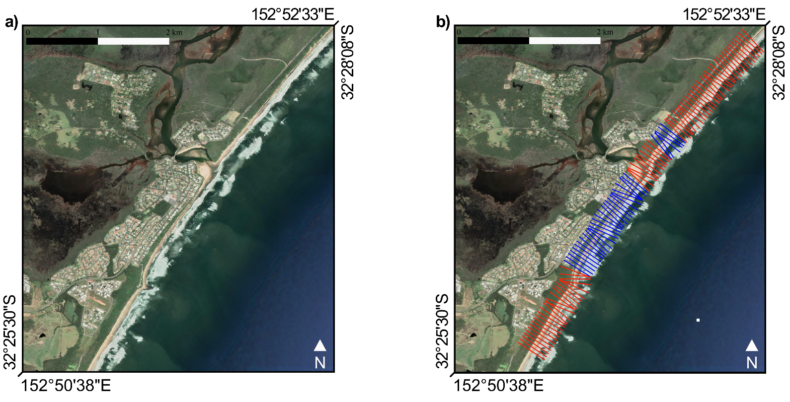
Figure A1.
For selected areas of interest (a), the algorithm creates a set of transects perpendicular to the detected shoreline (b) and evaluates whether they intersect urban agglomerates (in blue) or not (in red) (EPSG:4326).
Figure A1.
For selected areas of interest (a), the algorithm creates a set of transects perpendicular to the detected shoreline (b) and evaluates whether they intersect urban agglomerates (in blue) or not (in red) (EPSG:4326).

References
- Small, C.; Nicholls, R.J. A Global Analysis of Human Settlement in Coastal Zones. J. Coast. Res. 2003, 19, 584–599. [Google Scholar]
- Hallegate, S.; Green, C.; Nicholls, R.J.; Corfee-Morlot, J. Future flood losses in major coastal cities. Nat. Clim. Chang. 2013, 3, 802–806. [Google Scholar] [CrossRef]
- Hinkel, J.; Nicholls, R.J.; Tol, R.S.; Wang, Z.B.; Hamilton, J.M.; Boot, G.; Vafeidis, A.T.; McFadden, L.; Ganopolski, A.; Klein, R.J. A global analysis of erosion of sandy beaches and sea-level rise: An application of DIVA. Glob. Planet. Chang. 2013, 111, 150–158. [Google Scholar] [CrossRef]
- SEDAC. Percentage of Total Population Living in Coastal Areas; Socioeconomic Data and Applications Center: Columbia, SC, USA, 2011.
- Choung, Y.J.; Jo, M.H. Shoreline change assessment for various types of coasts using multi-temporal Landsat imagery of the east coast of South Korea. Remote Sens. Lett. 2016, 7, 91–100. [Google Scholar] [CrossRef]
- Hagenaars, G.; de Vries, S.; Luijendijk, A.P.; de Boer, W.P.; Reniers, A.J. On the accuracy of automated shoreline detection derived from satellite imagery: A case study of the sand motor mega-scale nourishment. Coast. Eng. 2018, 133, 113–125. [Google Scholar] [CrossRef]
- Kelly, J.T.; Gontz, A.M. Using GPS-surveyed intertidal zones to determine the validity of shorelines automatically mapped by Landsat water indices. Int. J. Appl. Earth Obs. Geoinf. 2018, 65, 92–104. [Google Scholar] [CrossRef]
- Pardo-Pascual, J.E.; Sánchez-García, E.; Almonacid-Caballer, J.; Palomar-Vázquez, J.M.; Priego De Los Santos, E.; Fernández-Sarría, A.; Balaguer-Beser, Á. Assessing the accuracy of automatically extracted shorelines on microtidal beaches from Landsat 7, Landsat 8 and Sentinel-2 imagery. Remote Sens. 2018, 10, 326. [Google Scholar] [CrossRef] [Green Version]
- Vos, K.; Splinter, K.D.; Harley, M.D.; Simmons, J.A.; Turner, I.L. CoastSat: A Google Earth Engine-enabled Python toolkit to extract shorelines from publicly available satellite imagery. Environ. Model. Softw. 2019, 122, 104528. [Google Scholar] [CrossRef]
- Elmore, A.J.; Mustard, J.F.; Manning, S.J.; Lobell, D.B. Quantifying vegetation change in semiarid environments: Precision and accuracy of spectral mixture analysis and the normalized difference vegetation index. Remote Sens. Environ. 2000, 73, 87–102. [Google Scholar] [CrossRef]
- Hostert, P.; Röder, A.; Hill, J. Coupling spectral unmixing and trend analysis for monitoring of long-term vegetation dynamics in Mediterranean rangelands. Remote Sens. Environ. 2003, 87, 183–197. [Google Scholar] [CrossRef]
- Traganos, D.; Reinartz, P. Machine learning-based retrieval of benthic reflectance and Posidonia oceanica seagrass extent using a semi-analytical inversion of Sentinel-2 satellite data. Int. J. Remote Sens. 2018, 39, 9428–9452. [Google Scholar] [CrossRef]
- Medina-Lopez, E. Machine Learning and the End of Atmospheric Corrections: A Comparison between High-Resolution Sea Surface Salinity in Coastal Areas from Top and Bottom of Atmosphere Sentinel-2 Imagery. Remote Sens. 2020, 12, 2924. [Google Scholar] [CrossRef]
- Pesaresi, M.; Ehrlich, D.; Florczyk, A.J.; Freire, S.; Julea, A.; Kemper, T.; Soille, P.; Syrris, V. GHS Built-Up Datamask Grid Derived from Landsat, Multitemporal (1975, 1990, 2000, 2014A [Dataset]. 2015. Available online: https://data.europa.eu/89h/jrc-ghsl-ghs_built_ldsmtdm_globe_r2015b (accessed on 20 March 2021).
- Hansen, M.C.; Potapov, P.V.; Moore, R.; Hancher, M.; Turubanova, S.A.; Tyukavina, A.; Thau, D.; Stehman, S.; Goetz, S.J.; Loveland, T.R.; et al. High-resolution global maps of 21st-century forest cover change. Science 2013, 342, 850–853. [Google Scholar] [CrossRef] [Green Version]
- Marzialetti, F.; Giulio, S.; Malavasi, M.; Sperandii, M.G.; Acosta, A.T.R.; Carranza, M.L. Capturing coastal dune natural vegetation types using a phenology-based mapping approach: The potential of Sentinel-2. Remote Sens. 2019, 11, 1506. [Google Scholar] [CrossRef] [Green Version]
- Miettinen, J.; Shi, C.; Liew, S.C. Land cover distribution in the peatlands of Peninsular Malaysia, Sumatra and Borneo in 2015 with changes since 1990. Glob. Ecol. Conserv. 2016, 6, 67–78. [Google Scholar] [CrossRef] [Green Version]
- Wingate, V.R.; Phinn, S.R.; Kuhn, N.; Bloemertz, L.; Dhanjal-Adams, K.L. Mapping decadal land cover changes in the woodlands of north eastern Namibia from 1975 to 2014 using the Landsat satellite archived data. Remote Sens. 2016, 8, 681. [Google Scholar] [CrossRef] [Green Version]
- Oliphant, A.J.; Thenkabail, P.S.; Teluguntla, P.; Xiong, J.; Gumma, M.K.; Congalton, R.G.; Yadav, K. Mapping cropland extent of Southeast and Northeast Asia using multi-year time-series Landsat 30-m data using a random forest classifier on the Google Earth Engine Cloud. Int. J. Appl. Earth Obs. Geoinf. 2019, 81, 110–124. [Google Scholar] [CrossRef]
- Xie, S.; Liu, L.; Zhang, X.; Yang, J.; Chen, X.; Gao, Y. Automatic land-cover mapping using Landsat time-series data based on Google Earth Engine. Remote Sens. 2019, 11, 3023. [Google Scholar] [CrossRef] [Green Version]
- Murray, N.J.; Phinn, S.R.; Clemens, R.S.; Roelfsema, C.M.; Fuller, R.A. Continental scale mapping of tidal flats across East Asia using the Landsat archive. Remote Sens. 2012, 4, 3417–3426. [Google Scholar] [CrossRef] [Green Version]
- Rokni, K.; Ahmad, A.; Selamat, A.; Hazini, S. Water feature extraction and change detection using multitemporal Landsat imagery. Remote Sens. 2014, 6, 4173–4189. [Google Scholar] [CrossRef] [Green Version]
- Dhanjal-Adams, K.L.; Hanson, J.O.; Murray, N.J.; Phinn, S.R.; Wingate, V.R.; Mustin, K.; Lee, J.R.; Allan, J.R.; Cappadonna, J.L.; Studds, C.E.; et al. The distribution and protection of intertidal habitats in Australia. Emu-Austral Ornithol. 2016, 116, 208–214. [Google Scholar] [CrossRef] [Green Version]
- Donchyts, G.; Baart, F.; Winsemius, H.; Gorelick, N.; Kwadijk, J.; Van De Giesen, N. Earth’s surface water change over the past 30 years. Nat. Clim. Chang. 2016, 6, 810–813. [Google Scholar] [CrossRef]
- Fisher, A.; Flood, N.; Danaher, T. Comparing Landsat water index methods for automated water classification in eastern Australia. Remote Sens. Environ. 2016, 175, 167–182. [Google Scholar] [CrossRef]
- Sagar, S.; Roberts, D.; Bala, B.; Lymburner, L. Extracting the intertidal extent and topography of the Australian coastline from a 28 year time series of Landsat observations. Remote Sens. Environ. 2017, 195, 153–169. [Google Scholar] [CrossRef]
- Fan, Y.; Chen, S.; Zhao, B.; Pan, S.; Jiang, C.; Ji, H. Shoreline dynamics of the active Yellow River delta since the implementation of Water-Sediment Regulation Scheme: A remote-sensing and statistics-based approach. Estuar. Coast. Shelf Sci. 2018, 200, 406–419. [Google Scholar] [CrossRef]
- Luijendijk, A.; Hagenaars, G.; Ranasinghe, R.; Baart, F.; Donchyts, G.; Aarninkhof, S. The state of the world’s beaches. Sci. Rep. 2018, 8, 6641. [Google Scholar] [CrossRef]
- Donchyts, G.; Schellekens, J.; Winsemius, H.; Eisemann, E.; Van de Giesen, N. A 30 m resolution surface water mask including estimation of positional and thematic differences using Landsat 8, SRTM and OpenStreetMap: A case study in the Murray-Darling Basin, Australia. Remote Sens. 2016, 8, 386. [Google Scholar] [CrossRef] [Green Version]
- Ryu, J.H.; Won, J.S.; Min, K.D. Waterline extraction from Landsat TM data in a tidal flat: A case study in Gomso Bay, Korea. Remote Sens. Environ. 2002, 83, 442–456. [Google Scholar] [CrossRef]
- Otsu, N. A threshold selection method from gray-level histograms. IEEE Trans. Syst. Man Cybern. 1979, 9, 62–66. [Google Scholar] [CrossRef] [Green Version]
- Canny, J. A computational approach to edge detection. IEEE Trans. Pattern Anal. Mach. Intell. 1986, 679–698. [Google Scholar] [CrossRef]
- Hart, P.E.; Duda, R. Use of the Hough transformation to detect lines and curves in pictures. Commun. ACM 1972, 15, 11–15. [Google Scholar]
- Sinnott, R.W. Virtues of the Haversine. Sky Telesc. 1984, 68, 158. [Google Scholar]
- Azzari, G.; Lobell, D. Landsat-based classification in the cloud: An opportunity for a paradigm shift in land cover monitoring. Remote Sens. Environ. 2017, 202, 64–74. [Google Scholar] [CrossRef]
- Heimhuber, V.; Vos, K.; Fu, W.; Glamore, W. InletTracker: An open-source Python toolkit for historic and near real-time monitoring of coastal inlets from Landsat and Sentinel-2. Geomorphology 2021, 389, 107830. [Google Scholar] [CrossRef]
- Kiala, Z.; Mutanga, O.; Odindi, J.; Peerbhay, K. Feature Selection on Sentinel-2 Multispectral Imagery for Mapping a Landscape Infested by Parthenium Weed. Remote Sens. 2019, 11, 1892. [Google Scholar] [CrossRef] [Green Version]
- Chandrashekar, G.; Sahin, F. A survey on feature selection methods. Comput. Electr. Eng. 2014, 40, 16–28. [Google Scholar] [CrossRef]
- Bergsma, E.W.; Almar, R. Coastal coverage of ESA’Sentinel 2 mission. Adv. Space Res. 2020, 65, 2636–2644. [Google Scholar] [CrossRef]
- Borrelli, M.; Giese, G.S.; Keon, T.L.; Legare, B.; Smith, T.L.; Adams, M.; Mague, S.T. Monitoring tidal inlet dominance shifts in a cyclically migrating barrier beach system. In Coastal Sediments 2019: Proceedings of the 9th International Conference; World Scientific: Petersburg, FL, USA, 2019; pp. 1936–1944. [Google Scholar]
- Turner, I.L.; Harley, M.D.; Almar, R.; Bergsma, E.W. Satellite optical imagery in Coastal Engineering. Coast. Eng. 2021, 167, 103919. [Google Scholar] [CrossRef]
- Lanaras, C.; Bioucas-Dias, J.; Galliani, S.; Baltsavias, E.; Schindler, K. Super-resolution of Sentinel-2 images: Learning a globally applicable deep neural network. ISPRS J. Photogramm. Remote Sens. 2018, 146, 305–319. [Google Scholar] [CrossRef] [Green Version]
- Ha, W.; Gowda, P.H.; Howell, T.A. A review of downscaling methods for remote sensing-based irrigation management: Part I. Irrig. Sci. 2013, 31, 831–850. [Google Scholar] [CrossRef]
- Ha, W.; Gowda, P.H.; Howell, T.A. A review of potential image fusion methods for remote sensing-based irrigation management: Part II. Irrig. Sci. 2013, 31, 851–869. [Google Scholar] [CrossRef]
- Tucker, C.J.; Grant, D.M.; Dykstra, J.D. NASA’s global orthorectified Landsat data set. Photogramm. Eng. Remote Sens. 2004, 70, 313–322. [Google Scholar] [CrossRef] [Green Version]
- Pettorelli, N.; Vik, J.O.; Mysterud, A.; Gaillard, J.M.; Tucker, C.J.; Stenseth, N.C. Using the satellite-derived NDVI to assess ecological responses to environmental change. Trends Ecol. Evol. 2005, 20, 503–510. [Google Scholar] [CrossRef] [PubMed]
- Tomaselli, V.; Adamo, M.; Veronico, G.; Sciandrello, S.; Tarantino, C.; Dimopoulos, P.; Medagli, P.; Nagendra, H.; Blonda, P. Definition and application of expert knowledge on vegetation pattern, phenology, and seasonality for habitat mapping, as exemplified in a Mediterranean coastal site. Plant Biosyst. Int. J. Deal. All Asp. Plant Biol. 2017, 151, 887–899. [Google Scholar] [CrossRef] [Green Version]
Figure 1.
(a) Location of the manually labeled points used for the calibration and the first validation of the classification algorithm (red dots). (b) Location of the fifty selected areas of interest for the second validation of the algorithm (red dots).
Figure 1.
(a) Location of the manually labeled points used for the calibration and the first validation of the classification algorithm (red dots). (b) Location of the fifty selected areas of interest for the second validation of the algorithm (red dots).

Figure 2.
Algorithm’s workflow to classify satellite images and provide relevant information about coastal areas. Green boxes represent input, blue boxes represent operations, whereas orange and pink boxes represent intermediate and final output, respectively.
Figure 2.
Algorithm’s workflow to classify satellite images and provide relevant information about coastal areas. Green boxes represent input, blue boxes represent operations, whereas orange and pink boxes represent intermediate and final output, respectively.

Figure 3.
An example of the algorithm’s output: (a) view of the area of interest (Google Earth, 2021); (b) classified map of sand (orange), grassy vegetation (light green), and trees (dark green); (c) locally detected shorelines (in red), and (d) the vegetation–sand interfaces (cyan) (EPSG: 4326).
Figure 3.
An example of the algorithm’s output: (a) view of the area of interest (Google Earth, 2021); (b) classified map of sand (orange), grassy vegetation (light green), and trees (dark green); (c) locally detected shorelines (in red), and (d) the vegetation–sand interfaces (cyan) (EPSG: 4326).

Figure 4.
Mean and standard deviation (std) of the accuracy for increasing number of training points when the classification relies on Sentinel-2 (a,c) or Landsat (b,d) images.
Figure 4.
Mean and standard deviation (std) of the accuracy for increasing number of training points when the classification relies on Sentinel-2 (a,c) or Landsat (b,d) images.

Figure 5.
(a) Image collection size versus latitude for Landsat (blue dots) and Sentinel-2 (red dots). (b) Comparison between the Landsat- and Sentinel-2-derived median beach width (reported in meters). The main vegetation cover statistics expressed as a percentage: (c) median; (d) mean; (e) standard deviation; and (f) coefficient of variation.

Figure 6.
Comparison between very high-resolution satellite images from Google Maps and the classification based on Sentinel-2 for a selection of AoIs (EPSG: 4326): (a) New Bedford, MA, USA; (b) Discovery Bay Coastal Park, Australia; (c) Moebase, Mozambique; (d) Point Mugu, CA, USA; (e) Chatam, MA, USA; (f) Kuala Rompin, Malaysia; (g) El Palmarcito, Mexico; (h) Shoalhaven, Australia; (i) Lampi–Hat Thai Mueang National Park, Thailand. The blue circles in the panels (d,e) indicate urbanized areas, whereas the red circles in the panel (f) indicate misclassification of the sand–sea interface.

Figure 7.
Comparison between (a) the very high-resolution satellite images for a selected AoI from Google Maps and the classification based on Sentinel-2 (b) and Landsat (c) images (EPSG: 4326). The comparison clearly highlights the higher accuracy of the Sentinel-2-derived classification.
Figure 7.
Comparison between (a) the very high-resolution satellite images for a selected AoI from Google Maps and the classification based on Sentinel-2 (b) and Landsat (c) images (EPSG: 4326). The comparison clearly highlights the higher accuracy of the Sentinel-2-derived classification.

Figure 8.
Time evolution of the coastal barrier protecting the city of Chatham (Massachusetts, USA). The classified images in the upper row of panels show the land cover changes and highlight the geomorphological evolution of the area, whereas the cyan lines in the lower row of panels show the evolution of the vegetation–sand interface (EPSG: 4326).

Figure 9.
(a) Localization of ten points along the vegetation–sand interface at Cape Moreton (SE Australia) (Google Earth, 2021). Trend of sand (b) and grass (c) cover dynamics across the Landsat timespan. The line colors in the panels (b,c) refer to the point location indicated in the panel (a); the red lines show the average trend.


Table 1.
Main features of the algorithm as highlighted by the visual inspection of results.
| Potentialities | Weaknesses | Solutions |
|---|---|---|
| Good classification of sand, grass, trees, water. | ||
| Good performance at every latitude. | ||
| Satisfactory performance with few images. Application to single or multi-annual analysis. | The lower the number of images, the higher the influence of spectral and environmental noise. | Merging of different image collections. |
| Good masking of sea and freshwater. | Thick vegetation may hamper inland water masking. | Combined use of water- and vegetation-related indices to mask. |
| Beach width computation not influenced by the presence of urban areas. | Very dense urban areas classified as sand. | Use of other kinds of data to mask out cities before the classification. |
| Urban areas with flowerbeds and tree-lined boulevards classified as vegetation. | Use of spectral unmixing. |
Table 2.
Classification accuracy for the application of the presented algorithm in the dataset by Vos et al. [9].
Table 2.
Classification accuracy for the application of the presented algorithm in the dataset by Vos et al. [9].
| Class | Sentinel-2 | Landsat-8 | ||
|---|---|---|---|---|
| Points | Accuracy (%) | Points | Accuracy (%) | |
| Sand | 4842 | 99 | 7009 | 81 |
| Water | 51,920 | 99 | 18,513 | 79 |
| White water | 2142 | 752 | ||
| Other land features | 120,045 | 40 | 29,399 | 69 |
| Overall | 178,949 | 59 | 55,673 | 72 |
Publisher’s Note: MDPI stays neutral with regard to jurisdictional claims in published maps and institutional affiliations. |
© 2021 by the authors. Licensee MDPI, Basel, Switzerland. This article is an open access article distributed under the terms and conditions of the Creative Commons Attribution (CC BY) license (https://creativecommons.org/licenses/by/4.0/).
Share and Cite
MDPI and ACS Style
Latella, M.; Luijendijk, A.; Moreno-Rodenas, A.M.; Camporeale, C. Satellite Image Processing for the Coarse-Scale Investigation of Sandy Coastal Areas. Remote Sens. 2021, 13, 4613. https://doi.org/10.3390/rs13224613
AMA Style
Latella M, Luijendijk A, Moreno-Rodenas AM, Camporeale C. Satellite Image Processing for the Coarse-Scale Investigation of Sandy Coastal Areas. Remote Sensing. 2021; 13(22):4613. https://doi.org/10.3390/rs13224613
Chicago/Turabian StyleLatella, Melissa, Arjen Luijendijk, Antonio M. Moreno-Rodenas, and Carlo Camporeale. 2021. "Satellite Image Processing for the Coarse-Scale Investigation of Sandy Coastal Areas" Remote Sensing 13, no. 22: 4613. https://doi.org/10.3390/rs13224613
Note that from the first issue of 2016, this journal uses article numbers instead of page numbers. See further details here.