
Accuracy Evaluation on Geolocation of the Chinese First Polar Microsatellite (Ice Pathfinder) Imagery

 ,
,  , , and
Abstract
:
1. Introduction
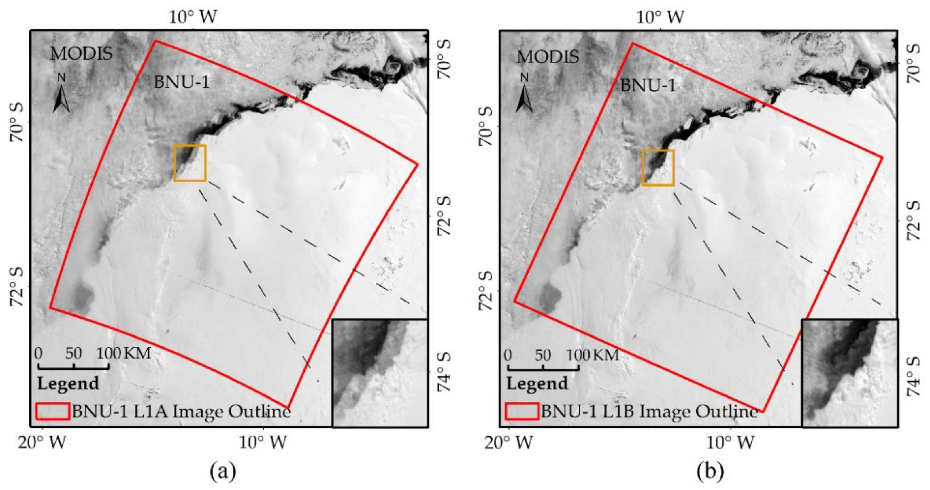
2. Data
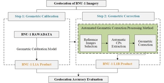
3. Methods
3.1. Geometric Calibration Model
3.1.1. Description of Geometric Calibration Model
3.1.2. Uncertainty Evaluation of Geometric Calibration Model
3.2. Automated Geometric Correction Processing Method
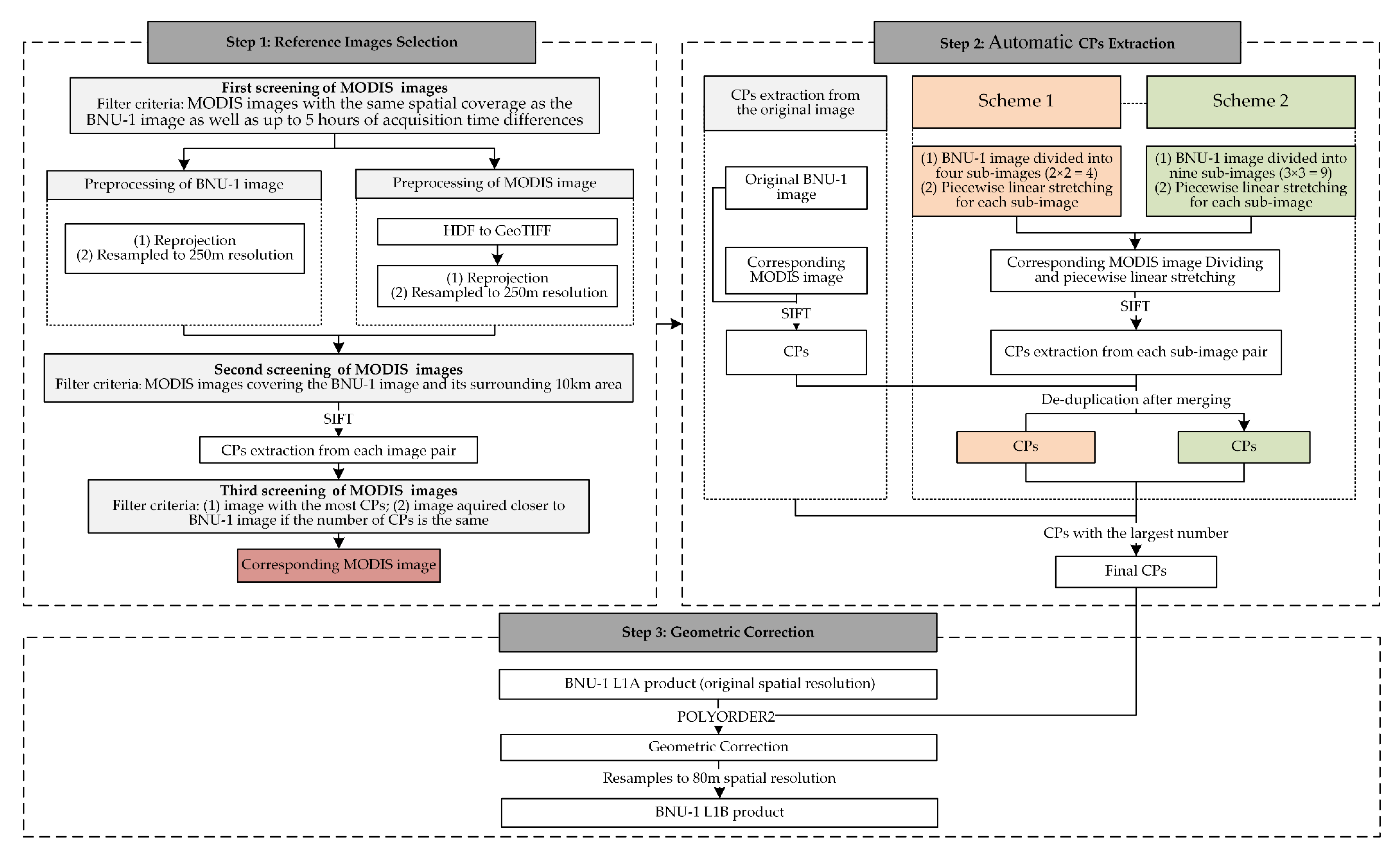
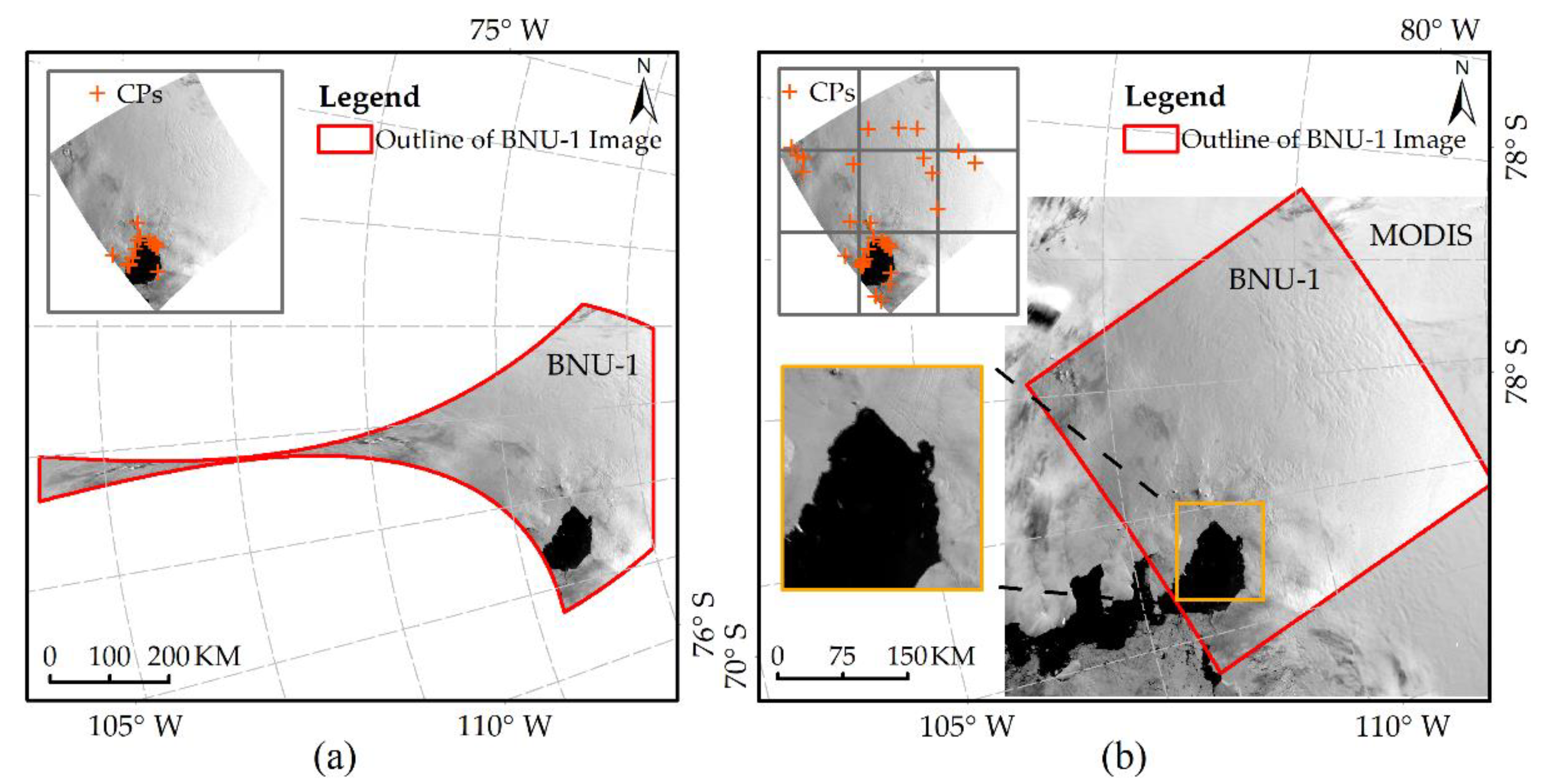
3.2.1. Step 1: Reference Images Selection
3.2.2. Step 2: Automatic CPs Extraction
3.2.3. Step 3: Geometric Correction
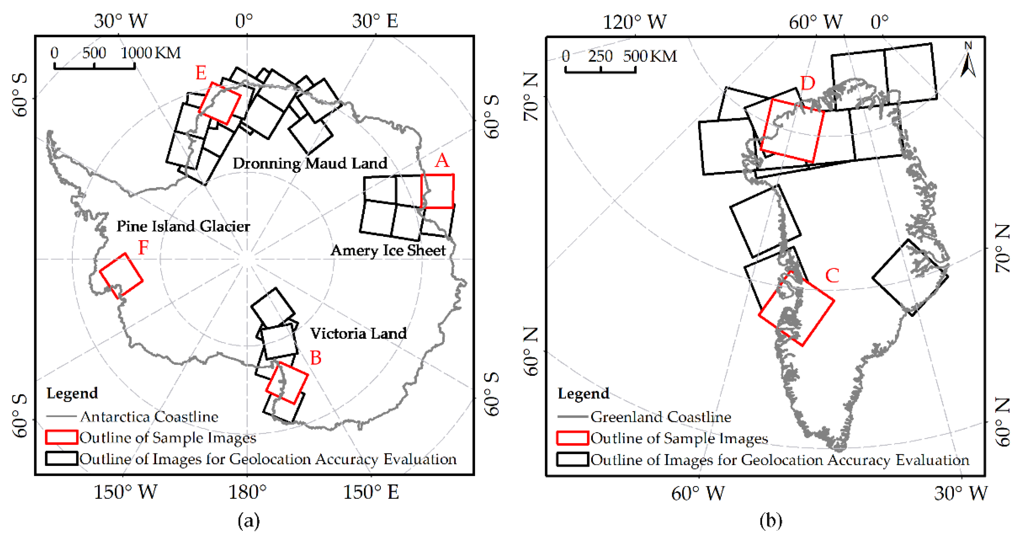
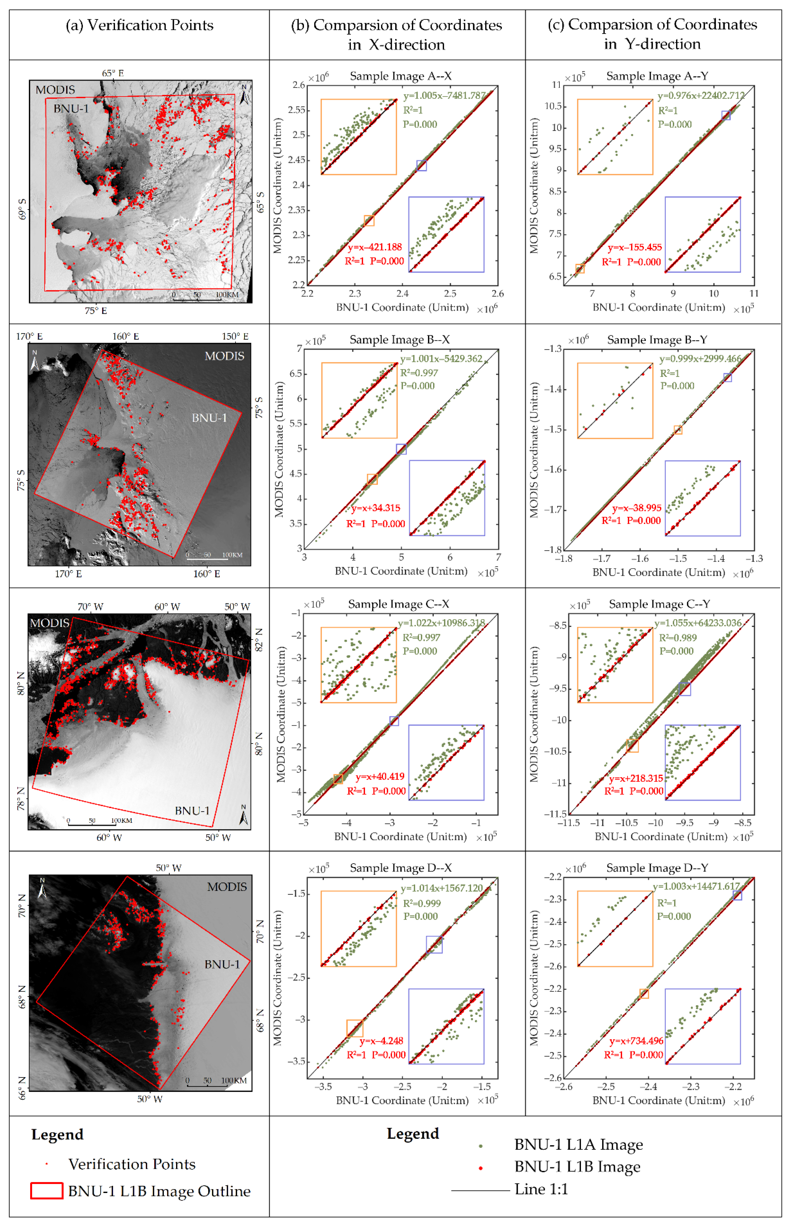
3.3. Geolocation Accuracy Evaluation
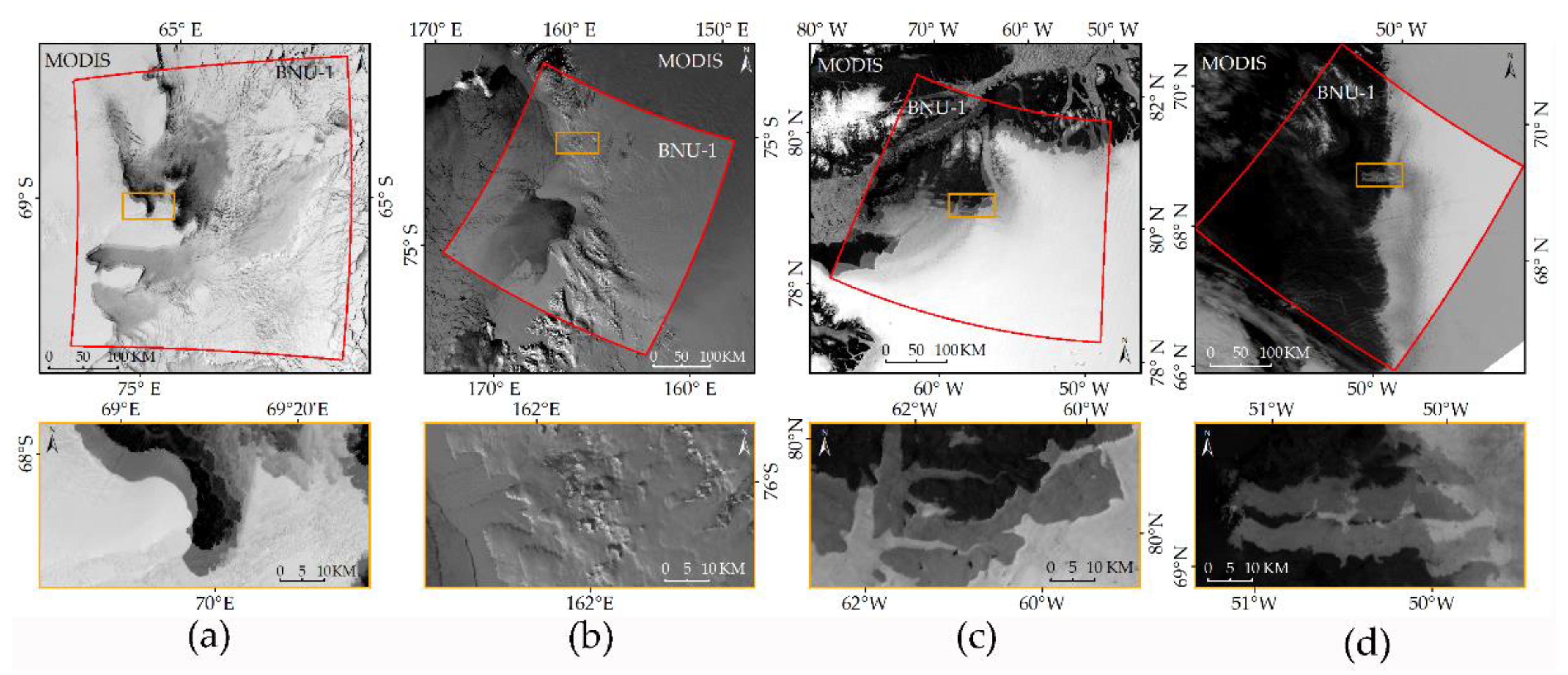
4. Results
4.1. Geolocation Accuracy of the BNU-1 L1A Product
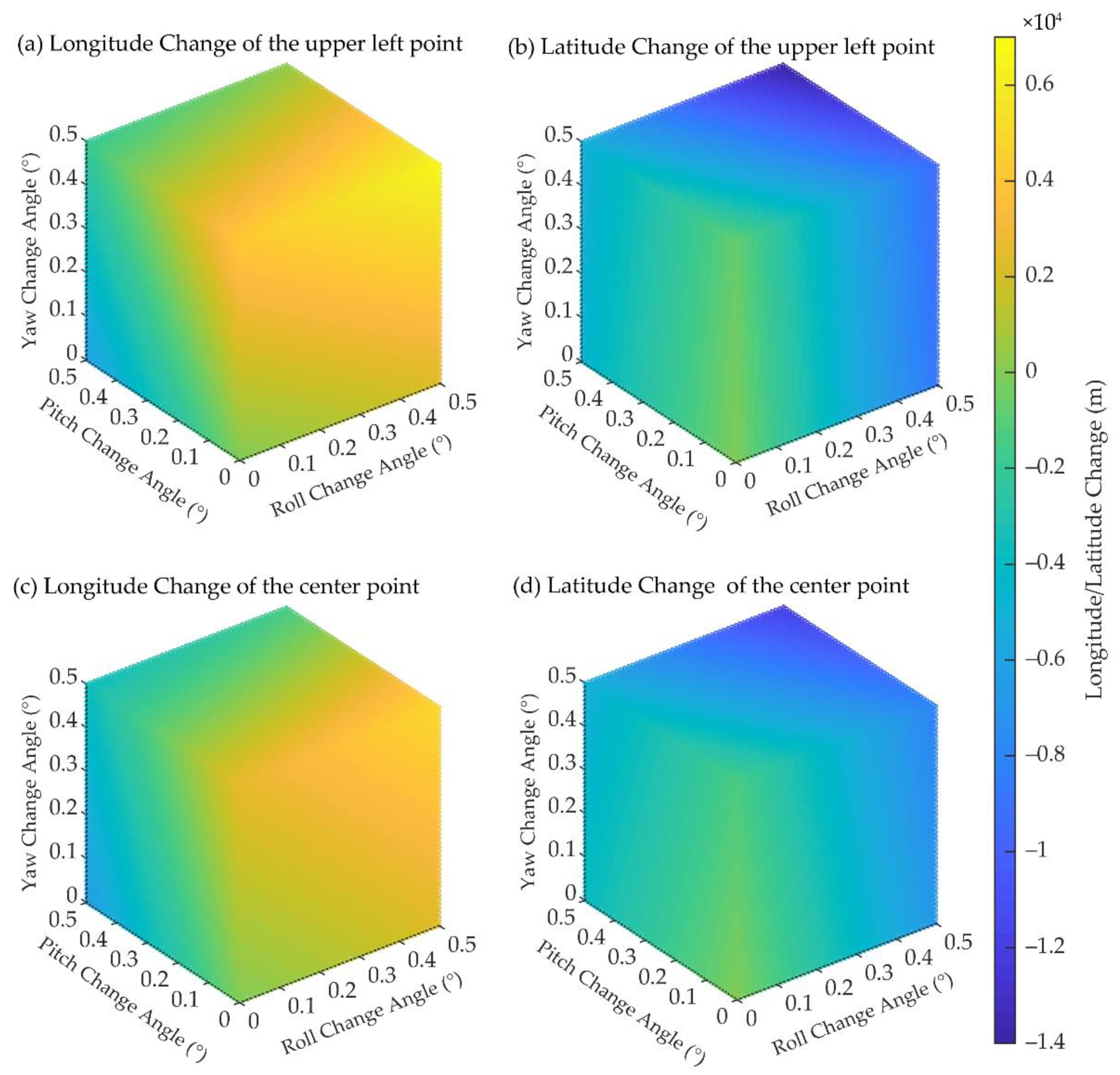
4.2. Uncertainty Evaluation of Geolocation of BNU-1 L1A Product
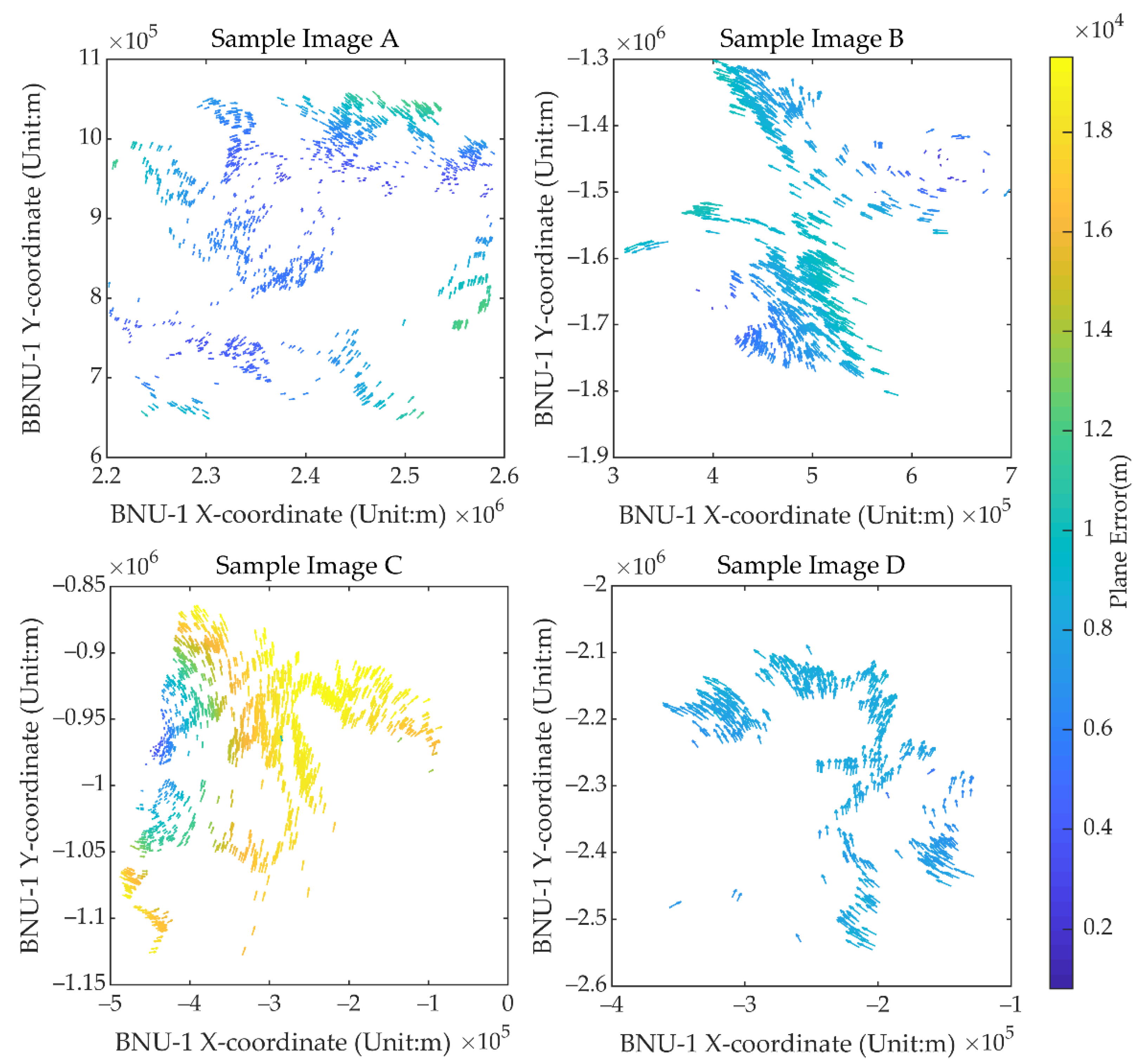
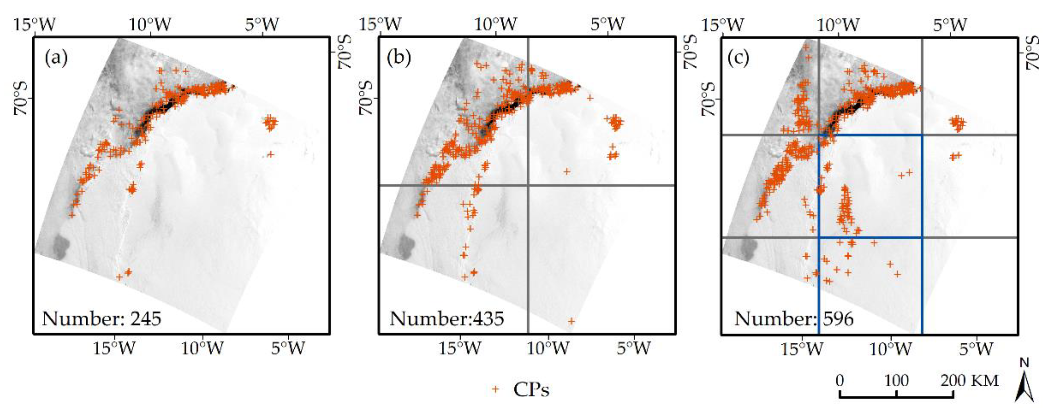
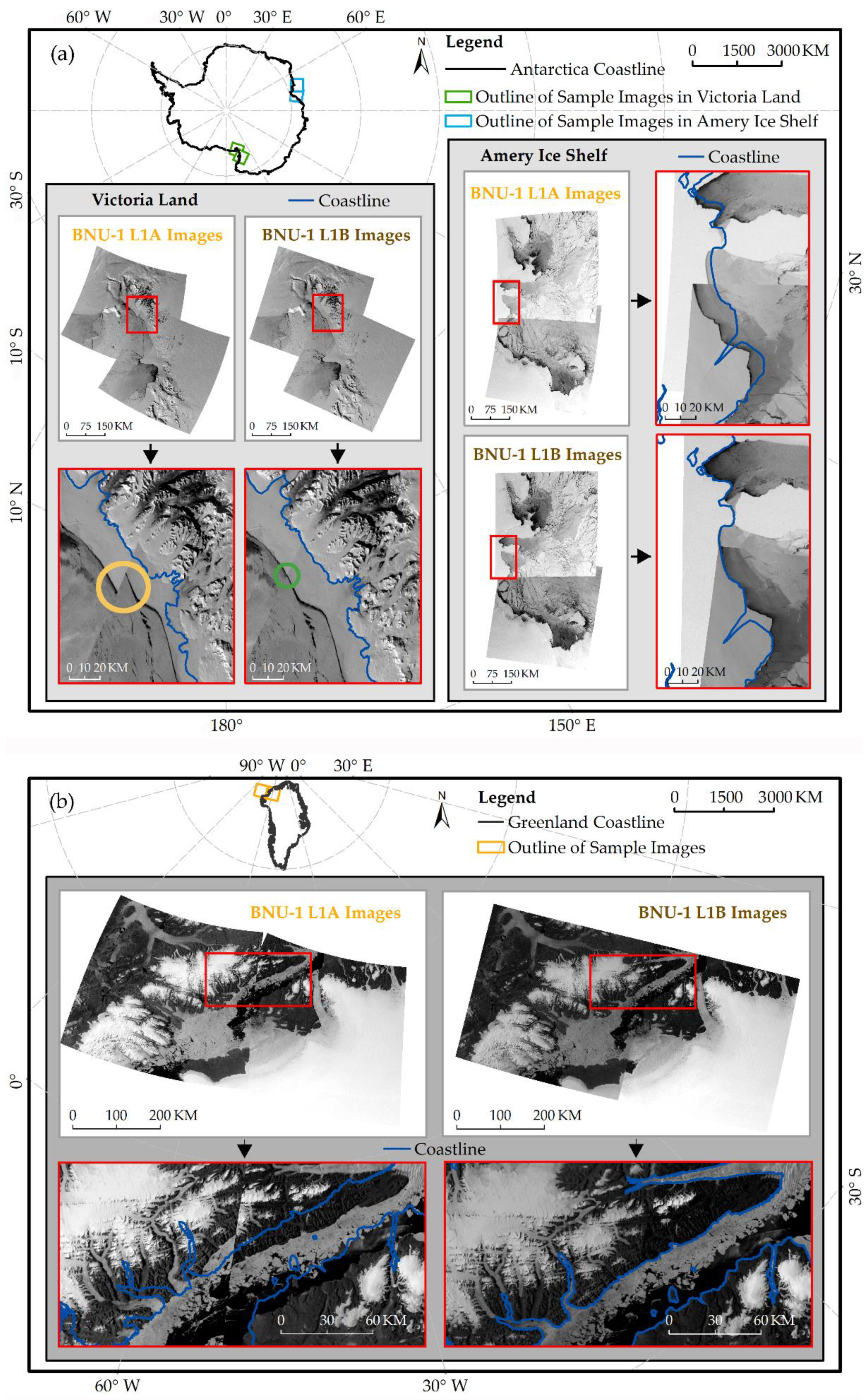
4.3. Influence of Image Division and Enhancement on the CPs Extraction
4.4. Geolocation Accuracy of the BNU-1 L1B Product
5. Discussion
6. Conclusions
Author Contributions
Funding
Institutional Review Board Statement
Informed Consent Statement
Data Availability Statement
Acknowledgments
Conflicts of Interest
References
- Chen, Z.; Chi, Z.; Zinglersen, K.B.; Tian, Y.; Wang, K.; Hui, F.; Cheng, X. A new image mosaic of greenland using Landsat-8 OLI images. Sci. Bull. 2020, 65, 522–524. [Google Scholar] [CrossRef] [Green Version]
- Ban, H.-J.; Kwon, Y.-J.; Shin, H.; Ryu, H.-S.; Hong, S. Flood monitoring using satellite-based RGB composite imagery and refractive index retrieval in visible and near-infrared bands. Remote Sens. 2017, 9, 313. [Google Scholar] [CrossRef] [Green Version]
- Schroeder, W.; Oliva, P.; Giglio, L.; Quayle, B.; Lorenz, E.; Morelli, F. Active fire detection using Landsat-8/OLI data. Remote Sens. Environ. 2016, 185, 210–220. [Google Scholar] [CrossRef] [Green Version]
- Gao, F.; Hilker, T.; Zhu, X.; Anderson, M.; Masek, J.; Wang, P.; Yang, Y. Fusing landsat and MODIS data for vegetation monitoring. IEEE Geosci. Remote Sens. Mag. 2015, 3, 47–60. [Google Scholar] [CrossRef]
- Miller, R.L.; McKee, B.A. Using MODIS Terra 250 m imagery to map concentrations of total suspended matter in coastal waters. Remote Sens. Environ. 2004, 93, 259–266. [Google Scholar] [CrossRef]
- Benn, D.I.; Cowton, T.; Todd, J.; Luckman, A. Glacier calving in greenland. Curr. Clim. Chang. Rep. 2017, 3, 282–290. [Google Scholar] [CrossRef] [Green Version]
- Yu, H.; Rignot, E.; Morlighem, M.; Seroussi, H. Iceberg calving of Thwaites Glacier, West Antarctica: Full-Stokes modeling combined with linear elastic fracture mechanics. Cryosphere 2017, 11, 1283–1296. [Google Scholar] [CrossRef] [Green Version]
- Liang, Q.I.; Zhou, C.; Howat, I.M.; Jeong, S.; Liu, R.; Chen, Y. Ice flow variations at Polar Record Glacier, East Antarctica. J. Glaciol. 2019, 65, 279–287. [Google Scholar] [CrossRef] [Green Version]
- Shen, Q.; Wang, H.; Shum, C.K.; Jiang, L.; Hsu, H.T.; Dong, J. Recent high-resolution Antarctic ice velocity maps reveal increased mass loss in Wilkes Land, East Antarctica. Sci Rep. 2018, 8, 4477. [Google Scholar] [CrossRef] [PubMed]
- Onarheim, I.H.; Eldevik, T.; Smedsrud, L.H.; Stroeve, J.C. Seasonal and regional manifestation of arctic sea ice loss. J. Clim. 2018, 31, 4917–4932. [Google Scholar] [CrossRef]
- Luo, Y.; Guan, K.; Peng, J.; Wang, S.; Huang, Y. STAIR 2.0: A generic and automatic algorithm to fuse modis, landsat, and Sentinel-2 to generate 10 m, daily, and cloud-/gap-free surface reflectance product. Remote Sens. 2020, 12, 3209. [Google Scholar] [CrossRef]
- Singh, L.A.; Whittecar, W.R.; DiPrinzio, M.D.; Herman, J.D.; Ferringer, M.P.; Reed, P.M. Low cost satellite constellations for nearly continuous global coverage. Nat. Commun. 2020, 11, 200. [Google Scholar] [CrossRef]
- Wolfe, R.E.; Nishihama, M.; Fleig, A.J.; Kuyper, J.A.; Roy, D.P.; Storey, J.C.; Patt, F.S. Achieving sub-pixel geolocation accuracy in support of MODIS land science. Remote Sens. Environ. 2002, 83, 31–49. [Google Scholar] [CrossRef]
- Moradi, I.; Meng, H.; Ferraro, R.R.; Bilanow, S. Correcting geolocation errors for microwave instruments aboard NOAA satellites. IEEE Trans. Geosci. Remote Sens. 2013, 51, 3625–3637. [Google Scholar] [CrossRef]
- Wang, M.; Cheng, Y.; Chang, X.; Jin, S.; Zhu, Y. On-orbit geometric calibration and geometric quality assessment for the high-resolution geostationary optical satellite GaoFen4. ISPRS-J. Photogramm. Remote Sens. 2017, 125, 63–77. [Google Scholar] [CrossRef]
- Toutin, T. Review article: Geometric processing of remote sensing images: Models, algorithms and methods. Int. J. Remote Sens. 2010, 25, 1893–1924. [Google Scholar] [CrossRef]
- Wang, J.; Ge, Y.; Heuvelink, G.B.M.; Zhou, C.; Brus, D. Effect of the sampling design of ground control points on the geometric correction of remotely sensed imagery. Int. J. Appl. Earth Obs. Geoinf. 2012, 18, 91–100. [Google Scholar] [CrossRef]
- Jiang, Y.; Zhang, G.; Wang, T.; Li, D.; Zhao, Y. In-orbit geometric calibration without accurate ground control data. Photogramm. Eng. Remote Sens. 2018, 84, 485–493. [Google Scholar] [CrossRef]
- Wang, X.; Li, Y.; Wei, H.; Liu, F. An ASIFT-based local registration method for satellite imagery. Remote Sens. 2015, 7, 7044–7061. [Google Scholar] [CrossRef] [Green Version]
- Feng, R.; Du, Q.; Shen, H.; Li, X. Region-by-region registration combining feature-based and optical flow methods for remote sensing images. Remote Sens. 2021, 13, 1475. [Google Scholar] [CrossRef]
- Goncalves, H.; Corte-Real, L.; Goncalves, J.A. Automatic image registration through image segmentation and SIFT. IEEE Trans. Geosci. Remote Sens. 2011, 49, 2589–2600. [Google Scholar] [CrossRef] [Green Version]
- Wang, L.; Niu, Z.; Wu, C.; Xie, R.; Huang, H. A robust multisource image automatic registration system based on the SIFT descriptor. Int. J. Remote Sens. 2011, 33, 3850–3869. [Google Scholar] [CrossRef]
- Khlopenkov, K.V.; Trishchenko, A.P. Implementation and evaluation of concurrent gradient search method for reprojection of MODIS level 1B imagery. IEEE Trans. Geosci. Remote Sens. 2008, 46, 2016–2027. [Google Scholar] [CrossRef]
- Xiong, X.; Che, N.; Barnes, W. Terra MODIS on-orbit spatial characterization and performance. IEEE Trans. Geosci. Remote Sens. 2005, 43, 355–365. [Google Scholar] [CrossRef]
- Gerrish, L.; Fretwell, P.; Cooper, P. High Resolution Vector Polylines of the Antarctic Coastline (7.4). 2021. Available online: 10.5285/e46be5bc-ef8e-4fd5-967b-92863fbe2835 (accessed on 20 October 2021).
- Haran, T.; Bohlander, J.; Scambos, T.; Painter, T.; Fahnestock, M. MEaSUREs MODIS Mosaic of Greenland (MOG) 2005, 2010, and 2015 Image Maps, Version 2. 2018. Available online: https://nsidc.org/data/nsidc-0547/versions/2 (accessed on 20 October 2021).
- Tang, X.; Zhang, G.; Zhu, X.; Pan, H.; Jiang, Y.; Zhou, P.; Wang, X. Triple linear-array image geometry model of ZiYuan-3 surveying satellite and its validation. Int. J. Image Data Fusion 2013, 4, 33–51. [Google Scholar] [CrossRef]
- Wang, M.; Yang, B.; Hu, F.; Zang, X. On-orbit geometric calibration model and its applications for high-resolution optical satellite imagery. Remote Sens. 2014, 6, 4391–4408. [Google Scholar] [CrossRef] [Green Version]
- Cao, J.; Yuan, X.; Gong, J.; Duan, M. The look-angle calibration method for on-orbit geometric calibration of ZY-3 satellite imaging sensors. Acta Geod. Cartogr. Sin. 2014, 43, 1039–1045. [Google Scholar]
- Guan, Z.; Jiang, Y.; Wang, J.; Zhang, G. Star-based calibration of the installation between the camera and star sensor of the Luojia 1-01 satellite. Remote Sens. 2019, 11, 2081. [Google Scholar] [CrossRef] [Green Version]
- Dave, C.P.; Joshi, R.; Srivastava, S.S. A survey on geometric correction of satellite imagery. Int. J. Comput. Appl. Technol. 2015, 116, 24–27. [Google Scholar]
- Zhang, G.; Xu, K.; Zhang, Q.; Li, D. Correction of pushbroom satellite imagery interior distortions independent of ground control points. Remote Sens. 2018, 10, 98. [Google Scholar] [CrossRef] [Green Version]
- Lowe, D.G. Distinctive image features from scale-invariant keypoints. Int. J. Comput. Vis. 2004, 60, 91–110. [Google Scholar] [CrossRef]
- Bindschadler, R.; Vornberger, P.; Fleming, A.; Fox, A.; Mullins, J.; Binnie, D.; Paulsen, S.; Granneman, B.; Gorodetzky, D. The landsat image mosaic of antarctica. Remote Sens. Environ. 2008, 112, 4214–4226. [Google Scholar] [CrossRef]
- Kouyama, T.; Kanemura, A.; Kato, S.; Imamoglu, N.; Fukuhara, T.; Nakamura, R. Satellite attitude determination and map projection based on robust image matching. Remote Sens. 2017, 9, 90. [Google Scholar] [CrossRef] [Green Version]
- Hu, C.M.; Tang, P. HJ-1A/B CCD IMAGERY Geometric distortions and precise geometric correction accuracy analysis. In Proceedings of the International Geoscience and Remote Sensing Symposium, Vancouver, BC, Canada, 24–29 July 2011; pp. 4050–4053. [Google Scholar]
- Li, Y.; He, L.; Ye, X.; Guo, D. Geometric correction algorithm of UAV remote sensing image for the emergency disaster. In Proceedings of the 2016 IEEE International Geoscience and Remote Sensing Symposium (IGARSS), Beijing, China, 10–15 July 2016; pp. 6691–6694. [Google Scholar]
- Wang, S.; Quan, D.; Liang, X.; Ning, M.; Guo, Y.; Jiao, L. A deep learning framework for remote sensing image registration. ISPRS-J. Photogramm. Remote Sens. 2018, 145, 148–164. [Google Scholar] [CrossRef]
- Ma, L.; Liu, Y.; Zhang, X.; Ye, Y.; Yin, G.; Johnson, B.A. Deep learning in remote sensing applications: A meta-analysis and review. ISPRS-J. Photogramm. Remote Sens. 2019, 152, 166–177. [Google Scholar] [CrossRef]


| Scene ID | RMSE | Scene ID | RMSE | ||
|---|---|---|---|---|---|
| L1A | L1B | L1A | L1B | ||
| Amery Ice Sheet | Victoria Land | ||||
| 1 (A) 1 | 6544.83 | 270.19 | 1 | 7639.83 | 412.85 |
| 2 | 8613.73 | 180.87 | 2 (B) | 7919.60 | 253.40 |
| 3 | 5061.16 | 234.17 | 3 | 4683.40 | 277.69 |
| 4 | 10,848.59 | 175.13 | 4 | 17,855.48 | 277.47 |
| 5 | 7079.49 | 245.66 | 5 | 8602.73 | 293.14 |
| 6 | 9572.81 | 237.79 | 6 | 17,380.35 | 339.21 |
| Dronning Maud Land | Greenland | ||||
| 1 | 5642.45 | 362.99 | 1 | 16,236.81 | 283.33 |
| 2 | 6916.70 | 243.97 | 2 | 19,828.19 | 189.23 |
| 3 | 3625.91 | 189.88 | 3 | 15,870.7 | 229.51 |
| 4 | 5680.75 | 203.38 | 4 | 12,435.58 | 299.84 |
| 5 | 6761.34 | 258.69 | 5 | 9959.07 | 321.84 |
| 6 | 8142.78 | 220.03 | 6 | 10,836.43 | 258.28 |
| 7 | 8012.31 | 324.15 | 7 | 7854.03 | 339.87 |
| 8 | 8036.76 | 484.89 | 8 | 18,738.91 | 178.34 |
| 9 | 7759.36 | 279.76 | 9 | 13,244.36 | 216.14 |
| 10 | 7007.99 | 203.37 | 10 (C) | 15,071.02 | 269.83 |
| 11 | 6786.16 | 242.65 | 11 | 13,489.89 | 265.7 |
| 12 | 5045.67 | 506.19 | 12 | 17,819.43 | 414.26 |
| 13 | 10,215.28 | 458.47 | 13 | 19,880.35 | 331.14 |
| 14 | 6880.00 | 575.88 | 14 | 16,219.35 | 292.06 |
| 15 (E) | 7309.43 | 221.59 | 15 (D) | 7778.63 | 302.29 |
| Pine Island Glacier | |||||
| 1(F) | 19,765.58 | 783.90 | |||
| Average | L1A: 10,480.31 L1B: 301.14 | ||||
| Sample Image | Number of CPs Extracted from the Original Image | Number of CPs Extracted from Scheme 1 | Number of CPs Extracted from Scheme 2 | Optimal Increment of CPs (%) 2 |
|---|---|---|---|---|
| A | 1071 | 2100 1 | 1840 | 96 |
| B | 935 | 2280 1 | 1624 | 144 |
| C | 1334 | 2236 1 | 1905 | 68 |
| D | 447 | 580 1 | 579 | 30 |
| E | 245 | 435 | 596 1 | 143 |
| F | 17 | 32 | 48 1 | 182 |
| Sample Image | Geolocation Accuracy of the Corrected BNU-1 Image (m) | Improvement in Geolocation Accuracy (%) | |
|---|---|---|---|
| Corrected by the CPs Extracted from the Original Image | Corrected by the CPs Extracted from the Optimal Scheme | ||
| A | 279.42 | 270.19 | 3.30 |
| B | 260.80 | 253.40 | 2.84 |
| C | 275.79 | 269.83 | 2.16 |
| D | 305.28 | 302.29 | 0.98 |
| E | 242.43 | 221.59 | 8.60 |
| F | /(Serious distortion) | 783.90 | / |
Publisher’s Note: MDPI stays neutral with regard to jurisdictional claims in published maps and institutional affiliations. |
© 2021 by the authors. Licensee MDPI, Basel, Switzerland. This article is an open access article distributed under the terms and conditions of the Creative Commons Attribution (CC BY) license (https://creativecommons.org/licenses/by/4.0/).
Share and Cite
Zhang, Y.; Chi, Z.; Hui, F.; Li, T.; Liu, X.; Zhang, B.; Cheng, X.; Chen, Z. Accuracy Evaluation on Geolocation of the Chinese First Polar Microsatellite (Ice Pathfinder) Imagery. Remote Sens. 2021, 13, 4278. https://doi.org/10.3390/rs13214278
Zhang Y, Chi Z, Hui F, Li T, Liu X, Zhang B, Cheng X, Chen Z. Accuracy Evaluation on Geolocation of the Chinese First Polar Microsatellite (Ice Pathfinder) Imagery. Remote Sensing. 2021; 13(21):4278. https://doi.org/10.3390/rs13214278
Chicago/Turabian StyleZhang, Ying, Zhaohui Chi, Fengming Hui, Teng Li, Xuying Liu, Baogang Zhang, Xiao Cheng, and Zhuoqi Chen. 2021. "Accuracy Evaluation on Geolocation of the Chinese First Polar Microsatellite (Ice Pathfinder) Imagery" Remote Sensing 13, no. 21: 4278. https://doi.org/10.3390/rs13214278