
Validation of Visually Interpreted Corine Land Cover Classes with Spectral Values of Satellite Images and Machine Learning

 , , , , , and
Abstract
:1. Introduction
2. Materials and Methods
2.1. Datasets
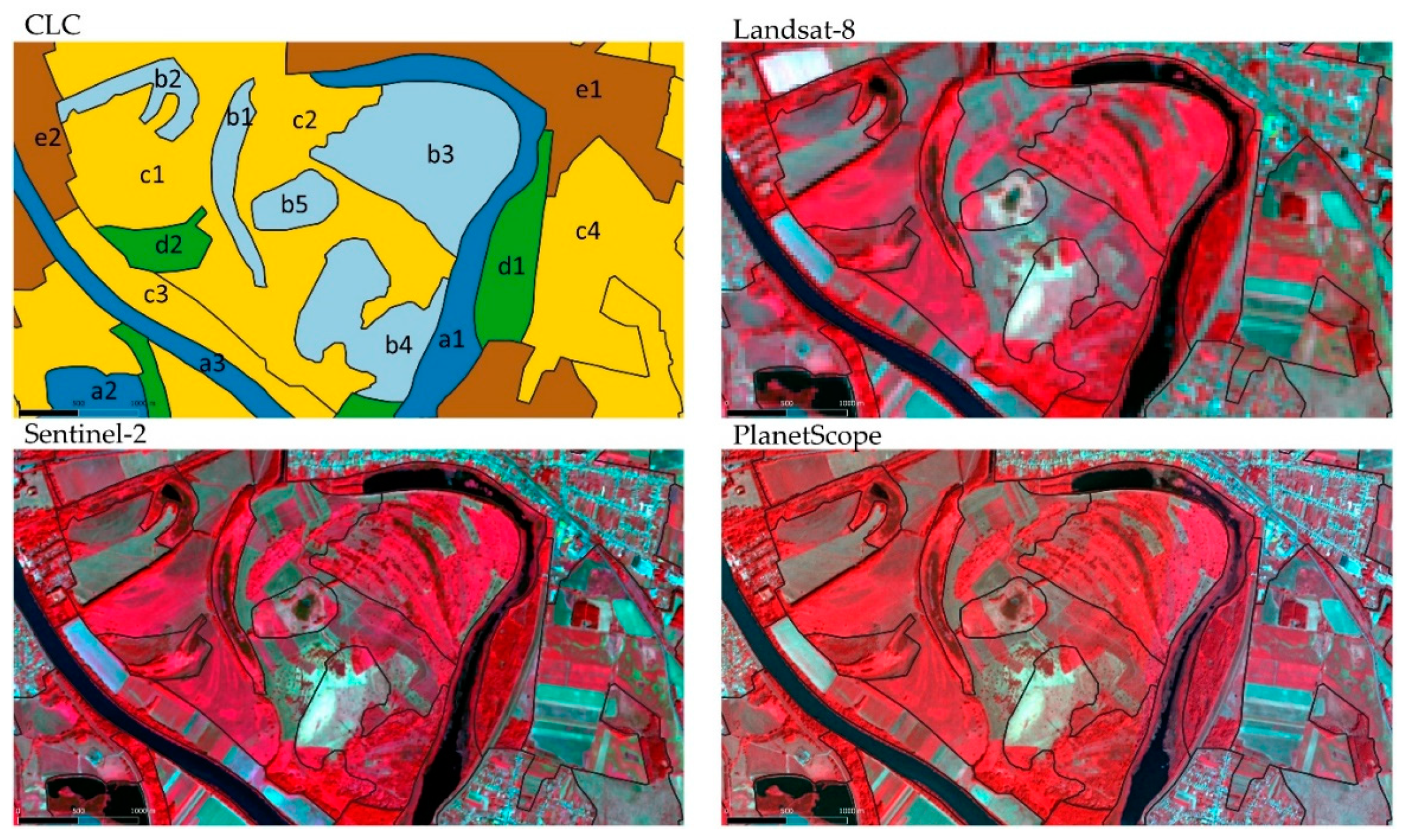
2.2. Study Area
2.3. Image Processing
2.4. Statistical Analysis
2.5. Analysis of Data Representativeness
2.6. Accuracy Assessment
3. Results
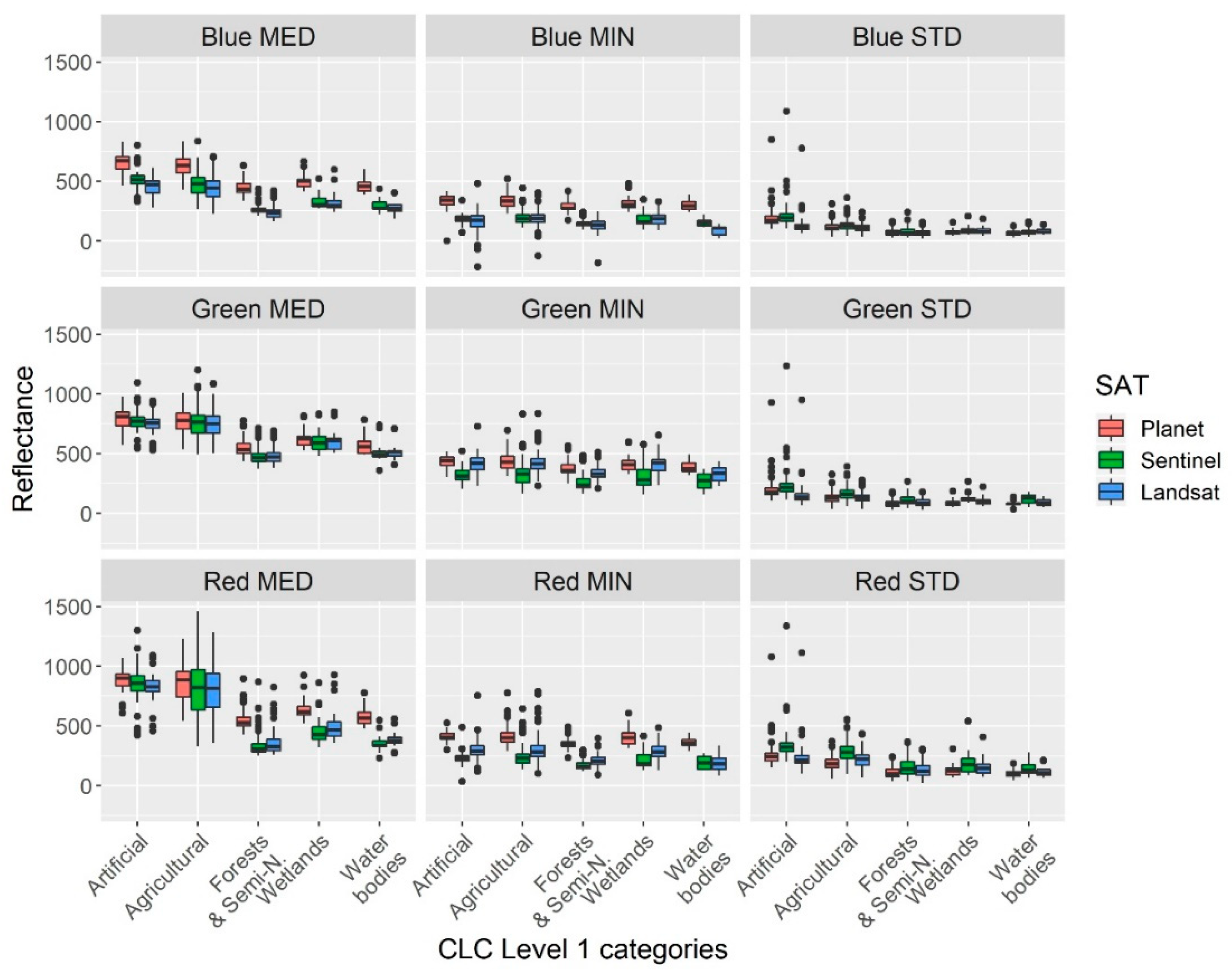
3.1. Differences of Spectral Characteristics of CLC Categories
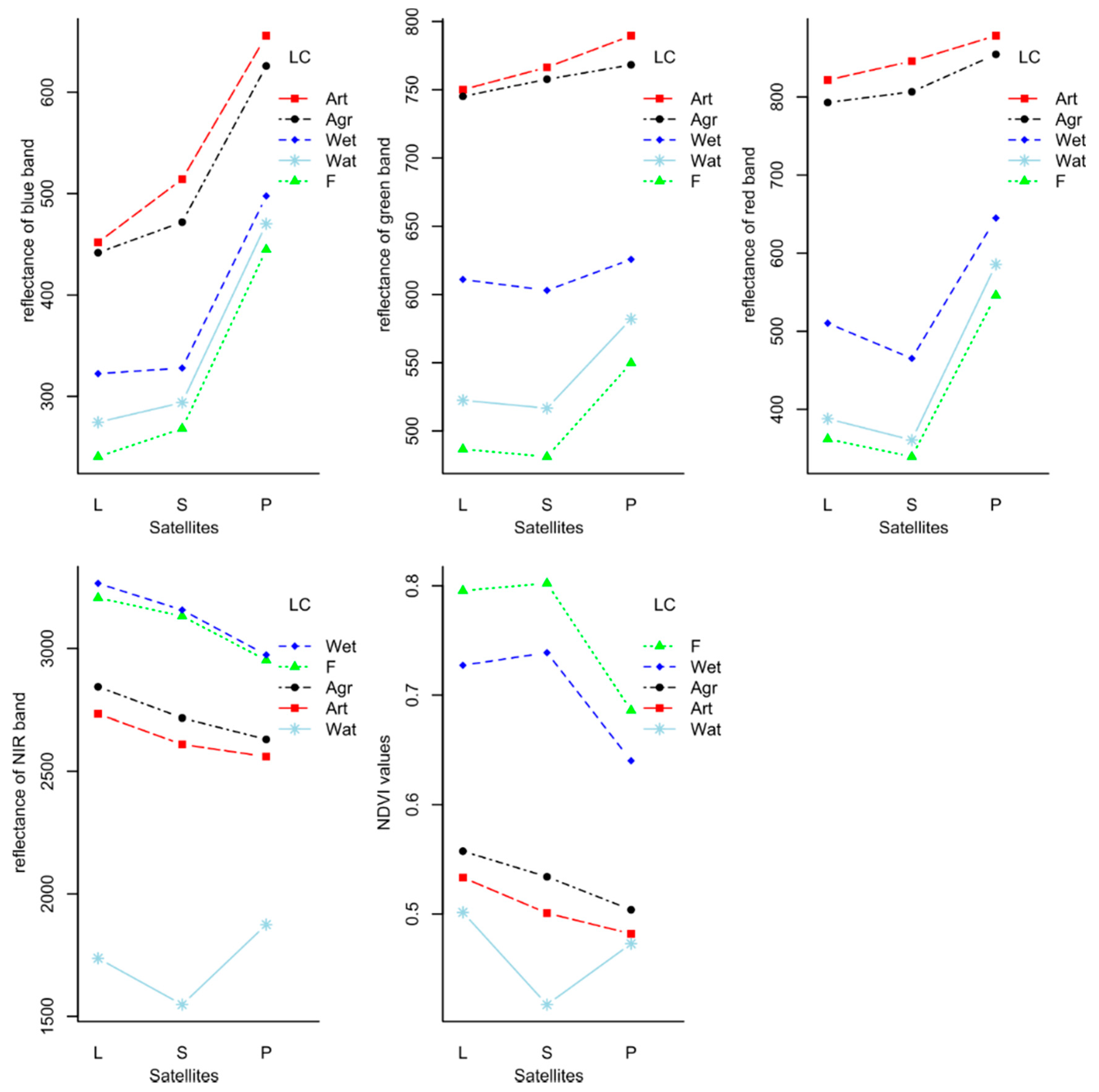
3.2. Reflectance Values and Nominal Factors
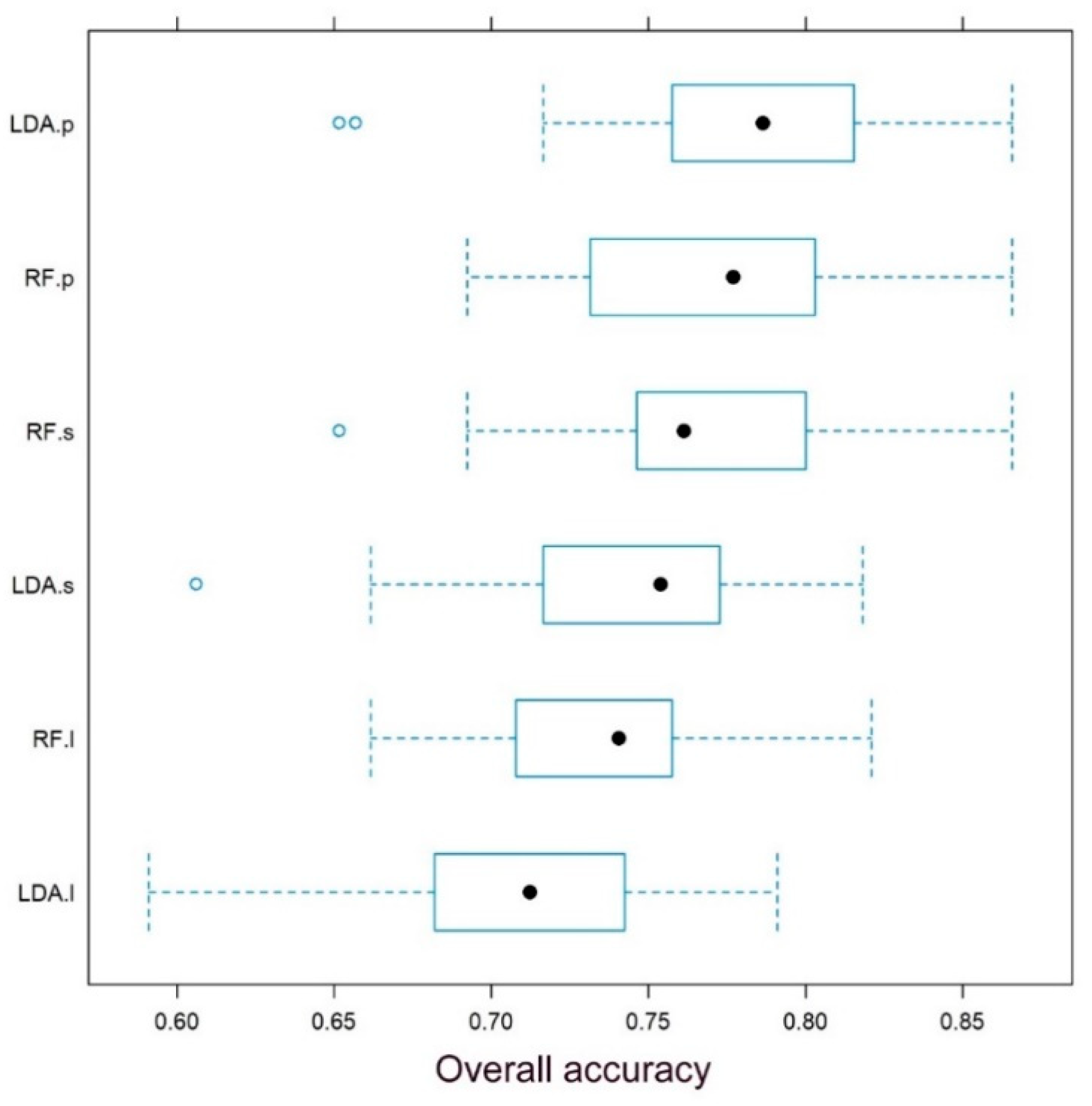
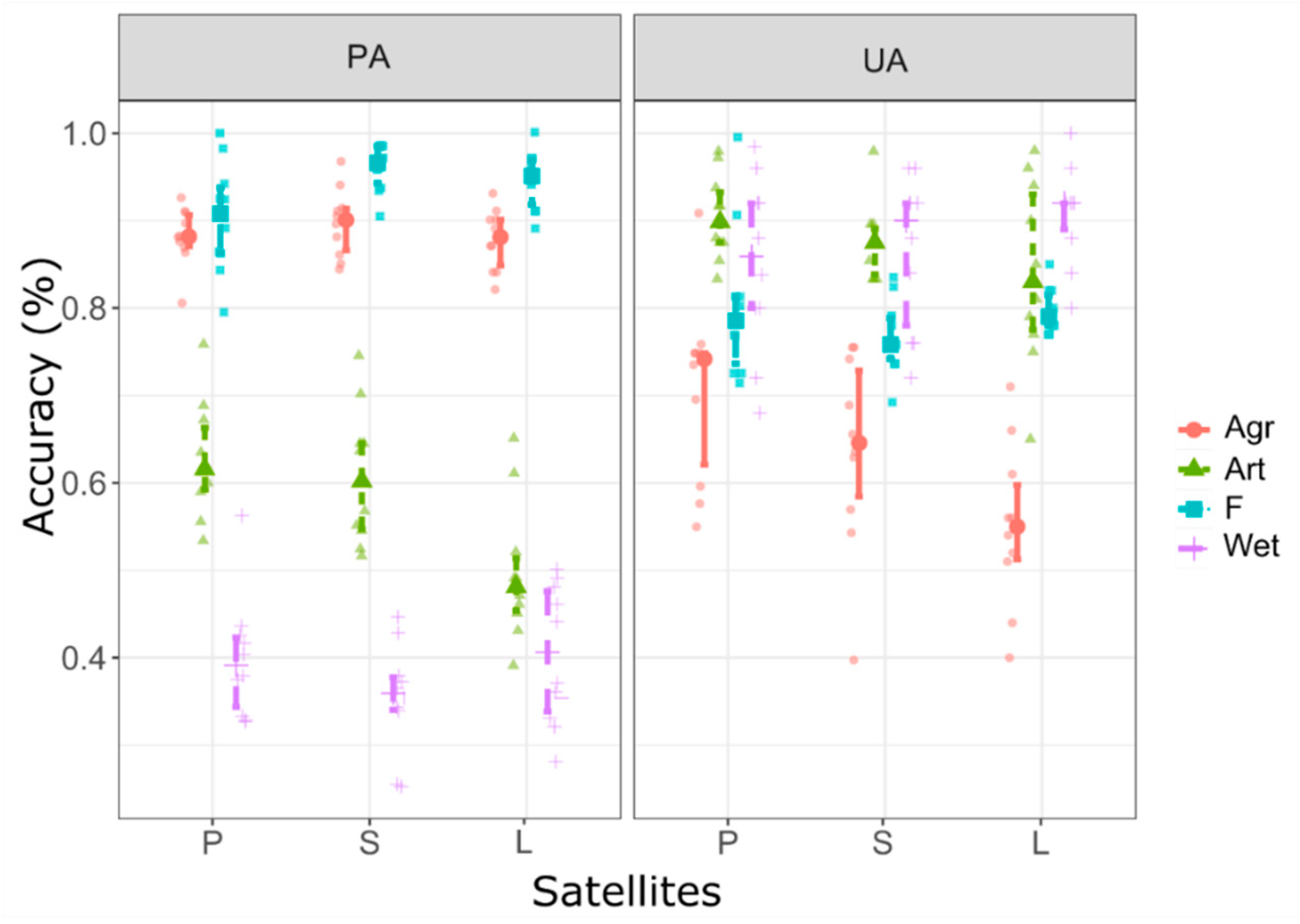
3.3. CLC Categories as Reflected in Classification Algorithms
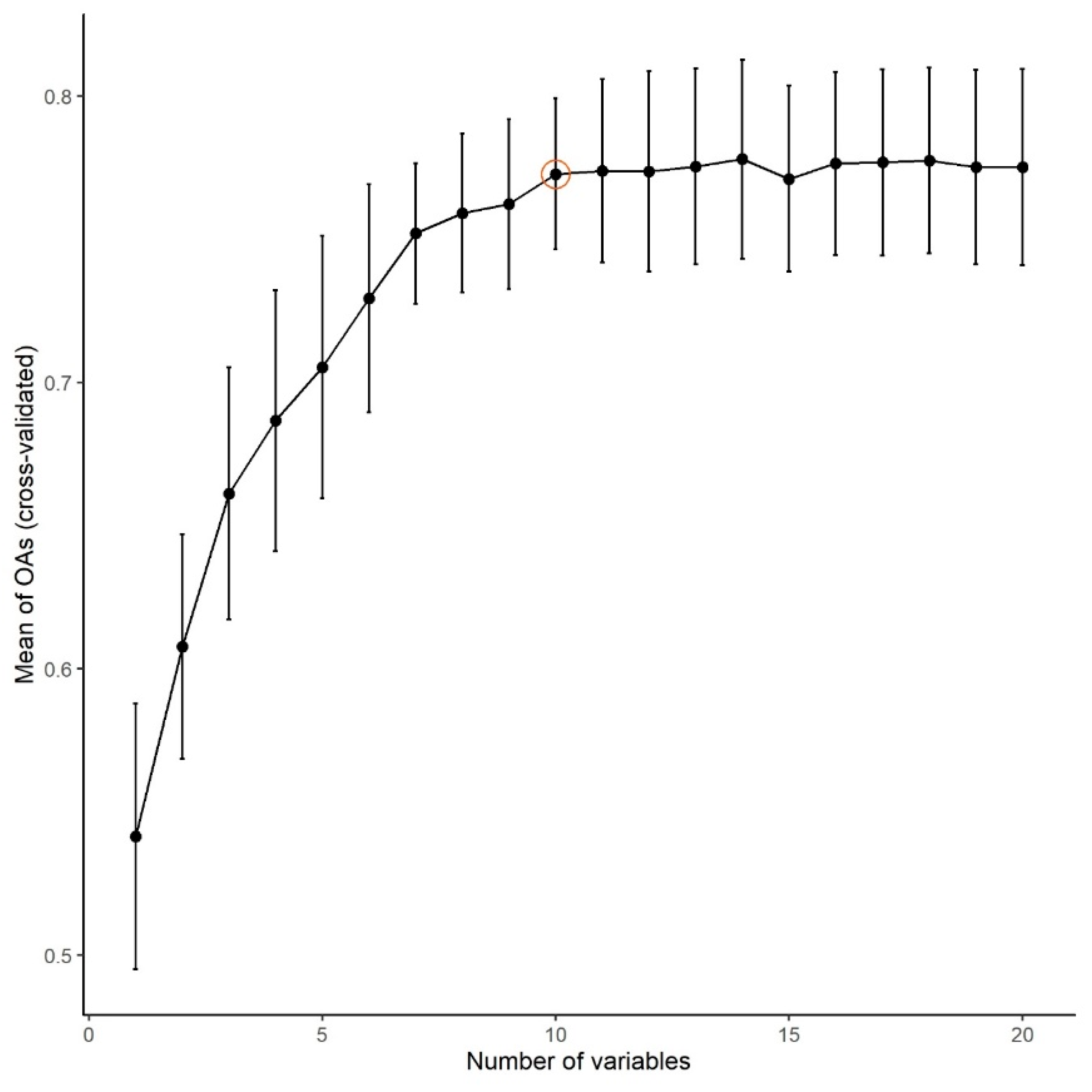
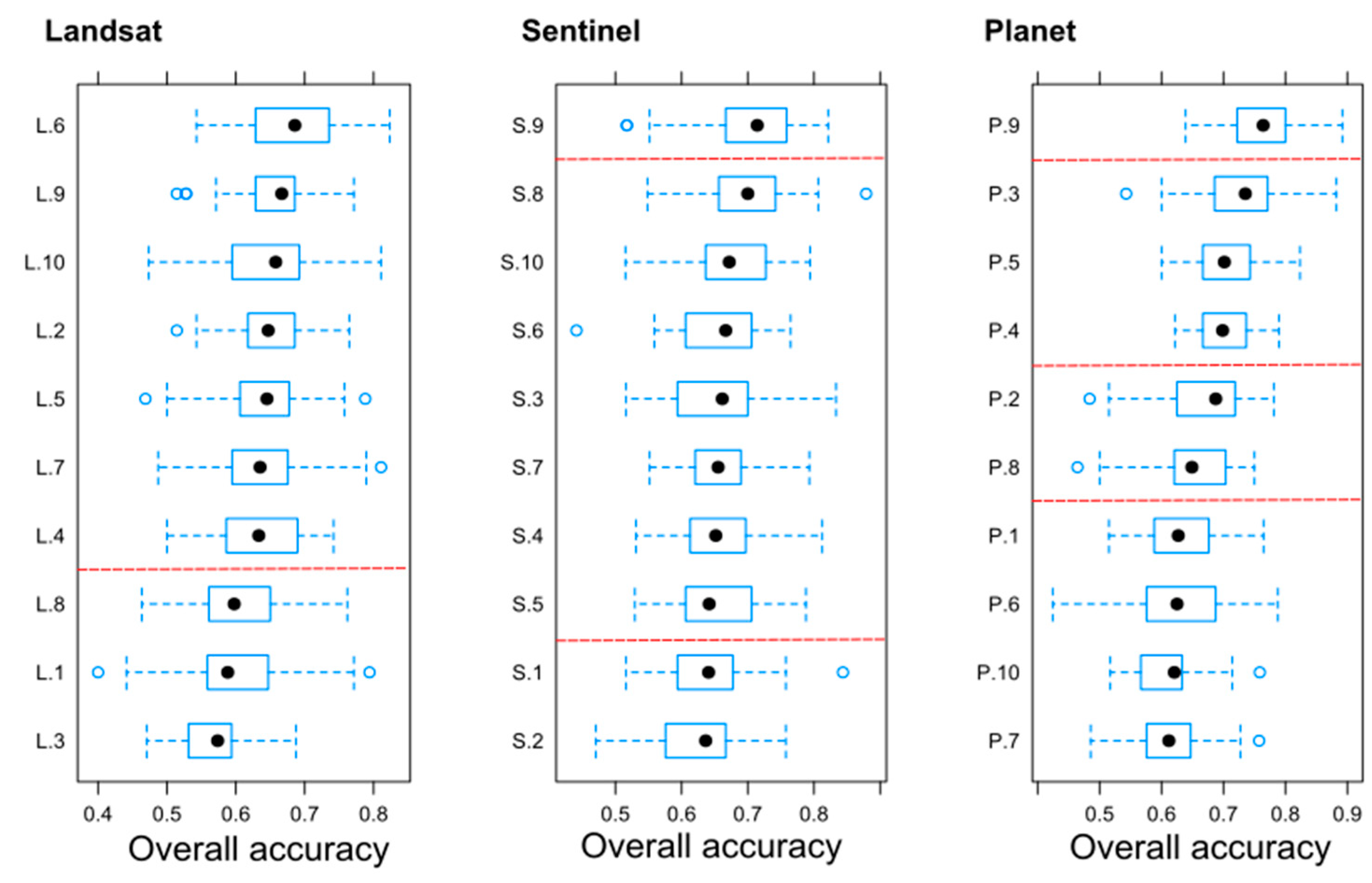
3.4. Data Representativeness
4. Discussion
4.1. CLC Classes and the Mixture of Spectral Features
4.2. CLC Classes in the Light of Statistical Tests
4.3. CLC Classes and Classification Algorithms
5. Conclusions
- -
- Medians of CLC polygons provided the least mixture among the LC classes, while the maximums were the worst input parameters without significant differences. Wetlands and water bodies categories were the most frequently mixing categories of CLC based on reflectance values;
- -
- Bivariate statistical tests cannot provide enough information to conclude on the spectral separability of LC classes, but classification algorithms involving several variables can be efficient techniques. Generally, LDA and RF classifiers had similar OAs, but in the case of coarser resolutions (Sentinel and Landsat), RF outperformed the LDA. Data derived from PlanetScope provided 7% better OAs (78%) than those of Landsat (71%) regarding the model medians; thus, better spatial resolution ensured better classification performance. >80% OA was gained with using all available bands of the Sentinel-2; accordingly, more spectral information in the infra-red range can counterbalance the coarser geometric resolution;
- -
- We applied a randomization-based technique to gain 10 repetitions of class-level metrics (UA and PA), which showed that satellites had no direct effect on the accuracy. UAs were the lowest in agricultural areas, while PAs were the lowest among wetlands;
- -
- Variable importance of statistical parameters showed that usually the medians were the most important statistical layers, and the green, red and near-infrared bands were the first three most important bands;
- -
- We provided an approach to prove the possibility of the generalization of the results with multiple randomized subsampling and found that the results of Landsat and Sentinel data can be generalized, but in the case of PlanetScope, a larger area with more CLC polygons would be desirable;
- -
- Generally, using the overlapping bands (RGB + NIR) of Landsat-8, Sentinel-2 with the PlanetScope, the best OAs were >70% OAs, but the most accurate was the PlanetScope with the highest spatial resolution (78.5%). Higher OAs (~80%) have also been acquired with the higher spectral accuracy of the Sentinel-2, which means a cost-efficient solution in spite of the coarser spatial resolution;
- -
- As we found several studies where CLC maps were used as ground truth data to quantify thematic accuracy, 70–80% OAs do not seem satisfactory. Nevertheless, our experiment was performed with the CLC L1 classes; further investigations can reveal if CLC is more appropriate for ground truth with the more detailed L2 or L3 nomenclature.
Author Contributions
Funding
Data Availability Statement
Conflicts of Interest
References
- Deák, M.; Telbisz, T.; Árvai, M.; Mari, L.; Horváth, F.; Kohán, B. Heterogeneous Forest Classification by Creating Mixed Vegetation Classes using EO-1 Hyperion. Int. J. Remote Sens. 2017, 38, 5215–5231. [Google Scholar] [CrossRef] [Green Version]
- Kishor, B.; Singh, S.K. Change Detection Mapping of Land use Land Cover using Multidate Satellite Data (A Case Study of Pichavaram Mangrove). Int. J. Eng. Res. Technol. 2014, 3, 2320–2326. [Google Scholar]
- Sohl, T.L.; Sleeter, B.M. Role of Remote Sensing for Land-Use and Land- Cover Change Modelling. In Remote Sensing and Land Cover: Principles and Applications; Giri, C., Ed.; CRC Press: Boca Raton, FL, USA, 2012; pp. 225–239. [Google Scholar]
- Bey, A.; Sánchez-Paus Díaz, A.; Maniatis, D.; Marchi, G.; Mollicone, D.; Ricci, S.; Bastin, J.; Moore, R.; Federici, S.; Rezende, M.; et al. Collect Earth: Land use and Land Cover Assessment through Augmented Visual Interpretation. Remote Sens. 2016, 8, 807. [Google Scholar] [CrossRef] [Green Version]
- Burai, P.; Deák, B.; Valkó, O.; Tomor, T. Classification of Herbaceous Vegetation using Airborne Hyperspectral Imagery. Remote Sens. 2015, 7, 2046–2066. [Google Scholar] [CrossRef] [Green Version]
- Li, X.; Chen, W.; Cheng, X.; Wang, L. A Comparison of Machine Learning Algorithms for Mapping of Complex Surface-Mined and Agricultural Landscapes using ZiYuan-3 Stereo Satellite Imagery. Remote Sens. 2016, 8, 514. [Google Scholar] [CrossRef] [Green Version]
- Wessel, M.; Brandmeier, M.; Tiede, D. Evaluation of Different Machine Learning Algorithms for Scalable Classification of Tree Types and Tree Species Based on Sentinel-2 Data. Remote Sens. 2018, 10, 1419. [Google Scholar] [CrossRef] [Green Version]
- Abd El-Kawy, O.R.; Rød, J.K.; Ismail, H.A.; Suliman, A.S. Land use and Land Cover Change Detection in the Western Nile Delta of Egypt using Remote Sensing Data. Appl. Geogr. 2011, 31, 483–494. [Google Scholar] [CrossRef]
- Almeida, C.A.; Coutinho, A.C.; Esquerdo, J.C.D.M.; Adami, M.; Venturieri, A.; Diniz, C.G.; Dessay, N.; Durieux, L.G.; Rodrigues, A. High Spatial Resolution Land use and Land Cover Mapping of the Brazilian Legal Amazon in 2008 using Landsat-5/TM and MODIS Data. Acta Amaz. 2016, 46, 291–302. [Google Scholar] [CrossRef]
- Pinto, A.T.; Gonçalves, J.A.; Beja, P.; Pradinho Honrado, J. From Archived Historical Aerial Imagery to Informative Orthophotos: A Framework for Retrieving the Past in Long-Term Socioecological Research. Remote Sens. 2019, 11, 1388. [Google Scholar] [CrossRef] [Green Version]
- Bielecka, E.; Jenerowicz, A. Intellectual Structure of CORINE Land Cover Research Applications in Web of Science: A Europe-Wide Review. Remote Sens. 2019, 11, 2017. [Google Scholar] [CrossRef] [Green Version]
- Chehdi, K.; Cariou, C. Learning or Assessment of Classification Algorithms Relying on Biased Ground Truth Data: What Interest? J. Appl. Remote Sens. 2019, 13, 034522. [Google Scholar] [CrossRef]
- Congalton, R.G. A Review of Assessing the Accuracy of Classifications of Remotely Sensed Data. Remote Sens. Environ. 1991, 37, 35–46. [Google Scholar] [CrossRef]
- Hay, A.H. Sampling Designs to Test Land-use Map Accuracy. Photogramm. Eng. Remote Sens. 1979, 45, 529–533. [Google Scholar]
- Yague, J.; Garcia, P. Approaching Corine Land Cover Over Castilla and Leon (Central Spain) with a Multitemporal NOAA-AVHRR NDVI MVC Series. In Proceedings of the Second International Workshop on the Analysis of Multi-Temporal Remote Sensing Images; Smits, P.C., Bruzzone, L., Eds.; World Scientific Publishing: Singapore, 2004; pp. 314–321. [Google Scholar]
- De Santa Olalla Mañas, M.; Soria, C.; Ramírez, A. Validation of the CORINE Land Cover Database in a Pilot Zone Under Semi-Arid Conditions in La Mancha (Spain). Cybergeo Eur. J. Geogr. 2003. [Google Scholar] [CrossRef]
- Rujoiu-Mare, M.; Mihai, B. Mapping Land Cover using Remote Sensing Data and GIS Techniques: A Case Study of Prahova Subcarpathians. Procedia Environ. Sci. 2016, 32, 244–255. [Google Scholar] [CrossRef] [Green Version]
- Caetano, M.; Mata, F.; Freire, S. Accuracy assessment of the Portuguese CORINE Land Cover map. In Global Developments in Environmental Earth Observation from Space; Marçal, A., Ed.; Millpress: Rotterdam, The Netherlands, 2006. [Google Scholar]
- Gudmann, A.; Csikós, N.; Szilassi, P.; Mucsi, L. Improvement in Satellite Image-Based Land Cover Classification with Landscape Metrics. Remote Sens. 2020, 12, 3580. [Google Scholar] [CrossRef]
- Stathopoulou, M.I.; Cartalis, C.; Petrakis, M. Integrating Corine Land Cover Data and Landsat TM for Surface Emissivity Definition: Application to the Urban Area of Athens, Greece. Int. J. Remote Sens. 2007, 28, 3291–3304. [Google Scholar] [CrossRef]
- Golenia, M.; Zagajewski, B.; Ochytra, A. Semiautomatic Land Cover Mapping According to the 2nd Level of the CORINE Land Cover Legend. Pol. Cartogr. Rev. 2015, 47, 203–212. [Google Scholar] [CrossRef] [Green Version]
- Dalponte, M.; Marzini, S.; Solano-Correa, Y.T.; Tonon, G.; Vescovo, L.; Gianelle, D. Mapping Forest Windthrows using High Spatial Resolution Multispectral Satellite Images. Int. J. Appl. Earth Obs. Geoinf. 2020, 93, 102206. [Google Scholar] [CrossRef]
- Messina, G.; Peña, J.M.; Vizzari, M.; Modica, G. A Comparison of UAV and Satellites Multispectral Imagery in Monitoring Onion Crop an Application in the ‘Cipolla Rossa Di Tropea’ (Italy). Remote Sens. 2020, 12, 3424. [Google Scholar] [CrossRef]
- Feranec, J.; Soukup, T.; Hazeu, G.; Jaffrain, G. European Landscape Dynamics: CORINE Land Cover Data; CRC Press: Boca Raton, FL, USA, 2016. [Google Scholar]
- Leinenkugel, P.; Deck, R.; Huth, J.; Ottinger, M.; Mack, B. The Potential of Open Geodata for Automated Large-Scale Land use and Land Cover Classification. Remote Sens. 2019, 11, 2249. [Google Scholar] [CrossRef] [Green Version]
- European Environment Agency (EEA). Corine Land Cover Change (CHA) 2012–2018; Version 2020_20u1; European Environment Agency: Copenhagen, Denmark, 2020; Available online: https://land.copernicus.eu/pan-european/corine-land-cover/lcc-2012-2018?tab=download (accessed on 24 February 2021).
- Kosztra, B.; Büttner, G.; Hazeu, G.; Arnold, S. Updated CLC Illustrated Nomenclature Guidelines. European Topic Centre on Urban, Land and Soil Systems. 2019. Available online: https://land.copernicus.eu/user-corner/technical-library/corine-land-cover-nomenclature-guidelines/docs/pdf/CLC2018_Nomenclature_illustrated_guide_20190510.pdf (accessed on 24 February 2021).
- U.S. Geological Survey. Landsat 8 Fact Sheet 2013-3060. 2013. Available online: https://pubs.usgs.gov/fs/2013/3060/pdf/fs2013-3060.pdf (accessed on 24 February 2021).
- European Space Agency. Sentinel-2 User Handbook. 2015. Available online: https://sentinel.esa.int/documents/247904/685211/Sentinel-2_User_Handbook (accessed on 24 February 2021).
- Planet Labs. Planet Imagery Product Specifications. 2019. Available online: https://assets.planet.com/docs/Planet_Combined_Imagery_Product_Specs_letter_screen.pdf (accessed on 24 February 2021).
- The Hungarian Meteorological Service (OMSZ). Daily Weather Forecast for Hungary 2005–2019. Available online: https://www.met.hu/idojaras/aktualis_idojaras/napijelentes_2005-2019/ (accessed on 24 February 2021).
- Rouse, J.W., Jr.; Haas, R.H.; Schell, J.A.; Deering, D.W.; Harlan, J.C. Monitoring the Vernal Advancements and Retrogradation of Natural Vegetation; Final Report; NASA Goddard Space Flight Center: Greenbelt, MD, USA, 1974; pp. 1–137. [Google Scholar]
- Baret, F.; Guyot, G.; Major, D.J. Crop Biomass Evaluation using Radiometric Measurements. Photogrammetria 1989, 43, 241–256. [Google Scholar] [CrossRef]
- Aredehey, G.; Mezgebu, A.; Girma, A. Land-use Land-Cover Classification Analysis of Giba Catchment using Hyper Temporal MODIS NDVI Satellite Images. Int. J. Remote Sens. 2018, 39, 810–821. [Google Scholar] [CrossRef]
- Gulácsi, A.; Kovács, F. Drought Monitoring of Forest Vegetation using MODIS-Based Normalized Difference Drought Index in Hungary. Hung. Geogr. Bull. 2018, 67, 29–42. [Google Scholar] [CrossRef] [Green Version]
- Szabó, S.; Elemér, L.; Kovács, Z.; Püspöki, Z.; Kertész, Á.; Singh, S.K.; Balázs, B. NDVI Dynamics as Reflected in Climatic Variables: Spatial and Temporal Trends—A Case Study of Hungary. GISci. Remote Sens. 2019, 56, 624–644. [Google Scholar] [CrossRef]
- Ma, J.; Zhang, C.; Yun, W.; Lv, Y.; Wanling, C.; Zu, D. The Temporal Analysis of Regional Cultivated Land Productivity with GPP Based on 2000–2018 MODIS Data. Sustainability 2020, 12, 411. [Google Scholar] [CrossRef] [Green Version]
- Olmos-Trujillo, E.; González-Trinidad, J.; Júnez-Ferreira, H.; Pacheco-Guerrero, A.; Bautista-Capetillo, C.; Avila-Sandoval, C.; Galván-Tejada, E. Spatio-Temporal Response of Vegetation Indices to Rainfall and Temperature in A Semiarid Region. Sustainability 2020, 12, 1939. [Google Scholar] [CrossRef] [Green Version]
- Roy, D.P.; Yan, L. Robust Landsat-Based Crop Time Series Modelling. Remote Sens. Environ. 2020, 238, 110810. [Google Scholar] [CrossRef]
- Dövényi, Z. Inventory of Microregions in Hungary; MTA Földrajztudományi Kutatóintézet: Budapest, Hungary, 2010. [Google Scholar]
- QGIS Development Team. QGIS Geographic Information System. Open Source Geospatial Foundation Project 2020. Available online: http://qgis.osgeo.org (accessed on 23 February 2021).
- R Core Team. R: A Language and Environment for Statistical Computing; R Foundation for Statistical Computing: Vienna, Austria, 2020. [Google Scholar]
- Wickham, H. Ggplot2: Elegant Graphics for Data Analysis; Springer: New York, NY, USA, 2016. [Google Scholar]
- Hothorn, T.; Bretz, F.; Westfall, P. Simultaneous Inference in General Parametric Models. Biom. J. 2008, 50, 346–363. [Google Scholar] [CrossRef] [Green Version]
- Field, A. Discovering Statistics Using IBM SPSS Statistics, 4th ed.; SAGE Publications Ltd.: Thousand Oaks, CA, USA, 2013. [Google Scholar]
- Albers, C.; Lakens, D. When Power Analyses Based on Pilot Data are Biased: Inaccurate Effect Size Estimators and Follow-Up Bias. J. Exp. Soc. Psychol. 2018, 74, 187–195. [Google Scholar] [CrossRef] [Green Version]
- The Jamovi Project—Jamovi Version 1.2.16. 2020. Available online: https://www.jamovi.org (accessed on 23 February 2021).
- Abriha, D.; Kovács, Z.; Ninsawat, S.; Bertalan, L.; Boglárka, B.; Szabó, S. Identification of Roofing Materials with Discriminant Function Analysis and Random Forest Classifiers on Pan-Sharpened WorldView-2 Imagery—A Comparison. Hung. Geogr. Bull. 2018, 67, 375–392. [Google Scholar] [CrossRef] [Green Version]
- Feldesman, M.R. Classification Trees as an Alternative to Linear Discriminant Analysis. Phys. Anthropol. 2002, 119, 257–275. [Google Scholar] [CrossRef]
- Rekabdar, G.; Soleymani, B. Effect of Sampling Methods on Misclassification of Fisher’s Linear Discriminant Analysis. Int. J. Stat. Appl. 2015, 5, 208–212. [Google Scholar]
- Phinzi, K.; Abriha, D.; Bertalan, L.; Holb, I.; Szabó, S. Machine Learning for Gully Feature Extraction Based on a Pan-Sharpened Multispectral Image: Multiclass Vs. Binary Approach. Int. J. Geo-Inf. 2020, 9, 252. [Google Scholar] [CrossRef] [Green Version]
- Archibald, R.; Fann, G. Feature Selection and Classification of Hyperspectral Images with Support Vector Machines. IEEE Geosci. Remote. Sens. Lett. 2007, 4, 674–677. [Google Scholar] [CrossRef]
- Kuhn, M. Caret: Classification and Regression Training. R Package Version 6.0-85. 2020. Available online: https://cran.r-project.org/web/packages/caret/caret.pdf (accessed on 23 February 2021).
- Foody, G.M. Sample Size Determination for Image Classification Accuracy Assessment and Comparison. Int. J. Remote Sens. 2009, 30, 5273–5291. [Google Scholar] [CrossRef]
- Chen, Q.; Meng, Z.; Liu, X.; Jin, Q.; Su, R. Decision Variants for the Automatic Determination of Optimal Feature Subset in RF-RFE. Genes 2018, 9, 301. [Google Scholar] [CrossRef] [Green Version]
- Büttner, G.; Kosztra, B. CLC2018 Technical Guidelines; European Environmental Agency: Wien, Austria, 2017; p. 61. Available online: https://land.copernicus.eu/user-corner/technical-library/clc2018technicalguidelines_final.pdf (accessed on 24 February 2021).
- European Environment Agency. The Thematic Accuracy of Corine Land Cover 2000, Assessment using LUCAS (Land use/Cover Area Frame Statistical Survey); EEA Technical report No 7/2006; European Environmental Agency: Copenhangen, Denmark, 2006. [Google Scholar]
- Petropoulos, G.P.; Kalaitzidis, C.; Prasad Vadrevu, K. Support Vector Machines and Object-Based Classification for Obtaining Land-use/Cover Cartography from Hyperion Hyperspectral Imagery. Comput. Geosci. 2012, 41, 99–107. [Google Scholar] [CrossRef]
- Tormos, T.; Dupuy, S.; van Looy, K.; Barbe, E.; Kosuth, P. An OBIA for Fine-Scale Land Cover Spatial Analysis Over Broad Territories: Demonstration through Riparian Corridor and Artificial Sprawl Studies in France. In Proceedings of the 4th International Conference on Geographic Object-Based Image Analysis (GEOBIA), Rio de Janeiro, Brazil, 7–9 May 2012. [Google Scholar]
- Forman, R.T.T.; Godron, M. Landscape Ecology; John Wiley & Sons: New York, NY, USA, 1986. [Google Scholar]
- Reyes, A.; Solla, M.; Lorenzo, H. Comparison of Different Object-Based Classifications in LandsatTM Images for the Analysis of Heterogeneous Landscapes. Measurement 2017, 97, 29–37. [Google Scholar] [CrossRef]
- Ceccarelli, T.; Smiraglia, D.; Bajocco, S.; Rinaldo, S.; De Angelis, A.; Salvati, L.; Perini, L. Land Cover Data from Landsat Single-Date Imagery: An Approach Integrating Pixel-Based and Objectbased Classifiers. Eur. J. Remote Sens. 2013, 46, 699–717. [Google Scholar] [CrossRef]
- Verde, N.; Kokkoris, I.P.; Georgiadis, C.; Kaimaris, D.; Dimopoulos, P.; Mitsopoulos, I.; Mallinis, G. National Scale Land Cover Classification for Ecosystem Services Mapping and Assessment, using Multitemporal Copernicus EO Data and Google Earth Engine. Remote Sens. 2020, 12, 3303. [Google Scholar] [CrossRef]
- Blaschke, T. Object Based Image Analysis for Remote Sensing. ISPRS J. Photogramm. Remote Sens. 2010, 65, 2–16. [Google Scholar] [CrossRef] [Green Version]
- Sannier, C.; Jaffrain, G.; Bossard, M.; Feranec, J.; Pennec, A.; Di Federico, A. Corine Land Cover 2012 Final Validation Report. 2017. Available online: https://land.copernicus.eu/user-corner/technical-library/clc-2012-validation-report-1 (accessed on 24 February 2021).
- Burai, P.; Lövei, G.Z.; Lénárt, C.; Nagy, I.; Enyedi, P. Mapping Aquatic Vegetation of the Rakamaz-Tiszanagyfalui Nagy-Morotva using Hyperspectral Imagery. Landsc. Environ. 2010, 4, 1–10. [Google Scholar]
- Szabó, Z.; Tóth, C.A.; Tomor, T.; Szabó, S. Airborne LiDAR Point Cloud in Mapping of Fluvial Forms: A Case Study of a Hungarian Floodplain. GIScience Remote Sens. 2017, 54, 862–880. [Google Scholar] [CrossRef]
- Szabó, Z.; Tóth, C.A.; Holb, I.; Szabó, S. Aerial Laser Scanning Data as a Source of Terrain Modelling in a Fluvial Environment: Biasing Factors of Terrain Height Accuracy. Sensors 2020, 20, 2063. [Google Scholar] [CrossRef] [PubMed] [Green Version]
- Szabó, Z.; Buró, B.; Szabó, J.; Tóth, C.A.; Baranyai, E.; Herman, P.; Prokisch, J.; Tomor, T.; Szabó, S. Geomorphology as a Driver of Heavy Metal Accumulation Patterns in a Floodplain. Water 2020, 12, 563. [Google Scholar] [CrossRef] [Green Version]
- Härmä, P.; Autio, I.; Teiniranta, R.; Hatunen, S.; Törmä, M.; Kallio, M.; Kaartinen, M. Final Report. Copernicus Land Monitoring 2014–2020 in the Framework of Regulation (EU) No 377/2014 of the European Parliament and of the Council of 3 April 2014. Available online: https://www.google.com/url?sa=t&rct=j&q=&esrc=s&source=web&cd=&ved=2ahUKEwi1we6sgf3uAhVD8hQKHensAUkQFjAAegQIARAD&url=https%3A%2F%2Fwww.syke.fi%2Fdownload%2Fnoname%2F%257B725215CE-EE17-4B5F-A531-CD525425B28C%257D%2F144830&usg=AOvVaw3mzg_A8PEwDsm0tuZONzdv (accessed on 24 February 2021).
- Jeevalakshmi, D.; Narayana Reddy, S.; Manikiam, B. Land Cover Classification Based on NDVI using LANDSAT8 Time Series: A Case Study Tirupati Region. In Proceedings of the 2016 International Conference on Communication and Signal Processing (ICCSP), Melmaruvathur, India, 6–8 April 2016. [Google Scholar]
- Pu, R.; Gong, P.; Tian, Y.; Miao, X.; Carruthers, R.I.; Anderson, G.L. Using Classification and NDVI Differencing Methods for Monitoring Sparse Vegetation Coverage: A Case Study of Saltcedar in Nevada, USA. Int. J. Remote Sens. 2008, 29, 3987–4011. [Google Scholar] [CrossRef]
- Taufik, A.; Ahmad, S.S.S.; Ahmad, A. Classification of Landsat 8 Satellite Data using NDVI Thresholds. J. Telecommun. Electron. Comput. Eng. 2016, 8, 37–40. [Google Scholar]
- Zhang, X.; Wu, S.; Yan, X.; Chen, Z. A Global Classification of Vegetation Based on NDVI, Rainfall and Temperature. Int. J. Climatol. 2017, 37, 2318–2324. [Google Scholar] [CrossRef]
- Miomir, J.M.; Milanović, M.M.; Vračarević, B.R. Comparing NDVI and Corine Land Cover as Tools for Improving National Forest Inventory Updates and Preventing Illegal Logging in Serbia. In Vegetation; Sebata, A., Ed.; IntechOpen: London, UK, 2017. [Google Scholar]
- Diaz-Pacheco, J.; Gutiérrez, J. Exploring the Limitations of CORINE Land Cover for Monitoring Urban Landuse Dynamics in Metropolitan Areas. J. Land Use Sci. 2014, 9, 243–259. [Google Scholar] [CrossRef]
- Martínez-Fernández, J.; Ruiz-Benito, P.; Bonet, A.; Gómez, C. Methodological Variations in the Production of CORINE Land Cover and Consequences for Long-Term Land Cover Change Studies. The Case of Spain. Int. J. Remote Sens. 2019, 40, 8914–8932. [Google Scholar] [CrossRef] [Green Version]
- Rosina, K.; Batista e Silva, F.; Vizcaino, P.; Herrera, M.M.; Freire, S. Increasing the Detail of European Land use/Cover Data by Combining Heterogeneous Data Sets. Int. J. Digital Earth 2018, 13, 602–626. [Google Scholar] [CrossRef]
- Lekaj, E.; Teqja, Z. Investigation of Green Space Changes in Tirana-Durres Region. In Proceedings of the Third International Conference in Challenges in Biotechnological and Environmental Approaches, Tirana, Albania, 23–25 April 2019. [Google Scholar]
- Belgiu, M.; Drăguţ, L. Random Forest in Remote Sensing: A Review of Applications and Future Directions. ISPRS J. Photogramm. Remote Sens. 2016, 114, 24–31. [Google Scholar] [CrossRef]
- Millard, K.; Richardson, M. On the Importance of Training Data Sample Selection in Random Forest Image Classification: A Case Study in Peatland Ecosystem Mapping. Remote Sens. 2015, 7, 8489–8515. [Google Scholar] [CrossRef] [Green Version]
- Szabó, L.; Burai, P.; Deák, B.; Dyke, G.J.; Szabó, S. Assessing the Efficiency of Multispectral Satellite and Airborne Hyperspectral Images for Land Cover Mapping in an Aquatic Environment with Emphasis on the Water Caltrop (Trapa Natans). Int. J. Remote Sens. 2019, 40, 5192–5215. [Google Scholar] [CrossRef]
- Underwood, E.C.; Ustin, S.L.; Ramirez, C.M. A Comparison of Spatial and Spectral Image Resolution for Mapping Invasive Plants in Coastal California. Environ. Manag. 2007, 39, 63–83. [Google Scholar] [CrossRef]
- Balázs, B.; Bíró, T.; Dyke, G.; Singh, S.K.; Szabó, S. Extracting Water-Related Features using Reflectance Data and Principal Component Analysis of Landsat Images. Hydrol. Sci. J. 2018, 63, 269–284. [Google Scholar] [CrossRef]
- Kaplan, G.; Avdan, U. Object-Based Water Body Extraction Model using Sentinel-2 Satellite Imagery. Eur. J. Remote Sens. 2017, 50, 137–143. [Google Scholar] [CrossRef] [Green Version]
- Van Leeuwen, B.; Tobak, Z.; Kovács, F. Sentinel-1 and -2 Based Near Real Time Inland Excess Water Mapping for Optimized Water Management. Sustainability 2020, 12, 2854. [Google Scholar] [CrossRef] [Green Version]
- Chen, D.; Stow, D.A.; Gong, P. Examining the Effect of Spatial Resolution and Texture Window Size on Classification Accuracy: An Urban Environment Case. Int. J. Remote Sens. 2004, 25, 2177–2192. [Google Scholar] [CrossRef]
- Pu, R.; Landry, S.; Yu, Q. Object-Based Urban Detailed Land Cover Classification with High Spatial Resolution IKONOS Imagery. Int. J. Remote Sens. 2011, 32, 3285–3308. [Google Scholar] [CrossRef] [Green Version]
- Chiang, S.; Valdez, M. Tree Species Classification by Integrating Satellite Imagery and Topographic Variables using Maximum Entropy Method in a Mongolian Forest. Forests 2019, 10, 961. [Google Scholar] [CrossRef] [Green Version]
- Puletti, N.; Chianucci, F.; Castaldi, C. Use of Sentinel-2 for Forest Classification in Mediterranean Environments. Ann. Silvic. Res. 2018, 42, 32–38. [Google Scholar]
- Grabska, E.; Hostert, P.; Pflugmacher, D.; Ostapowicz, K. Forest Stand Species Mapping using the Sentinel-2 Time Series. Remote Sens. 2019, 11, 1197. [Google Scholar] [CrossRef] [Green Version]
- Amrhein, V.; Korner-Nievergelt, F.; Roth, T. The Earth is Flat (P > 0.05): Significance Thresholds and the Crisis of Unreplicable Research. PeerJ 2017, 5, 3544. [Google Scholar] [CrossRef] [Green Version]
- Urdan, T.C. Statistics in Plain English, 4th ed.; Taylor & Francis/Routledge: New York, NY, USA, 2016. [Google Scholar]
- Carrasco, L.; O’Neil, A.W.R.; Daniel, M.; Rowland, C.S. Evaluating Combinations of Temporally Aggregated Sentinel-1, Sentinel-2 and Landsat 8 for Land Cover Mapping with Google Earth Engine. Remote Sens. 2019, 11, 288. [Google Scholar] [CrossRef] [Green Version]
- Gong, X.; Shen, L.; Lu, T. Refining Training Samples using Median Absolute Deviation for Supervised Classification of Remote Sensing Images. J. Indian Soc. Remote Sens. 2019, 47, 647–659. [Google Scholar] [CrossRef]


| Mean Square | F Value | p (Significance) | |||||||
|---|---|---|---|---|---|---|---|---|---|
| SAT | L1 | SAT:L1 | SAT | L1 | SAT:L1 | SAT | L1 | SAT:L1 | |
| Blue | 3,486,511 | 2,126,014 | 6485 | 566.633 | 345.523 | 1.054 | <0.001 | <0.001 | 0.393 |
| Green | 132,930 | 3,269,793 | 14,691 | 14.815 | 364.426 | 1.637 | <0.001 | <0.001 | 0.11 |
| Red | 1,235,635 | 8,846,234 | 136,225 | 53.362 | 382.032 | 5.883 | <0.001 | <0.001 | <0.001 |
| NIR | 3,659,005 | 20,970,015 | 228,477 | 34.800 | 199.442 | 2.173 | <0.001 | <0.001 | 0.027 |
| NDVI | 0.4460 | 3.0034 | 0.0451 | 41.224 | 277.630 | 4.166 | <0.001 | <0.001 | <0.001 |
| SS | df | F | p | ω2 | |
|---|---|---|---|---|---|
| Model | 4.84 × 10⁹ | 74 | 2281.66 | <0.001 | 0.972 |
| Band | 2.07 × 10⁹ | 4 | 18,055.72 | <0.001 | 0.416 |
| SAT | 1.55 × 10⁶ | 2 | 27.01 | <0.001 | 0.000 |
| L1 | 2.80 × 10⁷ | 4 | 243.67 | <0.001 | 0.006 |
| Band × SAT | 6.24 × 10⁶ | 8 | 27.19 | <0.001 | 0.001 |
| Band × L1 | 1.13 × 10⁸ | 16 | 245.97 | <0.001 | 0.023 |
| SAT × L1 | 718,073 | 8 | 3.13 | 0.002 | 0.000 |
| Band × SAT × L1 | 2.37 × 10⁶ | 32 | 2.58 | <0.001 | 0.000 |
| Residuals | 1.39 × 10⁸ | 4845 | |||
| Total | 4.98 × 10⁹ | 4919 |
| SS | df | F | p | ω2 | |
|---|---|---|---|---|---|
| Model | 2.64 × 10⁸ | 75 | 562.59 | <0.001 | 0.895 |
| Band | 1.52 × 10⁸ | 5 | 4850.22 | <0.001 | 0.515 |
| SAT | 1.44 × 10⁶ | 2 | 115.10 | <0.001 | 0.005 |
| L1 | 2.77 × 10⁶ | 4 | 110.65 | <0.001 | 0.009 |
| Band × SAT | 1.43 × 10⁶ | 8 | 28.58 | <0.001 | 0.005 |
| Band × L1 | 1.12 × 10⁷ | 16 | 111.86 | <0.001 | 0.038 |
| SAT × L1 | 325,839 | 8 | 6.52 | <0.001 | 0.001 |
| Band × SAT × L1 | 411,950 | 32 | 2.06 | <0.001 | 0.001 |
| Residuals | 3.03 × 10⁷ | 4845 | |||
| Total | 2.94 × 10⁸ | 4920 |
| Models | Min | LQ | Median | Mean | UQ | Max |
|---|---|---|---|---|---|---|
| 4-band input (RGB + NIR) | ||||||
| LDA.l | 0.59 | 0.68 | 0.71 | 0.71 | 0.74 | 0.79 |
| RF.l | 0.66 | 0.71 | 0.74 | 0.74 | 0.76 | 0.82 |
| LDA.s | 0.61 | 0.72 | 0.75 | 0.75 | 0.77 | 0.82 |
| RF.s | 0.65 | 0.75 | 0.76 | 0.77 | 0.80 | 0.87 |
| All available bands | ||||||
| LDA.l | 0.66 | 0.71 | 0.74 | 0.75 | 0.79 | 0.88 |
| RF.l | 0.66 | 0.72 | 0.76 | 0.75 | 0.79 | 0.88 |
| LDA.s | 0.67 | 0.78 | 0.81 | 0.81 | 0.83 | 0.91 |
| RF.s | 0.68 | 0.75 | 0.78 | 0.78 | 0.80 | 0.88 |
Publisher’s Note: MDPI stays neutral with regard to jurisdictional claims in published maps and institutional affiliations. |
© 2021 by the authors. Licensee MDPI, Basel, Switzerland. This article is an open access article distributed under the terms and conditions of the Creative Commons Attribution (CC BY) license (http://creativecommons.org/licenses/by/4.0/).
Share and Cite
Varga, O.G.; Kovács, Z.; Bekő, L.; Burai, P.; Csatáriné Szabó, Z.; Holb, I.; Ninsawat, S.; Szabó, S. Validation of Visually Interpreted Corine Land Cover Classes with Spectral Values of Satellite Images and Machine Learning. Remote Sens. 2021, 13, 857. https://doi.org/10.3390/rs13050857
Varga OG, Kovács Z, Bekő L, Burai P, Csatáriné Szabó Z, Holb I, Ninsawat S, Szabó S. Validation of Visually Interpreted Corine Land Cover Classes with Spectral Values of Satellite Images and Machine Learning. Remote Sensing. 2021; 13(5):857. https://doi.org/10.3390/rs13050857
Chicago/Turabian StyleVarga, Orsolya Gyöngyi, Zoltán Kovács, László Bekő, Péter Burai, Zsuzsanna Csatáriné Szabó, Imre Holb, Sarawut Ninsawat, and Szilárd Szabó. 2021. "Validation of Visually Interpreted Corine Land Cover Classes with Spectral Values of Satellite Images and Machine Learning" Remote Sensing 13, no. 5: 857. https://doi.org/10.3390/rs13050857