Analysis of the Double-Bounce Interaction between a Random Volume and an Underlying Ground, Using a Controlled High-Resolution PolTomoSAR Experiment

Abstract

The radar response of vegetated environments, and forested areas in particular, are usually modeled using a very simple structure made of a random volume, representing a cloud of vegetation particles, lying over a semi-infinite medium with a rough interface, associated with the underlying ground. This Random Volume over Ground model can efficiently handle double-bounce scattering mechanisms, or arbitrary volume reflectivity profiles. This paper proposes to analyze a specific component of the Random Volume over Ground simplified scattering model, which concerns the double-bounce interaction between the ground and the volume. This specific contribution is not considered by classical characterization techniques and is studied in this work using a controlled experiment involving a Synthetic Aperture Radar operated in a Polarimetric and Tomographic configuration in order to image in 3D a controlled miniaturized scene composed of volume lying over a ground. It is shown that ground/volume double-bounce scattering, which remains focused at the ground level even in 3D imaging mode, and has polarimetric patterns that differ largely from those usually expected from double-bounce reflections, with volume-like features, such as a strong cross-polarized reflectivity or decorrelation between co-polarized channels. Moreover, it is shown that the full rank polarimetric patterns of the ground-volume mechanism are tightly linked to the reflectivity of the volume and may mask the ground response. As a consequence, isolating the ground response using 3D imaging does not permit to avoid a generally very strong distortion of the soil response by the double-bounce reflection, and the estimation of different geophysical parameters of the ground, such as its humidity or roughness are significantly altered.

1. Introduction

This paper focuses on the characterization of the Ground/Volume (GV) Double-Bounce (DB) scattering mechanism occurring during the measurement of a volumetric scattering medium lying over the ground. Volume imaging using Polarimetric SAR Tomography (PolTomSAR) has been widely applied to the study of natural environments like forests [1,2,3,4,5,6,7,8,9,10,11,12,13,14,15]. Such scenes consist of a ground surface and a vegetated medium that is composed of trunks and randomly oriented particles considered as a volume. Nevertheless, even if it may be used to improve the description of complex volumetric scenes, 3D imaging may still be affected by ambiguous behaviors, related to a finite resolution of analysis or to high-order scattering terms. Most of the studies [1,2,3,6,7,8,9,10,13,15] conducted in order to characterize vegetated 3D environments concentrated on the analysis of the observed volume. Only a few of them [4,5,11,12,14] addressed the underlying ground response too. In order to discriminate and assess the different mechanisms that participate in the interaction between an emitted radar wave and a forested area, a man-made miniaturized Random Volume over Ground (RVoG)-like scene is imaged using PolTomSAR in high-resolution, based on the transmission and reception of electromagnetic (EM) waves. The objects in the scene can be hidden, removed, or replaced, while the control of ground roughness and humidity, and volume length, height, and position may be used to test a series of hypotheses on the different physical phenomena occurring during a measurement. This setup will, hence, allow for highlighting the presence and locations of occurring scattering mechanisms, as well as to study their polarimetric features.

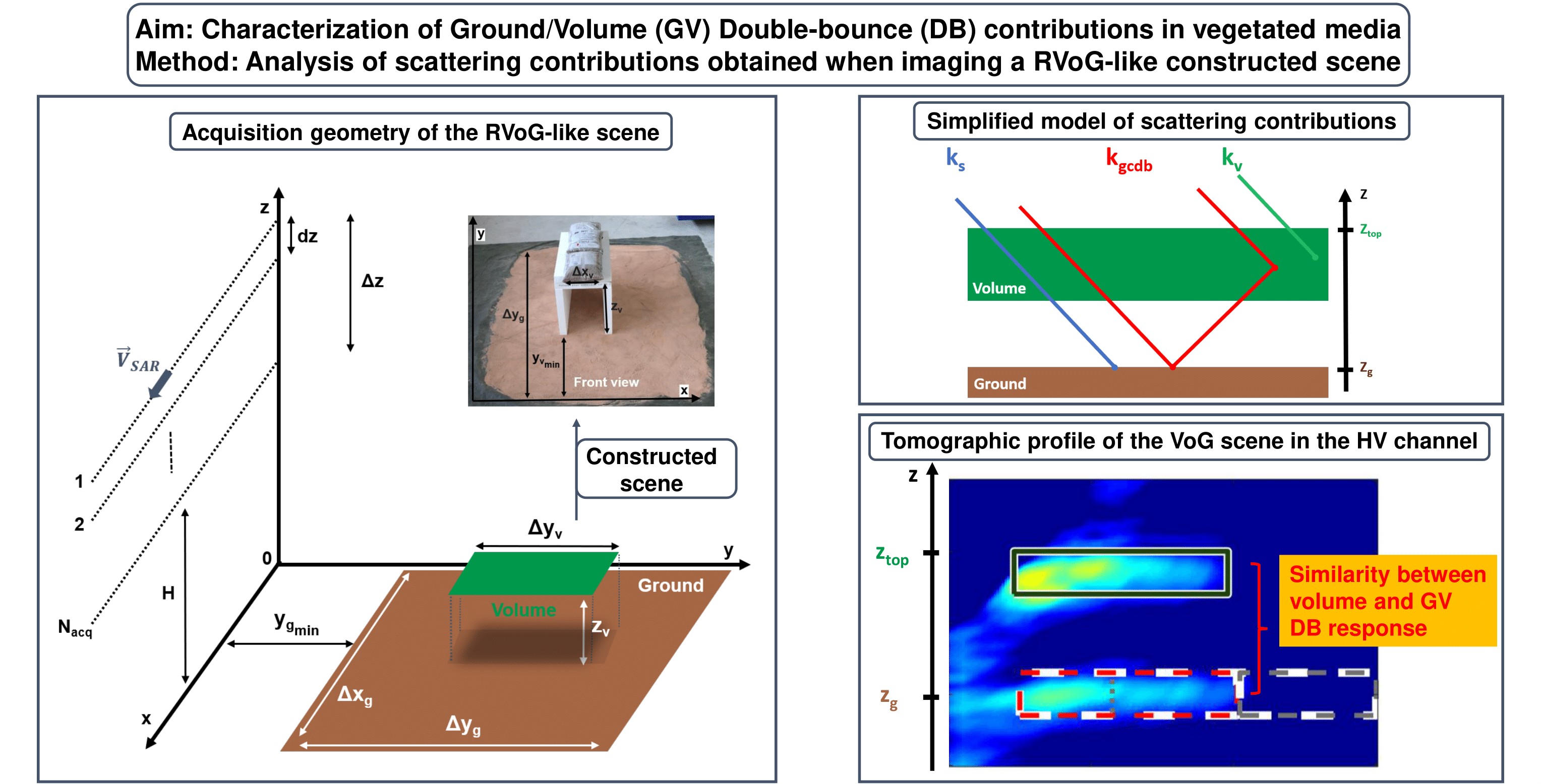
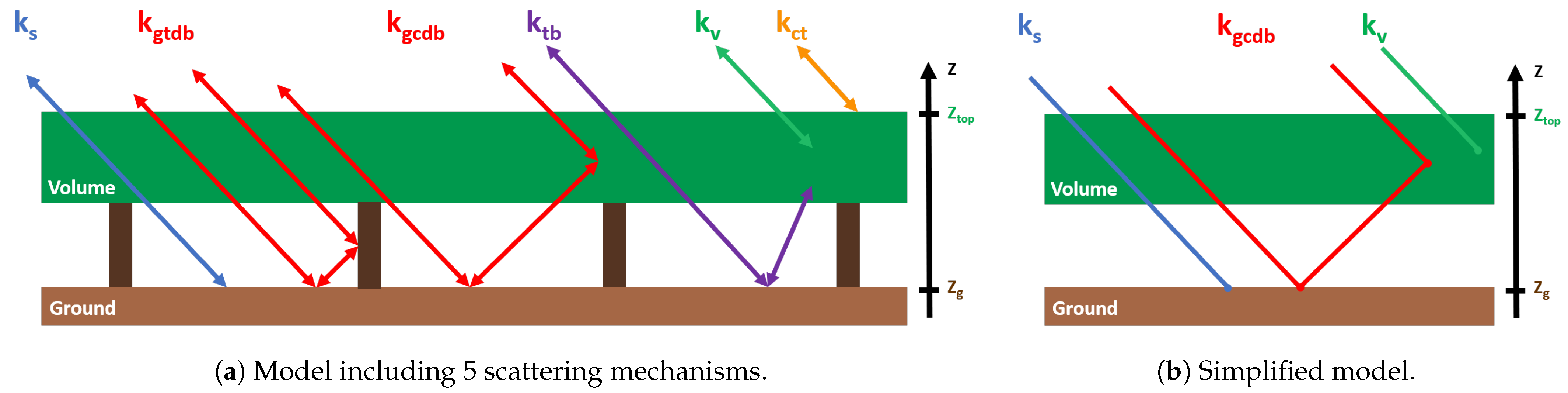
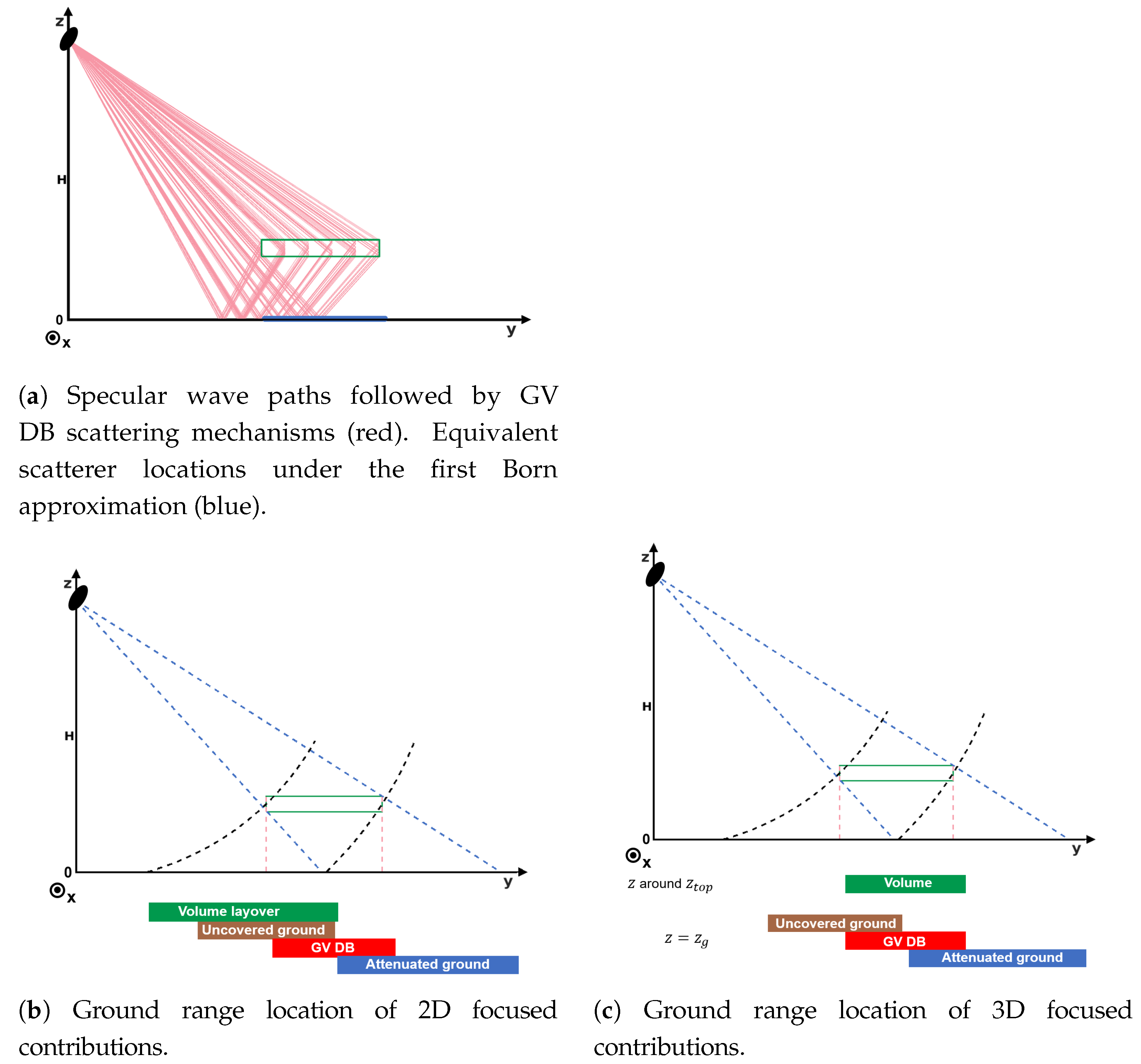
2. Scattering Contributions to the SAR Response of a VoG Scene

The backscattering response of a semi-opaque volume lying over a slightly rough ground, representing the canopy of a forest and its underlying ground, may be modeled, at order 1, using five contributions [16]. As depicted in Figure 1a, these contributions correspond to reflections at the air–volume interface, ${\mathit{k}}_{\mathit{ct}}$, and from the underlying ground, ${\mathit{k}}_{\mathit{s}}$, to direct backscattering from the volume, ${\mathit{k}}_{\mathit{v}}$, and to ground–trunk ${\mathit{k}}_{\mathit{gtdb}}$ and ground-canopy ${\mathit{k}}_{\mathit{gcdb}}$ Double-Bounce (DB) scattering mechanisms, and to triple-bounce interactions between ground and volume, ${\mathit{k}}_{\mathit{tb}}$. The triple-bounce response, ${\mathit{k}}_{\mathit{tb}}$, is generally weak compared to the other components and may be discarded. The reflection of the canopy top, ${\mathit{k}}_{\mathit{ct}}$, is usually neglected when modeling forested areas, due to the diffuse nature of this interface. This contribution may hence be either disregarded or merged with the volume response. This paper focuses on the study of the GV DB scattering mechanism that is generally only partially accounted for in classical approaches aiming to model Polarimetric SAR Interferometric (PolInSAR) and PolTomSAR echoes [17,18,19]. It is a known fact that DB contributions cannot be separated from the soil response using 2D and even 3D imaging processes, and, as a consequence, classical modeling approaches gather reflection on the soil and DB scattering into a single ground contribution. This study proposes to further investigate the influence of DB mechanisms on the features of 2D and 3D images and uses the simplified model given in Figure 1b, which considers a Ground-Volume (GV) DB term in addition to the usual soil and volume responses. The ground–trunk DB interaction, shown in Figure 1a, is a well studied scattering mechanism [20,21,22], known to have a well-localized response and deterministic polarimetric patterns. Hence, an adequate selection of polarization can be implemented in order to filter out such responses. The ground-canopy DB is not well known and is the object of the study performed in this paper, based on a specific configuration, with a volume composed of a canopy only, i.e., without trunks, as illustrated in Figure 1b.

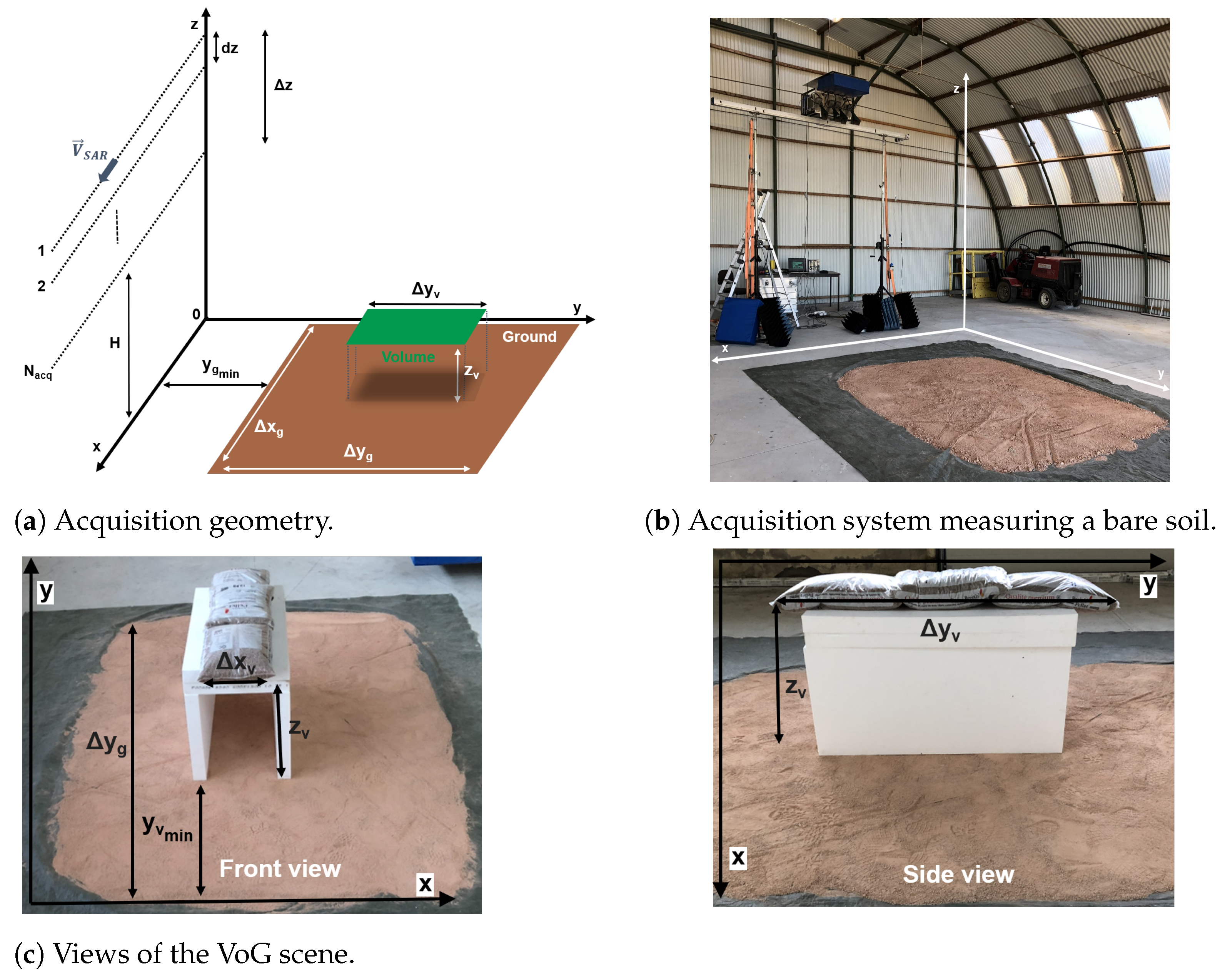
3. Controlled Measurement of a VoG Scene Using a Ground-Based SAR

3.1. Scene and System Configurations

The importance and intrinsic features of the different scattering contributions occurring in the VoG scenario of Figure 1b are assessed using a controlled tomographic imaging experiment, depicted in Figure 2a, where the Cartesian coordinates $(x,y,z)$ denote the azimuth, ground range, and elevation axes, respectively. A small scale scene, composed of a volume lying over a styrofoam prop above a slightly rough ground, is imaged using a Ground-Based (G-B) SAR system developed at the IETR, University of Rennes 1, France, and used in many studies dealing with the characterization of natural volumes [23,24,25].

The system is based on the use of a Vector Network Analyzer (VNA) for the controlled transmission and reception of radar signals. As shown in Figure 2b, the acquisition system, composed of the VNA and four pyramidal horn antennas, is placed on a platform moving along a 3 m-long rail, whose position can be changed using a stepper motor, in order to form a synthetic aperture. The elevation of the rail is controlled by two adjustable vertical poles. The system can operate at different frequency bands, with $f_c\le$ 20 GHz, and over different polarization channels. Each of the four antennas may either be used as a transmitter or a receiver, providing six equivalent monostatic images [23,24,25]. In the frame of this study, the system is operated at X-band, and is fully polarimetric. The main characteristics of the system and of the focused 2D and 3D SAR images are given in

Table 1. System parameters, image features, and scene dimensions.

System Parameters		Image Features		Scene Dimensions
Height	H = 2.99 m	Azimuth resolutions	${\delta }_x$ = 1.75 cm	$y_{g_{min}}$	1.5 m
Carrier frequency	$f_c$ = 10 GHz	Slant range resolutions	${\delta }_{rg}$ = 3.75 cm	${\Delta }_{x_g}$	2.2 m
Bandwidth	B = 4 GHz	Ground range ambiguity	$y_{amb}$ = 6 m	${\Delta }_{y_g}$	3.5 m
Incidence angle	$\theta$ = ${20}^{°}$ to ${60}^{°}$	Vertical resolution	${\delta }_z$ = 0.13 m to 0.22 m	$y_{v_{min}}$	0.96 m
Verical baseline between two consecutive acquisitions	dz = 2 cm	Vertical ambiguity	$z_{amb}$ = 2.96 m to 5 m	${\Delta }_{x_v}$	0.4 m
Number of acquisitions	$N_{acq}$ = 24	Polarization	hh, hv, vv	${\Delta }_{y_v}$	1.5 m
				$z_v$	0.76 m

.

The imaged scene, shown in Figure 2c, is composed of wood pellets for the volume, sand on the ground, and styrofoam as a transparent prop. The dimensions of volume and ground as well as their location in the imaged scene are detailed in Table 1, and are represented in Figure 2. It is important to mention that the ground layer is very shallow, whereas the volume thickness, equal to 0.2 m, is very close to the value of the vertical resolution ${\delta }_z$. The wood pellets used to simulate volume particles consist of small cylinders of compressed dry wood material, whose approximate height and diameter are 25 mm and 6 mm, respectively, as shown in Figure 3.

Wood pellets are patched into 20 cm-thick plastic bags, corresponding to a rather dense equivalent medium, whose volumetric mass is approximately 375 kg/m${}^3$. The volume shown in Figure 3, consisting of dry and randomly oriented wooden cylinders, is expected to behave as a semi-opaque medium with a strongly depolarizing scattering behavior, and whose attenuation does not depend on the incident wave polarization. Unlike natural forest canopies, whose density gradually increases when moving down from the air–canopy interface inside the volume, the proposed volumetric medium presents a sudden transition at the air–volume upper interface, due to the important and uniform density of the pellet heap. Hence, it is very likely that the combined actions of the strong dielectric contrast and the alignment of wood pellets on the bag walls lead to the creation of a significant single-bounce scattering contribution at the air–volume interface, named ${\mathit{k}}_{\mathit{ct}}$ in Figure 1a.

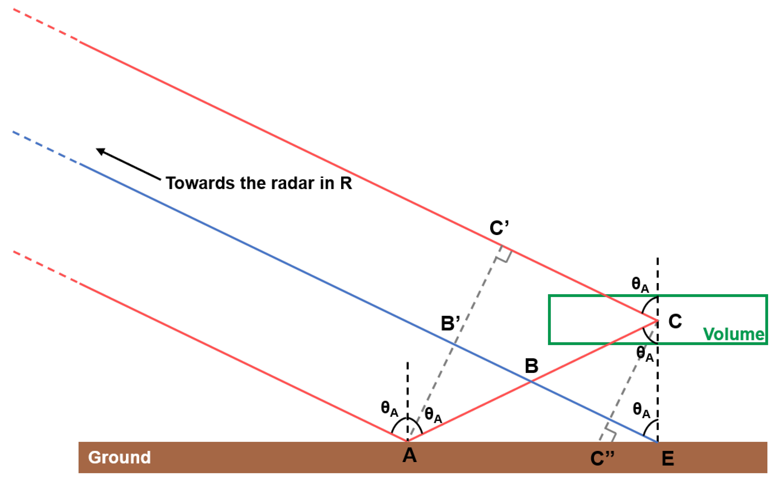
3.2. Imaging Geometry

Classical radar imaging techniques operate under the Born approximation at order 1, which permits to focus range profiles, 2D and 3D images using linear operators. This assumption considers a scene as a sum of scatterers, whose global response is the sum of the individual ones. Scattering phenomena involving multiple wave–matter interactions cannot be handled properly under this simplified linear model, and generally result into equivalent scatterers having modified radiometric and geometrical properties. The DB scattering mechanism provides a nice example of how limitations of the Born approximation at order 1 lead to a modification of the equivalent scene geometry perceived by a radar. The geometrical configuration of DB scattering occurring in the far field of the radar and following specular wave paths is illustrated in Figure 4.

Under the far field hypothesis, the scene is illuminated by the radar using plane waves, and scatters plane waves back to the radar. The restriction of bistatic scattering, occurring over slightly rough surfaces, to specular paths aims to concentrate the analysis onto the most energetic contributions. The path followed by the signal during DB scattering is depicted in Figure 4 using a red plain line. The incident wave reaches location A on the ground under the angle of incidence ${\theta }_A$ and is reflected towards a scatterer of the volume located in C, where another specular reflection sends back the wave to the radar. Under the plane wave hypothesis, the paths between the radar and the locations A and C are parallel and the total distance travelled by a wave following the red path may be expressed using simple considerations [26]. Both triangles $\widehat{AB{B}^{\prime }}$ and $\widehat{AC{C}^{\prime }}$ are isosceles, and one may then deduce that

$$d_{AB}=d_{BE}=d_{BC}$$

(1)

with $d_{XY}$ the distance between locations X and Y. The triangle $\widehat{AC{C}^{\prime }}$ being a rectangled one, the following property may be enounced

$$\frac{d_{B{B}^{\prime }}}{d_{C{C}^{\prime }}}=\frac{d_{AB}}{d_{AC}}$$

(2)

Inserting (1) in (2), one obtains the following expression for the total travelled distance:

$$d=d_{RA}+d_{AC}+d_{C{C}^{\prime }}+d_{R{C}^{\prime }}=2d_{RA}+2d_{AB}+2d_{B{B}^{\prime }}$$

(3)

where $d_{RA}=d_{R{C}^{\prime }}$ stands for the distance travelled by a plane wave between the radar and points A or C’. The two way distance corresponding to the blue path writes as follows:

$$2d_{RE}=2(d_{R{B}^{\prime }}+d_{B{B}^{\prime }}+d_{BE})=2d_{RA}+2d_{AB}+2d_{B{B}^{\prime }}=d$$

(4)

Hence, according to (4), the distance travelled by the wave, or equivalently the radar signal phase history, along the red path is equal to the one occurring along the blue path. The DB scattering mechanism is then, under the first Born approximation, equivalent to an artificial scatterer located in E, i.e., at the ground level elevation and exactly at the ground range position of point C.

The robustness of DB location estimation is also validated considering general spherical waves, as shown in Figure 5a, where red lines illustrate DB scattering paths involving particles located within the volume, and blue dots at ground level, underneath the volume, indicate the equivalent location of DB contributions belonging to the volume.

The ground range locations of the different contributions, in the case of 2D SAR focusing onto a horizontal plane at elevation $z=z_g=0$m, are shown in Figure 5b. The direct return from the volume appears as shifted towards near range, due to the layover effect, which affects the focused response of scatterers whose actual elevation is higher than the one of the focusing plane, as shown in Figure 4 with the scatterer located in C, whose distance to the radar is equal to the one of point C”. GV DB contributions are focused exactly at the volume ground range positions. One may note that, due to the restricted extent of the volume in the ground range direction, ${\delta }_{y_v}$, the GV DB scattering mechanism propagates only once through the volume layer. Depending on the considered ground range coordinates, the ground response may either be attenuated, due to the propagation through the volume, or not, as it occurs over bare ground. Classical 2D SAR images are hence deeply affected by the presence of a volume, with up to three contributions falling within a resolution cell. The locations obtained in the case of 3D SAR imaging, presented in Figure 5c, show that SAR tomography is able to separate, under favorable vertical resolution conditions, the volume response from the echoes located on the ground, and hence resolve the layover ambiguity. Tomographic 3D imaging cannot further unmix the ground and GV DB terms, which appear as focused at $z=z_g$.

3.3. Radiometric Corrections

Images provided by 2D or 3D canonical imaging processes generally represent a significantly distorted estimate of the scene reflectivity. Beyond the limitations of the first Born approximation mentioned above, a SAR image is generally affected by several artifacts, such as spatial variations of the image resolution, and attenuations due to the two-way wave propagation, and to the antenna diagrams. The importance of such effects is illustrated in Figure 6, which shows images before and after the correction of radiometric effects of the polarimetric intensity or span, defined as

$$\mathrm{span}=I_{hh}+2I_{hv}+I_{vv}$$

(5)

The uncompensated 2D image of Figure 6c of the bare soil depicts a reflectivity having a bell shape in the range direction, due to the non flat antenna patterns displayed in Figure 6a. The corresponding compensated image shows a classical diminution of the intensity as the incidence angle value increases. The calibration procedure used in this study is two fold. The first step involves the compensation of the antenna radiation pattern during the focusing process. This factor is applied in order to correct the measured signal according to the position at which imaging is performed. This correction is hence more accurate in 3D image synthesis than for 2D focusing. The second correction aims to compensate coherent processing gains and resolution effects which may affect the intensity of a SAR image. This phase is highly connected to the way SAR focusing is implemented. Intensity distortions are obviously influenced by the geometry of the scene, which remains badly handled by 2D imaging. This fact is documented in Figure 6c,d, which show the effect of compensation performed with the hypothesis of a planar scene, located at $z=z_g=0$ m. Bare soil areas are well corrected, whereas the volume reflectivity is over-compensated, due to the layover effect commented earlier. In the 3D case, radiometric corrections lead to great modifications of the reflectivity map.

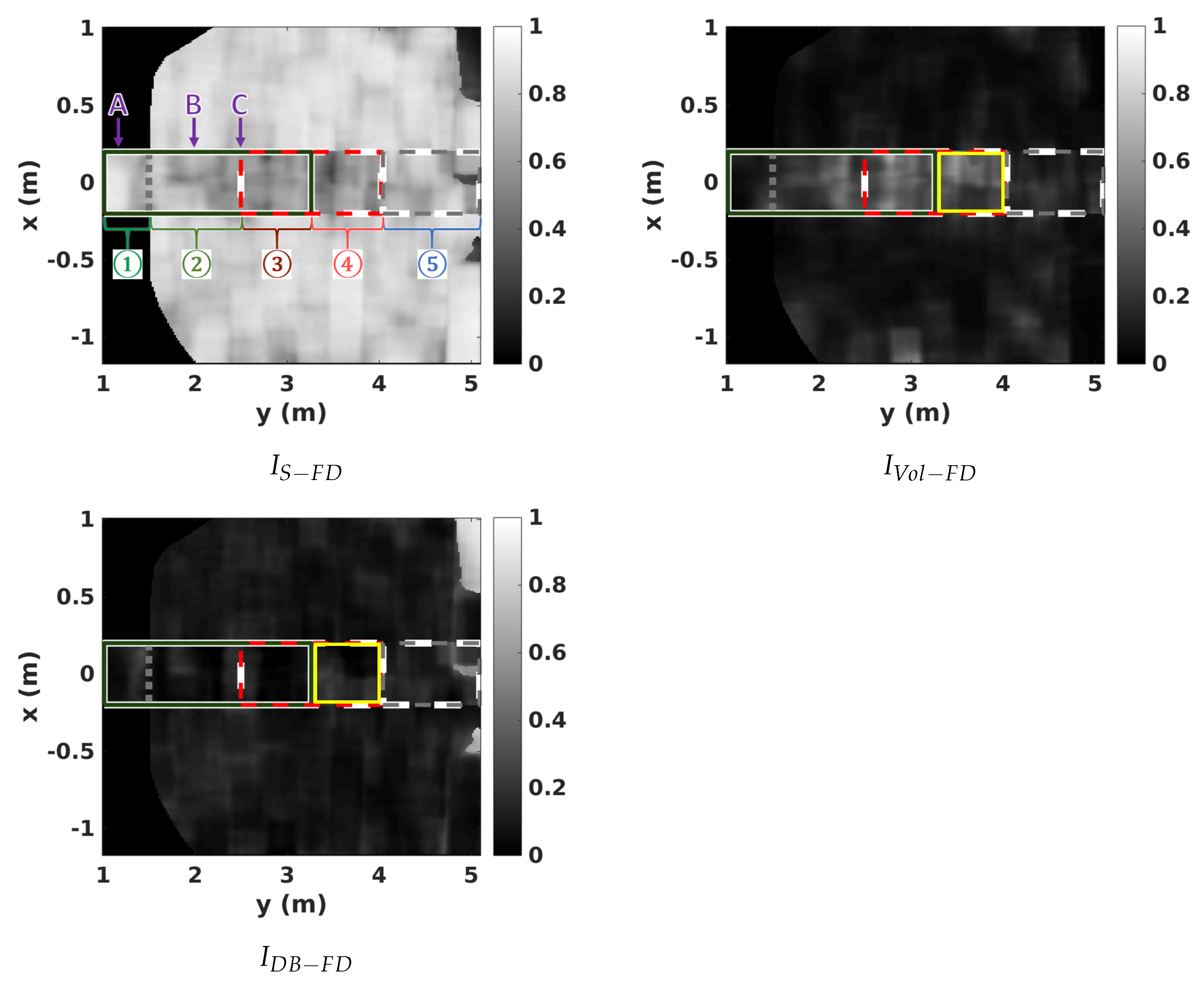
4. 2D SAR Scene Features

Figure 7a and

Table 2. Ground range domains corresponding to the regions indicated in Figure 7a.

Zone Index	①	②	③	④	⑤
Ground range domain	1 m to 1.5 m	1.5 m to 2.46 m	2.46 m to 3.15 m	3.15 m to 3.96 m	3.96 m to 5.1 m

represent the 2D location of the scattering contributions corresponding to the geometrical configuration of the scene described in Figure 2 and Table 1, and for 2D imaging performed in ground range coordinates at $z=z_g=0$m. Five regions, directly derived from Figure 5b, are identified using a numerical index. Zone ① contains volume contributions only, whereas zone ② is composed of a mixture of volume and bare ground responses. Zone ③ presents the most complex scattering features, with a mix of echoes originating from the volume, with GV DB and bare ground contributions. Zone ④ is particularly interesting in this study, as it contains only the GV DB and attenuated ground terms, and may be used to effectively assess the perturbation of the ground response brought by the GV DB mechanism. Zone ⑤ corresponds to the attenuated ground response.

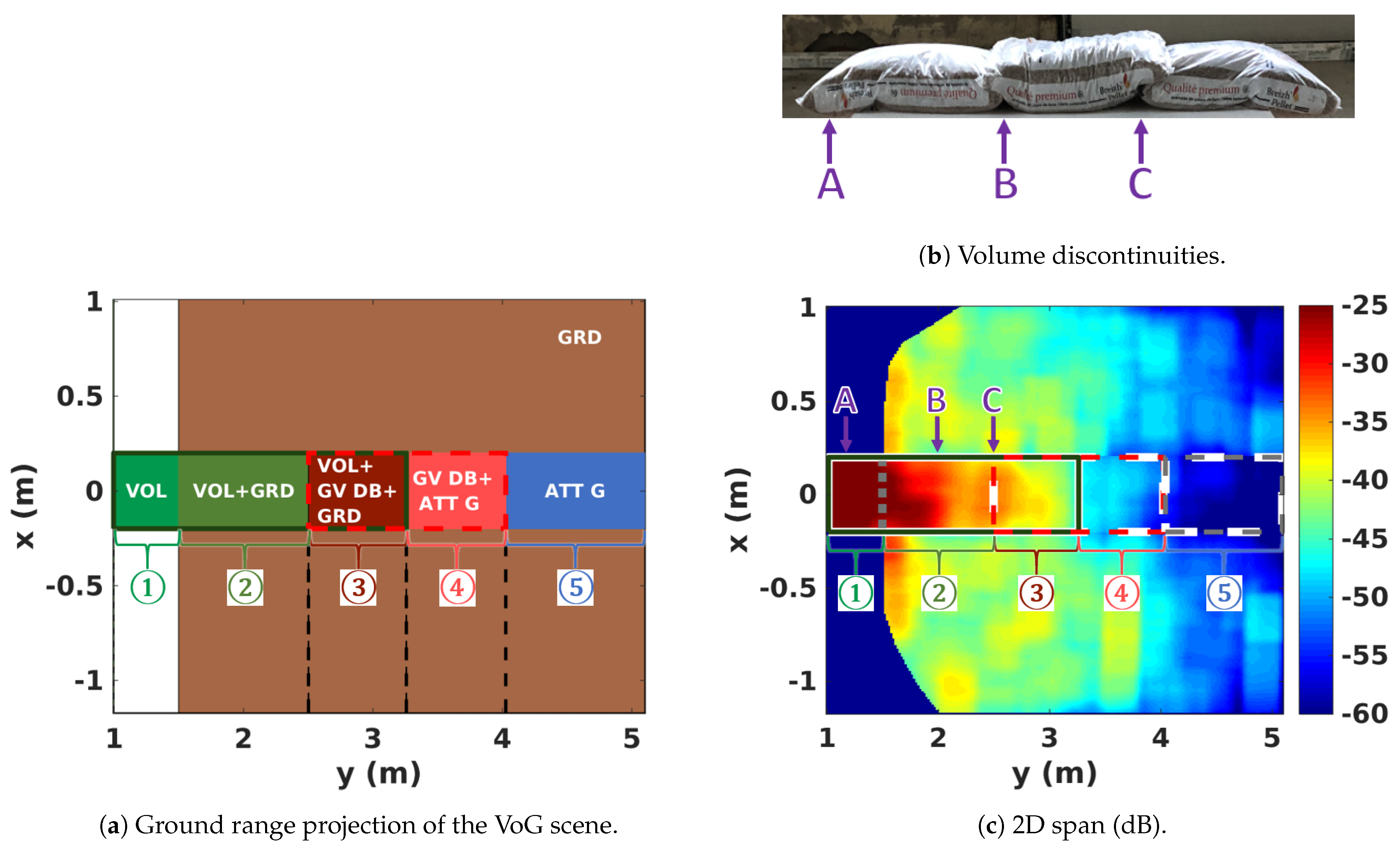
4.1. Interpretation of Reflectivity Patterns

The most striking feature of the 2D span image given in Figure 7c concerns the response of the volume, whose geometrical features are strongly affected by the layover effect. This contribution results into very high reflectivity patterns within regions ① to ③. The significant decrease of intensity of the volume response as ground range increases may be explained by considering both wave scattering physics and 2D imaging geometry. According to the layover effect described above, the volume, whose true position corresponds to incidence angles varying from 42${}^{°}$ up to 57${}^{°}$, appears at ground range coordinates ranging between 1 m and 3.15 m, i.e., with an incidence angle on the ground ranging from 17${}^{°}$ to 44${}^{°}$. The consequence of this mislocation is that echoes measured within an angular domain of [−3${}^{°}$, 12${}^{°}$] in the antenna coordinates, i.e., around 45${}^{°}$, are compensated with values computed from the domain [−28${}^{°}$, −1${}^{°}$], still in the same antenna-centered reference. This misalignment of the measured and compensated domain leads to a strong amplification of the reflectivity in near range and to a pattern that varies rapidly in the range direction. Moreover, the volume being located much closer to the radar in the elevation direction, the resulting strong diversity of incidence angles induces drastic changes of scattering mechanisms as ground range coordinate increases. As explained earlier, it is very likely that the reflection at the air–volume interface reveals itself to be significant, due to the strong dielectric constant between the air and rather dense medium composed of patched wood pellets. It is well known that the intensity of surface reflection can be very sensitive to the incidence angle [27,28], in particular for smooth interfaces. Beyond a given range of incidence angles, the surface reflection becomes negligible and the volume response is then dominated by the diffuse echo of randomly oriented anisotropic wood pellets.

As shown in Figure 7b, the packaging of the wood pellets, used to play the role of a diffusing layer, does not permit to deal with a continuous and homogeneous medium. Three bags have been juxtaposed in order to form a long enough layer, and the unavoidable and undesired discontinuities between the bags can be well perceived in Figure 7c, which shows some variations of the backscattered intensity at the locations corresponding to the discontinuities. GV DB mechanisms may also be directly perceived from Figure 7c with the sudden decrease of intensity between region ④, containing GV DB and attenuated ground contributions, and region ⑤, which corresponds to the attenuated ground only. The significance of the GV DB may also be appreciated by noticing that the reflectivity in region ④ is comparable to the one of the bare ground. Coarse intensity estimates indicate that the level of the GV DB contribution is around –49 dB.

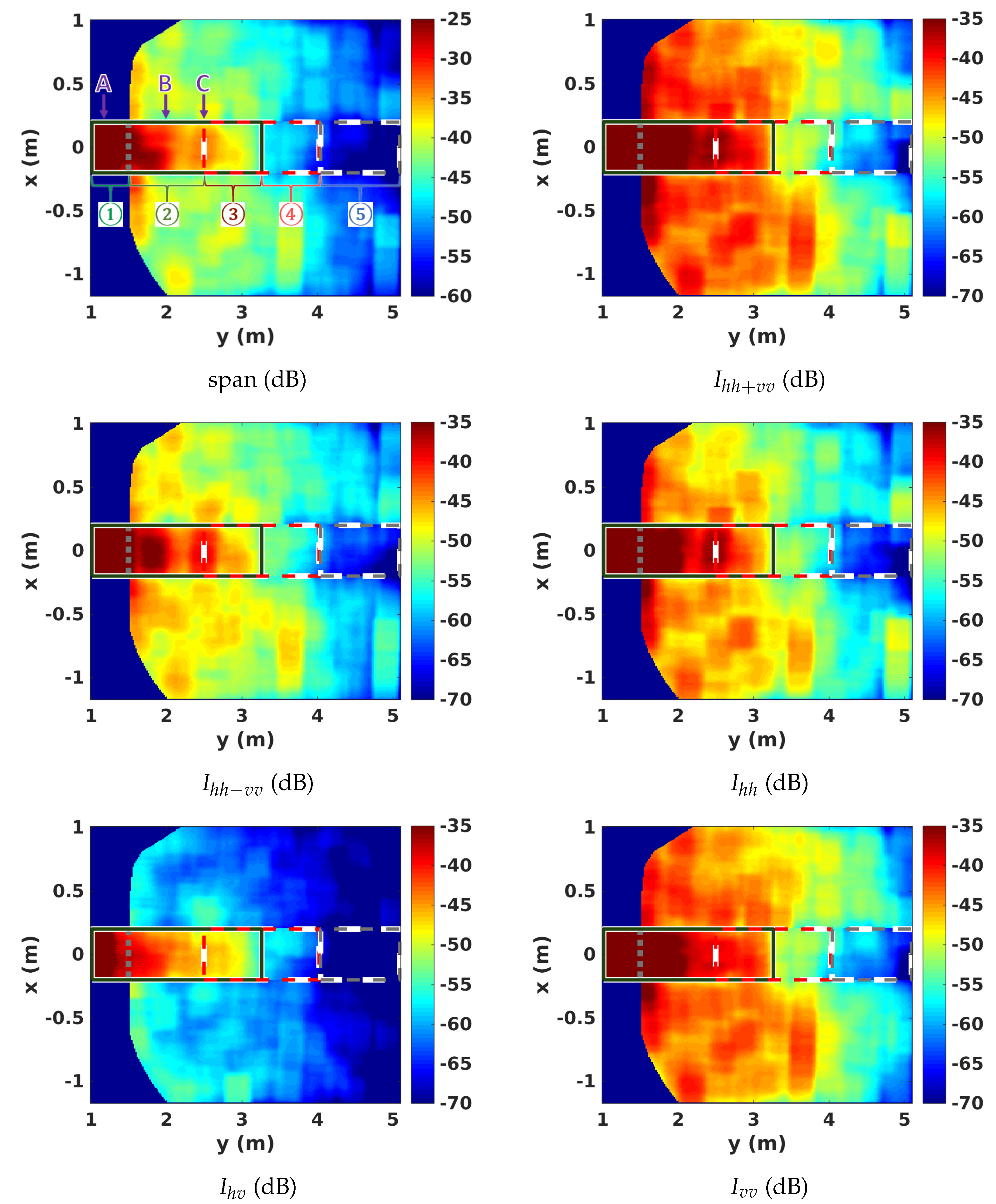
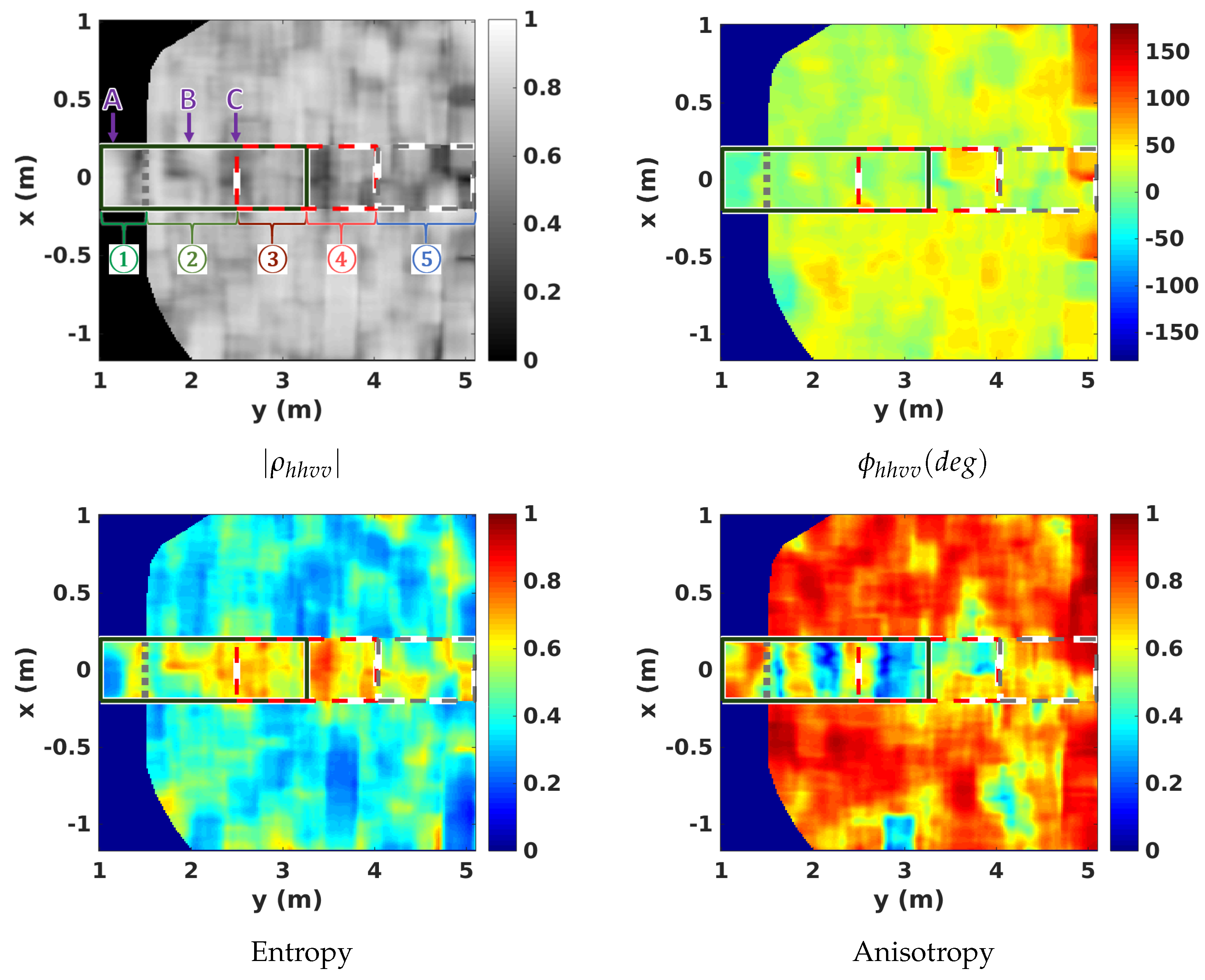
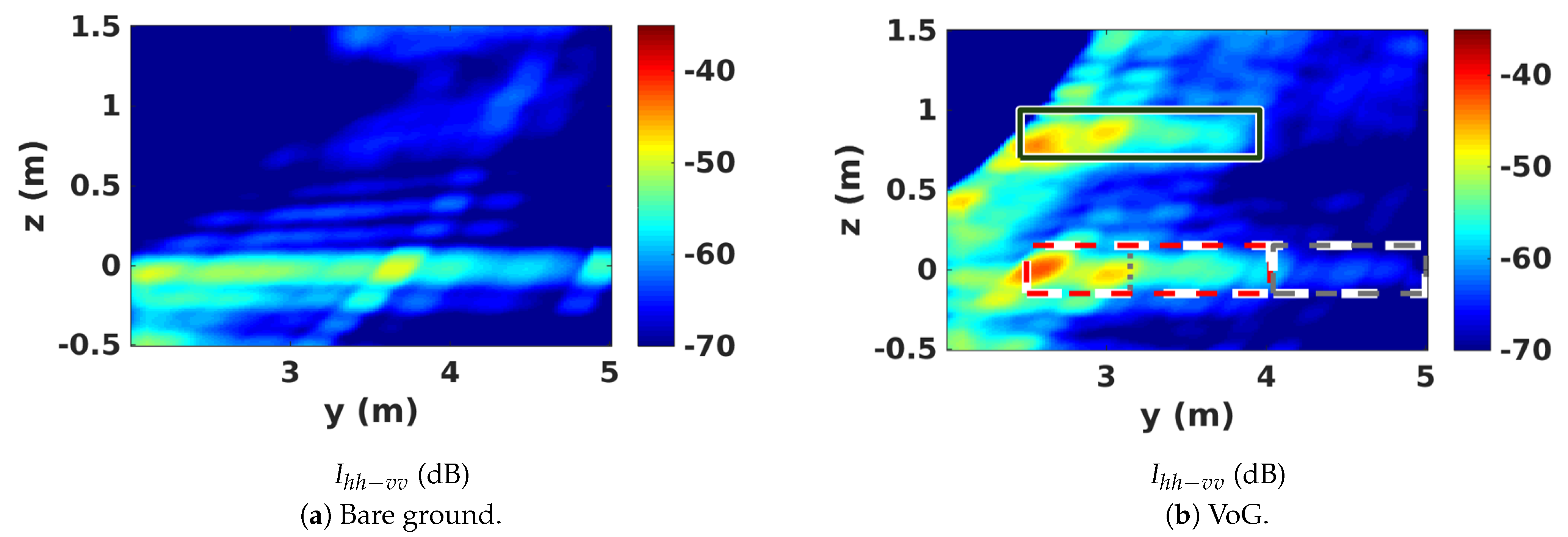
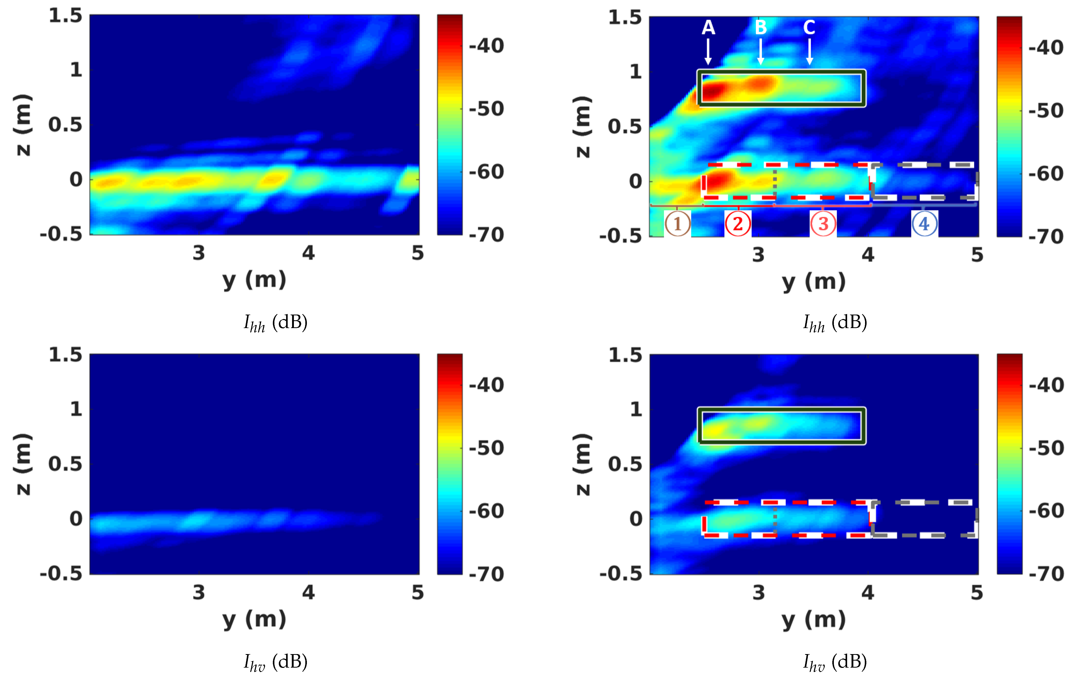
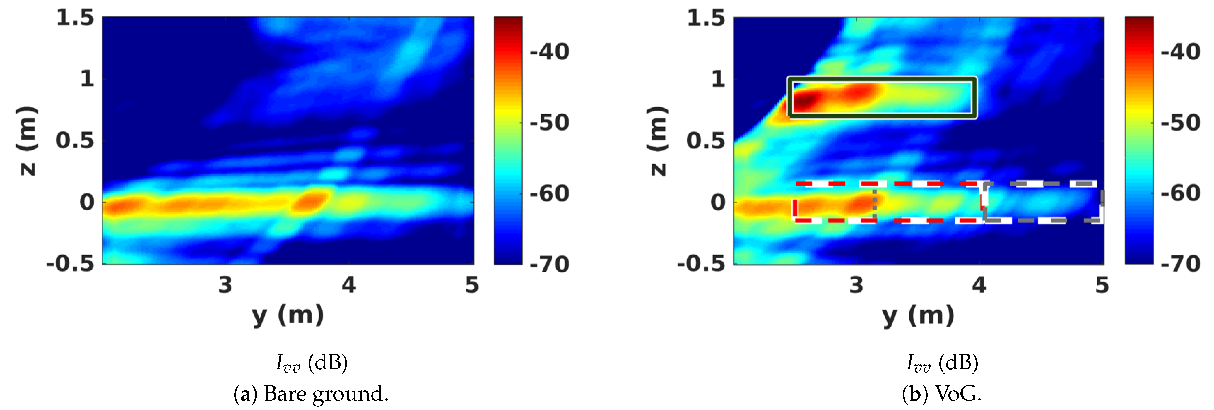
4.2. Polarimetric Analysis

A more refined analysis of the complex scattering patterns of the constructed VoG scene may be conducted from the polarimetric intensities, computed in the Pauli and Lexicographic [29] bases, and shown in Figure 8.

Polarimetric features confirm the preliminary conclusions derived from Figure 7 regarding the significance of the GV DB scattering mechanism. Indeed, according to the classical modeling approaches presented in [20,21,22], in the absence of DB wave interactions between the ground and tree trunks, the variation of intensity between regions ④ and ⑤ should be much smaller, and similar to the trend observed over the bare soil area surrounding the artificial volume. A similar observation may be made regarding the similar level of reflectivity observed over region ④ and over the ground observed under the same incidence angle. Again, region ④ should exhibit a much smaller reflectivity in all polarimetric channels. This departure from a scattering behavior that is well predicted by classical approaches is obviously due to the presence of GV DB, whose effect is particularly noticeable in the hv channel. One may note that, despite the fact that GV DB involves two consecutive forward wave reflections, the corresponding responses cannot be clearly identified as a DB by comparing $I_{hh-vv}$ and $I_{hh+vv}$, as this is done in the literature. In the present case, $I_{hh-vv}$ is significantly lower than $I_{hh+vv}$, it is also slightly smaller in region ④. If some of the scattering patterns created by the discontinuities of the volumetric mechanism displayed in Figure 7 may be perceived to be reliable conclusions that cannot be formulated, as such heterogeneities may significantly contribute to double-bounce scattering mechanisms, occurring at ground range positions different from those given in Figure 8, which only account for the layover effect. The polarimetric indicators shown in Figure 9 may be used to further characterize the studied GV DB scattering term. The images of the normalized correlation coefficient between the co-polarized channels, ${\rho }_{hhvv}$, show that the GV DB does not behave as a classical DB scattering mechanism, as the phase difference between hh and vv channels remains close to 0. Moreover, the low values taken by $|{\rho }_{hhvv}|$ over region ④ in which the GV DB is known to dominate the global responses may be associated with a volume-like scattering term, as defined in various models, such as [30].

The entropy parameter, defined in [29,31] as an indicator of the degree of polarimetric randomness, and computed using the eigenvalues of the polarimetric covariance matrix, confirms this interpretation. The ground response may be considered as polarimetrically deterministic, with a single dominant unitary rank scattering term, whereas the layover area and region ④ show significantly larger steep values. The GV DB is found to reach the highest entropy values due to a continuation of co-polar decorrelation with the presence of a significant return in the hv channel. The anisotropy, describing the relative importance of scattering mechanisms, is more affected by the scattering artifacts associated with the discontinuities shown in Figure 7b.

The results of the Freeman–Durden decomposition [30] given in Figure 10 indicate that GV DB scattering does not behave as a classical double-bounce interaction, and that it may be assimilated to volume diffusion, as $I_{Vol-FD}$ has significant values over regions ③ and ④ only. One may note here that, due to technological limitations, related to the density of the volume ersatz used in this study, scattering in the layover region is not dominated by volume diffusion, but rather by surface scattering at the volume top interface. Nevertheless, the GV DB term shows volume-like scattering features. Having to lead this analysis with 2D SAR images represents a limitation, such as in region ③, within which GV DB echoes cannot be separated from the volume layover, and, moreover, the relationship between GV DB and volumetric contributions cannot be clearly established. In such structures, 3D imaging using SAR tomography represents a very appealing solution and is studied in the following.

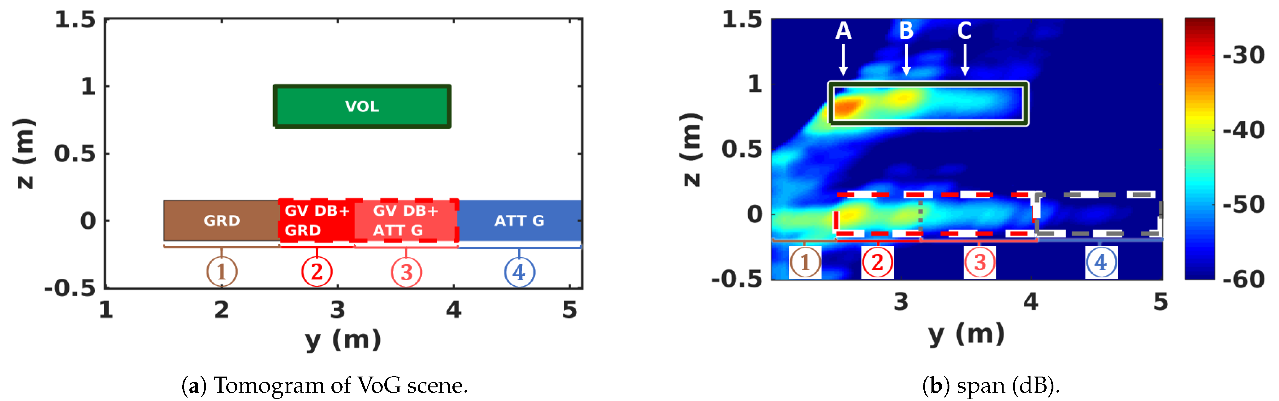
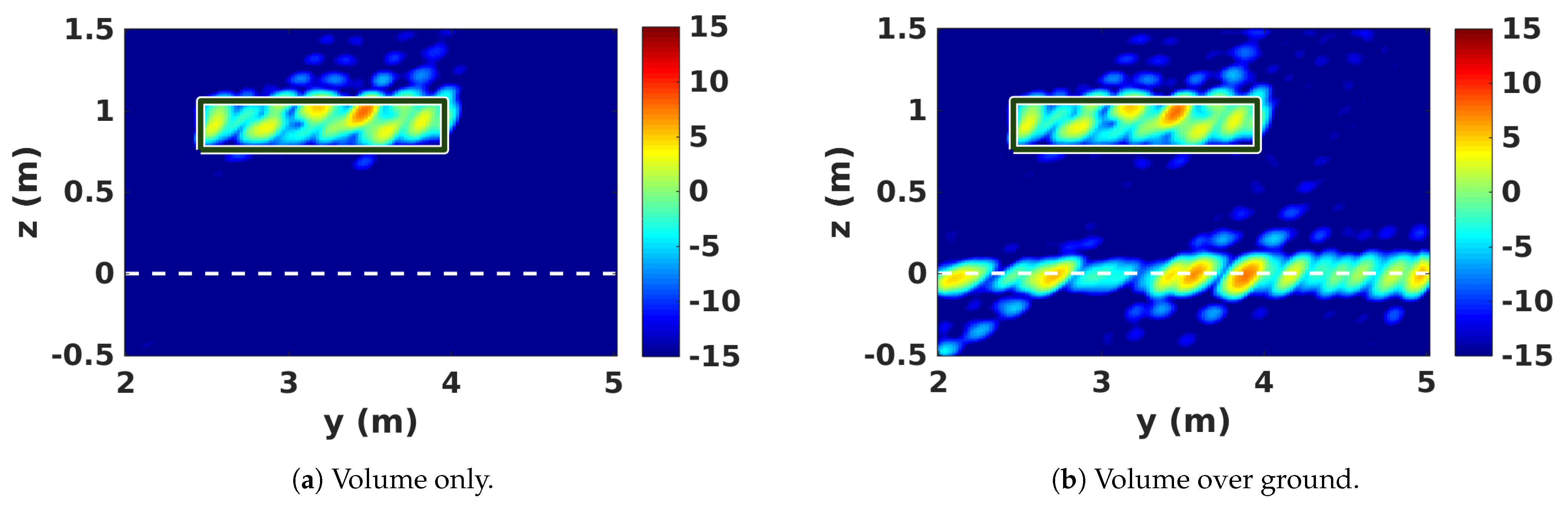
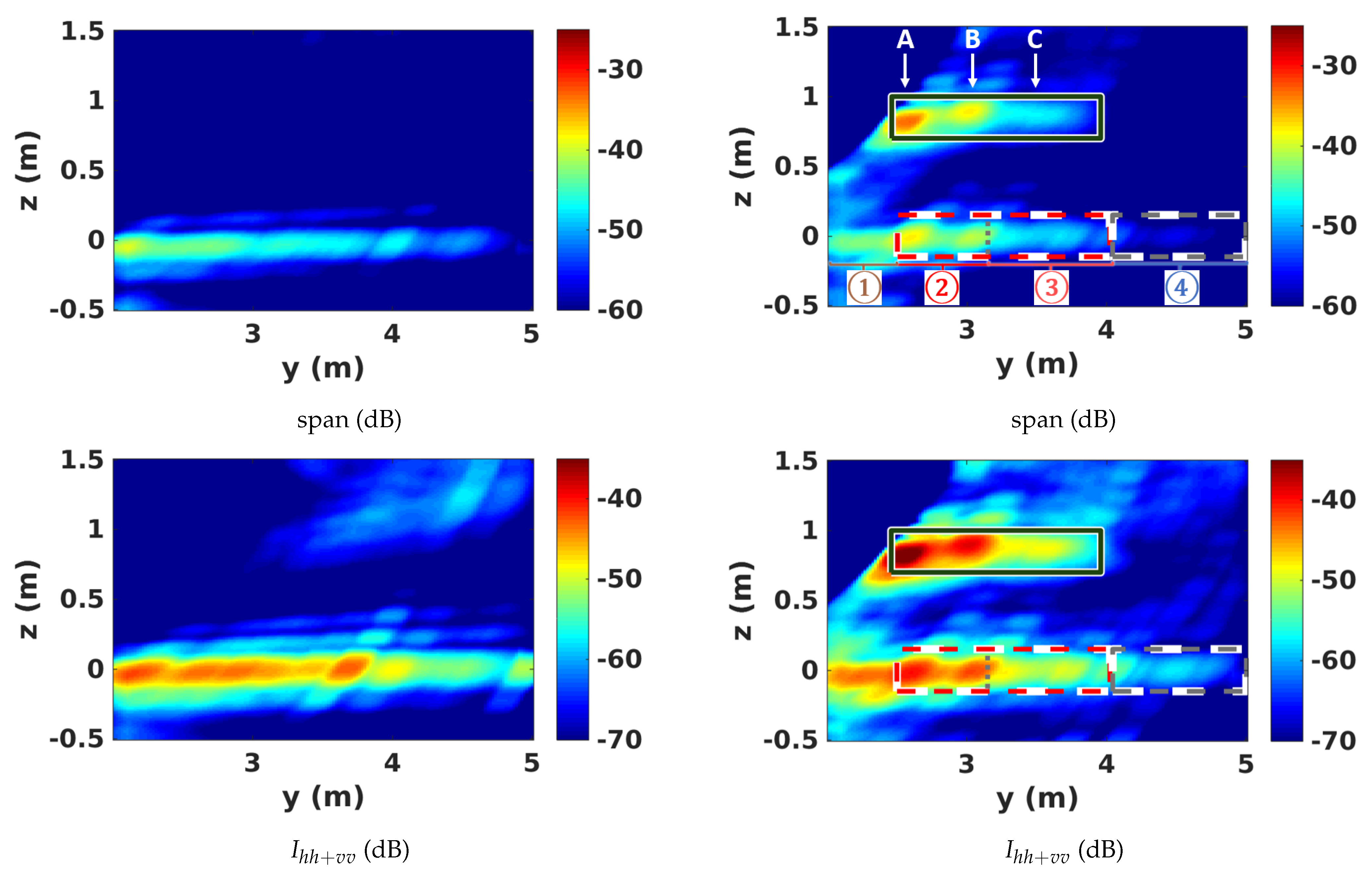
5. 3D SAR Scene Features

5.1. Location of Scattering Contributions in 3D SAR Images

As this is clearly shown in Figure 5c, the ability of 3D SAR imaging for separating volume scattering from ground contributions is crucial for the analysis of the underlying soil properties. Nevertheless, the presence of a GV DB component, whose 3D location remains at the ground level, may limit this characterization. Assuming that volume and ground terms are perfectly separated during tomographic focusing, one may consider four regions at ground level, represented using indexed zones in Figure 11a.

The quality of the spatial separation brought by 3D focusing, which may play an important role in this analysis, can be assessed by considering the vertical resolution and also the shape and side-lobe levels of the vertical ambiguity function.

The tomographic acquisitions considered in this study are performed using wide band signals and performed in near field configuration. Thus, providing an analytical expression of the 2D vertical ambiguity function, h(y,z) reveals to be particularly difficult. The assessment of ground and volume separation is hence conducted using a simple simulation of the 3D imaging of a volume lying above a ground, whose results are presented in Figure 12. Simulation results show that the effective vertical resolution is well adapted to the configuration under study, with ground and volume components having comparable reflectivity values, as shown in Figure 12. The study of the volume alone shows that 3D focusing provides an isolation of around 28 dB, which one may consider as a reasonable level of decoupling. As a consequence, volume and ground components are well separated in the present configuration, and the use of further separation strategies, such as the one based on polarimetric diversity as proposed in [1], is not necessary.

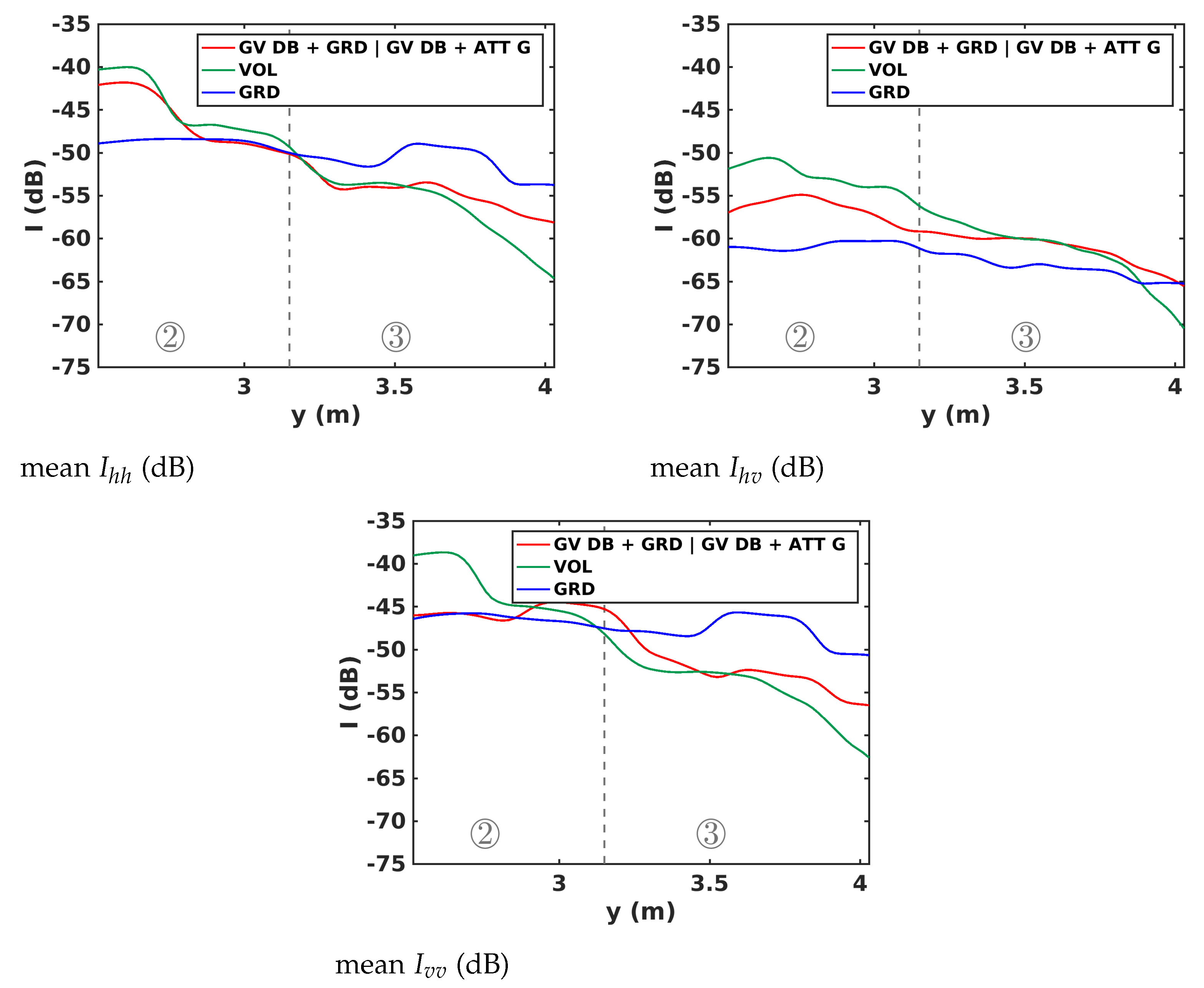
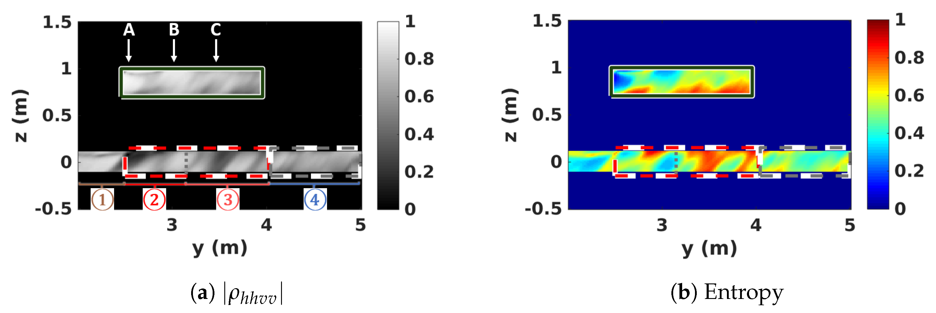
5.2. 3D Polarimetric Analysis

The 3D polarimetric radiometric features displayed in Figure 13 and Figure 14 permit a much clearer and deeper analysis than their 2D counterparts. Indeed, 3D focusing performed at high-resolution efficiently removes the layover and provides unambiguous access to the responses located at the ground level. The images given in Figure 13 and Figure 14 compare tomographic profiles obtained over bare ground and in the VoG scene for different polarimetric channels.

The most obvious observation that can be raised concerning these radiometric features regards the similarity between the profile of the volume, located around $z_v=0.86$m, and the one measured on the ground, with features that are mirrored from one elevation to the other. This very strong similarity is clearly due to the presence of the GV DB scattering, whose intensity is highly related to the one backscattered by the volume. It may be noted that this resemblance between the profiles affects all the polarimetric channels including the cross-polarized one, hv, whose value below the volume is much larger than the one observed over bare ground. The ground images of the different volume discontinuities do not have equal scattering behaviors. Indeed, the ground image of the discontinuity in A shows a very low value in the vv channel, and very close $I_{hh+vv}$ and $I_{hh-vv}$ levels. This may be explained by taking into account that the front of the wooden pellet bag may behave like a horizontal dipole having a very low scattering coefficient in the vertical polarization.

The correlation between the volume and GV DB scattering is clearly observed in the mean intensity profiles displayed in Figure 15, whereas the polarimetric features in Figure 16 confirm the conclusions of the 2D analysis. Figure 15 only illustrates intensity variations in regions ② and ③, where GV DB contributions are known to dominate. This figure confirms that the GV DB scattering mechanism is indeed an image of the volume on the ground level, as seen in the hv channel, but can also partially reflect ground response such as in the hh and vv channels. As previously mentioned, region ③ in Figure 16 provides the same polarimetric features as in 2D imaging as it is not affected by the volume layover effect. Since the polarimetric ground images of the volume discontinuities do not behave in the same way, it is hence expected that their resulting polarimetric features will also behave differently. Nevertheless, one can appreciate the rise in the decorrelation of $|{\rho }_{hhvv}|$ and entropy values, on both the volume and its ground image, as ground range increases.

6. Underlying Ground Characterization

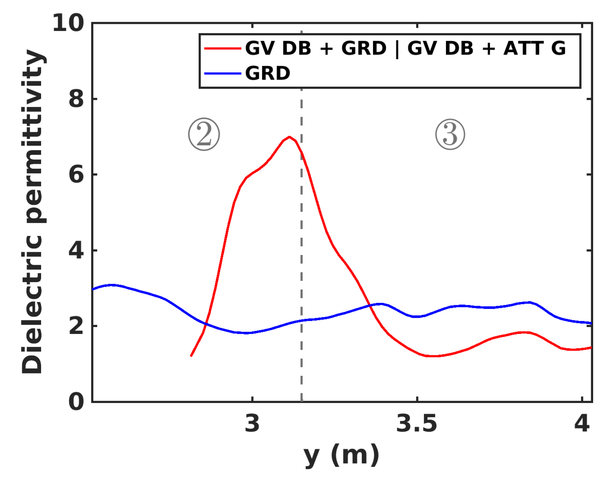
6.1. Dielectric Permittivity Estimation

The importance and the nuisance caused by the GV DB scattering are assessed through the estimation of the ground dielectric permittivity. This estimation uses a surface scattering model based on the Small Perturbation Method [27,32], whose conditions of application agree with the configuration of the studied experiment, and which offers a highly simplifying property of separable sensitivities to dielectric and roughness properties. The dielectric permittivity is hence estimated using the ratio $I_{hh}/I_{vv}$.

The results given in Figure 17 clearly show the impact of GV DB contributions on the estimation of the dielectric permittivity, with values estimated for the underlying ground that are very different than those obtained for bare soil. Region ② contains discontinuities that impact the estimation of the dielectric permettivity due to their polarimetric behavior, which explains the high value found at the discontinuity in B. Nevertheless, region ③ clearly shows an underestimation of this parameter due to the impact of GV DB contributions.

6.2. Ground Polarimetric Features

The mean co-polarized correlation coefficient profile presented in Figure 18a shows a clear decorrelation of the underlying ground, regardless of the discontinuity of the volume. Bare ground values are fairly stable, whereas the volume and its underlying ground have steep variations.

Moreover, a comparison between this parameter and the entropy obtained in Figure 18b shows variations having opposite trends, confirming the conclusions drawn in 2D and 3D analyses.

A similar conclusion may be drawn regarding the mean intensity profile of the Freeman–Durden decomposition given in Figure 19. The identified classical DB component is clearly very low, and region ③ is mostly associated with the volume component.

7. Discussion

The goal of this experiment is to show that the GV DB scattering mechanism is a significant component of the total response of a volume lying over a ground. Indeed, it has been shown that the interfering volume contributions on ground level are not due to the vertical resolution but to the presence of the GV DB scattering mechanism, which cannot be separated from the ground contribution using either 2D or 3D focusing techniques. Despite its DB nature, this scattering mechanism does not behave as planned by classical characterization approaches [30,33], but may be interpreted as a projection of a function of the volume response on the ground, and hence makes the analysis of the underlying ground highly problematic.

These observations are essential when modeling complex environments or handling data acquired over forested areas as the contributions of this volume-like DB scattering are projected on ground level underneath the entire volume. This experiment furthers our understanding of the total ground response lying below a volume and will allow a better assessment and characterization of forest parameters.

8. Conclusions

In this paper, a miniaturized volume over ground scene is imaged with PolTomSAR imaging at high-resolution using a G-B SAR system operated at X-band. The ground consists of a low roughness layer of sand, and the volume consists of wood pellets patched into bags, which are elevated using styrofoam props. The purpose of this constructed scene is to highlight the presence and intrinsic features of the GV DB scattering contributions embedded the response of a forest.

It is shown that the DB scattering mechanism is focused at ground level and exactly underneath the volume, and, by comparing bare ground response or attenuated ground response, with the total underlying ground response, the high amount of influence of GV DB scattering contributions is easily identified in 2D images for all polarimetric channels, and especially in the HV channel where the intensity of the underlying attenuated ground response, containing GV DB contributions, is even higher than the one of bare ground response. However, due to the volume layover effects, PolTomSAR acquisitions are found to be crucial in this study since, using high 3D resolution and a sufficient distance in elevation between ground and volume, the two scattering layers in the scene are efficiently separated, whereas GV DB contributions remain at ground level. It is demonstrated that the underlying ground response is very close to the volume one, due to GV DB contributions. The underlying ground is found to show a decorrelation between the co-polared channels, provides a high entropy, and its dielectric permittivity is badly estimated compared to the one obtained over the bare ground. Moreover, the Freeman–Durden decomposition fails to identify GV DB contributions as classical DB components, but, instead, associates these contributions with the volume component.

This study suggests that a proper characterization of the ground lying below a volume is not only and simply related to the spatial separation of the volume and ground responses, but is affected by a complex mixing governed by the correlation of the backscattering of the ground and the bistatic reflectivity patterns over the volume.

References

1. Tebaldini, S. Algebraic Synthesis of Forest Scenarios From Multibaseline PolInSAR Data. IEEE Trans. Geosci. Remote Sens. 2009, 47, 4132–4142. [Google Scholar] [CrossRef]
2. Tebaldini, S. Single and Multipolarimetric SAR Tomography of Forested Areas: A Parametric Approach. IEEE Trans. Geosci. Remote Sens. 2010, 48, 2375–2387. [Google Scholar] [CrossRef]
3. Tebaldini, S.; Rocca, F. Multibaseline Polarimetric SAR Tomography of a Boreal Forest at P- and L-Bands. IEEE Trans. Geosci. Remote Sens. 2012, 50, 232–246. [Google Scholar] [CrossRef]
4. Huang, Y.; Ferro-Famil, L.; Lardeux, C. Polarimetric SAR tomography of tropical forests at P-Band. In Proceedings of the 2011 IEEE International Geoscience and Remote Sensing Symposium, Vancouver, BC, Canada, 24–29 July 2011; pp. 1373–1376. [Google Scholar]
5. El Hajj Chehade, B.; Ferro-Famil, L. P-band polarimetric SAR tomography for tropical forest structure characterization. In Proceedings of the 2014 11th European Radar Conference, Rome, Italy, 8–10 October 2014; pp. 49–52. [Google Scholar] [CrossRef]
6. Ho Tong Minh, D.; Toan, T.L.; Rocca, F.; Tebaldini, S.; d’Alessandro, M.M.; Villard, L. Relating P-Band Synthetic Aperture Radar Tomography to Tropical Forest Biomass. IEEE Trans. Geosci. Remote Sens. 2014, 52, 967–979. [Google Scholar] [CrossRef]
7. Ferro-Famil, L.; Huang, Y.; Pottier, E. Principles and Applications of Polarimetric SAR Tomography for the Characterization of Complex Environments. In International Association of Geodesy Symposia, Proceedings of the VIII Hotine-Marussi Symposium on Mathematical Geodesy, Rome, Italy, 17–21 June 2013; Sneeuw, N., Novàk, P., Crespi, M., Sansò, F., Eds.; Springer: Berlin/Heidelberg, Germany, 2015; Volume 142. [Google Scholar] [CrossRef]
8. Kugler, F.; Lee, S.; Hajnsek, I.; Papathanassiou, K.P. Forest Height Estimation by Means of Pol-InSAR Data Inversion: The Role of the Vertical Wavenumber. IEEE Trans. Geosci. Remote Sens. 2015, 53, 5294–5311. [Google Scholar] [CrossRef]
9. Ho Tong Minh, D.; Tebaldini, S.; Rocca, F.; Le Toan, T.; Villard, L.; Dubois-Fernandez, P.C. Capabilities of BIOMASS Tomography for Investigating Tropical Forests. IEEE Trans. Geosci. Remote Sens. 2015, 53, 965–975. [Google Scholar] [CrossRef]
10. Ho Tong Minh, D.; Tebaldini, S.; Rocca, F.; Le Toan, T. The Impact of Temporal Decorrelation on BIOMASS Tomography of Tropical Forests. IEEE Geosci. Remote Sens. Lett. 2015, 12, 1297–1301. [Google Scholar] [CrossRef]
11. Pardini, M.; Papathanassiou, K. On the Estimation of Ground and Volume Polarimetric Covariances in Forest Scenarios with SAR Tomography. IEEE Geosci. Remote Sens. Lett. 2017, 14, 1860–1864. [Google Scholar] [CrossRef]
12. Joerg, H.; Pardini, M.; Hajnsek, I.; Papathanassiou, K.P. On the Separation of Ground and Volume Scattering Using Multibaseline SAR Data. IEEE Geosci. Remote Sens. Lett. 2017, 14, 1570–1574. [Google Scholar] [CrossRef]
13. Blomberg, E.; Ferro-Famil, L.; Soja, M.J.; Ulander, L.M.H.; Tebaldini, S. Forest Biomass Retrieval From L-Band SAR Using Tomographic Ground Backscatter Removal. IEEE Geosci. Remote Sens. Lett. 2018, 15, 1030–1034. [Google Scholar] [CrossRef]
14. Mariotti D’Alessandro, M.; Tebaldini, S. Digital Terrain Model Retrieval in Tropical Forests Through P-Band SAR Tomography. IEEE Trans. Geosci. Remote Sens. 2019, 57, 6774–6781. [Google Scholar] [CrossRef]
15. Aghababaei, H.; Ferraioli, G.; Ferro-Famil, L.; Huang, Y.; Mariotti D’Alessandro, M.; Pascazio, V.; Schirinzi, G.; Tebaldini, S. Forest SAR Tomography: Principles and Applications. IEEE Geosci. Remote Sens. Mag. 2020, 8, 30–45. [Google Scholar] [CrossRef]
16. Ulaby, F.; Moore, R.; Fung, A. Microwave Remote Sensing: Active and Passive; Number v. 3 in Artech House Microwave Library; Artech House: Norwood, MA, USA, 1981. [Google Scholar]
17. Papathanassiou, K.P.; Cloude, S.R. Single-baseline polarimetric SAR interferometry. IEEE Trans. Geosci. Remote Sens. 2001, 39, 2352–2363. [Google Scholar] [CrossRef]
18. Cloude, S.R.; Papathanassiou, K.P. Polarimetric SAR interferometry. IEEE Trans. Geosci. Remote Sens. 1998, 36, 1551–1565. [Google Scholar] [CrossRef]
19. Treuhaft, R.N.; Madsen, S.N.; Moghaddam, M.; van Zyl, J.J. Vegetation characteristics and underlying topography from interferometric radar. Radio Sci. 1996, 31, 1449–1485. [Google Scholar] [CrossRef]
20. Dahon, C.; Ferro-Famil, L.; Titin-Schnaider, C.; Pottier, E. Computing the double-bounce reflection coherent effect in an incoherent electromagnetic scattering model. IEEE Geosci. Remote Sens. Lett. 2006, 3, 241–245. [Google Scholar] [CrossRef]
21. Thirion, L.; Colin, E.; Dahon, C. Capabilities of a forest coherent scattering model applied to radiometry, interferometry, and polarimetry at P- and L-band. IEEE Trans. Geosci. Remote Sens. 2006, 44, 849–862. [Google Scholar] [CrossRef]
22. Lin, Y.C.; Sarabandi, K. A Monte Carlo coherent scattering model for forest canopies using fractal-generated trees. IEEE Trans. Geosci. Remote Sens. 1999, 37, 440–451. [Google Scholar] [CrossRef]
23. Yitayew, T.G.; Ferro-Famil, L.; Eltoft, T.; Tebaldini, S. Lake and Fjord Ice Imaging Using a Multifrequency Ground-Based Tomographic SAR System. IEEE J. Sel. Top. Appl. Earth Obs. Remote Sens. 2017, 10, 4457–4468. [Google Scholar] [CrossRef]
24. Yitayew, T.G.; Ferro-Famil, L.; Eltoft, T.; Tebaldini, S. Tomographic Imaging of Fjord Ice Using a Very High Resolution Ground-Based SAR System. IEEE Trans. Geosci. Remote Sens. 2017, 55, 698–714. [Google Scholar] [CrossRef]
25. Rekioua, B.; Davy, M.; Ferro-Famil, L.; Tebaldini, S. Snowpack permittivity profile retrieval from tomographic SAR data. Comptes Rendus Phys. 2017, 18, 57–65. [Google Scholar] [CrossRef]
26. Villard, L.; Borderies, P. On the use of virtual ground scatterers to localize double and triple bounce scattering mechanisms for bistatic SAR. J. Electromagn. Waves Appl. 2015, 29, 626–635. [Google Scholar] [CrossRef]
27. Ulaby, F.T.; Kouyate, F.; Fung, A.K.; Sieber, A.J. A backscatter model for a randomly perturbed periodic surface. IEEE Trans. Geosci. Remote Sens. 1982, GE-20, 518–528. [Google Scholar] [CrossRef]
28. Tsang, L.; Kong, J.A.; Shin, R.T. Theory of Microwave Remote Sensing; A Wiley-Interscience Publication; Wiley: New York, NY, USA, 1985. [Google Scholar]
29. Cloude, S.R.; Pottier, E. A review of target decomposition theorems in radar polarimetry. IEEE Trans. Geosci. Remote Sens. 1996, 34, 498–518. [Google Scholar] [CrossRef]
30. Freeman, A.; Durden, S.L. A three-component scattering model for polarimetric SAR data. IEEE Trans. Geosci. Remote Sens. 1998, 36, 963–973. [Google Scholar] [CrossRef]
31. Cloude, S.R.; Pottier, E. An entropy based classification scheme for land applications of polarimetric SAR. IEEE Trans. Geosci. Remote Sens. 1997, 35, 68–78. [Google Scholar] [CrossRef]
32. Valenzuela, G. Depolarization of EM waves by slightly rough surfaces. IEEE Trans. Antennas Propag. 1967, 15, 552–557. [Google Scholar] [CrossRef]
33. Cloude, S.R.; Pottier, E. Concept of polarization entropy in optical scattering. Optical Eng. 1995, 34, 1599–1611. [Google Scholar] [CrossRef]
Figure 1. Illustration of the first-order backscattering terms contributing to the response of a volume lying above a ground.
Remotesensing 13 00636 g001
Figure 2. Illustration of the experimental setup.
Remotesensing 13 00636 g002
Figure 3. Bag of wood pellets used to simulate a volume and picture of pellet items.
Remotesensing 13 00636 g003
Figure 4. Illustration of DB scattering between a ground and its overlying volume, considering specular paths in far field.
Remotesensing 13 00636 g004
Figure 5. Geometrical features of 2D and 3D images of the studied scene.
Remotesensing 13 00636 g005
Figure 6. Antenna pattern and image correction in 2D and 3D SAR imaging.
Remotesensing 13 00636 g006aRemotesensing 13 00636 g006b
Figure 7. Identification and localization of different zones in a 2D SAR image.
Remotesensing 13 00636 g007
Figure 8. 2D polarimetric intensity images of the VoG scene.
Remotesensing 13 00636 g008
Figure 9. 2D polarimetric features of the VoG scene.
Remotesensing 13 00636 g009
Figure 10. 2D normalized intensity components of the Freeman–Durden [30] decomposition.
Remotesensing 13 00636 g010
Figure 11. Identification of regions with different scattering features along a tomographic profile, evaluated at the azimuth position x = 0 m.
Remotesensing 13 00636 g011
Figure 12. Simulated intensity tomograms corresponding to the configuration of Figure 2 and Table 1, with x = 0 m.
Remotesensing 13 00636 g012aRemotesensing 13 00636 g012b
Figure 13. Tomographic profiles of bare ground and VoG in the Pauli polarimetric basis.
Remotesensing 13 00636 g013aRemotesensing 13 00636 g013b
Figure 14. Tomographic profiles of bare ground and VoG in Lexicographic basis.
Remotesensing 13 00636 g014aRemotesensing 13 00636 g014b
Figure 15. Mean intensity comparison between volume, underlying ground and bare ground. Dashed lines represent the borders between the indexed zones.
Remotesensing 13 00636 g015
Figure 16. Polarimetric features of VoG tomographic profile.
Remotesensing 13 00636 g016
Figure 17. Dielectric constant estimation.
Remotesensing 13 00636 g017
Figure 18. Polarimetric features between bare ground, ground, and GV DB mixed and volume.
Remotesensing 13 00636 g018
Figure 19. Freeman–Durden decomposition for identification of different scattering contributions.
Remotesensing 13 00636 g019