The Symmetry of GPS Orbit Ascending Nodes


Department of Geodesy and Oceanography, Gdynia Maritime University, Sedzickiego 19, 81-347 Gdynia, Poland
Remote Sens. 2021, 13(3), 387; https://doi.org/10.3390/rs13030387
Submission received: 15 December 2020
/
Revised: 18 January 2021
/
Accepted: 20 January 2021
/
Published: 22 January 2021
(This article belongs to the Section Satellite Missions for Earth and Planetary Exploration)
Abstract
:Theoretical nominal GPS orbits are parallel and share six ascending nodes of orbital planes. However, due to the perturbations and continuous modernization of the system, this state does not occur. The configuration of satellite orbits is continuously monitored by the control segment and presented regularly in the form of a GPS almanac. Almanacs, however, do not contain a parameter defining the convergence of orbits. This work presents a novel method of assessment of the configuration of orbit ascending nodes compared with the nominal constellation state. The method is a tool for space segment monitoring and detection of anomalies. The source data were 7035 System Effectiveness Model almanacs published from the 847th to 2123rd GPS weeks (March 1996–September 2020). The algorithm uses the procedure of assigning satellites to orbital planes and both the robust estimation and the least-squares methods to determine the estimates of the angular separation of orbit ascending nodes. A long-term analysis of the symmetry and trend of changes in the position of the ascending nodes was conducted. The study showed the occurrence of significant anomalies. The research provides information on the trend of satellite orbit separations and deviations of orbital planes from the initial hexagonal GPS symmetry.

1. Introduction
Studies on the space segments of global navigation satellite systems (GNSS) in most cases are focused on the accuracy of satellite orbit determination. Researchers have considered satellites in low Earth orbit (LEO), medium Earth orbit (MEO), and geostationary orbit (GEO) systems. Montenbruck et al. [1] showed the accuracy of determining orbits in the Multi-GNSS Experiment (MGEX). A study regarding the Galileo system was conducted by Steigenberger and Montenbruck [2]. Gunning et al. [3] published the results of analogous research on the GLONASS system. Ouyang et al. [4] analyzed the Beidou system broadcast navigation messages. Kim and Kim [5] conducted a long-term analysis of satellite orbits based on Standard Product 3 (SP3). A similar study was carried out by Wang et al. [6]. Montenbruck et al. [7] described broadcast and precise GPS ephemerides from a historical perspective. Some papers presented the results of research on the constellations of satellites. Sarkar and Bose [8] presented a comparison of the GLONASS system constellation satellite parameters. Gunning et al. [9] analyzed the Multi-GNSS constellation for the detection of anomalies using SP3 orbits. Dai et al. [10] developed a method for determining the yaw attitude of Beidou satellites. Several authors conducted research based on almanacs. The accuracy of GPS almanacs relative to precise SP3 orbits was studied by Ma and Zhou [11]. Almanac analysis was also performed by Reid et al. [12].
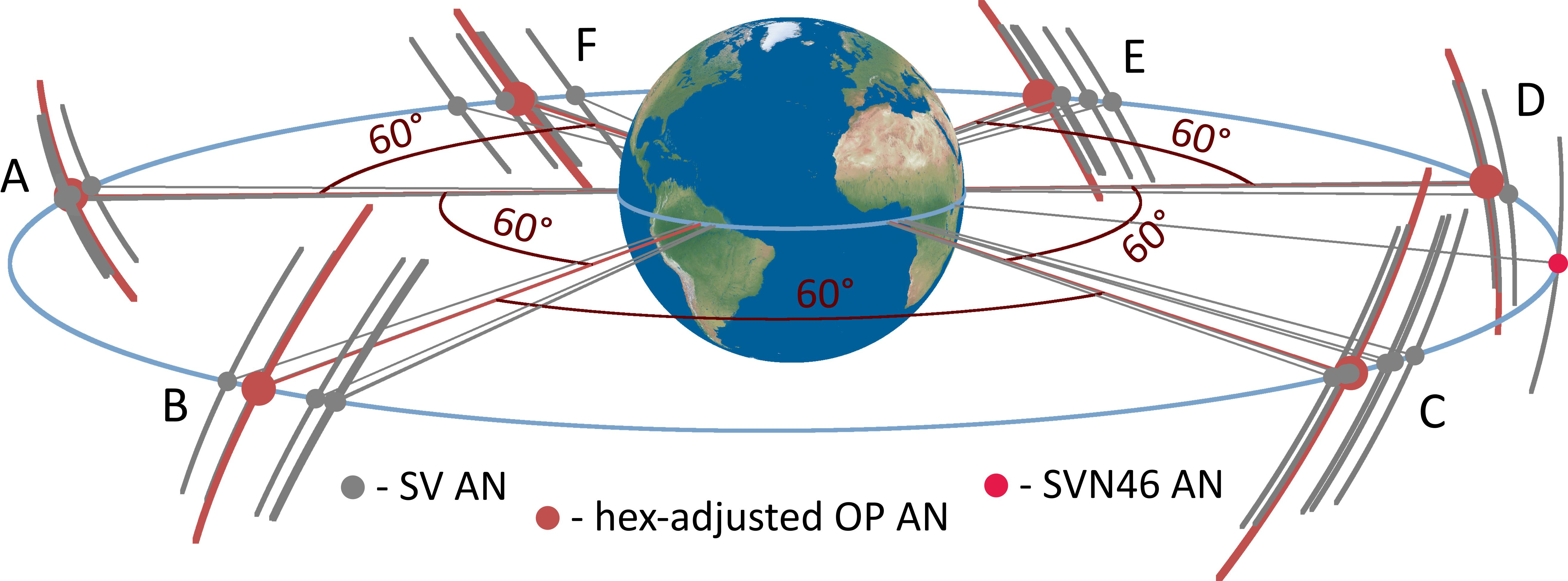
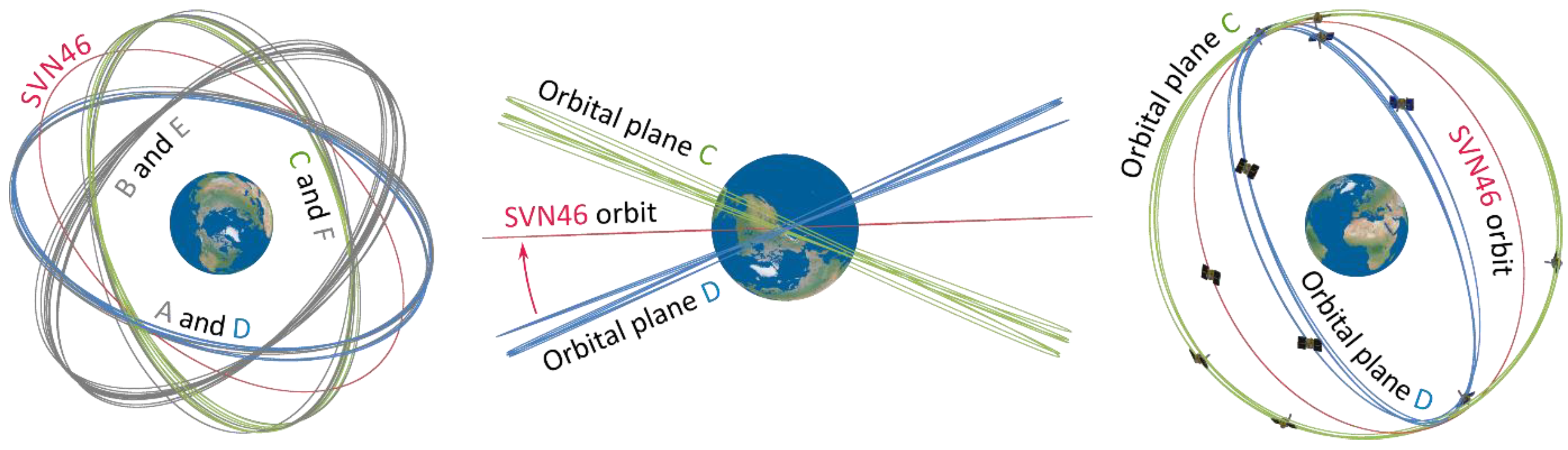
This work presents the spatial relationships of the GPS orbits, with emphasis on the symmetry of the ascending nodes. The study complements the current knowledge in the field of satellite geodesy with a broader perspective on the GPS constellation. In a previous study, Specht and Dabrowski [13] discussed the separation from the orbital plane D of the orbit of the Satellite Vehicle Number 46 (SVN46) transmitting the Pseudo-Random Noise 11 (PRN11) code. The authors indicated a systematic separation of the satellite orbit from the orbital plane. This long-term process resulted in an anomalous position relative to the GPS satellite constellation. Due to the limitations of the previous analysis, the present work was extended to all orbital planes and all almanacs available online. Excluding almanacs published before the 847th GPS week, the source data consisted of 7035 System Effectiveness Model (SEM) almanac files. The SEM almanacs contain Keplerian elements and other GPS satellites’ orbital parameters determined for a given epoch. The initial GPS constellation consisted of concept validation block I satellites launched into three 63° inclined orbital planes [14]. Hence, the comparative analysis based on the current constellation of six orbital planes with a 55° inclination used only satellites of block II and later. In the nominal form of the GPS space segment, the orbital planes are distributed symmetrically and separated by about 60° on the equator [15].
The satellite orbit parameters achieved for each launch are never perfect and deviate from nominal values within certain limits. For instance, SPS [16] informs that the achieved orbit inclination for any specific GPS satellite can be anywhere within 3° of the nominal inclination of 55°. The time derivative of the longitude of the ascending node (Ω) is a function of the achieved orbit inclination and orbit semi-major axis. As the GPS control segment does not remain passive due to changes in the constellation of satellites, some constellation tolerances and management practices need to be indicated. From time to time, orbit adjustments (thrusts) are performed to manage the constellation. Orbit maneuvers require a pause in the satellite mission as they cause discontinuities in the satellite track. The scheduled satellite outage times are provided by the control segment in the form of the Forecast Delta-V (FCSTDV) messages. The USCG [17] informs that, according to the maintenance procedure, the user may be required to download a new almanac. Further, FCSTDVs are not likely directly used to change the Ω of a given satellite. However, there may be some small unintentional change to Ω since other parameters such as the orbit’s semi-major axis may be slightly adjusted. The orbit separation of each satellite is presented at regular near-current epochs by the USCG [17] in the form of a slant chart. However, the diagram presents only temporary separation values and does not present a long-term process trend for both the satellites and the orbital planes.
This work was motivated by the presentation of the symmetry of the position of the ascending nodes of the six GPS orbital planes. In the first phase, the developed algorithm selected and assigned the satellites to individual orbital planes (OPs) based on the SEM almanac. The satellite longitude of the ascending node (Ω) parameter, due to perturbations and other external factors, took different values in the OP subsets. Determining the position of the ascending nodes of OPs required the use of estimation methods that take into account the presence of anomalies. In this, the position of the ascending nodes was determined using a robust estimation method [17,18] with the use of the Huber weight function [19]. In the next step, the algorithm compared the determined values of the six ascending nodes with the nominal symmetric distribution of nodes around the equator. The least-squares method was used to derive the estimators indicating the theoretical reference position of the OP ascending nodes. The use of the algorithm on the set of all 7035 almanacs resulted in the creation of datasets enabling the assessment of the ascending node (AN) separation trend. The limitation of the study is the use of broadcast almanac data rather than processed code and phase observations from worldwide stations. However, taking into account the mean several hundred-meter accuracy of the almanac parameters referred to precisely as Standard Product 3 data and the GPS orbit mean radius of 26,500 km, the impact of the error on Ω values is smaller than 0.003°.
The work is organized in the following sections: The second section presents the research methodology with a data processing algorithm. The third section contains the AN symmetry analysis results and general trend values for satellites in six OPs. The work ends with a summary containing the main conclusions of the study.
2. Materials and Methods
According to the ICD-GPS-240 interface [20], the GPS almanac is available in two formats: YUMA and System Effectiveness Model (SEM). The format name YUMA comes from the Yuma Proving Ground in Arizona (USA), where numerous tests on the GPS accuracy were performed. Apart from the differences in units and the number of parameters, the YUMA format is distinguished by the content of text descriptions. The SEM format has a tabular structure with greater variables precision than YUMA. For this reason, the SEM format was used in this work. The almanac files since 1997 are available on the United States Coast Guard website [21]. Previous almanacs (since 1991) can be obtained from The Center for Space Standards & Innovation website [22]. Due to the different initial orbit configurations, the analysis omitted the almanacs containing the parameters of the block I satellites. In the almanac generated in the 846th week and the 32,768th s of GPS time, SVN10 (PRN12) appears for the last time. The first almanac used in this study represents the epochs of the 847th week and the 61,440th s of GPS time on 24 March 1996. In total, 7035 SEM almanacs were used in this study. A total of 39 files were downloaded from the CSSI (years: 1996–1997) and 6996 files were downloaded from the USCG (years: 1997–2020). Until the year 2000, the GPS control segment published almanac files with a weekly frequency with several periods of longer breaks, e.g., in 1999. Currently, the almanacs are updated daily.
Two parameters in the GPS almanac parameters were used in the research: Ω and the rate of the longitude of the ascending node (dot(Ω)). The position of GPS orbit ANs in the almanac model is referenced to the Greenwich meridian at the beginning of the GPS week [23]. Therefore, in the description of the trajectory of satellites, Ω is used instead of the classic Keplerian right ascension of the ascending node related to the First Point of Aries. In astronomy, the position of stars and other celestial objects is defined in the equatorial coordinate system using angular coordinates. The coordinates are not fixed to the Earth but determined on the celestial sphere. The reference direction in the celestial equator plane is the First Point of Aries, also called the Vernal (March) Equinox. The GPS inertial system, based on the Greenwich meridian, defines the orientation of the coordinate axes with respect to the Earth, not the celestial sphere. To ensure the recurrence of Earth-centered Earth-fixed (ECEF) tracks of the GPS satellites, an additional force is applied to the satellites in the process of placing the satellite in the orbit. Its direction and magnitude compensate for the rotation of the Earth and result in the delay of the ANs’ drift. That additional angular velocity of the GPS satellites is expressed in the almanac by the dot(Ω) parameter. As the angular degrees were the unit used in the calculations, the conversion of the SEM almanacs’ semicircles was introduced.
To achieve the aim of the study, the algorithm with seven modules was developed (Figure 1). The first module selected the Ω and dot(Ω) values from the SEM almanacs. The second module of the algorithm assigned the satellites to the six GPS orbital planes. The third module used a robust estimation method to determine the position of the ascending nodes of the orbital planes based on the Ω parameter. The fourth module of the algorithm performed a least-squares method adjustment and determined the reference estimators satisfying the condition of the hexagonal symmetry of the ascending nodes of the orbital planes. The fifth module compared the positions of the ascending nodes of the individual satellites with the reference values of the orbital planes. After all the SEM almanacs had been processed, the last two steps of the calculation were run. The sixth module determined the satellite AN separation trend in relation to the OP based on the calculated values of deviations dΩ. The last, i.e., seventh, module of the algorithm determined the symmetry parameters of the adjusted OP ANs relative to the reference values.
The module 2 allocation procedure was applied using the position of the satellite orbit ANs indicated by the Ω parameter. Assuming the theoretical symmetrical 60-degree distribution of the GPS OPs in the equator plane, six satellite subsets, A, B, C, D, E, and F, with similar Ω parameter values were extracted. As an example, according to the last processed almanac from the 2123rd (75th in the current third cycle) GPS week and the 319,488th s (16 September 2020 16:44:48 UTC), the state of the constellation OPs was as follows: 4 (A), 5 (B), 5 (C), 6 (D), 6 (E), and 5 (F) satellite vehicles (SVs). In the set of all 31 almanacs’ Ω values, six subsets with the size of 4, 5, 5, 6, 6, and 5 elements were created with the GPS OPs’ satellites. In the 24-year-long research timeframe, the cardinality and elements of the OP subsets were changing due to space segment modernization. The six Ω-dependent subsets of satellites provided information on the spatial distribution of the orbit ANs in the equatorial plane.
As the almanacs do not contain information on the satellite OP designation, a method to assign the six subsets with OP alphabetical indicators was developed. Based on the Current Operational Advisories published on the USCG website, it was established that the SVN46 (PRN11) satellite has been carrying out its space mission continuously since 2000 and belongs to OP D. According to the prograde movement direction of the GPS satellites, the other OP subsets were assigned as A, B, C, E, and F for the almanacs generated between 2000 and 2019. For the remaining almanacs from 1996 to 2000, an analogous procedure was used based on the SVN18 (PRN18) satellite from orbital plane F. The application of algorithm module 2 resulted in the creation of six GPS OP subsets containing the parameters of the satellites for each SEM almanac file. The sample result of the application of module 2 of the algorithm is presented in Table 1.
The values of the Ω parameter in six subsets indicate the position of the satellite ANs at the almanac epoch. The subsets have a different degree of convergence of the satellite Ω parameter. Specht and Dabrowski [13] indicated the existence of a significant deviation in the position of the SVN46 (PRN11) satellite ascending node in relation to other OP D satellites (Figure 2).
The Earth-centered inertial (ECI) frame is a non-accelerating, non-rotating frame aligned with the Earth-centered Earth-fixed (ECEF) frame at a specific instant of time [24]. The presence of the indicated and potentially other outliers in OPs required applying a method that minimizes their impact on the estimators of the position of orbital plane ascending nodes. In this study, the robust estimation method [18] with the Huber damping function [19] was used. According to the M-estimation theory, it is a generalization of the maximum likelihood method consisting of the determination of M-estimators minimizing the objective function φ [25]:
where is an observation vector, is a vector of the determined parameters, is a function not necessarily resulting from the probabilistic properties of the variables, and is a vector of theoretical observational corrections. Assuming that the function is differentiable, the optimization criterion is solved by the equation:
Determining the gradient of the objective Function (1)
it can be written that the M-estimators are values that satisfy the following system of equations:
Expressions in formulas (3) and (4) can be equated as a proportional function to the influence function described by Hampel [26]. Due to the existing proportionality of the function and , the function is referred to as the influence function [17]. Based on the influence function, a specific form of the weight function is determined which plays a particularly important role in the robust estimation context:
In this least-squares method, with the objective function , the weight function takes the form , where is the matrix of weights created based on the assumed errors of the mean observations. In the study, an iterative calculation method was used, where the weight function in each repetition defined the modification of the original weights of observations . At each iteration step, a new observation weight was determined in relation to the absolute value of the estimator using the Huber weight function that eliminates the influence of gross errors on the estimation results [27]:
The variable t is interpreted as a control parameter with a significant impact on the length and efficiency of the iterative process. In the weight Function (6), the parameter t defines the acceptable range for standardized observational corrections . If the standardized correction is outside the range of acceptable values of measurement errors, then in the subsequent iteration steps, the weight of the i-th observation will be reduced to the value that eliminates the influence of the observation yi the final estimation results. The value of the parameter t is generally taken as 1.5, 2, 2.5, or 3.
Using the general form of the weight Function (6), Equation (4) can be written as
where is the diagonal matrix of the weight function. The solution to Equation (2) is the M-estimator of the parameter vector with the following form:
where j = 1, …, c is the number of iterative steps in the process of determining the M-estimator.
Formula (6) shows that the weight function values are modifications of the original observation weights from the least-squares method algorithm. Determined weight values were used as values initiating the iterative process of the robust M-estimators calculation. Moreover, the weight function of the i-th observation in the robust M-estimate can also be written using the damping function , where is the equivalent weight of the i-th observation in a given iteration step. Then, in the iterative process (8), there is an equivalent matrix of weights:
which is a modification of the weight function resulting from the application of the damping function of the Huber method:
The iterative process of determining the M-estimator (8) can be considered completed when in the c-th iteration step, the obtained M-estimator satisfies Equation (7) and the damping matrix is the identity matrix:
In practice, the standard deviation is unknown and is generally replaced by the error of the mean of the measured quantity. For this reason, also the standardization of corrections is carried out based on the determined errors of the mean corrections . The covariance matrix of the vector has the following form [17]:
where the diagonal elements of the matrix are the squares of the mean errors and is the estimator of the variance coefficient. The difference is the number of redundant observations calculated from the number of observation equations n and the number of parameters m.
The results of the robust estimation for the OP D subset are shown in Figure 3. The arithmetic mean of the satellites Ω is not a valid position estimate of OP ANs and is marked in black. This is due to a significant anomalous separation of the SVN46 orbit from the remaining OP D satellites. A significantly greater value of the correction in iteration (8) resulted in a reduction in the observation weight by the Huber damping Function (6) to the value minimizing the impact of observations on the final value of the OP D AN position estimator.
Due to the perturbations in the movement of GPS satellites and the modernization of the space segment occurring in the 24-year research timeframe, the position of six OP ANs did not meet the theoretical division of the full angle into six equal parts. The assessment of hexagonal symmetry required the calculation of reference values that met the condition of the angular separation between successive nodes amounting to 60°. The adjustment procedure is abbreviated here as hex-LS. Based on the robust estimators of the position of OP ANs determined in module 3 of the algorithm, observational equations of the angles between the ANs were created and then adjusted using the least-squares method. The design matrix defining the theoretical hexagonal geometry and the vector of intercepts y took the following forms:
where are the angles between the values of robust estimators determined in module 3 of the algorithm, e.g., . The weights of individual observations were set as equal due to the earlier application of the Huber function that minimized the impact of outliers. The weight matrix was a unit matrix, . The vector of corrections to the parameters was determined by adopting the optimization criterion of the least-squares method:
Estimators obtained from the hex-LS adjustment were the reference quantities for a given epoch of the SEM almanacs. Based on them, the dΩ deviations of the position of the satellite ANs relative to the OP were determined in algorithm module 5. Comparing the estimators of the robust method and the hex-LS method in module 7, the angular separations of OPs relative to the theoretical geometric conditions of the GPS were determined. The sample results of the estimation procedures from modules 3 and 4 are shown in Figure 4.
The figure shows the position of the OP ANs obtained at the consecutive stages of calculations. The arithmetic mean of the OPs’ Ω parameter is marked in black. The result of the robust method is shown in green. The final reference position of the OP ANs meeting the condition of hexagonal symmetry is marked in red. The ascending nodes of the orbits of individual GPS satellites are shown in gray with pink highlighting the anomalous orbit of the SVN46 satellite. The orthogonal view with a longitude of 90° N allows for a preliminary assessment of the correctness of the algorithm result on the example of the most characteristic OP, D. The perspective view shows fragments of the ECI orbits located near the ascending nodes.
Module 6 of the algorithm determined the trend of separation of the GPS satellite AN from the OP. The parameters of the regression lines were calculated using the least-squares method presented in Montgomery et al. [28]:
where is the regression line slope, is the regression line y-intercept, is the subset cardinality, is the satellite AN separation from the reference position of the OP, and is the almanac epoch converted from GPS time to years. Determined regression lines eliminated the impact of step changes in the dΩ parameter values caused, e.g., by GPS space segment modernization, resulting in a change in the number of satellites in OPs. The number of almanacs used provided large dΩ and dot(Ω) statistical sample datasets consisting of hundreds and thousands of elements. The cardinality of the samples allowed a reliable comparative analysis of orbit ANs of both active and inactive satellites operating between 1996 and 2020.
3. Results
The research algorithm consists of two basic levels. The first one processes data from a single SEM almanac and determines the epoch-specific descriptive parameters. To calculate the instantaneous angular separation dΩ of a particular GPS satellite, it is necessary to indicate a reference quantity. In the present study, a robust estimation method and the least-squares method with geometric conditions for the adjusted observations were used. The obtained results were saved to separate files grouped with respect to OPs and identified by the SVN and PRN identifiers of the satellites. Based on the time-tagged parameters of the satellites, the algorithm implemented second-level procedures using data from the research timeframe.
Due to the large amount of data processed, here are presented the results on one OP (D) standing out from the constellation. The interested reader will find detailed information on the other five OPs in the Appendix A. General conclusions about the GPS constellation are presented in the second part of this section. The analysis describes the satellite Ω parameter values and the OP ANs’ symmetry as a function of time. To improve the dΩ separation data interpretation, the angular unit used in the study is degrees converted from the SEM almanacs’ semicircles, and years converted from the GPS time notation are the time unit. The week was selected as the time unit for dot(Ω).
The results of the algorithm application are presented in Figure 5. The upper panel of the figure shows the values of dΩ separations from the two-stage estimated position of the OP D AN over the period 1996–2020. The lower panel shows the synchronous values of the dot(Ω) parameter of the satellites.
An anomaly in orbital motion in the set of GPS satellites was detected. The SVN46 satellite was launched in October 1999 and is still an active part of the space segment. The position of SVN46 AN is delayed relative to the remaining OP D satellites and is systematically closing to OP C (Figure 2). Additional confirmation of the unique separation trend of the SVN46 satellite orbit was found in a significantly smaller value of dot(Ω), which resulted in a slower shift of the orbit AN. While the remaining OP D satellites showed dΩ separation not exceeding several degrees in most cases, SVN46 obtained a change of 26.2° from an initial value of −1.2° in 2000 to −27.4° in 2020. The first and second week number rollovers’ vertical markers represent the midnights of 21–22 August 1999, and 6–7 April 2019, respectively. At the beginning of every 1024th GPS week, the week number in the navigation message is set to zero since only 10 bits are reserved for the week number [29].
Based on the time-tagged values of the dΩ parameter, the satellite AN separation trend from the OP was determined (Table 2). Each satellite in the list is described according to the current activity in the GPS space segment (SVA), satellite orbit AN separation rate from the OP (a), space mission duration (MD), number of SEM almanacs analyzed (n), and current dΩ value. The graphical interpretation of the dΩ trend in the research timeframe is shown in Figure 6.
The results of the analysis indicate that the magnitude of the satellite AN separation from the OP does not exceed, in seven out of ten cases, the absolute value of 0.3°/year. The remaining three satellites obtained values of −0.45° (SVN45), 0.40° (SVN75), and −1.34°/year (SVN46). Among the three largest trend values is the satellite of block IIIA (SVN75, PRN18), launched on 22 August 2019. Two obtained separation values represented only 29.9% (SVN75) and 33.6% (SVN45) of the absolute value of the AN separation rate compared to the third anomalous SVN46.
The comparison of the separation rate of all analyzed satellites is shown in Figure 7. The plot has two vertical scales. The scale on the left shows the rate of separation (SR) of the AN from the OP and refers to the left bars of the presented GPS satellites. Red and green bars represent inactive and active satellites, respectively. The blue bars on the right indicate the duration of the space mission (MD) described by the vertical scale on the right side of the plot. An additional element of the figure is information about the generations of individual GPS satellites expressed by circles in different colors placed above the SR and MD bars for different blocks.
A detailed interpretation of the chart is divided into three aspects presented in Table 3, Table 4 and Table 5. The first analysis shows the division of active and inactive satellites according to the absolute value of the satellite AN separation trend from the OP.
The number of active and inactive satellites in the applied ranges is similar. About 65% of the analyzed satellites achieved |a| values less than 0.3°/year with approximately 50% within the range of 0.1°–0.3°/year. The highest values exceeding 0.5°/year represent ca. 5% of the total population of satellites. The relationship between the duration of the satellite mission and the trend of separation is presented in Table 4.
The statistical sample was divided according to the duration of the satellite space mission. The difference in the percentages of the active and inactive GPS satellites is noticeable. Increases of 9.8% and 7.0% in the number of active satellites compared to the inactive in the 5–10 years and 10–15 years MD groups, respectively, occurred. A significant decrease in the number of active satellites amounting to 24.5% occurred in the range of 15–20 years. In the current GPS constellation, four out of all five satellites operate with a mission duration longer than 20 years. The corresponding mean absolute value of the OP AN separation trend equals 0.54°/year. However, in that case, a significant value of the standard deviation should be noted, caused by the anomalous and several times greater separation trend of the SVN46 satellite. The results show a general upward trend of |a| while the duration of the satellite space mission increases. However, this relationship is not close to linear, as the correlation coefficient of both parameters is 0.36. The third analysis of the separation trend based on the data in Figure 7 is shown in Table 5.
Excluding the block I satellites from the analyzed population, slightly larger numbers of satellites located on OPs B, E, and F than in the cases of the A, C, and D orbital planes are noticeable. Similarly to the previous analysis in Table 4, a significant impact of the PRN46 satellite with OP D on the mean value of |a| was noted. The highest absolute value of the separation of the AN from the OP is obtained in OP D and equals 0.37°/year. At the same time, the corresponding value of the standard deviation indicates the presence of smaller values of the remaining satellites from OP D. The other OPs’ |a| values range from 0.19° (OP F) to 0.26°/year (OP B). The values of their standard deviations indicate a similar separation rate of the remaining OP satellites. The average satellite mission durations range from 10.59 to 12.86 years. The longest mean MD was recorded for OP A and OP D.
The study showed a stepwise but systematic increase in the standard deviation of dΩ separations in the case of all six OPs (Figure 8). OP D stands out with a 5-fold increase in the last 24 years from a value not exceeding 2° in 1996 to 10° in 2020. The impact of the anomalous position of SVN46’s orbit is apparent. The A, B, E, and F OPs’ dΩ standard deviations ranged from 2° to 3°. An approximately 1° higher value occurred in OP C at the end of the analysis in 2020. A major decrease in the OP C dΩ standard deviation was observed in 2015 when the SVN33 and SVN36 satellites ended their mission. The satellites’ dΩ values at the end of their activity equaled −10.37° and −5.09°, respectively. Significantly larger separations of their ANs resulted in high values of the standard deviation of OPs.
The step changes in the standard deviations were caused by the modernization of the GPS space segment and the change in the number of active satellites. Confirmation of this relationship is indicated by the last chart’s parameter presenting the number of active OP D satellites. Comparing the epochs of the change in the number of satellites (black) with the corresponding dΩ standard deviation (green), a coincidence is visible. In general, the step changes did not change the upward trend of the standard deviations of the GPS satellites’ AN separations from the OP.
The last point of the study was the analysis of the adjusted OP Ω values. Figure 9 shows the derived estimators of the OP ANs’ symmetry. In the left part of the figure, the red vertical arrows indicate the hexagonal symmetry between the six OPs of the GPS space segment. The orbital planes A, B, C, D, E, and F are presented from bottom to top in the figure. The horizontal red lines refer to the reference values of the research, i.e., hex-LS adjustment results providing the initial GPS geometry with the hexagonal division of the equatorial plane by OPs. Using the hex-LS estimators, the robust adjustment Ω deviations (green color) were calculated. The last elements of the figure are marked in black: deviations of the OPs arithmetic mean Ω values from the hex-LS reference. The colors of the parameters correspond to Figure 3 and Figure 4.
The dΩ OP D deviation values took the smallest and the largest values in the dataset from −7° to 3.5°. In the case of the remaining OPs, the deviations mostly range from −2° to 2°. The differences in the course of the polylines representing the arithmetic mean (black) and the robust estimation (green) method indicate minimization of the impact of outliers on the determined OP AN position robust estimator. The results are visible, e.g., in the case of OP D, where almost from the beginning of the SVN46 mission in 2000, the weights of its anomalous orbit were systematically minimized. In the research timeframe, for all OPs except for OP D, similar values of approximately 2° of the AN position error with respect to the hex-LS estimators were obtained. This OP AN deviation doubled in OP D in 2012 and has tripled since 2018. In the last two years, the OP AN deviations remained relatively constant in five out of six OPs. The exception is OP F, where a reverse trend of the OP AN closing to the initial symmetry was noted.
4. Conclusions
This work presents a novel method of assessing the symmetry of the ascending nodes of the GPS orbital planes. Previous space segment studies focused mainly on the accuracy of determining the position of satellites. This study provides a more general perspective and is an extension of the conclusions drawn from the previous authors’ research on the anomalous orbit of one of the GPS satellites. The research material consisted of 7035 SEM almanacs containing crucial Keplerian orbital parameters and published between 1996 and 2020. Based on the longitude of the ascending node (Ω) and rate of the longitude of the ascending node (dot(Ω)) parameters, the symmetry properties of the satellite orbits’ ascending nodes were determined.
The research algorithm included robust estimation and least-squares adjustment methods. The reference values estimated for each almanac epoch met the requirement of the initial GPS hexagonal symmetry of orbital plane ascending nodes in the equatorial plane. The estimators were determined in two stages. In the first stage, the Huber weight function eliminated the influence of outliers in the ascending node Ω datasets. The second stage introduced the condition of hexagonal symmetry in the least-squares method. The reference Ω values of the orbital plane ascending nodes were used to determine the dΩ deviations and the separation trend values of the ascending nodes of individual GPS satellites. The symmetry of the GPS orbital planes was also analyzed.
The study showed that for five out of six orbital planes, the hexagonal ascending nodes symmetry error value did not exceed 2°. An exception was orbital plane D, where three times higher values of deviations were recorded. In this case, the robust estimation method was of particular importance as it minimized the impact of the anomalous SVN46 satellite orbit on the adjustment results. The analysis showed an average trend of separation of satellite ascending nodes from the orbital planes of 0.25°/year with an average space mission duration of 11.7 years. The highest value of the separation trend was obtained for orbital plane D with the anomalous SVN46. The study also assessed the impact of the space mission duration on the ascending node separation trends. With a correlation coefficient of 0.36, the highest mean trend value of 0.54°/year occurred in the case of satellites operating for over 20 years. Satellites with less than 5 years of mission duration achieved four times lower values.
The developed method for assessing the symmetry of the position of the orbital plane ascending nodes is a novel solution to obtaining information about the current and past states of the satellite constellation. Adaptation of thousands of GPS almanacs to a statistical sample increased the reliability of the analysis. The trend of satellite ascending node separation from orbital planes determined in the 24-year-long research timeframe additionally enables the prediction of the future constellation state and can significantly support the actions of the GPS control segment.
Funding
This research was funded from the statutory activities of Gdynia Maritime University, grant number WN/2020/PZ/05.
Institutional Review Board Statement
Not applicable.
Informed Consent Statement
Not applicable.
Data Availability Statement
Publicly available datasets were analyzed in this study. This data can be found here: https://www.navcen.uscg.gov, and https://celestrak.com.
Conflicts of Interest
The author declares no conflict of interest.
Appendix A

Table A1.
Descriptive parameters of the OP A satellites.
| SVN | PRN | OP | SVA | a [°/Year] | MD [Year] | n | dΩ [°] |
|---|---|---|---|---|---|---|---|
| 19 | 19 | A | NO | −0.44 | 5.45 | 598 | - |
| 25 | 25 | A | NO | −0.3 | 13.72 | 3114 | - |
| 27 | 27 | A | NO | −0.15 | 16.52 | 4026 | - |
| 38 | 8 | A | NO | 0.26 | 17.36 | 4788 | - |
| 39 | 9 | A | NO | −0.06 | 18.14 | 4735 | - |
| 48 | 7 | A | YES | 0.11 | 12.49 | 4532 | 0.84 |
| 52 | 31 | A | YES | 0.17 | 13.95 | 5053 | 1.64 |
| 64 | 30 | A | YES | −0.23 | 6.56 | 2386 | 1.97 |
| 65 | 24 | A | YES | −0.26 | 7.94 | 2886 | −3.43 |
Figure A1.
Separation of satellite ANs from the hex-LS-estimated position of the OP A AN with satellite dot(Ω) values.
Figure A1.
Separation of satellite ANs from the hex-LS-estimated position of the OP A AN with satellite dot(Ω) values.

Table A2.
Descriptive parameters of the OP B satellites.
| SVN | PRN | OP | SVA | a [°/Year] | MD [Year] | n | dΩ [°] |
|---|---|---|---|---|---|---|---|
| 13 | 2 | B | NO | −0.39 | 8.12 | 1241 | - |
| 20 | 20 | B | NO | −0.13 | 0.69 | 33 | - |
| 22 | 22 | B | NO | −0.4 | 7.35 | 1054 | - |
| 30 | 30 | B | NO | −0.22 | 14.8 | 3689 | - |
| 35 | 05, 30 | B | NO | −0.35 | 17.09 | 3492 | - |
| 44 | 28 | B | YES | 0.25 | 20.06 | 6615 | 4.6 |
| 49 | 1 | B | NO | −0.06 | 1.14 | 414 | - |
| 56 | 16 | B | YES | 0.29 | 17.61 | 6101 | 4.53 |
| 58 | 12 | B | YES | 0.34 | 13.81 | 5002 | 3.72 |
| 62 | 25 | B | YES | 0.2 | 10.32 | 3745 | 0.14 |
| 71 | 26 | B | YES | −0.23 | 5.47 | 1991 | −2.03 |
Figure A2.
Separation of satellite ANs from the hex-LS-estimated position of the OP B AN with satellite dot(Ω) values.
Figure A2.
Separation of satellite ANs from the hex-LS-estimated position of the OP B AN with satellite dot(Ω) values.

Table A3.
Descriptive parameters of the OP C satellites.
| SVN | PRN | OP | SVA | a [°/Year] | MD [Year] | n | dΩ [°] |
|---|---|---|---|---|---|---|---|
| 28 | 28 | C | NO | 0.15 | 1.38 | 123 | - |
| 31 | 31 | C | NO | −0.29 | 9.57 | 1644 | - |
| 33 | 3 | C | NO | −0.57 | 18.32 | 4810 | - |
| 36 | 6 | C | NO | −0.4 | 17.9 | 4649 | - |
| 37 | 7 | C | NO | −0.29 | 11.73 | 2421 | - |
| 53 | 17 | C | YES | 0.19 | 14.96 | 5416 | 2.82 |
| 57 | 29 | C | YES | 0.24 | 12.72 | 4613 | 3.59 |
| 59 | 19 | C | YES | 0.13 | 16.47 | 5829 | 5.34 |
| 66 | 27 | C | YES | 0.2 | 7.33 | 2663 | −0.12 |
| 72 | 8 | C | YES | −0.02 | 5.16 | 1880 | −1.08 |
Figure A3.
Separation of satellite ANs from the hex-LS-estimated position of the OP C AN with satellite dot(Ω) values.
Figure A3.
Separation of satellite ANs from the hex-LS-estimated position of the OP C AN with satellite dot(Ω) values.

Table A4.
Descriptive parameters of the OP E satellites.
| SVN | PRN | OP | SVA | a [°/Year] | MD [Year] | n | dΩ [°] |
|---|---|---|---|---|---|---|---|
| 14 | 14 | E | NO | 0.22 | 4.04 | 402 | - |
| 16 | 16 | E | NO | 0.18 | 4.51 | 427 | - |
| 21 | 21 | E | NO | 0.18 | 6.83 | 928 | - |
| 23 | 23, 32 | E | NO | 0.06 | 19.83 | 4277 | - |
| 40 | 10 | E | NO | −0.05 | 18.93 | 5136 | - |
| 47 | 22 | E | YES | −0.57 | 16.72 | 5888 | −5.08 |
| 50 | 5 | E | YES | −0.1 | 11.07 | 4017 | −1.88 |
| 51 | 20 | E | YES | −0.47 | 20.29 | 6627 | −7.55 |
| 54 | 18 | E | NO | −0.46 | 17.05 | 5647 | - |
| 69 | 3 | E | YES | 0.18 | 5.87 | 2136 | 0.04 |
| 73 | 10 | E | YES | 0.11 | 4.86 | 1770 | −0.26 |
| 76 | 23 | E | YES | −0.02 | 0.18 | 67 | −1.64 |
Figure A4.
Separation of satellite ANs from the hex-LS-estimated position of the OP E AN with satellite dot(Ω) values.
Figure A4.
Separation of satellite ANs from the hex-LS-estimated position of the OP E AN with satellite dot(Ω) values.

Table A5.
Descriptive parameters of the OP F satellites.
| SVN | PRN | OP | SVA | a [°/Year] | MD [Year] | n | dΩ [°] |
|---|---|---|---|---|---|---|---|
| 18 | 18 | F | NO | −0.15 | 4.38 | 420 | - |
| 26 | 26 | F | NO | 0.28 | 18.77 | 4966 | - |
| 29 | 29 | F | NO | 0.14 | 11.57 | 2363 | - |
| 32 | 1 | F | NO | 0.17 | 11.97 | 2502 | - |
| 41 | 14 | F | NO | 0.25 | 19.55 | 6532 | - |
| 43 | 13 | F | YES | 0.37 | 23.11 | 6908 | 7.24 |
| 55 | 15 | F | YES | −0.44 | 12.89 | 4671 | −6.14 |
| 60 | 23 | F | NO | −0.11 | 15.7 | 5576 | - |
| 68 | 9 | F | YES | 0.05 | 6.12 | 2224 | −0.97 |
| 70 | 32 | F | YES | 0.06 | 4.6 | 1675 | −0.62 |
| 74 | 4 | F | YES | −0.07 | 0.93 | 337 | 1.49 |
Figure A5.
Separation of satellite ANs from the hex-LS-estimated position of the OP F AN with satellite dot(Ω) values.
Figure A5.
Separation of satellite ANs from the hex-LS-estimated position of the OP F AN with satellite dot(Ω) values.

References
- Montenbruck, O.; Steigenberger, P.; Prange, L.; Deng, Z.; Zhao, Q.; Perosanz, F.; Romero, I.; Noll, C.; Stürze, A.; Schmid, R.; et al. The Multi-GNSS Experiment (MGEX) of the International GNSS Service (IGS)–achievements, prospects and challenges. Adv. Space Res. 2017, 59, 1671–1697. [Google Scholar] [CrossRef]
- Steigenberger, P.; Montenbruck, O. Galileo status: Orbits, clocks, and positioning. GPS Solut. 2017, 21, 319–331. [Google Scholar] [CrossRef]
- Gunning, K.; Walter, T.; Enge, P. Characterization of GLONASS broadcast clock and ephemeris: Nominal performance and fault trends for ARAIM. In Proceedings of the ION ITM, Institute of Navigation, Monterey, CA, USA, 30 January–2 February 2017; pp. 170–183. [Google Scholar]
- Ouyang, C.; Shi, J.; Shen, Y.; Li, L. Six-Year BDS-2 Broadcast Navigation Message Analysis from 2013 to 2018: Availability, Anomaly, and SIS UREs Assessment. Sensors 2019, 19, 2767. [Google Scholar] [CrossRef] [PubMed] [Green Version]
- Kim, M.; Kim, J. A long-term analysis of the GPS broadcast orbit and clock error variations. Procedia Eng. 2015, 99, 654–658. [Google Scholar] [CrossRef] [Green Version]
- Wang, H.; Jiang, H.; Ou, J.; Sun, B.; Zhong, S.; Song, M.; Guo, A. Anomaly analysis of 18 years of newly merged GPS ephemeris from four IGS data centers. GPS Solut. 2018, 22, 124. [Google Scholar] [CrossRef]
- Montenbruck, O.; Steigenberger, P.; Hauschild, A. Broadcast versus Precise Ephemerides: A Multi-GNSS Perspective. GPS Solut. 2015, 19, 321–333. [Google Scholar] [CrossRef]
- Sarkar, S.; Bose, A. Lifetime performances of modernized GLONASS satellites: A review. Artif. Sat. 2017, 52, 85–97. [Google Scholar] [CrossRef]
- Gunning, K.; Walter, T.; Enge, P. Multi-GNSS Constellation Anomaly Detection and Performance Monitoring. In Proceedings of the ION ITM, Institute of Navigation, Portland, OR, USA, 25–29 September 2017; pp. 1051–1062. [Google Scholar]
- Dai, X.; Ge, M.; Lou, Y.; Shi, C.; Wickert, J.; Schuh, H. Estimating the yaw-attitude of BDS IGSO and MEO satellites. J. Geod. 2015, 89, 1005–1018. [Google Scholar] [CrossRef]
- Ma, L.; Zhou, S. Positional accuracy of GPS satellite almanac. Artif. Sat. 2014, 49, 225–231. [Google Scholar] [CrossRef] [Green Version]
- Reid, T.G.; Walter, T.; Enge, P.K.; Sakai, T. Orbital representations for the next generation of satellite-based augmentation systems. GPS Solut. 2016, 20, 737–750. [Google Scholar] [CrossRef]
- Specht, C.; Dabrowski, P. Runaway PRN11 GPS satellite. In Proceedings of the 10th International Conference Environmental Engineering, Vilnius, Lithuania, 27–28 April 2017. [Google Scholar]
- Leick, A.; Rapoport, L.; Tatarnikov, D. GPS Satellite Surveying; John Wiley & Sons: Hoboken, NJ, USA, 2015. [Google Scholar]
- Teunissen, P.J.; Kleusberg, A. (Eds.) GPS for Geodesy; Springer Science & Business Media: Berlin/Heidelberg, Germany, 2012. [Google Scholar]
- SPS. Global Positioning System Standard Positioning Service Performance Standard. 2008. Available online: https://www.gps.gov/technical/ps/2008-SPS-performance-standard.pdf (accessed on 5 November 2019).
- Wiśniewski, Z. M-estimation with probabilistic models of geodetic observations. J. Geod. 2014, 88, 941–957. [Google Scholar] [CrossRef] [Green Version]
- Zienkiewicz, M.H. Application of M split estimation to determine control points displacements in networks with unstable reference system. Surv. Rev. 2015, 47, 174–180. [Google Scholar] [CrossRef]
- Huber, P.J. Robust estimation of a location parameter. In Breakthroughs in Statistics; Springer: New York, NY, USA, 1992; pp. 492–518. [Google Scholar] [CrossRef]
- ICD-GPS-240. Interface Control Document–Navstar GPS Space Segment/Navigation User Interfaces (ICD-GPS-240), Revision C. 2019. Available online: https://www.gps.gov/technical/icwg/ICD-GPS-240C.pdf (accessed on 1 September 2020).
- NAVCEN. U.S. Coast Guard Navigation Center. 2020. Available online: https://www.navcen.uscg.gov (accessed on 1 September 2020).
- CSSI. The Center for Space Standards & Innovation. Available online: https://celestrak.com (accessed on 1 September 2020).
- Montenbruck, O.; Gill, E. Satellite Orbits: Models, Methods and Applications; Springer: Berlin, Germany, 2012. [Google Scholar]
- Teunissen, P.; Montenbruck, O. (Eds.) Springer Handbook of Global Navigation Satellite Systems; Springer: Berlin/Heidelberg, Germany, 2017. [Google Scholar]
- Wiśniewski, Z.; Zienkiewicz, M.H. Shift-M split* estimation in deformation analyses. J. Surv. Eng. 2016, 142, 04016015. [Google Scholar] [CrossRef]
- Hampel, F.R. The influence curve and its role in robust estimation. J. Am. Stat. Assoc. 1974, 69, 383–393. [Google Scholar] [CrossRef]
- Ge, Y.; Yuan, Y.; Jia, N. More efficient methods among commonly used robust estimation methods for GPS coordinate transformation. Surv. Rev. 2013, 45, 229–234. [Google Scholar] [CrossRef]
- Montgomery, D.C.; Peck, E.A.; Vining, G.G. Introduction to Linear Regression Analysis; John Wiley & Sons: Hoboken, NJ, USA, 2012. [Google Scholar]
- Hofmann-Wellenhof, B.; Lichtenegger, H.; Wasle, E. GNSS-Global Navigation Satellite Systems. GPS, GLONASS, Galileo and More; Springer: Berlin/Heidelberg, Germany, 2008. [Google Scholar]
Figure 1.
The workflow of the research algorithm.

Figure 2.
Orbits of GPS satellites in the Earth-centered inertial (ECI) reference frame for the epoch 13 September 2020, 12:41:54 UTC.
Figure 2.
Orbits of GPS satellites in the Earth-centered inertial (ECI) reference frame for the epoch 13 September 2020, 12:41:54 UTC.

Figure 3.
Comparison of the determination of the orbital plane (OP) D ascending node (AN) using the arithmetic mean and the robust estimation method with the weight values of the observations.
Figure 3.
Comparison of the determination of the orbital plane (OP) D ascending node (AN) using the arithmetic mean and the robust estimation method with the weight values of the observations.

Figure 4.
Position estimators of OP ANs determined by the robust estimation method and hex-LS on 13 September 2020 in top (a), and perspective view (b).
Figure 4.
Position estimators of OP ANs determined by the robust estimation method and hex-LS on 13 September 2020 in top (a), and perspective view (b).

Figure 5.
Separation of satellite ANs from the hex-LS-estimated position of the OP D AN with satellite dot(Ω) values.
Figure 5.
Separation of satellite ANs from the hex-LS-estimated position of the OP D AN with satellite dot(Ω) values.

Figure 6.
The trend of separation of satellite ANs from OP D.

Figure 7.
Separation rate (SR) and space mission duration (MD) of GPS satellites.

Figure 8.
Standard deviations of the OPs’ dΩ parameter.

Figure 9.
Deviations of OP AN position estimators in relation to the hexagonal symmetry reference.

Table 1.
The assignment of satellites to orbital planes on the example of the GPS time third cycle almanac from epoch 75.319488.
Table 1.
The assignment of satellites to orbital planes on the example of the GPS time third cycle almanac from epoch 75.319488.
| OP | Ω [°] (SVN) | Mean Ω [°] | StDev Ω [°] |
|---|---|---|---|
| A | 241.4338 (48), 237.1903 (65), 242.6358 (64), 242.3521 (52) | 240.9030 | 2.1891 |
| B | 304.9308 (58), 306.0106 (56), 300.9003 (62), 298.7580 (71), 306.2207 (44) | 303.3641 | 2.9968 |
| C | 359.9438 (72), 4.1978 (53), 6.8009 (59), 0.8136 (66), 4.8822 (57) | 3.3277 | 2.5694 |
| D | 61.2960 (63), 56.7924 (61), 60.8234 (67), 33.6900 (46), 62.1870 (75), 56.8857 (45) | 55.2791 | 9.8795 |
| E | 120.8952 (69), 118.9797 (50), 120.7238 (73), 113.012 (51), 115.7114 (47), 119.4557 (76) | 118.1296 | 2.8547 |
| F | 182.7315 (74), 179.9369 (68), 188.2194 (43), 174.6445 (55), 180.4468 (70) | 181.1958 | 4.3990 |
Table 2.
Descriptive parameters of the OP D satellites.
| SVN | PRN | OP | SVA | a [°/Year] | MD [Year] | n | dΩ [°] |
|---|---|---|---|---|---|---|---|
| 15 | 15 | D | NO | 0.18 | 10.64 | 2029 | - |
| 17 | 17 | D | NO | 0.29 | 8.91 | 1427 | - |
| 24 | 24 | D | NO | 0.06 | 15.6 | 3720 | - |
| 34 | 04, 18 | D | NO | −0.25 | 23.53 | 5845 | - |
| 45 | 21 | D | YES | −0.45 | 17.44 | 6059 | −4.3 |
| 46 | 11 | D | YES | −1.34 | 20.69 | 6648 | −27.65 |
| 61 | 2 | D | YES | −0.3 | 15.84 | 5668 | −4.34 |
| 63 | 1 | D | YES | 0.2 | 9.15 | 3320 | 0.4 |
| 67 | 6 | D | YES | 0.2 | 6.32 | 2299 | −0.07 |
| 75 | 18 | D | YES | 0.4 | 0.51 | 187 | 1.12 |
Table 3.
Absolute values of the GPS satellite separation trends.
| |a| [°/Year] | Active SVs | Inactive SVs | SVs | |||
|---|---|---|---|---|---|---|
| <0.1 | 5 | 16.1% | 5 | 15.6% | 10 | 15.9% |
| 0.1–0.2 | 7 | 22.6% | 10 | 31.3% | 17 | 27.0% |
| 0.2–0.3 | 10 | 32.3% | 9 | 28.1% | 19 | 30.2% |
| 0.3–0.4 | 3 | 9.7% | 3 | 9.4% | 6 | 9.5% |
| 0.4–0.5 | 4 | 12.9% | 4 | 12.5% | 8 | 12.7% |
| >0.5 | 2 | 6.5% | 1 | 3.1% | 3 | 4.8% |
| Total: | 31 | 32 | 63 | |||
Table 4.
Mission duration (MD) and absolute value of the separation trend.
| MD [years] | Active SVs | Inactive SVs | SVs | |a| [°/Year] | ||||
|---|---|---|---|---|---|---|---|---|
| Mean | StDev | |||||||
| <5 | 5 | 16.1% | 6 | 18.8% | 11 | 17.5% | 0.14 | 0.10 |
| 5–10 | 9 | 29.0% | 6 | 18.8% | 15 | 23.8% | 0.24 | 0.11 |
| 10–15 | 8 | 25.8% | 6 | 18.8% | 14 | 22.2% | 0.22 | 0.09 |
| 15–20 | 5 | 16.1% | 13 | 40.6% | 18 | 28.6% | 0.27 | 0.17 |
| >20 | 4 | 12.9% | 1 | 3.1% | 5 | 7.9% | 0.54 | 0.41 |
| Total: | 31 | 32 | 63 | |||||
Table 5.
Absolute value of the separation trend and mission duration (MD) of GPS satellites in OPs.
| OP | Active SVs | Inactive SVs | SVs | |a| [°/Year] | MD [Years] | |||||
|---|---|---|---|---|---|---|---|---|---|---|
| Mean | StDev | Mean | StDev | |||||||
| A | 4 | 12.9% | 5 | 15.6% | 9 | 14.3% | 0.22 | 0.11 | 12.46 | 4.48 |
| B | 5 | 16.1% | 6 | 18.8% | 11 | 17.5% | 0.26 | 0.10 | 10.59 | 6.32 |
| C | 5 | 16.1% | 5 | 15.6% | 10 | 15.9% | 0.25 | 0.15 | 11.55 | 5.38 |
| D | 6 | 19.4% | 4 | 12.5% | 10 | 15.9% | 0.37 | 0.34 | 12.86 | 6.65 |
| E | 6 | 19.4% | 6 | 18.8% | 12 | 19.0% | 0.22 | 0.18 | 10.85 | 6.98 |
| F | 5 | 16.1% | 6 | 18.8% | 11 | 17.5% | 0.19 | 0.12 | 11.78 | 6.81 |
| Total: | 31 | 32 | 63 | |||||||
Publisher’s Note: MDPI stays neutral with regard to jurisdictional claims in published maps and institutional affiliations. |
© 2021 by the author. Licensee MDPI, Basel, Switzerland. This article is an open access article distributed under the terms and conditions of the Creative Commons Attribution (CC BY) license (http://creativecommons.org/licenses/by/4.0/).
Share and Cite
MDPI and ACS Style
Dabrowski, P.S. The Symmetry of GPS Orbit Ascending Nodes. Remote Sens. 2021, 13, 387. https://doi.org/10.3390/rs13030387
AMA Style
Dabrowski PS. The Symmetry of GPS Orbit Ascending Nodes. Remote Sensing. 2021; 13(3):387. https://doi.org/10.3390/rs13030387
Chicago/Turabian StyleDabrowski, Pawel S. 2021. "The Symmetry of GPS Orbit Ascending Nodes" Remote Sensing 13, no. 3: 387. https://doi.org/10.3390/rs13030387
Note that from the first issue of 2016, this journal uses article numbers instead of page numbers. See further details here.