Sea-Level Change along the Emilia-Romagna Coast from Tide Gauge and Satellite Altimetry


1
Department of Biological, Geological and Environmental Sciences, University of Bologna, 40126 Bologna, Italy
2
Istituto Nazionale di Geofisica e Vulcanologia, Sezione di Bologna, 40128 Bologna, Italy
*
Author to whom correspondence should be addressed.
Remote Sens. 2021, 13(1), 97; https://doi.org/10.3390/rs13010097
Submission received: 26 November 2020
/
Revised: 25 December 2020
/
Accepted: 25 December 2020
/
Published: 30 December 2020
(This article belongs to the Special Issue New Challenges in Sea Level Rise Observation)
Abstract
:Coastal flooding and retreat are markedly enhanced by sea-level rise. Thus, it is crucial to determine the sea-level variation at the local scale to support coastal hazard assessment and related management policies. In this work we focus on sea-level change along the Emilia-Romagna coast, a highly urbanized, 130 km-long belt facing the northern Adriatic Sea, by analyzing data from three tide gauges (with data records in the last 25–10 years) and related closest grid points from CMEMS monthly gridded satellite altimetry. The results reveal that the rate of sea-level rise observed by altimetry is coherent along the coast (2.8 ± 0.5 mm/year) for the period 1993–2019 and that a negative acceleration of −0.3 ± 0.1 mm/year is present, in contrast with the global scale. Rates resulting from tide gauge time series analysis diverge from these values mainly as a consequence of a large and heterogeneous rate of subsidence in the region. Over the common timespan, altimetry and tide gauge data show very high correlation, although their comparison suffers from the short overlapping period between the two data sets. Nevertheless, their combined use allows assessment of the recent (last 25 years) sea-level change along the Emilia-Romagna coast and to discuss the role of different interacting processes in the determination of the local sea level.
1. Introduction
Sea level lies among the 54 Essential Climate Variables (ECVs) that represent the Earth system’s key parameters, as defined and periodically assessed by the Global Climate Observing System (GCOS), in support of the United Nations Framework Convention on Climate Change (UNFCCC) and of the Intergovernmental Panel on Climate Change (IPCC). Direct observation of the sea level dates back to the 18th century [1] and this made possible realistic models for the sea-level variation and its interconnection with climate change. The ongoing sea-level change is the product of a continuous, mutable, and complex interaction among several components through the whole Earth system, combining natural and anthropic causes. It is commonly recognized that the increase in anthropogenic greenhouse gasses emission in the atmosphere, plus a small increment of natural solar irradiance, has led to a progressive effective radiative forcing (ERF) growth since the 1970s [2], hence to climate warming. More than 90% of the heat increase in the climate system, derived from the ERF, has been stored by the ocean, with the consequential thermal expansion and sea-level rise. At global scale, there is a general consensus that sea level has been rising at 1.7 ± 0.2 mm/year over the last century [2], and at 3.3 ± 0.5 mm/year over the last 25 years [3]. This is not a steady process since at both temporal scales, a positive acceleration (0.084 ± 0.025 mm/year2) was also confirmed [4,5]. Presently, there is the virtual certainty that sea-level rise and climate change will bring to society and the environment significant consequences, especially in low-elevation coastal zones where more than 620 million people live presently, a number that is expected to double by 2060 [6,7]. This enhances the climate-related concern about the sea-level rise impact at global scale and at coasts.
Satellite radar altimetry (SA) missions started in the early 1990s with the goal of providing, among other data, a fortnightly measure for the global sea surface height (SSH) in the reference system of the Earth’s mass center. Given its reference frame, this is commonly referred to as the absolute sea level (ASL). SSH represents the difference between the satellite altitude above the reference ellipsoid and the height of the satellite above the instantaneous sea surface, measured by transmitting microwave radiations toward the surface which are partly reflected to the satellite [8]. As a consequence of this configuration, SSH measurements are affected by several sources of uncertainties. Such uncertainties are resolved by compensating for the effect of instrumental drift, signal refraction passing through the atmosphere, Glacial Isostatic Adjustment (GIA), tides and atmospheric pressure influence whose correction is commonly known as the Dynamic Atmospheric Correction (DAC). However, in shallow water and at the coast SA data are influenced and contaminated by both the presence of land in the satellite footprint and the spatio-temporal scale reduction of atmospheric and oceanographic processes with respect to the open ocean [8,9,10]. The need for reliable coastal altimetry data has led over recent years to the development of new sophisticated altimetry products, where the improved reprocessing and dedicated corrections aim to extend valid measurement to within < 20 km from the coast [11,12,13].
On the contrary, tide gauges (TGs) provide a measure of the sea level with respect to the pier at which the TG is attached and for this reason it is commonly referred to as relative sea level (RSL). The largest TG database is the Permanent Service for Mean Sea Level (PSMSL), where almost two thousand TG time series are collected, periodically updated, and reduced to a common datum, producing the Revised Local Reference (RLR) dataset [14,15,16]. Developed for different purposes, i.e., the observation of the harbor tide, currently TG data used for long-term sea-level studies suffer from the contamination by the vertical land movement (VLM) of the pier itself. This problem was sorted out in the recent past by the co-location of GNSS (Global Navigation Satellite System) at the TG site. However, this practice only started since the late 1990s [17,18] and for this reason it does not cover the whole time series at most of the TG sites. Despite the long period coverage (since 19th century for some specific cases) TGs data are geographically limited because of their heterogeneous spatial distribution. TGs measurement has increased since the 1950s, primarily throughout the Northern Hemisphere [19]. This limitation generates a bias that may hinder accurate and reliable sea level consideration at global scale.
Despite SA and TG time series currently represent the two main source of information for the sea level, the contrast between their observational ability remains an unresolved point. RSL, measured by the TGs, reflects the local variations in sea level and it is influenced by the VLM effect and the coastal processes, differently from the SA ASL records that provide geocentric sea-level variations. SA and TG data sets are, moreover, characterized by low and high acquisition rate, respectively [11]. Only SA measurement allows observation of the variability on sea level from the open ocean towards the coastal area and it is considered essential for giving perspective at regional and global scale without resolving, however, some key coastal processes, which instead are recorded by TGs. RSL and ASL variation and VLM are linked by means of the Sea Level Equation (SLE) that, in its simplest form, reads [20]:
where S is the RSL variation, N represents the ASL variation and U is vertical displacement [21,22]. This equation tells that the sea-level change at the pier is the combination of the absolute seal level variation in a geocentric reference frame minus the vertical displacement at the TG coastal location.
S = N − U
At global scale, the drivers of sea-level change are primarily related to variations in steric contribution [23,24] and ocean mass component [25,26,27]. By contrast, at regional (e.g., the Mediterranean Sea) and local scale the sea-level change could be amplified or mitigated by several other drivers [28,29] such as VLMs, ocean dynamics (which become significant in semi- enclosed basins [30,31]) and the GIA (i.e., the visco-elastic crustal response to the inhomogeneous loading redistribution of ice melted water throughout continents and ocean [32,33,34]). The sea-level variability observed in the Mediterranean Sea is the consequence of several factors among which the circulation forced by heat and buoyancy flux at the surface, wind stress, and water exchange through the Strait of Gibraltar, varying periodically the water mass amount within the entire domain [30,35,36]. Regional sea-level variations are, in fact, influenced also by the balance between evaporation processes and precipitation–river runoff in the basin [37,38]. Wind stress can also lead to large Mediterranean sea level, generating periodic non-steric fluctuations due to mass transportation through Gibraltar from Atlantic [39,40]. A critical role of atmospheric forcing on sea-level change since the 1960s, not constant in time, has been documented for the Mediterranean Sea [41]. Indeed, several studies found a direct influence of inter-annual, decadal, and multidecadal climate fluctuations on sea level, corresponding to several tenths of mm/year [42,43]. This non-stationary variability is correlated with natural modes of the coupled ocean–atmosphere system such as El Niño Southern Oscillation (ENSO), North Atlantic Oscillation (NAO) and the Atlantic Multidecadal Oscillation (AMO) [44,45].
The Emilia-Romagna (E-R) coast is a highly urbanized, 130 km-long belt of low-elevated area (1.45 m maximum average elevation), located at the eastern margin of the Po Plain in Northern Italy (Figure 1). Coastal anthropization started in the 1950s [46], in the following decades the E-R coast became one of the most attractive tourist destinations in Italy and an important source for the regional economy. The combined effect of subsidence, sediment supply deficit due to the marked decrease in fluvial transport, removal of the dune ridge and increased anthropic pressure, cause the E-R coastal tract to be extremely sensitive to coastal flooding due to storm surges and sea-level rise [47]. In particular, a considerable portion of the E-R coastal area is currently below sea level and this would exacerbate the impact of future sea-level rise. As shown by Perini et al. [48] the combined effect of the IPCC worst scenario [2] and of the current local subsidence would cause, at 2100 with respect to 2012, a further extension (346 km2) of the areas below mean sea level. Also, for this reason, the determination of the relative sea-level (RSL, i.e., the local sea level relative to a benchmark on land) variation at local scale for the E-R coast is paramount for the management of the territory and of its fragile environment.
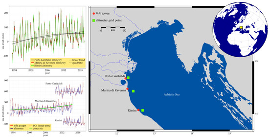
In this paper, we analyze the sea-level variation for the E-R coastal area by selecting three sites along the E-R coast: Porto Garibaldi, Marina di Ravenna, and Rimini (Figure 1). These are the only sites where a TG in operation currently exists. For each site we also identify the closest SA altimetry cell to put the RSL observed at TGs in the framework of the ongoing ASL for the region. TG times series cover different time spans, and this complicates the analysis. The main objectives are: (i) to verify the consistency of different instrumental sea-level records (TG/SA) at each site, by comparing in situ data with the latest CMEMS (Copernicus Marine Environment Monitoring Service) altimetry products (see Section 3); (ii) to observe and analyze differences among obtained sea-level data at the three sites, i.e., at the coastal scale, with a focus on the local variability, heavily influenced here by VLM; (iii) to assess the recent (last 25 years) sea-level change and if it can be assumed as a reference for the E-R region, also highlighting the variability of sea-level rates which strongly depends on the records length and (iv) to discuss this figure in the framework of similar studies at the basin-scale (Adriatic/Mediterranean), and of climate change-related processes. The determination of current sea-level rise at regional scale remains a complex task especially when only short time series are available. However, since this remains a crucial point in support of coastal hazard evaluation and related management/adaptation policies, efforts should be made to understand sea-level variability and to describe its intricacy from the coastal and basin perspective. The paper is organized as follows: Section 2 introduces the study area, Section 3 and Section 4 are dedicated to the description of data and analysis, respectively. Results are presented in Section 5 and discussed in Section 6. Finally, in Section 7, conclusions are drawn.
2. Study Area
The coastal belt of E-R is located in the eastern part of the Po Plain, south of the Po Delta (Figure 1). In geological terms, the Po Plain represents a foredeep basin suffering from natural subsidence. VLMs are mainly due to the consolidation of Quaternary alluvial deposits, with estimated rates along the coastal area of about −1 mm/year and −2.5 mm/year to the south and north of Ravenna municipality respectively, and twice as much at the Po river Delta [50]. Long-term VLMs due to tectonic component have been taken into account by Ferranti et al. [51] and Antonioli et al. [52,53] with rates in the order of −0.95 mm/year since the Last Interglacial (last 125 kyrs) for the northern E-R coast, while −0.22 ± 0.05 mm/year represents the glacio-hydro-isostatic contribution estimated by different GIA models [48]. Since the second half of the 20th century, the subsidence rate in the area has been markedly enhanced by the withdrawal of groundwater and gas extraction [54], with rates locally exceeding the natural subsidence by one order of magnitude. This caused land settlement locally exceeding 100 cm in a few decades [55]. The following gradual decrease in subsidence observed for almost the whole E-R coast is commonly attributed to the groundwater withdrawal cessation, occurred since the 1970s e.g., [54,56], and it has become more evident in the last two decades [55,57]. Current estimates of VLM based on the regional high-precision levelling network, regularly monitored since 1983 by the Regional Agency for Prevention, Environment and Energy of the E-R region (ARPAE), indicate average subsidence rates in the order of 5 mm/year for the last 15 years, decreasing to 3–4 mm/year in the period 2011–2016 [55]; however, peak values in the order of about 20 mm/year are still locally observed in the Ravenna coastal tract. The Coastal Geodetic Network is now the base for the definition of the orthometric heights along the E-R coast [58], integrated with InSAR techniques and GNSS measurements. Recently, Montuori et al. [59] integrating GNSS and multitemporal DInSAR techniques for the monitoring of land subsidence processes along the coastal plain, obtained average rates >3 mm/year, increasing to over 5 mm/year for Ravenna and some tracts along the SE coast. Rates of land subsidence for the Marina di Ravenna dock (from 1970 to present) based on geometric levelling, InSAR techniques and GNSS measurements, are compared by Cerenzia et al. [60].
From a morphological point of view, the E-R coast is represented by fine to medium-sand low-gradient dissipative beaches, 60% of which is the seat of hard protection structures [55]. The E-R coast is in general affected by low-energy waves, with Hs commonly below 1.25 m and microtidal regime [61,62]. The main storms come from the Bora (northeast) and Scirocco (southeast) winds, resulting in storm surge levels >1 m on a 100-year return period [48]. This is a huge concern for such low-elevation coastal zones, exacerbated by forthcoming climate change effects.
The E-R coast faces the northern Adriatic basin (Figure 1), a shallow sub-basin (a few tens of m of depth) with a low topographic gradient. The Adriatic is a narrow epicontinental shelf (800 by 200 km), communicating with the Ionian Sea through the Otranto Strait (Figure 1). The sea-level variability in the Adriatic Sea significantly differs from the other Mediterranean Sea sub-basins because of its setting [63,64,65]. It is dominated by cyclonic circulation driven by wind and thermohaline currents, mainly represented by three gyres centered in the southern, middle, and northern sector of the basin; northerly and southerly currents flow along the eastern (Eastern Adriatic Current, EAC) and western (Western Adriatic Current, WAC) coast, respectively (Figure 1) [64,65,66,67]. Previous analyses of sea-level rise in the altimetry era found an average rate of 3.2 ± 0.3 mm/year over the 1993–2008 for the Adriatic Sea, not uniform on the whole period, but positive (9 ± 0.5 mm/year) between 1993 and 2000 and negative (−2.5 ± 0.5 mm/year) between 2001 and 2008 [68]. Similar positive and negative rates before and after 2001 result for the (basin-average) steric component of sea level, which is correlated with Adriatic Sea level. For the northern sector of the Adriatic, rates of 4.25 ± 1.25 mm/year for the period 1993–2015 [69] and of 3.00 ± 0.53 mm/year for the period 1993–2018 [70] have been recently estimated.
3. Data
In situ sea-level signals are achieved from the three TGs currently operational along the E-R coast (Figure 1). These are installed at Porto Garibaldi (TGPG), Marina di Ravenna, also known as Porto Corsini (TGRA), and Rimini (TGRN). In particular:
TGPG has been operational since July 2009 and it is co-located with a permanent GNSS (Figure 1) station (GARI) that provides VLM information for this site. Different sources are freely available for geocentric surface velocity data at GARI [71]. In this work we considered the GARI time series produced with the INGV (Istituto Nazionale di Geofisica e Vulcanologia) solution by employing the GAMIT/GLOBK software and expressed in the IGS14 (International GPS Service) reference frame [72]. Only TGPG and a portion of TGRA are RLR data retrieved from the PSMSL.
At Marina di Ravenna, different TGs almost continuously collected relative sea-level data since 1873 [73,74], with a main gap from 1922 to 1933. Presently, data are managed by the Italian National Tide Gauge Network (Rete Mareografica Nazionale, RMN) which refers TG data to a local benchmark, located at the lighthouse, 150 m apart. TGRA has a large gap between 2016 and 2019 and, for this reason, the time series considered in this work terminates in December 2015. A permanent GNSS station has operated since 1996 close to TGRA [73] and is currently managed by the Department of Physics and Astronomy of the University of Bologna (no open data).
TGRN has been in operation since July 2012, it is managed by Hera Group corporation, and it is not equipped with a GNSS antenna. Despite the shortness of the data and the lack of a co-located GNSS antenna, TGRN is valuable since it provides the only datum for the southern portion of the E-R coast.
Both TGPG and TGRA operate with radar systems technology (the former coupled with a float system sensor, following the Intergovernmental Oceanographic Commission (IOC) directives [75]) while TGRN operates with a differential pressure transducer. Since only float systems directly provide a SSH measurement, seawater density and gravitational acceleration are considered to convert pressure measured by TGRN into sea level, while radar systems are supplied with dedicated hardware and software that directly convert the measures [76]. Regarding the SA, in this study we use the CMEMS daily gridded dataset (SEALEVEL_MED_PHY_L4_REP_OBSERVATIONS_008_051), having a spatial resolution of 0.125 degree x 0.125 degree [77]. This product is processed by the DUACS (Data Unification and Altimeter Combinations System) multi-mission altimeter data processing system, merging data from all the satellites available at a given time [77,78,79,80,81]. We selected the three closest pixels (SAPG, SARA, SARN) to each of the TG (Figure 1), located at about 5, 13, and 9 km from Porto Garibaldi, Marina di Ravenna, and Rimini TGs, respectively. Each time series was downsampled from daily to monthly by computing the average for the whole samples of each month.
4. Analysis
To minimize the contrast between SA and TG time series, some procedures need to be considered, depending on the purpose of the study. DAC correction in SA (see Section 1) accounts for the low-frequency response of the sea surface to the atmospheric loading, known as the Inverse Barometer (IB) effect [82], and for the high-frequency (HF) response to wind and pressure forcing effect [83]. Since CMEMS products data are corrected by the DAC, the IB and HF effects must be subtracted from TG data for comparison purposes. However, the HF effect is negligible on periods longer than 10 days, hence no correction is needed when monthly averaged data are used [23]. The correction for the IB effect allows the subtraction of the atmospheric loading contribution from the observed RSL at TG. The IB effect correction considered in this work is based on the Wunsch and Stammer [82] formula:
where Δrdry(θ,λ,t) and −1013.3 are the local and global (standard) atmospheric pressure (in millibar) respectively, and −9.948 a constant that accounts for the water density and gravitational acceleration. The monthly mean time series of atmospheric loading at each TG was recovered from the ERA5 reanalysis [84] developed by the European Centre for Medium-Range Weather Forecasts (ECMWF). Furthermore, the application of the GIA correction on TG time series is considered of great importance when reconstructing the ASL, since no worldwide TG record can be assumed to be completely unaffected from the GIA effect [85]. However, since we are interested in studying the local RSL change with respect to the ASL change, and since we are considering short-lived time series, we can neglect to apply this correction.
IB(θ,λ,t) = −9.948 (Δrdry(θ,λ,t) – 1013.3)
Assessing the rate of sea-level variations is a complicated task exacerbated when time series are short and possibly affected by multi-annual and decadal oscillations, difficult to determine on the short term. However, we stick on standard trend assessment by means of ordinary least squares (using NumPy’s Python library [86]) to ease the comparison with previous results even though we are conscious that more sophisticated analysis could provide different results and that this approach neglects the autocorrelation of the time series. This weakness is compensated by the characterization of the periodic signals using two separate approaches, first we compute the Lomb–Scargle periodogram [87,88] (LSP) for each time series to provide a complete description of the frequency content by using the Lomb package [89] implemented in R [90]. Then, we apply the Empirical Mode Decomposition (EMD) method [91,92], a standard method for splitting non-linear and non-stationary time series into a limited sequence of empirically orthogonal “intrinsic mode functions” (IMFs) that describe cyclic modes not necessarily characterized by a constant amplitude nor phase. Differently from traditional spectral methods, the EMD is not requiring assumptions on the functional expression of the regression model. This allows us to decompose each time series in sequence of IMFs plus a residual. The latter, normally monotonic, helps to define how a linear trend is a good model for the non-periodic component of each time series. The significance of the resulting trends is discerned by means of standard test [93] that checks the probability of the null hypothesis to be true. This test is reported beside each trend with its significance code: *** p < 0.001; ** p < 0.01; * p < 0.05; ° p < 0.1; ‘ ‘ (blank) p < 1.
5. Results
5.1. Sea-Level Assessment
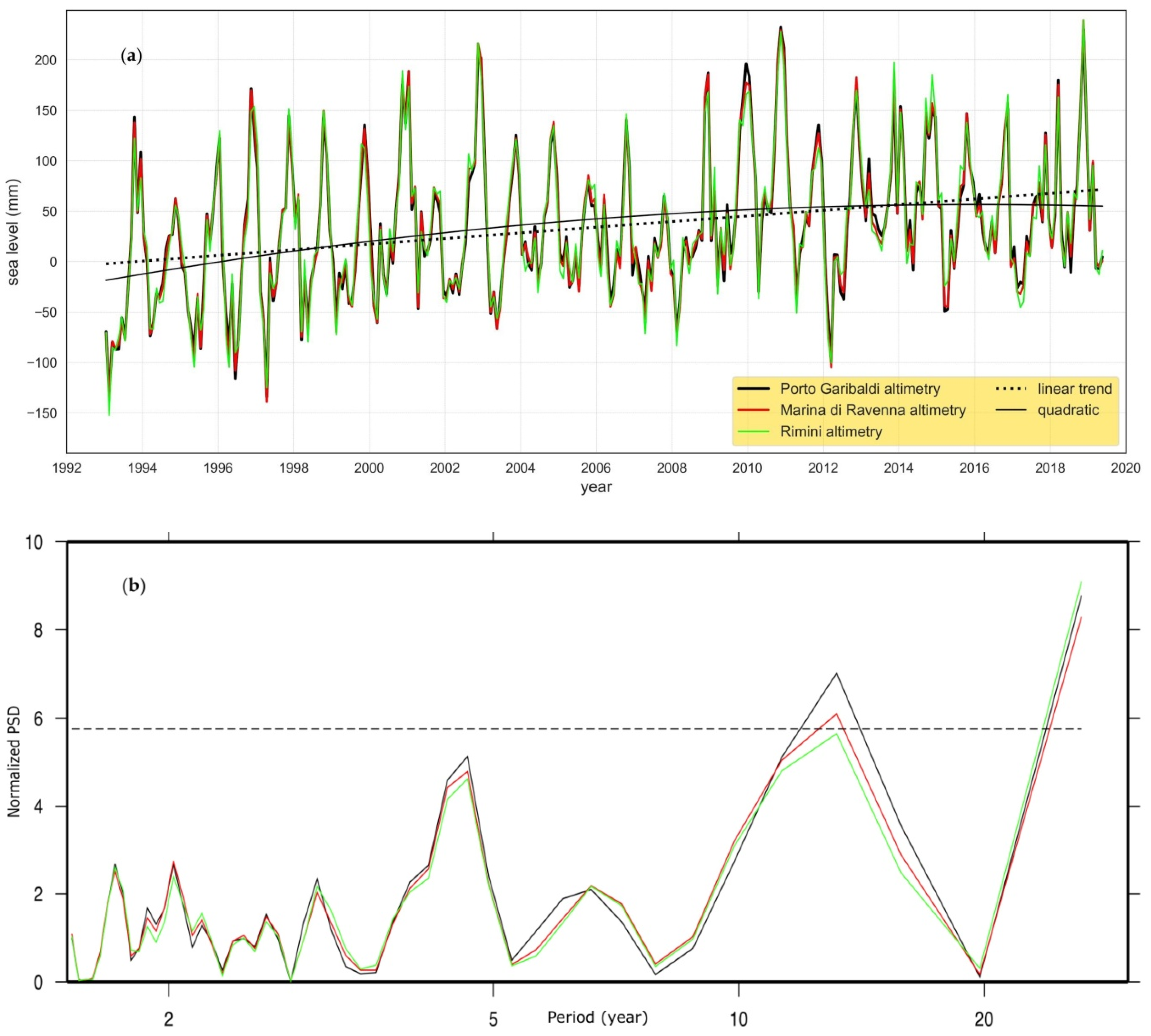
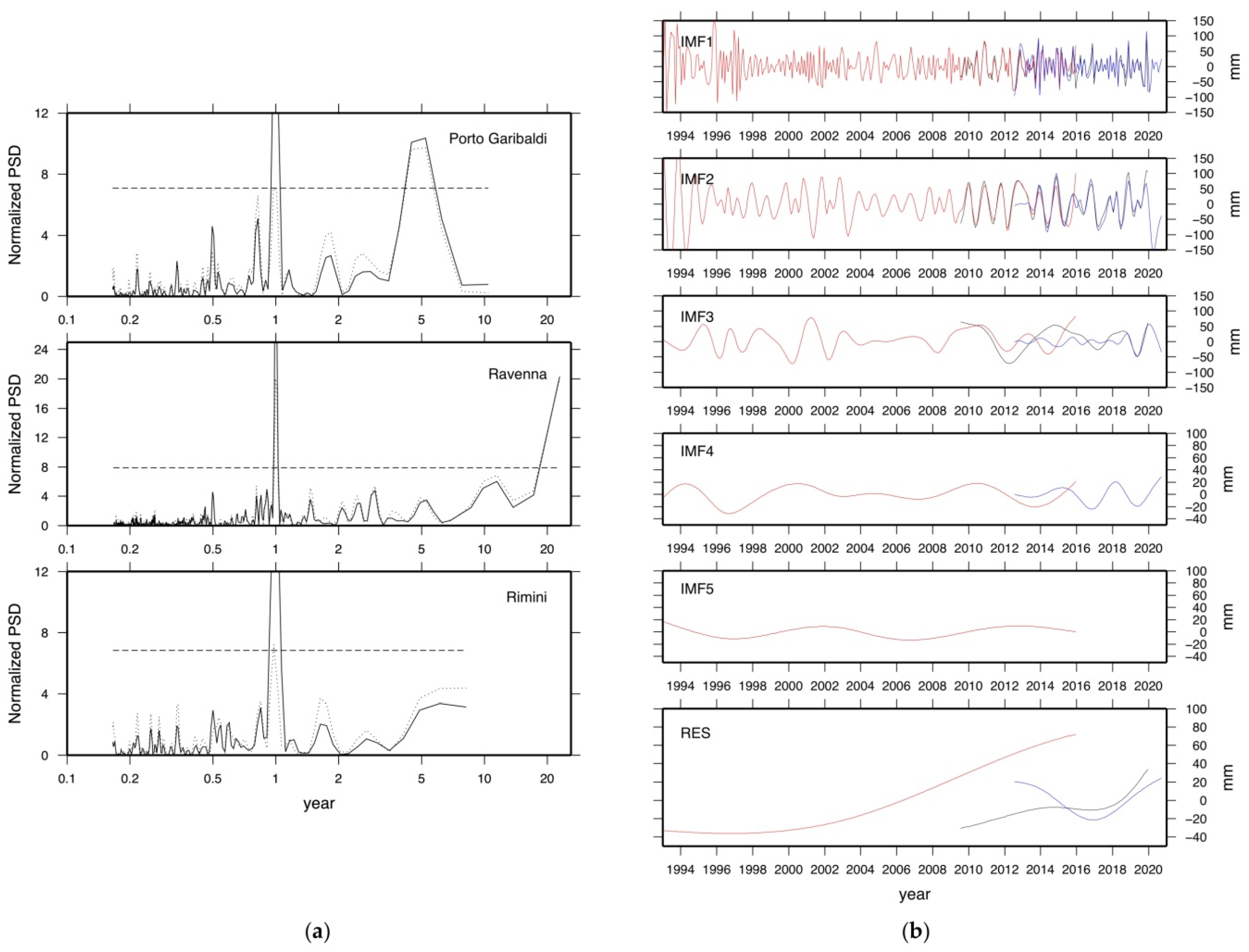
Satellite altimetry time series (SAPG, SARA, SARN) are shown in Figure 2a. The visual comparison among the three SA time series highlights excellent coherence that is confirmed by the correlation coefficient [94] r = 0.98. To better characterize the frequency content of these time series we compute the Lomb–Scargle periodogram (LSP; Figure 2b) for each of them [87,88]. The time series are dominated by the annual and semi-annual oscillation, both related to the seasonality, with peak-to-peak amplitude varying in the order of 150–300 mm (Figure 2a). The resulting LSPs (Figure 2b) also confirm the coherence between the three sites and demonstrate the presence of multi-annual oscillation whose most relevant periods are about 4 and 12 years (see Section 6.1 for detail). LSP significance analysis indicates a small probability (<10%) for the peak at about 12 years to be artefact even though the large sample spacing prevents an accurate definition of the period itself. Conversely, the random peak probability is larger than 10% for the one at about 4 years.
Standard linear regression provides a coherent rate of 2.8 ± 0.5 mm/year over the timespan January 1993–May 2019 (details in Table 1). These values are smaller but comparable to the global average (in the range of 3.1–3.4 mm/year [95]) over the same timespan. The rate assessed in our analysis is smaller than what observed for the northern sector of the Adriatic for the period 1993–2015 (4.25 ± 1.25 mm/year) by Vignudelli et al. [69] even though the two error bars partly overlap, and consistent with what observed for the period 1993–2018 (3.00 ± 0.53 mm/year) by Mohamed et al. [70]. We in fact observe that when fitting the same time series with a second-order model (quadratic, Figure 2a), we get a slight but statistically significant negative acceleration of −0.3 ± 0.1 mm/year2. This local negative acceleration, in contrast with that at the global scale for which a slight positive acceleration (0.084 ± 0.025 mm/year2) has been observed [4], is discussed in Section 6.3.
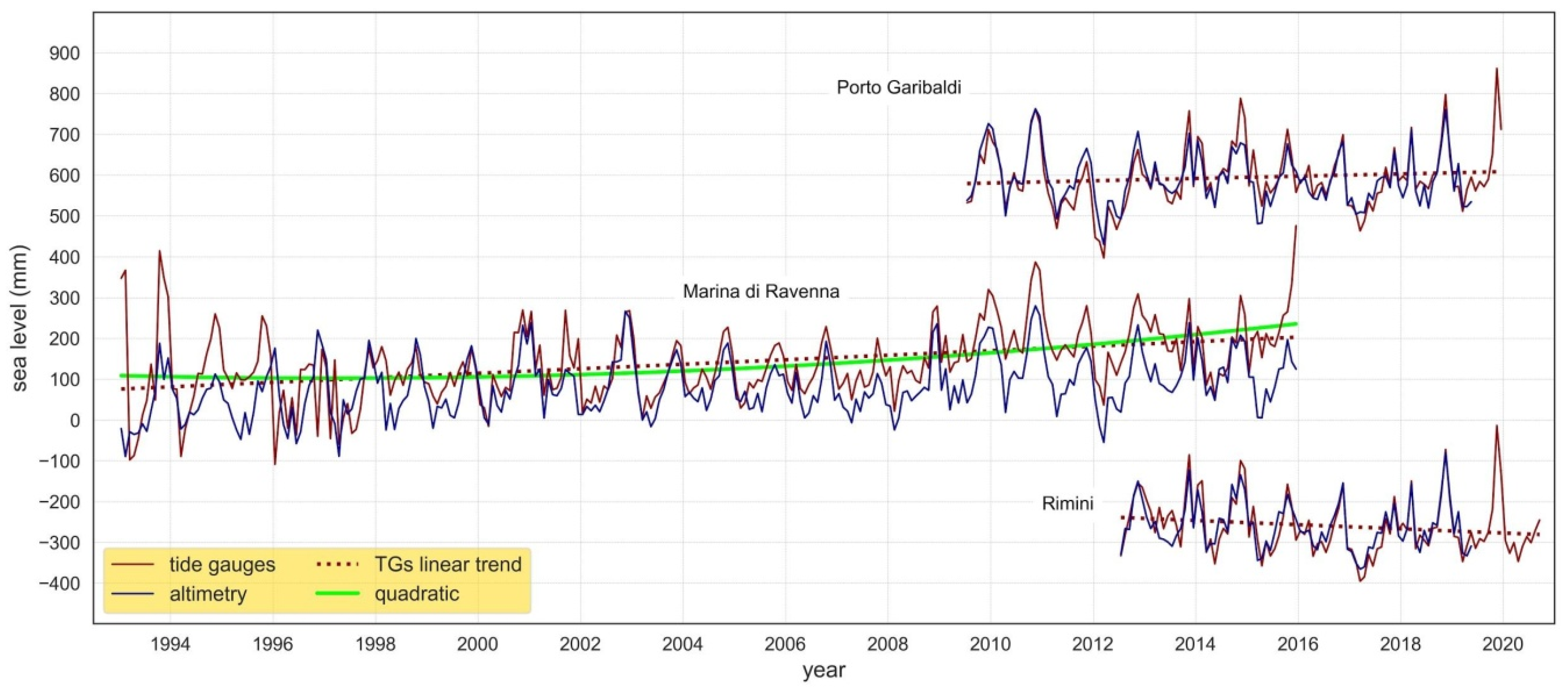
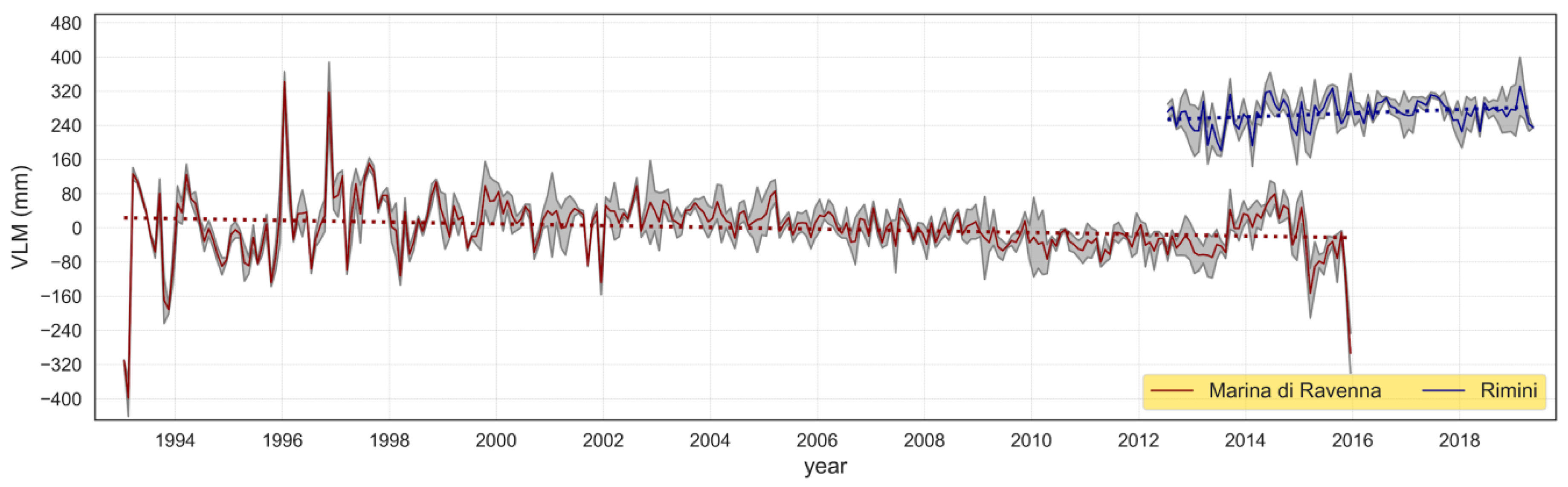
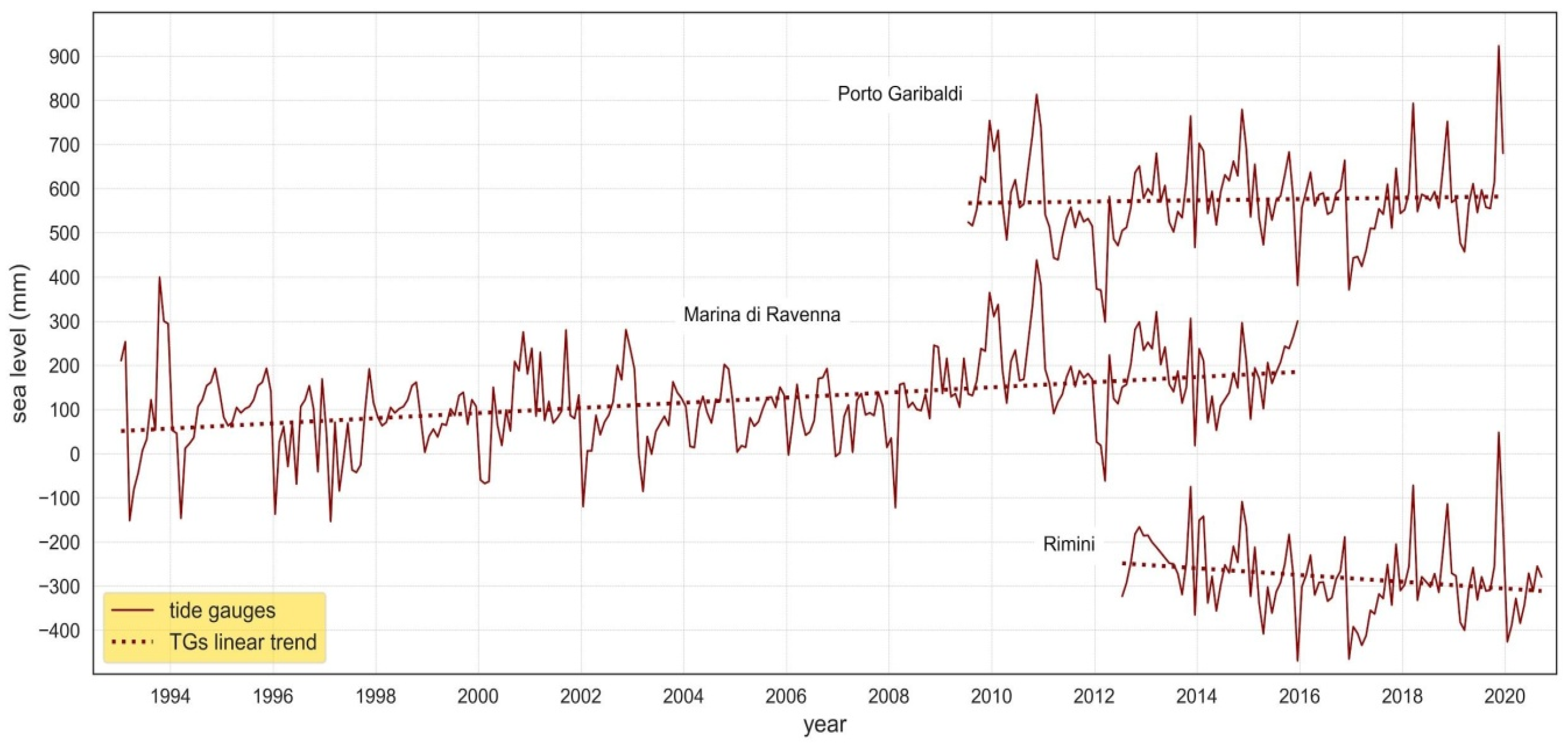
As summarized in Section 3, the three TG time series do not cover the same timespan and are shorter than SA (Figure 3 and Figure A1). This limits the comparison between different sites and, for the shorter one, the reliability of the RSL rate assessment. The longest time series is TGRA (January 1993–December 2015), showing a RSL rate of 5.8 ± 0.8 mm/year (Table 2). This value is consistent with previous studies e.g., [60,68] and significantly higher than the ASL rate observed offshore (January 1993–May 2019, Table 1), as a consequence of the strong vertical land motion expected in this coastal sector. The rate from TGPG has a large uncertainty that leaves the null hypothesis (absence of trend) likely, while from TGRN it is largely negative. Despite the large disparity in the resulting RSL rate is also a consequence of the different time spans, we note that the correlation coefficient, restricted to the overlapping periods, is 0.80 between Porto Garibaldi and Marina di Ravenna, 0.94 between Porto Garibaldi and Rimini, and 0.77 between Rimini and Marina di Ravenna.
Since one of the goals of this study is the comparison between RSL and ASL to better understand the different governing mechanisms and observational approaches, we apply the IB correction to the raw TG data to compare them with SA time series (corrected for DAC). This correction gives a valid reprocessing of the sea-level variability without the meteorological effect influence [96]. We can observe that the IB correction leads to a reduction, in amplitude, for most of the extrema (Figure 3 and Figure A1) and this reflects in smaller variance for the residual of the OLS regression and, indeed, in a smaller error associated with the trend (Table 2). As expected, the IB-corrected TG time series result in different RSL rates and smaller uncertainties. We also note that the quadratic fit for TGRA returns a positive acceleration (0.7 ± 0.3 mm/year2), not present in the ASL data (Figure 3).
The SA time series have been shortened to match each of the three TG time series (Figure 3). Also in this case the correlation coefficient is high (0.89) for Porto Garibaldi e Rimini and moderate for Marina di Ravenna (0.66). We notice that the rates for the shortened SA time series (Table 3) differ from what observed for the complete time series (January 1993–May 2019). In particular, in the case of SAPG and SARN, for which we consider only the last part of the time series, rates turn negative. In details, for SAPG (timespan July 2009–May 2019) the trend is negative, while the corresponding rate of RSL is positive (Table 3). This result for SA linear trends is not unexpected since it is consistent with the observed negative acceleration (Table 1) that suggests a decrease in ASL rate of about −5 mm/year over the removed 16 years (1993–2009). For the same reason, at SARA the trend for the period January 1993–December 2015 is larger than the one computed for the whole SA timespan, and lower than the RSL rate (Table 3). Finally, for the case of Rimini, SARN trend is negative (Table 3) but the large error bar demonstrates that the null hypothesis (no trend) could not be rejected with 0.1 < p < 1. In other words, the large error bar demonstrates the low significance of the linear model and that the rate could also be null or even positive. As in the case of altimetry, the analysis of shorter-term time series also modifies the TG trend values (compare Table 2 and Table 3), except for TGRA whose time series is fully covered by the altimetry and therefore does not need to be cut. Furthermore, an important contribution to the local sea-level variation at different sites is represented by the vertical movements (VLM) component included in the TG data. This will be taken into account and discussed in Section 6.2.
5.2. Periodic Signals
The large uncertainty in estimated rates, and in their variation over different time spans, suggests analyzing the periodic components of the time series and to define their relevance in terms of amplitude and frequency to better constrain the characteristics of the sea-level change. With an approach similar to that used in Section 5.1 for SA, we analyze the TG time series by means of LSP and EMD.
Results are shown in Figure 4. LSP analysis (Figure 4a) for the whole period range confirms the prominence of the oscillation at 1 year (especially for longer time series), while at shorter periods (below 1 year) different peaks emerge between 0.2 and 0.5 years (i.e., between 2 and 6 months). For the case of Porto Garibaldi and Rimini we notice that the IB correction enhances the signal for the annual oscillation and that a clear peak emerges at 0.85 years (10 months). This partly contrasts with what observed for the LSPs computed for the SA time series in which the semi-annual oscillation emerges more clearly. The ascending termination of the periodograms at the longest period (right side) for the case of TGRN and TGRA could reflect the presence of periodic signals at periods longer than the timespan covered by this (very short) time series. We also notice that IB correction reduces the power amplitude at longer periods.
To better discern the periodic signals from the long-term trend, we also applied the EMD analysis to each IB-corrected time series. From Figure 4b, we note that at high frequency (IMF1–2), large non-sinusoidal oscillations exist, and these show an overall coherence between the three sites. This suggests a regional scale origin. IMF3, whose periodic signals range between 1.5 and 3 years, is not coherent during the overlapping timespan, pointing to a site-related effect. IMF4 exists only for Marina di Ravenna and Rimini but these time series overlap for a very short timespan and this prevents any comparison. IMF5 at even longer periods emerges only for Ravenna and it demonstrates an almost sinusoidal oscillation with a period of about 10.7 years. Residuals confirm what observed from linear regression (Table 3) and introduce some more complexity: Marina di Ravenna shows short-lived positive acceleration around year 2000, Porto Garibaldi is almost linear with two minor inflections, while Rimini shows a parabolic shape contrasting with a linear model. For Rimini, the shortness of this time series limits the distinction between a branch of a parabola or of a sinusoid with period of about twice the length of the time series.
6. Discussion
The above data analyses provide a complex picture for the sea-level variation along the E-R coast. Actually, different data and processing, and the large literature available for the region suggest several perspectives for discussing and interpreting such complexity. In this section, we propose a comprehensive interpretation of our results, also in the framework of previous studies. We focus on factors affecting sea-level variability, on the role of the VLM in the E-R coast, and on the difficulties of providing a figure for the current or recent rate of sea level for the area.
6.1. Sea-Level Time Series and Rates for the E-R Coast
To verify the consistency of different instrumental sea-level records at the coastal scale, TG and satellite altimetry time series were analyzed at three sites along the E-R coast. Altimetry time series at the three sites turn out to be very consistent, showing basically the same rate of sea-level rise (Figure 2a; Table 1) and variability in the last 25 years, also denoted by a perfect correlation among them (r = 0.98). On the other hand, the results provided by the three TGs are more variable in terms of trend and variability both among them and with respect to the altimetry. This can be the consequence of some critical factors. First, the TG time series cover different time spans (Figure 3), and this can cause discrepancies in the observed rates (Table 2 and Table 3). Indeed, the timespan for which the three TG time series overlap is very short, thus preventing a reliable comparison. Secondly, rate assessments based on short records are particularly sensitive to oscillations especially at their extremes, thus they are not suitable for deriving climatological-related information in the long term [2].
It is a common practice to reproduce the sea-level variation over time by a linear model. However, this approach sometimes forces the observed phenomenon into a model that is too simple, neglecting periodic and aperiodic variations of different time scale and size that can bias the resulting trend. The addition or subtraction of a few samples at the time series extrema can cause considerable variations of the trend rate as recognizable by comparing values listed in Table 1 and Table 2 with those of Table 3. For the case of the Adriatic Sea, the rate of sea-level rise strongly varies with time because of the chosen record length [68,85,97,98], and by the contamination of seasonal and inter-annual variability [99]. To constrain this, we combined EMD analysis and LSP periodograms. LSP, among the expected annual and semi-annual oscillations, demonstrates two oscillations at about 4 and about 12 years for SA data, while the interpretation of TG data is more complex given the short timespan for TGPG and TGRN. TGRA shows a more complex periodogram in this band, suggesting that several events contribute to hinder the SA peaks; however, EMD analysis returns a period signal at about 10.7 years. We can speculate that this oscillation and the SA peak at about 12 years are comparable with the 10 years-oscillation at Mediterranean scale observed by Bonaduce et al. [100].
The oscillations that influence the Adriatic Sea are mainly due to cycles that act at annual (stronger energy signal), semi-annual (6 months) and inter-annual (5 years and higher) scales [101], as also demonstrated in our data (Figure 2a and Figure 4a). The whole Mediterranean basin is also influenced by oscillations at lower frequencies driven by natural modes, which produce intermittent anomalies in the long-term rate. As analyzed by Galassi and Spada [45] the NAO and AMO power are mainly concentrated at a period of about 8 and 9 years respectively; they also pointed out that the AMO strongest signal is found at multidecadal periodicities, i.e., between 50 and 70 years. Moreover, one of the most energetic modes of variability in the Adriatic basin is linked to the periodic occurrence (approximately 20 years) of opposite phases of the NAO and AMO [45] which produce a large scale zonal atmospheric gradient [102] and a sea-level non-steric fluctuation directly linked to mass transport through the Strait of Gibraltar driven by wind [39,103]. The last occurrence of this phenomenon was determined as the cause of the large positive anomaly recorded in sea-level signal during 2010–2011 [40,70] by all Mediterranean TG stations [100]. Indeed, the right site upgoing termination of the LSPs (Figure 2b and Figure 4a) could be an indicator of a longer period oscillation that could not be quantified here because of the length of the time series.
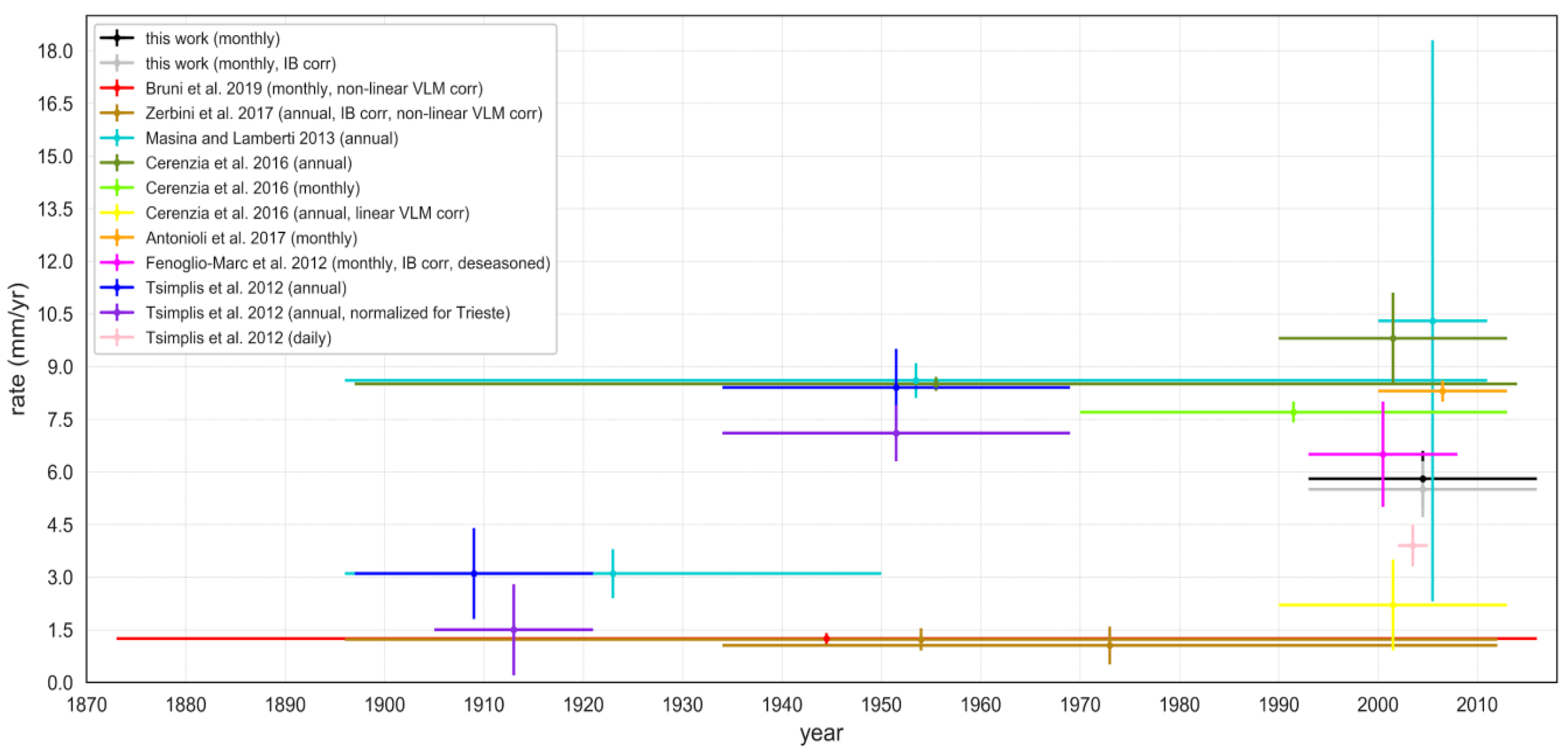
One further cause of the variability in SL rate and corresponding uncertainties is the different data processing and different corrections applied. An example of the above cited complexity is the Marina di Ravenna site for which several previous studies exist, based on the same TG time series but using different methodologies and adopted corrections, as shown in Figure 5 where the results of some of the most representative studies conducted on TGRA are summarized (see also Table A1). There is a relation between the time series length and the error size of the trend resulting from OLS regression, i.e., the error scales inversely with the number of samples of the analyzed time series [104]. Rate for longest datasets generally agree, but only when similar data corrections are applied: Zerbini et al. [73] and Bruni et al. [74] removed from data the non-linear VLM resulting from GNSS data, while Cerenzia et al. [60] accounted for the linear VLM (from various geodetic data), and Tsimplis et al. [41] normalized the data with respect to the TG time series of Trieste (considered to be a tectonic stable site). Rates computed from long time series without VLM correction are significantly higher [41,60,105] but still relatively grouped. By contrast, rates from short time series (i.e., less than 20 years, see [60,68,105,106]) denote extreme variability and inconsistency between them regardless of the corrections applied, e.g., IB correction and deseasoning, whose influence is relatively low here with respect to the crustal movements corrections. This highlights how the natural variability and the contribution of VLMs strongly influences the RSL signal at the TGs, preventing the estimate of a univocal sea-level trend valid at the short-, middle-, and long-term scales. Given the short time spans and the described complexities, we thus cannot establish if and how the observed trends could be representative of the long-term rate of RSL rise. Also, the time series analyzed in this work (Figure 3; Table 2) suggest that a not constant rate of subsidence might play a crucial role in the observed RSL change at this time scale.
Regarding the comparison between the two different techniques, the analyzed SA and TG records have been downsized to cover only the overlapping timespan at each site and this causes differences in the estimated rates at the three sites (Table 2 and Table 3). The results of this comparison are thus expected to improve in the next years/decades when the available time series will be longer for the analyzed sites. An 18-year- [107] or 15-year-long [108] recording is needed to obtain a good correlation. It has been shown, in fact, that over intervals shorter than 10 years the inter-annual variability affects more the rate of global mean sea level from TG than from altimetry [68]. However, despite these considerations, we obtain very high correlation between SA and TG sea-level time series at the three studied coastal sites. In particular, the three downsized SA time series show a strong correlation with the IB-corrected TG time series (Figure 3), especially at Porto Garibaldi and Rimini (r = 0.98). This confirms the good quality of the chosen SA product that, as suggested by Vignudelli et al. [69] for the northern Adriatic Sea, is less affected by degradation at the coast than previous SA data. As a matter of fact, different linear rates result for TG and SA at each of three study sites (Table 3). Since SA provides a coherent rate along the E-R coastal area (Table 1), an important contribution to the spatial variability of RSL at different sites should derive from the VLM component included in the TG data, and this is the focus of the next section.
6.2. The Role of Vertical Movements in Sea-Level Determination
In the E-R coastal area (and on a great portion of the Northern Adriatic coast, Italian side) subsidence is widespread and occurs at high rates [109], while vertical deformations caused by other phenomena as GIA are more than one order of magnitude smaller than subsidence that here dominates the VLM affecting RSL change [60,68,69,105,106,109]. Presently, different integrated techniques, such as high-resolution levelling, e.g., GNSS and InSAR, provide data on VLM with increasing accuracy [57,58]. However, the small size and short-lived variation of vertical deformation processes causes this information to be not always comparable/homogeneous. Furthermore, the common practice of co-locating a GNSS station at the TG site is relatively recent and many TGs do not have associated VLM data with the necessary precision.
As mentioned in Section 3, TGPG has co-located GNSS station (coded name GARI) since Jul. 2009. GARI station provides well constrained VLM data well reproduced by a linear trend with rate equal to −2.8 ± 0.1 mm/year. At Marina di Ravenna, the VLM rate estimated for the GNSS station located close to TGRA, estimated through the Gipsy software over the timespan July 1996–December 2015, is −5.6 ± 0.2 mm/year [110]. These VLM rates, when compared with rates of RSL at each site well explain a relevant portion of the sea-level change in the considered time frames (Table 2) while the ASL contribution seems low or negligible. At Rimini, the rate of RSL in the time frame Jul. 2012–Sep. 2020 (the only one available at TGRN) is negative (−5.1 ± 3.0 mm/year; Table 2), in contrast with what observed for TGRA and TGPG. Here, a GNSS station (ITRN) operated by the Coastal Geodetic Network [57] (located at 2.6 km from the tide gauge, at 44°2’54”N 12°34’55.4”E) shows a VLM rate almost null (0.00 ± 0.8 mm/year) for the period 2011–2016 (for further details see [111] and references therein).
Integrated data on vertical deformations (topographic levelling, GNSS and InSAR) of selected benchmarks of the E-R Coastal Geodetic Network and data previously acquired in the framework of the Regional Network for subsidence monitoring [112], provide gradually decreasing subsidence rates for all the coastal sites under study in the last 25 years [55,57] (Table 4). These data are gridded at 100 m × 100 m and reproduced as isokinetics of VLM at the regional scale; associated error is estimated as ±2 mm/year [57]. For the area that contains the TG data, rates summarized in Table 4 can be considered representative of the subsidence. Actually, these data agree with the rate observed by GNSS at Porto Garibaldi and Marina di Ravenna. For Rimini, subsidence data suggest that this phenomenon is gradually decreasing but not inverted, as the negative rate of RSL rise might suggest.
As a parallel approach, we use the SLE (Equation (1)) to compare the observed sea level or ground variation with the one obtained by the combination of the over two data. It must be pointed out, however, that the accuracy of this method is frequently larger than 1 mm/year whatever its application [113,114,115]. Despite the coarseness of this method (20 years of data should be required to yield a high-precision estimate, [115]) several authors have applied it to regional studies, since understanding VLM for sea-level research is of farthest significance e.g., [21,116,117,118,119,120,121,122,123,124].
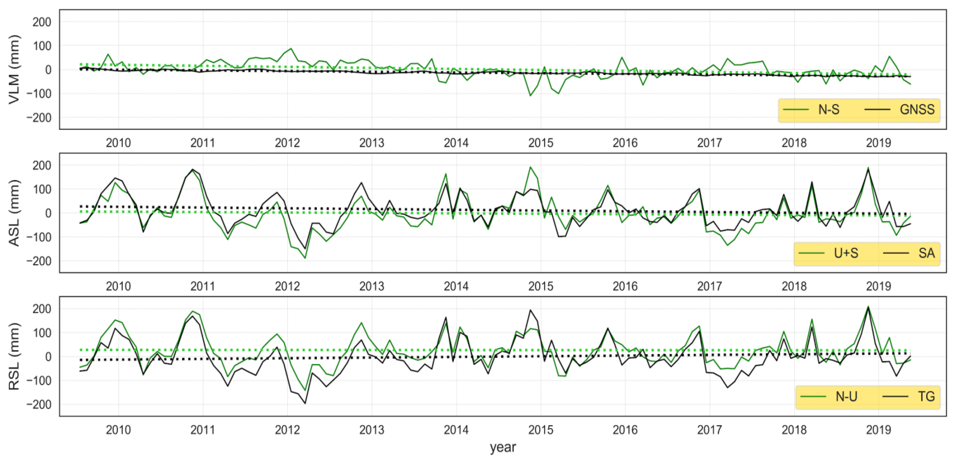
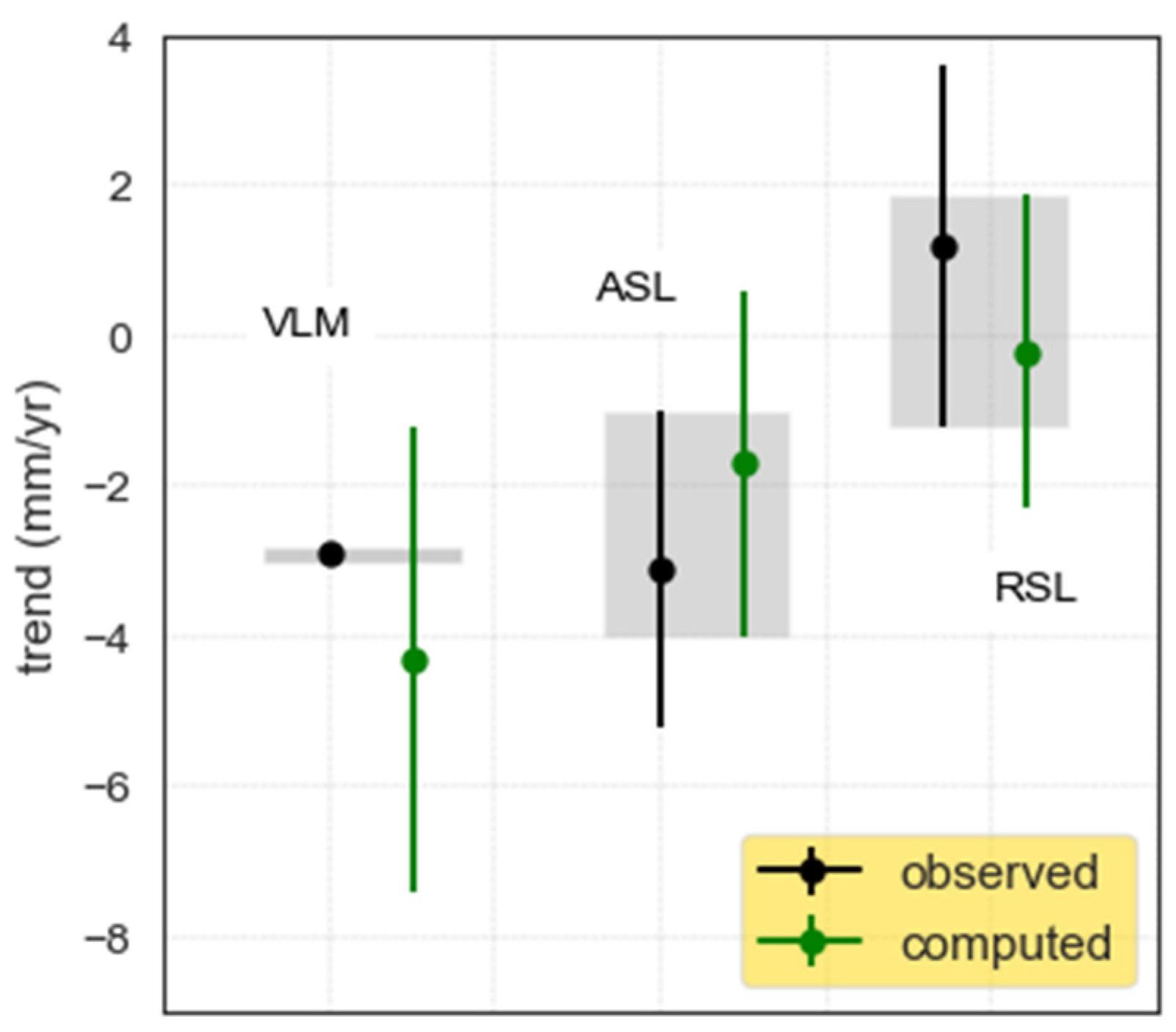
For the case of Porto Garibaldi, the three variables that form Equation (1) are available from the different observables considered for this work over the common period July 2009–May 2019. This allows us to evaluate the different estimates obtained through the two approaches, i.e., by comparing the rate obtained from the linear regression of the direct observation (Table 3) with those computed by using Equation (1) (hereafter computed). Visual inspection of Figure 6 suggests a strong correlation between the pairs (SA, U+S) and (TG, N-U), this confirmed by r = 0.90. By contrast, the correlation between (N-S) and the GNSS is low (r = 0.37). This follows the different accuracy of GNSS data (below 0.1 mm/year) with respect to TG data contained in N-S. The trend values related to the computed time series (Table 5) slightly differ from those of the observed one (Table 3). We note that only for U the null hypothesis (no trend) could be rejected. Figure 7 shows that the observed and computed trends match within their error bars, despite the differences between their central values, suggesting a good coherence between the different observations. In particular, the trend observed for N (from U+S) is lower in value than the ASL derived from SAPG (−3.1 ± 2.0 mm/year) even though their error bars overlap (Figure 7). The trend for S is almost null and its error bar shows good overlap with the rate of RSL given from TGPG (1.2 ± 2.3 mm/year; Figure 3, Figure 6, and Figure 7). U is affected by larger uncertainties with respect to the GNSS time series, with uncertainties lower in value (−2.9 ± 0.1 mm/year in the time frame Jul. 2009–May 2019) and completely contained in the U error bar (Figure 7).
For the case of Marina di Ravenna and Rimini, only S and N can be directly determined, since GNSS instruments are not co-located at these TGs. Then, Equation (1) can be applied to indirectly estimate U. Figure 8 shows the time series (SA-TG) for Marina di Ravenna and Rimini (with their related errors) whose rate (Table 5), according to Equation (1), should represent (U = N − S). These values are quite unexpected since subsidence at Marina di Ravenna is known to be larger (see Table 4); at Rimini this contrasts with the observed subsidence (Table 4). However, if U for Marina di Ravenna is computed on the reduced timespan for which GNSS data exist (July 1996–December 2015) the rate of VLM is −4.7 ± 0.6 mm/year, smaller than that provided by the GNSS located near TGRA (−5.6 ± 0.2 mm/year). The two results do not match within their error bar for only 0.1 mm/year. As mentioned above, this GNSS is in the vicinity of TGRA and, the larger the distance between GNSS and TG, the smaller the representativeness of the real VLM at the TG. It has been observed that, when large heterogeneities exist, a few hundred meters of distance between TG and GNSS stations can cause decoupled movements [18]. This seems to be the case for the Marina di Ravenna harbor where Cerenzia et al. [60] found different rates of subsidence at very short distances, likely due to the weight effect of the structures themselves (e.g., the embankment with respect to the dock and the lighthouse). Fenoglio-Marc et al. [68] reports similar results for the Marina di Ravenna site, where GNSS observations provide a higher VLM rate with respect to the one computed from SA and TG difference, attributing it to anthropogenic causes, to the distance between the TG and the closest SA grid point and to the corrections applied on the RSL time series.
At Rimini, the context appears completely different with respect to Marina di Ravenna and Porto Garibaldi. Despite the high correlation between TGRN with SARN, at Rimini the RSL shows a negative trend (Figure 3), although the small timespan covered by TGRN time series gives at this data very low statistical significance (Table 2 and Table 3). The time series (SA-TG) shows a positive trend for U (Table 5) indicating a “proxy-derived” local effect of land uplift (Figure 8), in contrast with the VLM rates (0.00 ± 0.8 for the timespan 2011–2016) provided by the ITRN station. GNSS values agree with recent subsidence monitoring activities using InSAR (Table 4). The error associated with InSAR measure is 2 mm/year, suggesting that for the period 2011–2016, some portion of the Rimini area that includes the GNSS and TG stations may undergo opposite VLMs (uplift) with respect to other sectors of the E-R coastal belt. At Rimini, the GNSS station is located 2.6 km apart from the TG and this makes the data comparison even less effective than for the case of Marina di Ravenna [18]. Measured subsidence at Rimini has markedly decreased in the last two decades [57] and it cannot be excluded that VLM could reverse in the next decades; unfortunately, to date there is not enough data to support this hypothesis and more years of data acquisition are required.
6.3. The Sea-Level Trend Acceleration Issue
As anticipated in the introduction, at global scale the sea level has been rising at a rate of 3.3 ± 0.5 mm/year [3], with a positive acceleration of 0.084 ± 0.025 mm/year2 [4] over the altimetric era (1993–present). Global maps show that the sea-level rise is not spatially uniform, with a diffused pattern of null rate and even showing a sea-level fall, see [125]. Then, it is not surprising that this heterogeneity also reflects in different local sea-level acceleration as for the case of the small spot target of this study in which we observe, for the same period, a negative acceleration of –0.3 mm/year2. Acceleration could be the consequence of global short-lived phenomena, as for the case of the Pinatubo eruption in 1991 [126] or of climatological events. Moreover, given the length of the SA time series, accelerations could be also a consequence of the contribution of multidecadal oscillations for which only a portion of it is sampled. Because of this consideration, the observation of a full cycle (at least) is required to properly model the oscillation itself, determine its origin, and its plausible relation with climate change. Unfortunately, since the satellite altimeter era only started in 1993, and long-term TG observations are contaminated by an unknown non-linear VLM (measured only since co-located GNSS acquisition started, i.e., in the late 1990s), it is currently complicate to properly attribute to the ongoing observed regional sea-level variations to climatological origin. In our case, we observe a localized negative acceleration for the E-R coast, whose interpretation should be put in the broader context of the Mediterranean Sea in which a marked spatial variability of sea-level trend is observed, for instance, by Bonaduce et al. [100]. The ASL negative acceleration observed at the E-R coast in recent decades (Figure 2a; Table 1) has been previously noted by other authors. After a positive acceleration of sea-level rise observed in the Mediterranean Sea during the 1990s [127] since the early 2000s, in fact, the sea level stopped rising [128,129,130]; this seems to match well with the quadratic fit shown for SA in Figure 2a. As previously explained in Section 6.1, ocean–atmosphere oscillations are responsible for inter-annual and interdecadal cyclic sea-level variations in the Mediterranean; the main engine of these phenomena has been associated, at a global scale, with natural modes (e.g., the NAO and the AMO) inducing temporary reductions or magnification of sea-level trend amplitude at the basin to regional scale [103]. Besides this inter-annual variability, changes in sea-level acceleration on multidecadal time scales have been documented by several authors for the whole 20th century which is generally characterized by a greater rate in the first half, followed by an overall negative acceleration [43,131,132,133]; however, the processes causing this variability, and their link to climate change, are not completely understood yet.
We showed in Section 5.1 that the SA time series, shortened for matching with the TG time series (Figure 3), provide rates differing from what observed for the complete SA time series (January 1993–May 2019, Figure 2a). In particular, in the case of SAPG and SARN, rates turn negative (Table 3; although for Rimini the hypothesis of no trend could not be rejected), consistently with the observed negative acceleration (Table 1). For the Marina di Ravenna site, the overlapping timespan (1993–2015) is long enough to obtain, from the quadratic regression, a significant acceleration in the time series (Figure 3). Namely we get 0.7 ± 0.3 mm/year2 for TGRA and −0.2 ± 0.2 mm/year2 for SARA. The opposite signs suggest that two different phenomena govern the two accelerations and a good candidate could be VLM that, as mentioned above, is governed here by subsidence. From Equation (1), the VLM acceleration is the difference between those of the two terms mentioned above, and it results equal to −0.9 ± 0.4 mm/year2. Actually, subsidence is slowing down in the region and locally in the surrounding of TGRA as resulting from Table 1, and this should reflect in a positive acceleration in the ongoing negative VLM. We can then argue that what we are observing at TGRA is something different from the effects of the local subsidence or, more likely, other phenomena are governing the acceleration at TGRA.
At the regional scale, the decrease of subsidence measured by the E-R Coastal Geodetic Network over recent decades (see Table 4) is a favorable indication in terms of reducing future flooding vulnerability for this area. However, as already pointed out by Cerenzia et al. [60] and Fenoglio-Marc et al. [68], and discussed at Section 6.2, different rates of VLM are available, depending on the precise site of measurement and not necessarily representative of the VLM at the TG location. We thus remark the need for local and repeated VLM measurements at the TG site to correctly interpret RSL series and for detecting possible ASL positive or negative accelerations.
7. Conclusions
In this paper, we have studied the sea-level variation along the E-R coast by focusing on monthly sea-level observations from the three available TGs located at Porto Garibaldi, Marina di Ravenna, and Rimini. Data are compared with CMEMS SA data from the three grid points closer to each of the TGs. The combined use of altimetry and tide gauge data (supplemented by GNSS acquisition) is considered, in fact, a promising approach, in terms of precision and cost-effective implementation, to better define various physical processes in the coastal domains and to anticipate the impacts of future rise in sea levels [10,11,22,69,134,135,136,137].
Our results show that the ASL time series (from SA) are coherent along the coastal tract, providing a rate of 2.8 ± 0.5 mm/year for the timespan Jan 1993–May 2019, smaller but comparable to the global average (3.3 ± 0.5 mm/year). Moreover, we note in the E-R coast a negative acceleration of −0.3 ± 0,1 mm/year2 that contrasts with the positive global acceleration. The comparison with the IB-corrected TG time series suffers from the short overlapping period between the two different datasets (Jul. 2009–May 2019 at Porto Garibaldi; Jan 1993–Dec 2015 at Marina di Ravenna; Jul. 2012–May 2019 at Rimini). Despite their shortness, the SA and TG time series show high correlation coefficient (0.89) at Porto Garibaldi and Rimini, and a moderate one (0.66) at Marina di Ravenna. The lower correspondence achieved at Marina di Ravenna, as well as the difference between ASL and RSL rates for this site (Table 3), are mostly associated with the local rate of VLM. Actually, VLM can hamper the detection of signals associated with sea-level change and related spatial variations [22]. For all the three analyzed sites, this remains an important contribution to quantify. It is remarked the need for co-located monitoring of the ground motions at the TG sites, since the determination of VLM is a key element in understanding how sea level has changed over the past century and how future sea levels may impact coastal areas [22].
Finally, as already observed for other coastal areas [11,13,69], the good match between altimetry and in situ observation confirms that high-standard satellite product can provide consistent data even at short distance from the coast. Linking satellite altimetry measurements with tide gauge, by bridging the open-ocean measurements with those in proximity of the coast [12] is part of a new challenge in monitoring sea-level rise along coastal tracts. In this view, the maintenance and implementation of observation stations for continuous monitoring of sea level in the coastal zone is a fundamental tool for coastal management and defense strategies.
Author Contributions
Conceptualization, M.M., M.O. and C.R.; Formal analysis, M.M. and M.O.; Investigation, M.M., M.O. and C.R.; Methodology, M.M. and M.O.; Visualization, M.M. and M.O.; Writing—original draft, M.M., M.O. and C.R.; Writing—review & editing, M.M., M.O. and C.R. All authors have read and agreed to the published version of the manuscript.
Funding
This research received no external funding. Ph.D. fellowship of M.M. is financed through the Strategic Development Project of the BiGeA Department, University of Bologna. M.O. research was partly funded by the Istituto Nazionale di Geofisica e Vulcanologia departmental project MACMAP.
Institutional Review Board Statement
Not applicable.
Informed Consent Statement
Not applicable.
Acknowledgments
The authors would like to thank the Hera Group corporation, the PSMSL and the CMEMS for their support and for making data available. We thank Susanna Zerbini, Enrico Serpelloni, Stefano Gandolfi, Fabio Raicich, Davide Putero, Giorgio Spada, Luciana Fenoglio-Marc, Marcello Passaro and ARPAE-SIMC for helpful feedback on technical and scientific aspects. Marco Anzidei and three anonymous reviewers are acknowledged for their fruitful comments and suggestions that helped improving the paper. This work was supported by the University of Bologna, Ph.D. course in Future Earth, Climate Change and Societal Challenges.
Conflicts of Interest
The authors declare no conflict of interest.
Abbreviations
| AMO | Atlantic Multidecadal Oscillation |
| ARPAE | Regional Agency for Prevention, Environment, and Energy of the Emilia-Romagna region |
| ASL | Absolute Sea Level |
| CMEMS | Copernicus Marine Environment Service |
| DAC | Dynamic Atmospheric Corrections |
| DInSAR | Differential Synthetic-Aperture Radar Interferometry |
| DUACS | Data Unification and Altimeter Combinations System |
| E-R | Emilia-Romagna |
| EAC | Eastern Adriatic Current |
| ECMWF | European Centre for Medium-Range Weather Forecasts |
| ECV | Essential Climate Variable |
| EMD | Empirical Mode Decomposition |
| ENSO | El Niño Southern Oscillation |
| ERF | Effective Radiative Forcing |
| GARI | Permanent GNSS station co-located at Porto Garibaldi tide gauge |
| GCOS | Global Climate Observing System |
| GIA | Glacial Isostatic Adjustment |
| GNSS | Global Navigation Satellite System |
| HF | High Frequencies response of sea level to wind and pressure forcing effects |
| Hs | Significant wave Height |
| IB | Inverse Barometer effect |
| IGS | International GPS Service |
| IMF | Intrinsic Mode Function |
| InSAR | Interferometric Synthetic-Aperture Radar |
| INGV | Istituto Nazionale di Geofisica e Vulcanologia |
| IOC | Intergovernmental Oceanographic Commission of UNESCO |
| IPCC | Intergovernmental Panel on Climate Change |
| LSP | Lomb–Scargle Periodogram |
| NAO | North Atlantic Oscillation |
| NGL | Nevada Geodetic Laboratory |
| OLS | Ordinary Least Square regression |
| PSMSL | Permanent Service for Mean Sea Level |
| RLR | Revised Local Reference |
| RMN | Italian National Tide Gauge Network |
| RSL | Relative Sea Level |
| SA | Satellite Altimetry |
| SAPG | Closest altimetry pixel to Porto Garibaldi tide gauge |
| SARA | Closest altimetry pixel to Marina di Ravenna tide gauge |
| SARN | Closest altimetry pixel to Rimini tide gauge |
| SLE | Sea-Level Equation |
| SSH | Sea Surface Height |
| TG | Tide Gauge |
| TGPG | Tide Gauge at Porto Corsini |
| TGRA | Tide Gauge at Marina di Ravenna |
| TGRN | Tide Gauge at Rimini |
| UNFCCC | United Nations Framework Convention on Climate Change |
| VLM | Vertical Land Movement |
| WAC | Western Adriatic Current |
Appendix A
Figure A1.
Raw TG time series. Dotted lines represent estimated linear models resulting from OLS regression. The offsets between the time series are arbitrary for better readability.
Figure A1.
Raw TG time series. Dotted lines represent estimated linear models resulting from OLS regression. The offsets between the time series are arbitrary for better readability.


Table A1.
Linear sea-level trend estimates (and related corrections applied) from some of the most representative studies conducted on the Marina di Ravenna TG time series. Time frames considered by various authors are indicated in brackets.
Table A1.
Linear sea-level trend estimates (and related corrections applied) from some of the most representative studies conducted on the Marina di Ravenna TG time series. Time frames considered by various authors are indicated in brackets.
| Rate (mm/year) | Type of Data Considered | |
|---|---|---|
| Antonioli et al., 2017 | 8.3 ± 0.3 | monthly mean (2000–2013) |
| Bruni et al., 2019 | 1.25 ± 0.16 | monthly mean (1873–2016), detrended for non-linear VLM |
| Cerenzia et al., 2016 | 8.5 ± 0.2 | annual mean (1897–2014) |
| 7.7 ± 0.3 | monthly mean (1970–2013) | |
| 9.8 ± 1.3 | annual mean (1990–2013) | |
| (2.2 ± 1.3) | (detrended for linear VLM) | |
| Fenoglio-Marc et al., 2012 | 6.5 ± 1.5 | monthly mean (1993–2008), IB correction, deseasoning |
| Masina and Lamberti, 2013 | 8.6 ± 0.5 | annual mean (1896–2011) |
| 3.1 ± 0.7 | annual mean (1896–1950) | |
| 10.3 ± 8.0 | annual mean (2000–2011) | |
| Tsimplis et al., 2012 | 3.1 ± 1.3 | annual mean (1897–1921) |
| 1.5 ± 1.3 | annual mean (1905–1921), normalized for Trieste | |
| 8.4 ± 1.1 | annual mean (1937–1972) | |
| (7.1 ± 0.8) | (normalized for Trieste) | |
| 3.9 ± 0.6 | daily mean | |
| Zerbini et al., 2017 | 1.22 ± 0.32 | annual mean (1896–2012), IB correction, detrended for non-linear VLM |
| 1.05 ± 0.54 | annual mean (1934–2012), IB correction, detrended for non-linear VLM |
References
- Matthäus, W. On the History of Recording Tide Gauges. Proc. R. Soc. Edinb. Sect. B Biol. 1972, 73, 26–34. [Google Scholar] [CrossRef]
- Church, J.A.; Clark, P.U.; Cazenave, A.; Gregory, J.M.; Jevrejeva, S.; Levermann, A.; Merrifield, M.A.; Milne, G.A.; Nerem, R.S.; Nunn, P.D.; et al. Sea level change. In Climate Change 2013: The Physical Science Basis. Contribution of Working Group I to the Fifth Assessment Report of the Intergovernmental Panel on Climate Change; Stocker, T.F., Qin, D., Plattner, G.-K., Tignor, M., Allen, S.K., Boschung, J., Nauels, A., Xia, Y., Bex, V., Midgley, P.M., Eds.; Cambridge University Press: Cambridge, UK; New York, NY, USA, 2013; pp. 1139–1216. [Google Scholar]
- Legeais, J.-F.; Ablain, M.; Zawadzki, L.; Zuo, H.; Johannessen, J.A.; Scharffenberg, M.G.; Fenoglio-Marc, L.; Fernandes, M.J.; Andersen, O.B.; Rudenko, S.; et al. An improved and homogeneous altimeter sea level record from the ESA Climate Change Initiative. Earth Syst. Sci. Data 2018, 10, 281–301. [Google Scholar] [CrossRef] [Green Version]
- Nerem, R.S.; Beckley, B.D.; Fasullo, J.T.; Hamlington, B.D.; Masters, D.; Mitchum, G.T. Climate-change–driven accelerated sea-level rise detected in the altimeter era. Proc. Natl. Acad. Sci. USA 2018, 115, 2022–2025. [Google Scholar] [CrossRef] [PubMed] [Green Version]
- Dangendorf, S.; Hay, C.; Calafat, F.M.; Marcos, M.; Piecuch, C.G.; Berk, K.; Jensen, J. Persistent acceleration in global sea-level rise since the 1960s. Nat. Clim. Chang. 2019, 9, 705–710. [Google Scholar] [CrossRef] [Green Version]
- Nicholls, R.J.; Marinova, N.; Lowe, J.A.; Brown, S.; Vellinga, P.; de Gusmão, D.; Hinkel, J.; Tol, R.S.J. Sea-level rise and its possible impacts given a ’beyond 4 °C world’ in the twenty-first century. Phil. Trans. Soc. A 2011, 369, 161–181. [Google Scholar] [CrossRef] [Green Version]
- Neumann, B.; Vafeidis, A.T.; Zimmermann, J.; Nicholls, R.J. Future Coastal Population Growth and Exposure to Sea-Level Rise and Coastal Flooding—A Global Assessment. PLoS ONE 2015, 10, e0118571. [Google Scholar] [CrossRef] [Green Version]
- Andersen, O.B.; Scharroo, R. Range and geophysical corrections in coastal regions: And implications for mean sea surface determination. In Coastal Altimetry; Vignudelli, S., Kostianoy, A., Cipollini, P., Benveniste, J., Eds.; Springer: Berlin, Germany, 2011; pp. 103–146. [Google Scholar] [CrossRef]
- Roblou, L.; Lamouroux, J.; Bouffard, J.; Lyard, F.; Le Hénaff, M.; Lombard, A.; Marsaleix, P.; De Mey, P.; Birol, F. Post-processing altimeter data towards coastal applications and integration into coastal models. In Coastal Altimetry; Vignudelli, S., Kostianoy, A., Cipollini, P., Benveniste, J., Eds.; Springer: Berlin, Germany, 2011; pp. 217–246. [Google Scholar] [CrossRef]
- Vignudelli, S.; Birol, F.; Benveniste, J.; Fu, L.-L.; Picot, N.; Raynal, M.; Roinarn, H. Satellite Altimetry Measurements of Sea Level in the Coastal Zone. Surv. Geophys. 2019, 40, 1319–1349. [Google Scholar] [CrossRef]
- Cipollini, P.; Calafat, F.M.; Jevrejeva, S.; Melet, A.; Prandi, P. Monitoring sea level in the coastal zone with satellite altimetry and tide gauges. Surv. Geophys. 2017, 38, 33–57. [Google Scholar] [CrossRef] [Green Version]
- Cipollini, P.; Benveniste, J.; Birol, F.; Fernandes, M.J.; Obligis, E.; Passaro, M.; Strub, P.T.; Valladeau, G.; Vignudelli, S.; Wilkin, J. Satellite altimetry in coastal regions. In Satellite Altimetry over the Oceans and Land Surfaces; Stammer, D., Cazenave, A., Eds.; CRC Press: Boca Raton, FL, USA, 2017; pp. 343–380. [Google Scholar]
- Marti, F.; Cazenave, A.; Birol, F.; Passaro, M.; Léger, F.; Niño, F.; Almar, R.; Benveniste, J.; Legeais, J.F. Altimetry-based sea level trends along the coasts of Western Africa. Adv. Space Res. 2019. [Google Scholar] [CrossRef] [Green Version]
- Woodworth, P.L.; Player, R. The permanent service for mean sea level: An update to the 21st century. J. Coast. Res. 2003, 19, 287–295. [Google Scholar]
- Holgate, S.J.; Matthews, A.; Woodworth, P.L.; Rickards, L.J.; Tamisiea, M.E.; Bradshaw, E.; Foden, P.R.; Gordon, K.M.; Jevrejeva, S.; Pugh, J. New Data System and Products at the Permanent Service for Mean Sea Level. J. Coast. Res. 2013, 29, 493–504. [Google Scholar] [CrossRef]
- Permanent Service for Mean Sea Level (PSMSL). Tide Gauge Data. Available online: http://www.psmsl.org/data/obtaining/ (accessed on 1 June 2020).
- Zerbini, S.; Plag, H.-P.; Baker, T.; Becker, M.; Billiris, H.; Burki, B.; Kahle, H.-G.; Marsone, I.; Pezzoli, L.; Richter, B.; et al. Sea level in the Mediterranean: A first step towards separating crustal movements and absolute sea-level variations. Glob. Planet Chang. 1996, 14, 1–48. [Google Scholar] [CrossRef]
- Bouin, M.-N.; Wöppelmann, G. Land motion estimates from GPS at tide gauges: A geophysical evaluation. Geophys. J. Int. 2010, 180, 193–209. [Google Scholar] [CrossRef] [Green Version]
- Gröger, M.; Plag, H.-P. Estimations of a global sea level trend: Limitations from the structure of the PSMSL global sea level data set. Glob. Planet. Chang. 1993, 8, 161–179. [Google Scholar] [CrossRef]
- Farrell, W.E.; Clark, J.A. On Postglacial Sea Level. Geophys. J. R. Astr. Soc. 1976, 46, 647–667. [Google Scholar] [CrossRef]
- Ostanciaux, E.; Husson, L.; Choblet, G.; Robin, C.; Pedoja, K. Present-day trends of vertical ground motion along the coast lines. Earth Sci. Rev. 2012, 110, 74–92. [Google Scholar] [CrossRef] [Green Version]
- Wöppelmann, G.; Marcos, M. Vertical land motion as a key to understanding sea level change and variability. Rev. Geophys. 2016, 54, 64–92. [Google Scholar] [CrossRef] [Green Version]
- Mellor, G.L.; Ezer, T. Sea level variations induced by heating and cooling: An evaluation of the Boussinesq approximation in ocean models. J. Geophys. Res. 1995, 100, 20565–20577. [Google Scholar] [CrossRef]
- Levitus, S.; Antonov, J.I.; Boyer, T.P.; Baranova, O.K.; Garcia, H.E.; Locarnini, R.A.; Mishonov, J.R.; Reagan, J.R.; Seidov, D.; Yarosh, E.S.; et al. World ocean heat content and thermosteric sea level change (0–2000 m), 1955–2010. Geophys. Res. Lett. 2012, 39. [Google Scholar] [CrossRef] [Green Version]
- Milly, P.C.D.; Cazenave, A.; Gennero, C. Contribution of climate-driven change in continental water storage to recent sea-level rise. Proc. Natl. Acad. Sci. USA 2003, 100, 13158–13161. [Google Scholar] [CrossRef] [Green Version]
- Ngo-Duc, T.; Laval, K.; Polcher, J.; Lombard, A.; Cazenave, A. Effects of land water storage on global mean sea level over the past half century. Geophys. Res. Lett. 2005, 32, L09704. [Google Scholar] [CrossRef]
- Meier, M.F.; Dyurgerov, M.B.; Rick, U.K.; O’Neel, S.; Pfeffer, W.T.; Anderson, R.S.; Anderson, S.P.; Glazovsky, A.F. Glaciers dominate Eustatic sea-level rise in the 21st century. Science 2007, 317, 1064–1067. [Google Scholar] [CrossRef] [PubMed] [Green Version]
- Stammer, D.; Cazenave, A.; Ponte, R.M.; Tamisiea, M.E. Causes for contemporary regional sea level changes. In Annual Review of Marine Science; Carlson, C.A., Giovannoni, S.J., Eds.; Annual Reviews: Palo Alto, CA, USA, 2013; Volume 5, pp. 21–46. [Google Scholar]
- Oppenheimer, M.; Glavovic, B.C.; Hinkel, J.; van de Wal, R.; Magnan, A.K.; Abd-Elgawad, A.; Cai, R.; Cifuentes-Jara, M.; DeConto, R.M.; Ghosh, T.; et al. Sea Level Rise and Implications for Low-Lying Islands, Coasts and Communities. In IPCC Special Report on the Ocean and Cryosphere in a Changing Climate; Pörtner, H.-O., Roberts, D.C., Masson-Delmotte, V., Zhai, P., Tignor, M., Poloczanska, E., Mintenbeck, K., Alegrìa, A., Nicolai, M., Okem, A., et al., Eds.; in press; Available online: https://www.ipcc.ch/srocc/chapter/chapter-4-sea-level-rise-and-implications-for-low-lying-islands-coasts-and-communities/ (accessed on 25 December 2020).
- Pinardi, N.; Bonaduce, A.; Navarra, A.; Dobricic, S.; Oddo, P. The Mean Sea Level Equation and Its Application to the Mediterranean Sea. J. Clim. 2014, 27, 442–447. [Google Scholar] [CrossRef]
- Bilbao, R.A.F.; Gregory, J.M.; Bouttes, N. Analysis of the regional pattern of sea level change due to ocean dynamics and density change for 1993-2099 in observations and CMIP5 AOGCMs. Clim. Dyn. 2015, 45, 2647–2666. [Google Scholar] [CrossRef]
- Lambeck, K.; Smither, K.; Johnston, P. Sea-level change, glacial rebound and mantle viscosity for northern Europe. Geophys. J. Int. 1998, 134, 102–144. [Google Scholar] [CrossRef] [Green Version]
- Peltier, W.R. Global glacial isostasy and the surface of the ice-age Earth: The ICE-5G (VM2) model and GRACE. Annu. Rev. Earth Planet. Sci. 2004, 32, 111–149. [Google Scholar] [CrossRef]
- Chambers, D.P.; Wahr, J.; Tamisiea, M.E.; Nerem, R.S. Ocean mass from GRACE and glacial isostatic adjustment. J. Geophys. Res. 2010, 115, B11415. [Google Scholar] [CrossRef] [Green Version]
- Marcos, M.; Tsimplis, M. Forcing of coastal sea-level rise patterns in the North Atlantic and Mediterranean Sea. Geophys. Res. Lett. 2007, 34, L18604. [Google Scholar] [CrossRef]
- Gomis, D.; Ruiz, S.; Sotillo, M.G.; Álvarez-Fanjul, E.; Terradas, J. Low frequency Mediterranean sea level variability: The contribution of atmospheric pressure and wind. Glob. Planet. Chang. 2008, 63, 215–229. [Google Scholar] [CrossRef]
- Tsimplis, M.N.; Baker, T.F. Sea level drop in the Mediterranean Sea: An indicator of deep water salinity and temperature changes? Geophys. Res. Lett. 2000, 27, 1731–1734. [Google Scholar] [CrossRef]
- Pinardi, N.; Masetti, E. Variability of the large scale general circulation of the Mediterranean Sea from observations and modelling: A review. Palaeogeogr. Palaeoclimatol. Palaeoecol. 2000, 158, 153–173. [Google Scholar] [CrossRef]
- Calafat, F.M.; Chambers, D.P.; Tsimplis, M.N. Mechanism of decadal sea level variability in the eastern North Atlantic and the Mediterranean Sea. J. Geophys. Res. 2012, 117, C09022. [Google Scholar] [CrossRef]
- Landerer, F.W.; Volkov, D.L. The anatomy of recent large sea level fluctuations in the Mediterranean Sea. Geophys. Res. Lett. 2013, 40, 553–557. [Google Scholar] [CrossRef]
- Tsimplis, M.N.; Raicich, F.; Fenoglio-Marc, L.; Shaw, A.G.P.; Marcos, M.; Somot, S.; Bergamasco, F. Recent developments in understanding sea level rise in the Adriatic coasts. Phys. Chem. Earth Parts A/B/C 2012, 40–41, 59–71. [Google Scholar] [CrossRef]
- Holgate, S.J. On the decadal rates of sea level change during the twentieth century. Geophys. Res. Lett. 2007, 34, L01602. [Google Scholar] [CrossRef] [Green Version]
- Woodworth, P.L.; White, N.J.; Jevrejeva, S.; Holgate, S.J.; Church, J.A.; Gehrels, W.R. Evidence for the accelerations of sea level on multi-decade and century timescales. Int. J. Climatol. 2009, 29, 777–789. [Google Scholar] [CrossRef]
- Lozier, M.S.; Roussenov, V.; Reed, M.S.C.; Williams, R.G. Opposing decadal changes for the North Atlantic Meridional Overturning Circulation. Nat. Geosci. 2010, 3, 728–734. [Google Scholar] [CrossRef]
- Galassi, G.; Spada, G. Linear and non-linear sea-level variations in the Adriatic Sea from tide gauge records (1872–2012). Ann. Geophys. 2014, 57, P0658. [Google Scholar] [CrossRef]
- Lorito, S.; Calabrese, L.; Perini, L.; Cibin, U. Uso del suolo della costa. In Il Sistema Mare-Costa dell’Emilia-Romagna; Perini, L., Calabrese, L., Eds.; Edizioni Pendragon: Bologna, Italy, 2010; pp. 109–118. [Google Scholar]
- Marsico, A.; Lisco, S.; Lo Presti, V.; Antonioli, F.; Amorosi, A.; Anzidei, M.; Deiana, G.; De Falco, G.; Fontana, A.; Fontolan, G.; et al. Flooding scenario for four Italian coastal plains using three relative sea level rise models. J. Maps 2017, 13, 961–967. [Google Scholar] [CrossRef] [Green Version]
- Perini, L.; Calabrese, L.; Luciani, P.; Olivieri, M.; Galassi, G.; Spada, G. Sea-level rise along the Emilia-Romagna coast (Northern Italy) in 2100: Scenarios and impacts. Nat. Hazards Earth Syst. Sci. 2017, 17, 2271–2287. [Google Scholar] [CrossRef] [Green Version]
- Simoncelli, S.; Fratianni, C.; Pinardi, N.; Grandi, A.; Drudi, M.; Oddo, P.; Dobricic, S. Mediterranean Sea Physical Reanalysis (CMEMS MED-Physics) [Data set]. Copernic. Monit. Environ. Mar. Serv. 2019. [Google Scholar] [CrossRef]
- Gambolati, G.; Teatini, P. Numerical analysis of land subsidence due to natural compaction of the Upper Adriatic Sea basin. In CENAS, Coastline Evolution of the Upper Adriatic Sea due to Sea Level Rise and Natural and Anthropogenic Land Subsidence; Gambolati, G., Ed.; Kluwer Academic Publishing, Water Science & Technology Library: Norwell, MA, USA, 1998; Volume 28, pp. 103–131. [Google Scholar]
- Ferranti, L.; Antonioli, F.; Anzidei, M.; Monaco, C.; Stocchi, P. The timescale and spatial extent of vertical tectonic motions in Italy: Insights from relative sea-level changes studies. J. Virtual Explor. 2010, 36, 1441–8142. [Google Scholar] [CrossRef]
- Antonioli, F.; Anzidei, M.; Lambeck, K.; Auriemma, R.; Gaddi, D.; Furlani, S.; Orrù, P.; Solinas, E.; Gaspari, A.; Karinja, S.; et al. Sea level change in Italy during Holocene from archaeological and geomorphological data. Quat. Sci. Rev. 2007, 26, 2463–2486. [Google Scholar] [CrossRef]
- Antonioli, F.; Ferranti, L.; Fontana, A.; Amorosi, A.; Bondesan, A.; Braitenberg, C.; Dutton, A.; Fontolan, G.; Furlani, S.; Lambeck, K.; et al. Holocene relative sea-level changes and vertical movements along the Italian coastline. Quat. Int. 2009, 206, 102–133. [Google Scholar] [CrossRef]
- Teatini, P.; Ferronato, M.; Gambolati, G.; Bertoni, W.; Gonella, M. A century of land subsidence in Ravenna, Italy. Environ. Geol. 2005, 47, 831–846. [Google Scholar] [CrossRef]
- Aguzzi, M.; Bonsignore, F.; De Nigris, N.; Paccagnella, T.; Romagnoli, C.; Unguendoli, S. Stato del Litorale Emiliano-Romagnolo al 2012. Erosione e Interventi di Difesa; I Quaderni di ARPAE: Bologna, Italy, 2016; p. 277. ISBN 978-88-87854-41-1. [Google Scholar]
- Pirazzoli, P.A. Secular trends of relative sea-level (RSL) changes indicated by tide-gauge records. J. Coast. Res. 1986, S11, 1–26. [Google Scholar]
- Aguzzi, M.; Costantino, R.; De Nigris, N.; Morelli, M.; Romagnoli, C.; Unguendoli, S.; Vecchi, E. Stato del Litorale Emiliano-Romagnolo al 2018. Erosione e Interventi di Difesa; I Quaderni di ARPAE: Bologna, Italy; p. 259. ISBN 978-88-87854-41-1. in press.
- Vecchi, E.; Aguzzi, M.; Albertazzi, C.; De Nigris, N.; Gandolfi, S.; Morelli, M.; Tavasci, L. Third beach nourishment project with submarine sands along Emilia-Romagna coast: Geomatic methods and first monitoring results. Rend. Fis. Acc. Lincei 2020, 31, 79–88. [Google Scholar] [CrossRef]
- Montuori, A.; Anderlini, L.; Palano, M.; Albano, M.; Pezzo, G.; Antoncecchi, I.; Chiarabba, C.; Serpelloni, E.; Stramondo, S. Application and analysis of geodetic protocols for monitoring subsidence phenomena along on-shore hydrocarbon reservoirs. Int. J. Appl. Earth Obs. Geoinf. 2018, 69, 13–26. [Google Scholar] [CrossRef]
- Cerenzia, I.; Putero, D.; Bonsignore, F.; Galassi, G.; Olivieri, M.; Spada, G. Historical and recent sea level rise and land subsidence in Marina di Ravenna, northern Italy. Ann. Geophys. 2016, 59, p0546. [Google Scholar] [CrossRef]
- Ciavola, P.; Armaroli, C.; Chiggiato, J.; Valentini, A.; Deserti, M.; Perini, L.; Luciani, P. Impact of storms along the coastline of Emilia-Romagna: The morphological signature on the Ravenna coastline (Italy). J. Coast. Res. 2007, SI50, 540–544. [Google Scholar]
- Sedrati, M.; Ciavola, P.; Reyns, J.; Armaroli, C.; Sipka, V. Morphodynamics of a Microtidal Protected Beach during Low Wave-energy Conditions. J. Coast. Res. 2009, SI56, 198–202. [Google Scholar]
- Orlić, M.; Gačić, M.; La Violette, P.E. The currents and circulation of the Adriatic Sea. Oceanol. Acta 1992, 15, 109–124. [Google Scholar]
- Artegiani, A.; Bregant, D.; Paschini, E.; Pinardi, N.; Raicich, F.; Russo, A. The Adriatic Sea general circulation. Part I: Air-sea interactions and water mass structure. J. Phys. Oceanogr. 1997, 14, 1492–1514. [Google Scholar] [CrossRef]
- Artegiani, A.; Paschini, E.; Russo, A.; Bregant, D.; Raicich, F.; Pinardi, N. The Adriatic Sea general circulation. Part II: Baroclinic circulation structure. J. Phys. Oceanogr. 1997, 27, 1515–1532. [Google Scholar] [CrossRef]
- Zore, M. On gradient currents in the Adriatic Sea. Acta Adriat. 1956, 8, 1–38. [Google Scholar]
- Poulain, P.-M. Adriatic Sea surface circulation as derived from drifter data between 1990 and 1999. J. Mar. Syst. 2001, 29, 3–32. [Google Scholar] [CrossRef]
- Fenoglio-Marc, L.; Braitenberg, C.; Turini, L. Sea level variability and trends in the Adriatic Sea in 1993-2008 from tide gauges and satellite altimetry. Phys. Chem. Earth Parts A/B/C 2012, 40–41, 47–58. [Google Scholar] [CrossRef]
- Vignudelli, S.; De Biasio, F.; Scozzari, A.; Zecchetto, S.; Papa, A. Sea Level Trends and Variability in the Adriatic Sea and Around Venice. In Fiducial Reference Measurements for Altimetry. International Association of Geodesy Symposia; Mertikas, S., Pail, R., Eds.; Springer: Cham, Switzerland, 2019; Volume 150. [Google Scholar] [CrossRef]
- Mohamed, B.; Abdallah, A.M.; Alam El-Din, K.; Nagy, H.; Shaltout, M. Inter-Annual Variability and Trends of Sea Level and Sea Surface Temperature in the Mediterranean Sea over the Last 25 years. Pure Appl. Geophys. 2019, 176, 3787–3810. [Google Scholar] [CrossRef]
- GPS. Available online: https://www.sonel.org/-GPS-.html?lang=en (accessed on 19 August 2020).
- Devoti, R.; D′Agostino, N.; Serpelloni, E.; Pietrantonio, G.; Riguzzi, F.; Avallone, A.; Cavaliere, A.; Cheloni, D.; Cecere, G.; D′Ambrosio, C.; et al. A Combined Velocity Field of the Mediterranean Region. Ann. Geophys. 2017, 60, S0215. [Google Scholar] [CrossRef] [Green Version]
- Zerbini, S.; Raicich, F.; Prati, C.M.; Bruni, S.; Del Conte, S.; Errico, M.; Santi, E. Sea-level change in the Northern Mediterranean Sea from long-period tide gauge time series. Earth-Sci. Rev. 2017, 167, 72–87. [Google Scholar] [CrossRef]
- Bruni, S.; Zerbini, S.; Raicich, F.; Errico, M. Rescue of the 1873-1922 high and low waters of the Porto Corsini/Marina di Ravenna (northern Adriatic, Italy) tide gauge. J. Geod. 2019, 93, 1227–1244. [Google Scholar] [CrossRef]
- Pellegrinelli, A.; Bencivelli, S.; Lovo, S.; Crocetto, N.; Perfetti, N.; Ricchieri, F.; Russo, P. La stazione Mareografica Integrata di Porto Garibaldi. In Proceedings of the Atti 13a Conferenza Nazionale ASITA, Bari, Italy, 1–4 December 2009; pp. 1565–1570. [Google Scholar]
- UNESCO/IOC. Manual on sea-level measurement and interpretation. In IOC Manuals and Guides; Intergovernmental Oceanographic Commission of UNESCO: Paris, France, 1985; Volume 14, p. 83. [Google Scholar]
- Copernicus-Marine environment monitoring service Website. Available online: https://marine.copernicus.eu/ (accessed on 19 August 2020).
- Global Climate Observing System (GCOS). Systematic Observation Requirements for Satellite-Based Data Products for Climate (2011 Update)—Supplemental Details to the Satellite-Based Component of the “Implementation Plan for the Global Observing System for Climate in Support of the UNFCCC (2010 update)”, GCOS-154 (WMO). Available online: https://library.wmo.int/opac/doc_num.php?explnum_id=3710 (accessed on 19 August 2020).
- Pascual, A.; Faugere, Y.; Larnicol, G.; Le Traon, P.Y. Improved description of the ocean mesoscale variability by combining four satellite altimeters. Geophys. Res. Lett. 2006, 33, L02611. [Google Scholar] [CrossRef] [Green Version]
- Dibarboure, G.; Pujol, M.-I.; Briol, F.; Larnicol, G.; Picot, N.; Mertz, F.; Escudier, P.; Ablain, M. Jason-2 in DUACS: Updated System Description, First Tandem Results and Impact on Processing and Products. Mar. Geod. 2011, 34, 214–241. [Google Scholar] [CrossRef] [Green Version]
- AVISO altimetry Website. Available online: https://www.aviso.altimetry.fr/ (accessed on 19 August 2020).
- Wunsch, C.; Stammer, D. Atmospheric loading and the oceanic “inverted barometer” effect. Rev. Geophys. 1997, 35, 79–107. [Google Scholar] [CrossRef]
- Carrere, L.; Lyard, F. Modeling the barotropic response of the global ocean to atmospheric wind and pressure forcing—Comparison with observations. Geophys. Res. Lett. 2003, 30, 1275. [Google Scholar] [CrossRef] [Green Version]
- Copernicus Climate Change Service (C3S) (2017): ERA5: Fifth Generation of ECMWF Atmospheric Reanalyses of the Global Climate. Copernicus Climate Change Service Climate Data Store (CDS). Available online: https://cds.climate.copernicus.eu/cdsapp#!/home (accessed on 19 August 2020).
- Spada, G.; Galassi, G. New estimates of secular sea level rise from tide gauge data and GIA modelling. Geophys. J. Int. 2012, 191, 1067–1094. [Google Scholar] [CrossRef] [Green Version]
- Harris, C.R.; Millman, K.J.; van der Walt, S.J.; Gommers, R.; Virtanen, P.; Cournapeau, D.; Wieser, E.; Taylor, J.; Berg, S.; Smith, N.J.; et al. Array programming with NumPy. Nature 2020, 585, 357–362. [Google Scholar] [CrossRef]
- Lomb, N.R. Least-squares frequency analysis of unequally spaced data. Astrophys. Space Sci. 1976, 39, 447–462. [Google Scholar] [CrossRef]
- Scargle, J.D. Studies in astronomical time series analysis. II—Statistical aspects of spectral analysis of unevenly spaced data." Astrophys. J. 1982, 263, 835–853. [Google Scholar]
- Ruf, T. The Lomb-Scargle Periodogram in Biological Rhythm Research: Analysis of Incomplete and Unequally Spaced time series. Biol. Rhythm Res. 1999, 30, 178–201. [Google Scholar] [CrossRef]
- R Core Team. R: A Language and Environment for Statistical Computing; R Foundation for Statistical Computing: Vienna, Austria, 2020; Available online: https://www.R-project.org/ (accessed on 19 August 2020).
- Huang, N.E.; Shen, Z.; Long, S.R.; Wu, M.C.; Shih, H.H.; Zheng, Q.; Yen, N.-C.; Tung, C.C.; Liu, H.H. The empirical mode decomposition and the Hilbert spectrum for nonlinear and non-stationary time series analysis. Proc. R. Soc. Lond. Ser. A Math. Phys. Eng. Sci. 1998, 454, 903–995. [Google Scholar] [CrossRef]
- Loudet, L. Application of Empirical Mode Decomposition to the Detection of Sudden Ionospheric Disturbances by Monitoring the Signal of a Distant Very Low Frequency Transmitter. Creative Commons Version. 2009. Available online: https://sidstation.loudet.org/emd-en.xhtml (accessed on 19 August 2020).
- Chambers, J.M. Linear models. In Statistical Models in S; Chambers, J.M., Hastie, T.J., Eds.; Wadsworth & Brooks/Cole: Pacific Grove, CA, USA, 1992. [Google Scholar]
- Hollander, M.; Wolfe, D.A. Kendall and Spearman tests. In Nonparametric Statistical Methods; Wiley & Sons: Hoboken, NJ, USA, 1973; pp. 185–194. [Google Scholar]
- Sea Level Research Group, University of Colorado. Available online: http://sealevel.colorado.edu (accessed on 19 August 2020).
- Meyssignac, B.; Calafat, F.M.; Somot, S.; Rupolo, V.; Stocchi, P.; Cazenave, A. Two-dimensional reconstruction of the Mediterranean sea level over 1970-2006 from tide gauge data and regional ocean circulation model outputs. Glob. Planet. Chang. 2011, 77, 49–61. [Google Scholar] [CrossRef]
- Vilibić, I.; Šepić, J.; Pasarić, M.; Orlić, M. The Adriatic Sea: A Long-Standing Laboratory for Sea Level Studies. Pure Appl. Geophys. 2017, 174, 3765–3811. [Google Scholar] [CrossRef]
- Klein, M.; Lichter, M. Statistical analysis of recent Mediterranean Sea-Level data. Geomorphology 2009, 107, 3–9. [Google Scholar] [CrossRef]
- Pasarić, M.; Orlić, M. Response of the Adriatic Sea Level to the planetary-scale atmospheric forcing. In Sea Level Changes-Determination and Effects, Geophysical Monograph; Woodworth, P.L., Ed.; American Geophysical Union: Washington, DC, USA, 1992; Volume 69, pp. 29–39. [Google Scholar]
- Bonaduce, A.; Pinardi, N.; Oddo, P.; Spada, G.; Larnicol, G. Sea-level variability in the Mediterranean Sea from altimetry and tide gauges. Clim. Dyn. 2016, 47, 2851–2866. [Google Scholar] [CrossRef] [Green Version]
- Tsimplis, M.N.; Woodworth, P.L. The global distribution of the seasonal sea level cycle calculated from coastal tide gauge data. J. Geophys. Res. 1994, 99, 16031–16039. [Google Scholar] [CrossRef]
- Oddo, P.; Bonaduce, A.; Pinardi, N.; Guarnieri, A. Sensitivity of the Mediterranean sea level to atmospheric pressure and free surface elevation numerical formulation in NEMO. Geosci. Model Dev. 2014, 7, 3001–3015. [Google Scholar] [CrossRef] [Green Version]
- Tsimplis, M.N.; Calafat, F.M.; Marcos, M.; Jordà, G.; Gomis, D.; Fenoglio-Marc, L.; Struglia, M.V.; Josey, S.; Chambers, D.P. The effect of the NAO on sea level and on mass changes in the Mediterranean Sea. J. Geophys. Res. Oceans 2013, 118, 944–952. [Google Scholar] [CrossRef] [Green Version]
- Taylor, J.R. An Introduction to Error Analysis: The Study of Uncertainties in Physical Measurements; University Science Books: Mill Valley, CA, USA, 1997; p. 327. [Google Scholar]
- Masina, M.; Lamberti, A. A nonstationary analysis for the Northern Adriatic extreme sea levels. J. Geophys. Res. Oceans 2013, 118, 3999–4016. [Google Scholar] [CrossRef]
- Antonioli, F.; Anzidei, M.; Amorosi, A.; Lo Presti, V.; Mastronuzzi, G.; Deiana, G.; De Falco, G.; Fontana, A.; Fontolan, G.; Lisco, S.; et al. Sea-level rise and potential drowning of the Italian coastal plains: Flooding risk scenarios for 2100. Quat. Sci. Rev. 2017, 158, 29–43. [Google Scholar] [CrossRef] [Green Version]
- Peltier, W.R.; Tushingham, A.M. Global sea level rise and the greenhouse effect—Might they be connected? Science 1989, 244, 806–810. [Google Scholar] [CrossRef] [PubMed]
- Prandi, P.; Cazenave, A.; Becker, M. Is coastal mean sea level rising faster than the global mean? A comparison between tide gauges and satellite altimetry over 1993-2007. Geophys. Res. Lett. 2009, 36, L05602. [Google Scholar] [CrossRef] [Green Version]
- Carminati, E.; Di Donato, G. Separating natural and anthropogenic vertical movements in fast subsiding areas: The Po plain (N. Italy) case. Geophys. Res. Lett. 1999, 26, 2291–2294. [Google Scholar] [CrossRef]
- Zerbini, S.; (Department of Physics and Astronomy, University of Bologna, Bologna, Emilia-Romagna, Italy). Personal communication, 2020.
- ARPAE. Rilievo Della Subsidenza Nella Pianura Emiliano-Romagnola—Seconda Fase. Relazione Finale; ARPAE: Bologna, Italy, 2018; p. 105. [Google Scholar]
- Benedetti, L.; Tapponnier, P.; King, G.C.P.; Meyer, B.; Manighetti, I. Growth folding and active thrusting in the Montello region, Veneto, northern Italy. J. Geophys. Res. Solid Earth 2000, 105, 739–766. [Google Scholar] [CrossRef]
- Fenoglio-Marc, L.; Dietz, C.; Groten, E. Vertical land motion in the Mediterranean Sea from altimetry and tide gauge stations. Mar. Geod. 2004, 27, 683–701. [Google Scholar] [CrossRef]
- Garcia, D.; Vigo, I.; Chao, B.F.; Martinez, M.C. Vertical crustal motion along the Mediterranean and Black Sea coast derived from ocean altimetry and tide gauge data. Pure Appl. Geophys. 2007, 64, 851–863. [Google Scholar] [CrossRef] [Green Version]
- Wöppelmann, G.; Marcos, M. Coastal sea level rise in southern Europe and the nonclimate contribution of vertical land motion. J. Geophys. Res. 2012, 117, C01007. [Google Scholar] [CrossRef] [Green Version]
- Nerem, R.S.; Mitchum, G.T. Estimates of vertical crustal motion derived from differences of TOPEX/POSEIDON and tide gauge sea level measurements. Geophys. Res. Lett. 2002, 29, 1934–1938. [Google Scholar] [CrossRef]
- Shum, C.; Kuo, C.; Mitrovica, J.X. Glacial Isostatic Adjustment in the Great Lakes region inferred by tide gauges and satellite altimetry. Available online: https://ui.adsabs.harvard.edu/abs/2002AGUSM.U42A..14S/abstract (accessed on 19 August 2020).
- Larsen, C.F.; Echelmeyer, K.A.; Freymueller, J.T.; Motyka, R.J. Tide gauge records of uplift along the northern Pacific-North American plate boundary, 1937 to 2001. J. Geophys. Res. 2003, 108, 2216–2231. [Google Scholar] [CrossRef] [Green Version]
- Aoki, Y.; Scholz, C.H. Vertical deformation of the Japanese islands, 1996-1999. J. Geophys. Res. 2003, 108, 2257–2269. [Google Scholar] [CrossRef] [Green Version]
- Kuo, C.Y.; Shum, C.; Braun, A.; Mitrovica, J.X. Vertical crustal motion determined by satellite altimetry and tide gauge data in Fennoscandia. Geophys. Res. Lett. 2004, 31, L01608. [Google Scholar] [CrossRef] [Green Version]
- Ray, R.; Beckley, B.; Lemoine, F. Vertical crustal motion derived from satellite altimetry and tide gauges, and comparison with DORIS measurements. Adv. Space Res. 2010, 45, 1510–1522. [Google Scholar] [CrossRef] [Green Version]
- Santamarìa-Gomez, A.; Gravelle, M.; Wöppelmann, G. Long-term vertical land motion from double-differenced tide gauge and satellite altimetry data. J. Geod. 2014, 88, 207–222. [Google Scholar] [CrossRef]
- Kleinherenbrink, M.; Riva, R.; Frederikse, T. A comparison of methods to estimate vertical land motion trends from GNSS and altimetry at tide gauge stations. Ocean Sci. 2018, 14, 187–204. [Google Scholar] [CrossRef] [Green Version]
- Watson, P.J. An Assessment of the Utility of Satellite Altimetry and Tide Gauge Data (ALT-TG) as a Proxy for Estimating Vertical Land Motion. J. Coast. Res. 2019, 35, 1131–1144. [Google Scholar] [CrossRef]
- Hamlington, B.D.; Frederikse, T.; Nerem, R.S.; Fasullo, J.T.; Adhikari, S. Investigating the Acceleration of Regional Sea Level Rise During the Satellite Altimeter Era. Geophys. Res. Lett. 2020, 47, e2019GL086528. [Google Scholar] [CrossRef]
- Fasullo, J.T.; Nerem, R.S.; Hamlington, B. Is the detection of accelerated sea level rise imminent? Sci. Rep. 2016, 31245. [Google Scholar] [CrossRef]
- Cazenave, A.; Cabanes, C.; Dominh, K.; Mangiarotti, S. Recent sea level change in the Mediterranean Sea revealed by Topex/Poseidon satellite altimetry. Geophys. Res. Lett. 2001, 28, 1607–1610. [Google Scholar] [CrossRef]
- Fenoglio-Marc, L. Analysis and representation of regional sea-level variability from altimetry and atmospheric-oceanic data. Geophys. J. Int. 2001, 145, 1–18. [Google Scholar] [CrossRef]
- Vigo, I.; García, D.; Chao, B.F. Change of sea level trend in Mediterranean and Black Seas. J. Mar. Res. 2005, 63, 1085–1100. [Google Scholar] [CrossRef] [Green Version]
- Criado-Aldeanueva, F.; Del Río, J.; Vera, J.G.-L. Steric and mass-induced Mediterranean sea level trends from 14 years of altimetry data. Glob. Planet. Chang. 2008, 60, 563–575. [Google Scholar] [CrossRef]
- Woodworth, P. A search for accelerations in records of European mean sea level. Int. J. Climatol. 1990, 10, 129–143. [Google Scholar] [CrossRef]
- Douglas, B.C. Global sea level rise. J. Geophys. Res. Oceans 1991, 96, 6981–6992. [Google Scholar] [CrossRef] [Green Version]
- Jevrejeva, S.; Grinsted, A.; Moore, J.C.; Holgate, S. Nonlinear trends and multiyear cycles in sea level records. J. Geophys. Res. 2006, 111, C09012. [Google Scholar] [CrossRef] [Green Version]
- Meloni, M.; Bouffard, J.; Doglioli, A.M.; Petrenko, A.A.; Valladeau, G. Toward science-oriented validations of coastal altimetry: Application to the Ligurian Sea. Remote Sens. Environ. 2019, 224, 275–288. [Google Scholar] [CrossRef] [Green Version]
- Poitevin, C.; Wöppelmann, G.; Raucoules, D.; Le Cozannet, G.; Marcos, M.; Testut, L. Vertical land motion and relative sea level changes along the coastline of Brest (France) from combined space-borne geodetic methods. Remote Sens. Environ. 2019, 222, 275–285. [Google Scholar] [CrossRef]
- De Biasio, F.; Baldin, G.; Vignudelli, S. Revisiting Vertical Land Motion and Sea Level Trends in the Northeastern Adriatic Sea Using Satellite Altimetry and Tide Gauge Data. J. Mar. Sci. Eng. 2020, 8, 949. [Google Scholar] [CrossRef]
- Zanchettin, D.; Bruni, S.; Raicich, F.; Lionello, P.; Adloff, F.; Androsov, A.; Antonioli, F.; Artale, V.; Carminati, E.; Ferrarin, C.; et al. Review article: Sea-level rise in Venice: Historic and future trends. Nat. Hazards Earth Syst. Sci. Discuss. 2020. [Google Scholar] [CrossRef]
Figure 1.
Satellite overview of the study site. (a) The E-R coast with northern and southern limits marked by red lines, the location of the selected tide gauges (blue and yellow circles) and their nearest satellite altimetry grid points (green circles). The blue circle at Porto Garibaldi remarks that, differently from the other two, the TG site is co-located with a GNSS antenna. (b) map of the surficial (upper 10 m layer) Adriatic current directions and velocity vectors (November 2018 monthly average, based on the MEDSEA_REANALYSIS_PHYS_006_004 model) [49]. (c) Detailed location of the three tide gauges considered in this work.

Figure 2.
(a) SAPG, SARA, SARN time series with superimposed linear and quadratic model for the sole case of SAPG. (b) Lomb–Scargle periodograms for the three time series. Color coding is black for SAPG, red for SARA, and green for SARN. Measure unit is normalized power spectral density (PSD). At small periods, the periodograms are limited to 1.5 years to enhance the readability at long periods. The dashed line represents the significance (90%) of the periodogram.

Figure 3.
The three TG time series (IB-corrected) compared with their SA closest grid point data. Associated TGs linear and quadratic models are represented by dotted and solid lines, respectively, and their values summarized in Table 2. The time series are displayed with random offsets for readability purposes.

Figure 4.
(a) Normalized power spectral density (PSD) periodogram resulting from the LSP analysis for TGPG, TGRA, TGRN time series. In each frame, the dotted line represents the periodogram for raw data while the solid line is the periodogram for IB-corrected time series. The dashed horizontal line represents the significance (90%); (b) EMD for IB-corrected data. Red for Ravenna, black for Porto Garibaldi, and blue for Rimini. The Y axis of the two bottom frames have been enlarged to better visualize the small amplitude signals.

Figure 5.
Rates of sea-level change obtained by some of the most representative studies on TGRA. Vertical bars represent error associated with the rate, while horizontal bars reflect the considered timespan.
Figure 5.
Rates of sea-level change obtained by some of the most representative studies on TGRA. Vertical bars represent error associated with the rate, while horizontal bars reflect the considered timespan.

Figure 6.
The comparison of observed (black) data (from GNSS, SA e TG) and those computed, i.e., indirectly derived from direct observations (green) at the Porto Garibaldi site. Associated linear trends are represented by dotted lines with the same color code of the time series.
Figure 6.
The comparison of observed (black) data (from GNSS, SA e TG) and those computed, i.e., indirectly derived from direct observations (green) at the Porto Garibaldi site. Associated linear trends are represented by dotted lines with the same color code of the time series.

Figure 7.
The comparison of linear trend estimates from observed data (black) and those computed (green) at Porto Garibaldi. Dots represent the central values with their standard deviation depicted by the line. Grey areas show the common interval between the different datasets trend values. It can be noted that the values of the observed and computed trends match within their error bars.

Figure 8.
Time series of the N − S = U term at Marina di Ravenna (red) and Rimini (blue) computed by using Equation (1). Gray area represents data error range. The time series are shifted in the vertical scale for presentation purposes.
Figure 8.
Time series of the N − S = U term at Marina di Ravenna (red) and Rimini (blue) computed by using Equation (1). Gray area represents data error range. The time series are shifted in the vertical scale for presentation purposes.

Table 1.
Linear trend rate and acceleration estimated in this work from SA data. Symbol *** indicates that the model is strongly significant with p < 0.001 and symbol * refers to p < 0.05.
Table 1.
Linear trend rate and acceleration estimated in this work from SA data. Symbol *** indicates that the model is strongly significant with p < 0.001 and symbol * refers to p < 0.05.
| SA Rate (mm/year) | SA Acceleration (mm/year2) | |
|---|---|---|
| Porto Garibaldi (January 1993–May 2019) | 2.8 ± 0.5 *** | −0.3 ± 0.1 * |
| Marina di Ravenna (January 1993–May 2019) | 2.8 ± 0.5 *** | −0.3 ± 0.1 * |
| Rimini (January 1993–May 2019) | 2.9 ± 0.5 *** | −0.3 ± 0.1 * |
Table 2.
Linear trend rate (for raw data and IB-corrected data) for the tide gauges considered in this work. The significance of the resulting trend varies according to the symbol beside each rate (significance code: *** p < 0.001; * p < 0.05; ° p < 0.1; ‘ ’ p < 1).
Table 2.
Linear trend rate (for raw data and IB-corrected data) for the tide gauges considered in this work. The significance of the resulting trend varies according to the symbol beside each rate (significance code: *** p < 0.001; * p < 0.05; ° p < 0.1; ‘ ’ p < 1).
| TG Rate (mm/year) | TG (IB-Corrected) Rate (mm/year) | |
|---|---|---|
| Porto Garibaldi (July 2009–December 2019) | 1.4 ± 2.8 | 2.8 ± 2.2 |
| Marina di Ravenna (January 1993–December 2015) | 5.8 ± 0.8 *** | 5.5 ± 0.8 *** |
| Rimini (July 2012–September 2020) | −7.7 ± 3.6 * | −5.1 ± 3.0 ° |
Table 3.
Linear trend rate comparison between SA and TG for the common timespan covered. The significance of the resulting trend varies according to the symbol beside each rate (significance code: *** p < 0.001; * p < 0.05; ‘ ’ p < 1).
Table 3.
Linear trend rate comparison between SA and TG for the common timespan covered. The significance of the resulting trend varies according to the symbol beside each rate (significance code: *** p < 0.001; * p < 0.05; ‘ ’ p < 1).
| SA Rate (mm/year) | TG (IB-Corrected) Rate (mm/year) | |
|---|---|---|
| Porto Garibaldi (July 2009–May 2019) | −3.1 ± 2.0 | 1.2 ± 2.3 |
| Marina di Ravenna (January 1993–December 2015) | 3.5 ± 0.6 *** | 5.5 ± 0.8 *** |
| Rimini (July 2012–May 2019) | −3.3 ± 3.2 | −7.6 ± 3.7 * |
Table 4.
Ranges for the rate of subsidence estimated over different time frames for each of the study sites from selected benchmarks of the E-R Coastal Geodetic Network [111].
Table 4.
Ranges for the rate of subsidence estimated over different time frames for each of the study sites from selected benchmarks of the E-R Coastal Geodetic Network [111].
| 1992–2000 (mm/year) | 2002–2006 (mm/year) | 2006–2011 (mm/year) | 2011–2016 (mm/year) | |
|---|---|---|---|---|
| Porto Garibaldi | 7.5–10 | 7.5–10 | 2.5–5 | 2.5–5 |
| Marina di Ravenna | 7.5–10 | 7.5–10 | 5–7.5 | 2.5–5 |
| Rimini | 5–7.5 | 5–7.5 | 5–7.5 | 0–2.5 |
Table 5.
U, N and S resulting from the SLE (Equation (1)) where N is the ASL variation, U is vertical displacement and S is the RSL variation (values in mm/year). NA = not available. The significance of the resulting trend varies according to the symbol beside each rate (significance code: *** p < 0.001).
| U | N | S | |
|---|---|---|---|
| Porto Garibaldi (July 2009–May 2019) | −4.3 ± 3.1 *** | −1.7 ± 2.3 | −0.2 ± 2.1 |
| Marina di Ravenna (January 1993–December 2015) | −2 ± 1 | NA | NA |
| Rimini (July 2012–May 2019) | 4.3 ± 4.9 | NA | NA |
Publisher’s Note: MDPI stays neutral with regard to jurisdictional claims in published maps and institutional affiliations. |
© 2020 by the authors. Licensee MDPI, Basel, Switzerland. This article is an open access article distributed under the terms and conditions of the Creative Commons Attribution (CC BY) license (http://creativecommons.org/licenses/by/4.0/).
Share and Cite
MDPI and ACS Style
Meli, M.; Olivieri, M.; Romagnoli, C. Sea-Level Change along the Emilia-Romagna Coast from Tide Gauge and Satellite Altimetry. Remote Sens. 2021, 13, 97. https://doi.org/10.3390/rs13010097
AMA Style
Meli M, Olivieri M, Romagnoli C. Sea-Level Change along the Emilia-Romagna Coast from Tide Gauge and Satellite Altimetry. Remote Sensing. 2021; 13(1):97. https://doi.org/10.3390/rs13010097
Chicago/Turabian StyleMeli, Matteo, Marco Olivieri, and Claudia Romagnoli. 2021. "Sea-Level Change along the Emilia-Romagna Coast from Tide Gauge and Satellite Altimetry" Remote Sensing 13, no. 1: 97. https://doi.org/10.3390/rs13010097
Note that from the first issue of 2016, this journal uses article numbers instead of page numbers. See further details here.