Toward an Early Warning System for Health Issues Related to Particulate Matter Exposure in Brazil: The Feasibility of Using Global PM2.5 Concentration Forecast Products

 , , , , , , , , , , , , and
Abstract
:
1. Introduction
2. Materials and Methods
2.1. Data
2.1.1. Cases of Severe Acute Respiratory Diseases (SARD)
2.1.2. PM Concentrations
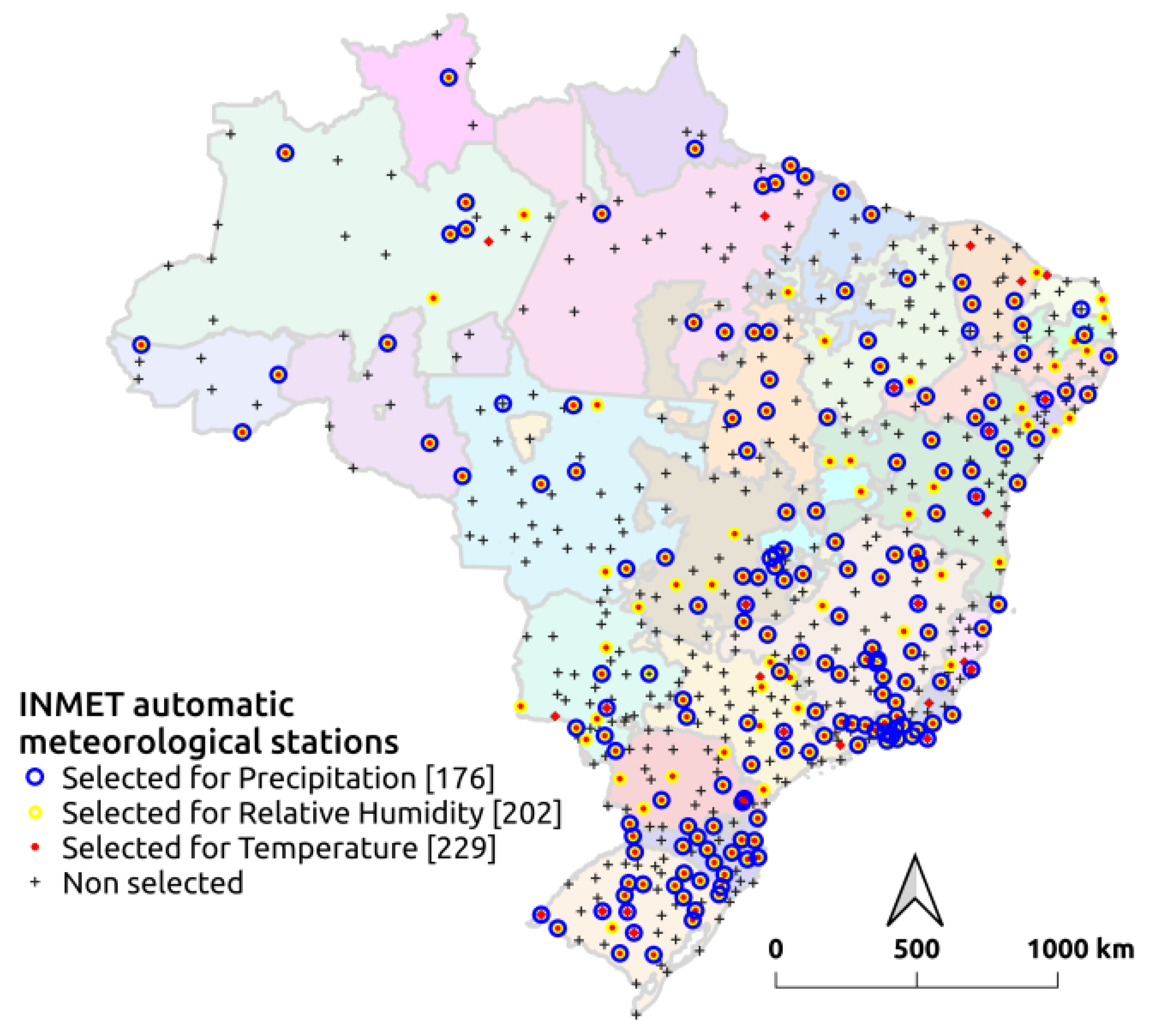
2.1.3. Meteorological Data
2.2. Data Analysis
2.2.1. Population Exposure to Environmental Factors
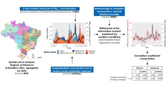
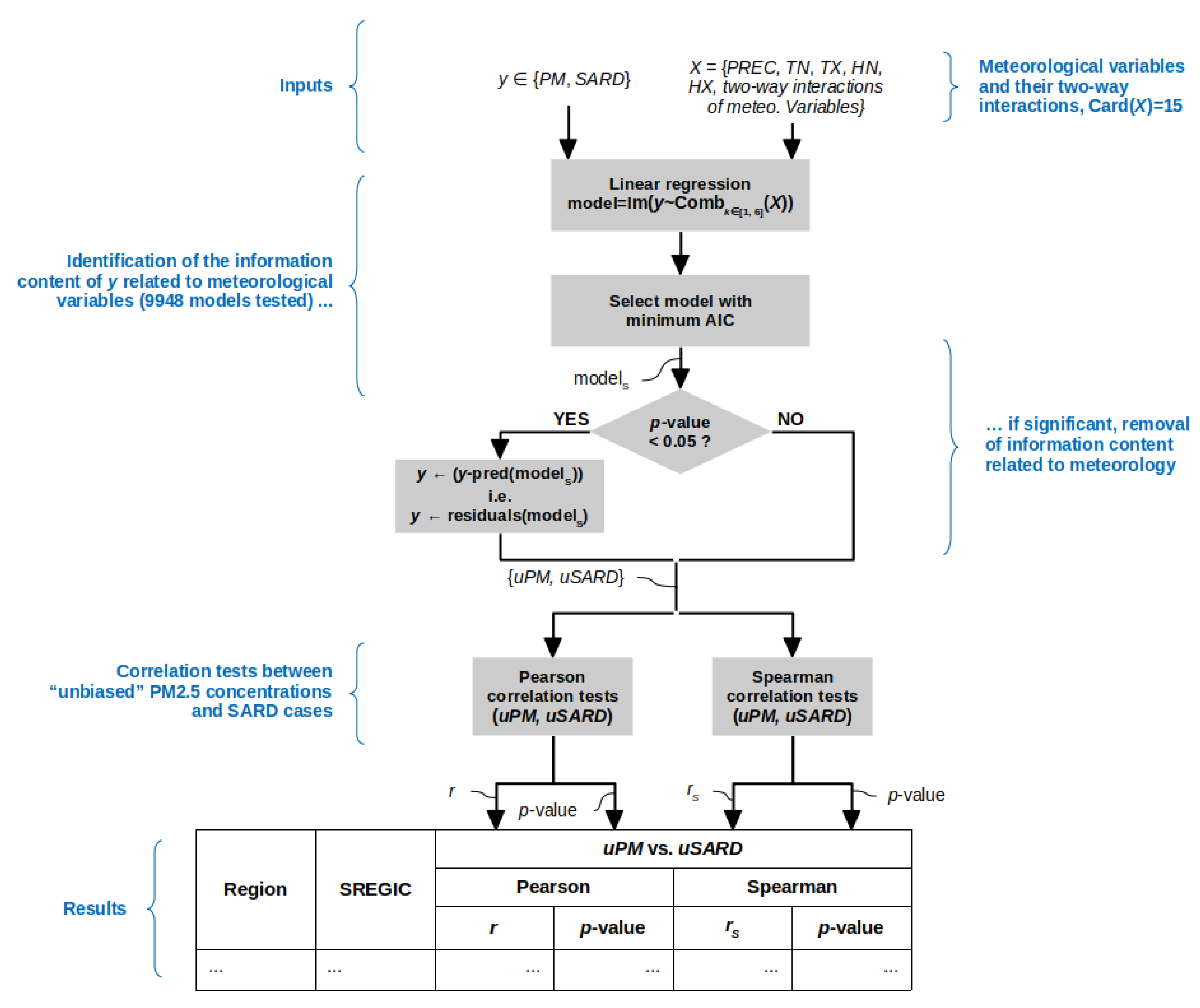
2.2.2. Correlation between PM Concentrations and SARD Cases
3. Results
3.1. Characterization of the Exposure to Environmental Factors
3.2. Spatial Distribution of SARD Cases
3.3. SpatialPM Distribution
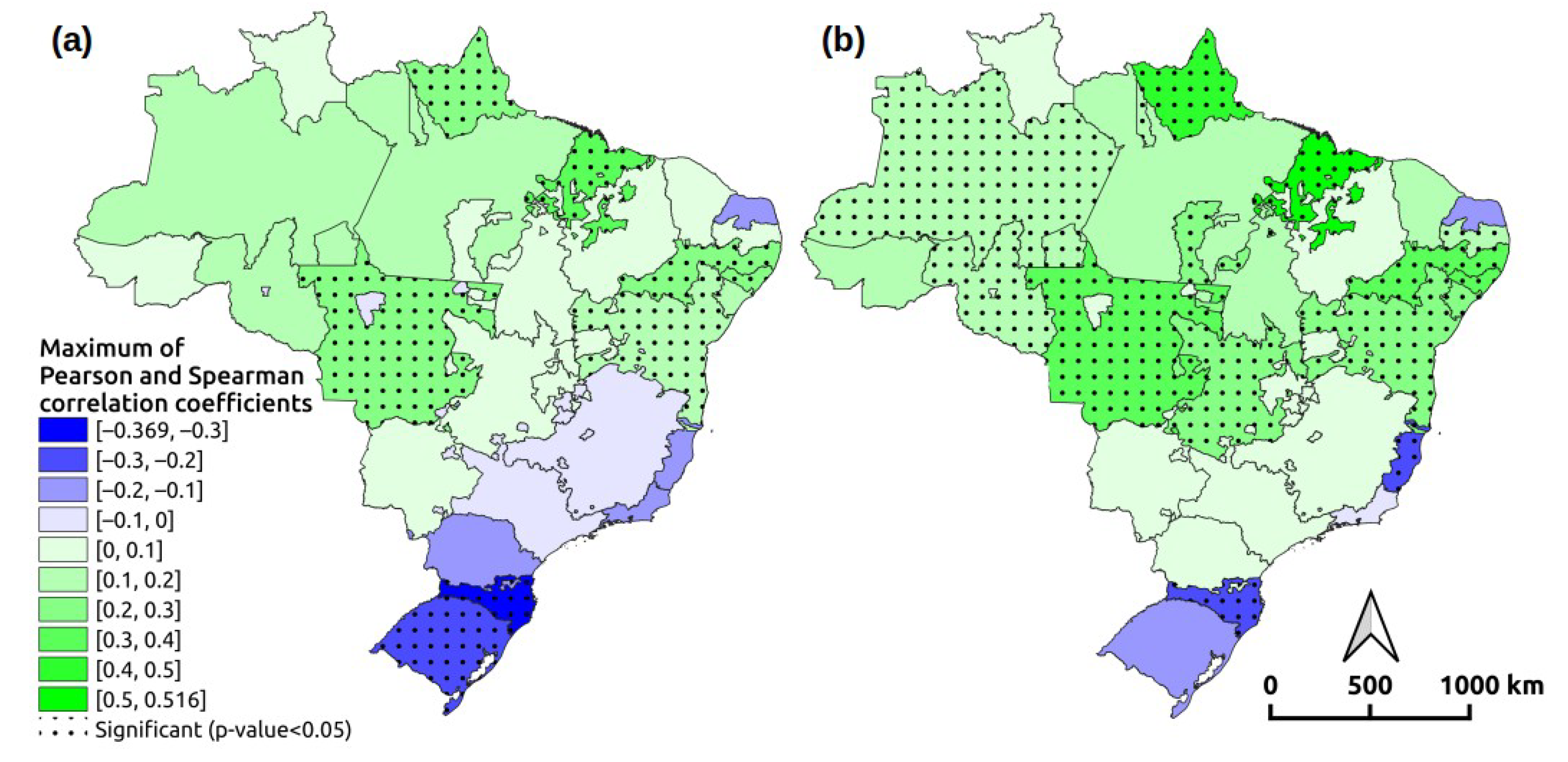
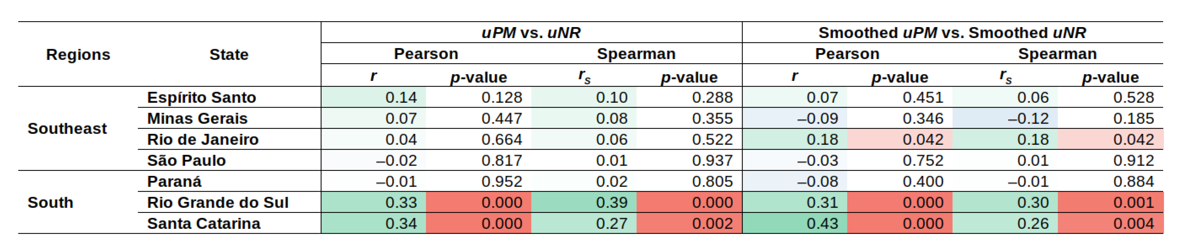
3.4. PM Concentration and SARD Case Correlations
3.5. An Early Warning System
4. Discussion
4.1. General Approach
4.2. Early Warning System Feasibility
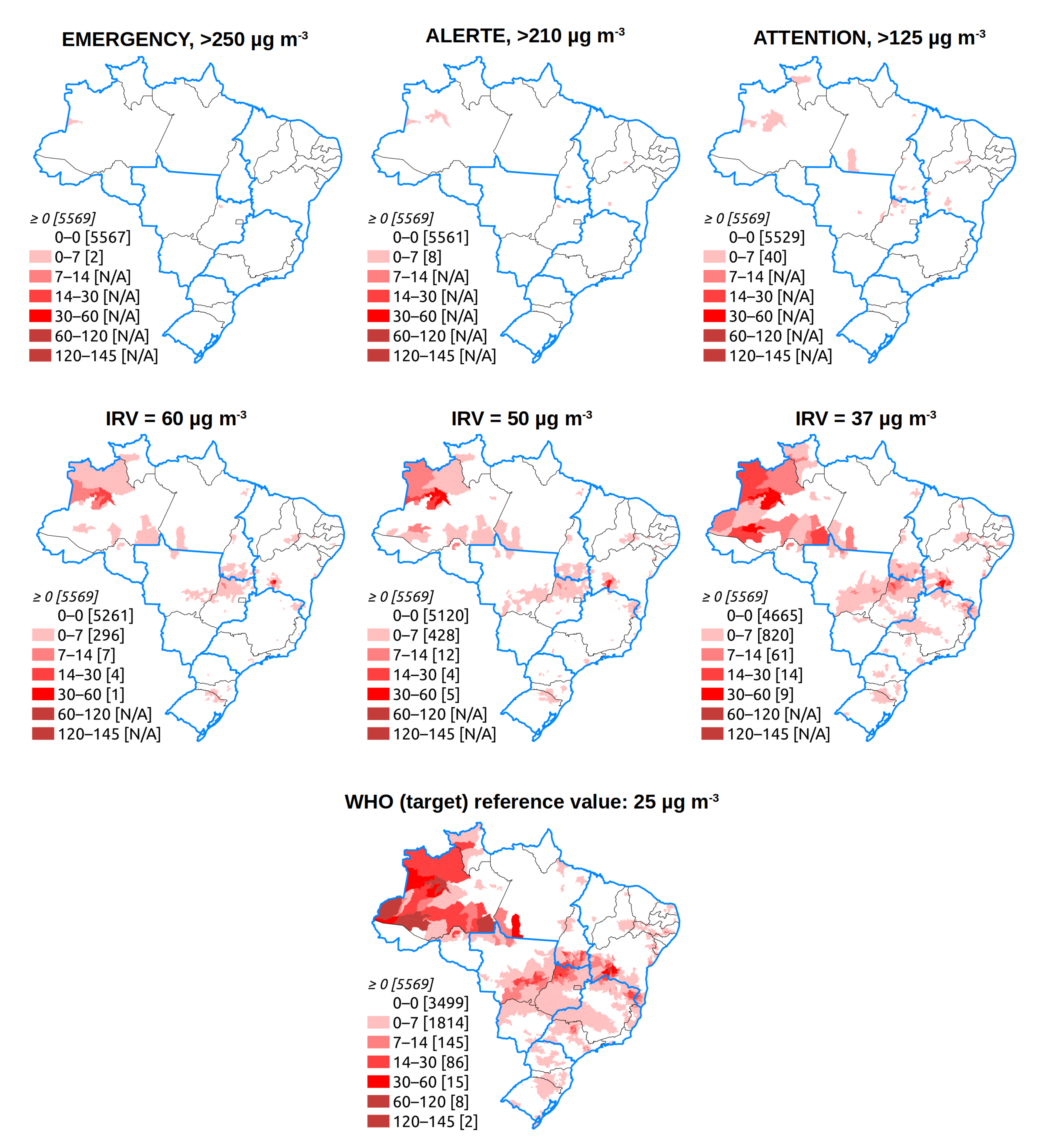
4.3. Alert Thresholds
5. Conclusions
Author Contributions
Funding
Acknowledgments
Conflicts of Interest
Abbreviations
| AIC | Akaike information criterion |
| AOD | Aerosol Optical Depth |
| CAMS | Copernicus Atmosphere Monitoring Service |
| CONAMA | Conselho Nacional de Meio Ambiente |
| ECMWF | European Centre for Medium-Range Weather Forecasts |
| EMAp | Escola de Matemática Aplicada |
| ESA | European Space Agency |
| EUMETSAT | European Organisation for the Exploitation of Meteorological Satellites |
| FGV | Fundação Getulio Vargas |
| Fiocruz | Fundação Oswaldo Cruz |
| FTP | File Transfer Protocol |
| GMAO | Global Monitoring and Assimilation Service |
| HN | minimum relative humidity |
| HX | maximum relative humidity |
| IBAMA | Instituto Brasileiro do meio ambiente e dos recursos naturais renováveis |
| IBGE | Instituto Brasileiro de Geografia e Estatistica |
| IFS | Integrated Forecasting System |
| INMET | Instituto nacional de meteorologia |
| INPE | Instituto Nacional de Pesquisa Espacial |
| MODIS | Moderate Resolution Imaging Radiospectrometer |
| NASA | National Aeronautics and Space Administration |
| NRT | Near Real Time |
| PM | Particulate Matter |
| PMAp | Polar Multi-sensor Aerosol product |
| PREC | precipitation |
| PROCC | Programa de computação científica |
| RSV | Respiratory syncytial virus |
| REGIC | Regiões de Influência das Cidades |
| SREGIC | Statewide REGIC |
| SARD | Severe Acute Respiratory Diseases |
| SARS | Severe Acute Respiratory Syndromes |
| SINAN | Sistema de Informação de Agravos de Notificação |
| SOA | Secondary Organic Aerosol |
| TN | minimum temperature |
| TX | maximum temperature |
| UTC | Coordinated Universal Time |
| WHO | World Health Organization |
Appendix A. Data Sources and Description

| Data | Spatial Resolution/ Spatial Unit | Source | Type of Access (File Format) | Question Addressed in the Study |
|---|---|---|---|---|
| PM concentration reanalyses | ∼80 km | CAMS reanalyses, Copernicus Atmosphere Data Store https://ads.atmosphere.copernicus.eu/#!/home | HTTPS (GRIB or NETCDF) | Description of the past PM concentration distribution, in space and time |
| Archived PM concentration forecasts (every 3 h) | ∼40 km | CAMS near real-time database: https://apps.ecmwf.int/datasets/data/cams-nrealtime/levtype=sfc/ | ECMWF API (GRIB or NETCDF) | Feasibility study of an early warning system; simulation of alert threshold definition |
| PM hourly concentration forecasts up to 5 days after the current day | ∼40 km | CAMS Global forecast data https://confluence.ecmwf.int/display/CKB/FTP+access+to+CAMS+global+data | FTP (GRIB) | Proposition for PM concentration indicators to be included in an early warning system (Appendix F) |
| States of Brazil | State | brazilmaps R package | (R object) | Cartography of administrative units of Brazil |
| Municipalities of Brazil (Municípios) | Municipalities | brazilmaps R package | (R object) | Simulation of alert threshold definition |
| 2019 population estimate in Brazil | State | brazilmaps R package | (R object) | SARD annual incidence |
| REGIC | REGIC | IBGE: https://www.ibge.gov.br/geociencias/cartas-e-mapas/redes-geograficas/15798-regioes-de-influencia-das-cidades.html?edicao=27334&t=downloads | HTTP (ESRI ShapeFile) | Exposure to environmental factors |
| SARD | State | InfoGripe database http://info.gripe.fiocruz.br/; https://gitlab.procc.fiocruz.br/mave/repo/tree/master/Dados/InfoGripe | HTTP (text .CSV) | Epidemiological situation related to SARD in Brazil |
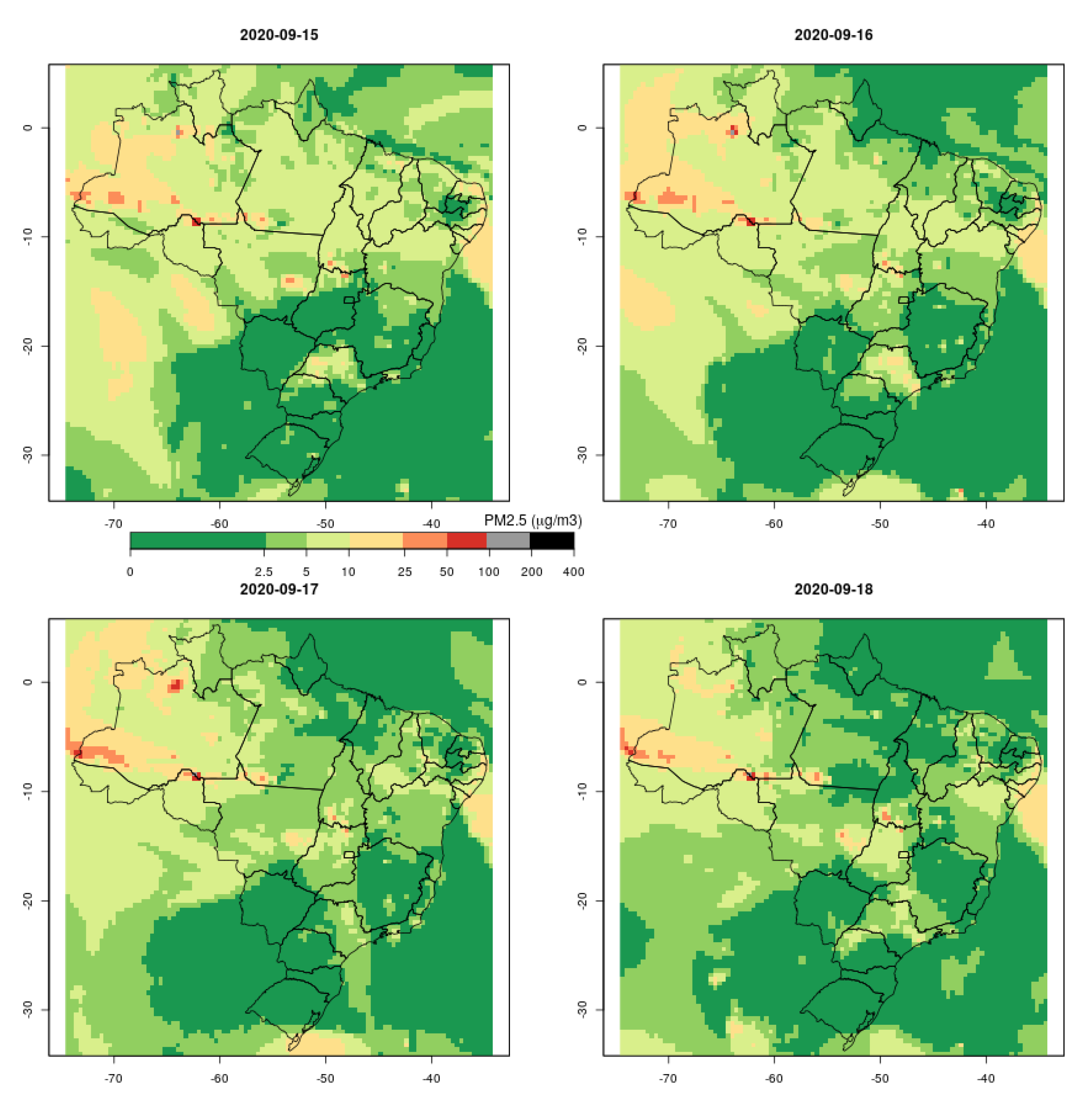
Appendix B. Examples of PM2.5 Concentration Forecasts Obtained from CAMS NRT on Which an Early Warning System Could Be Based


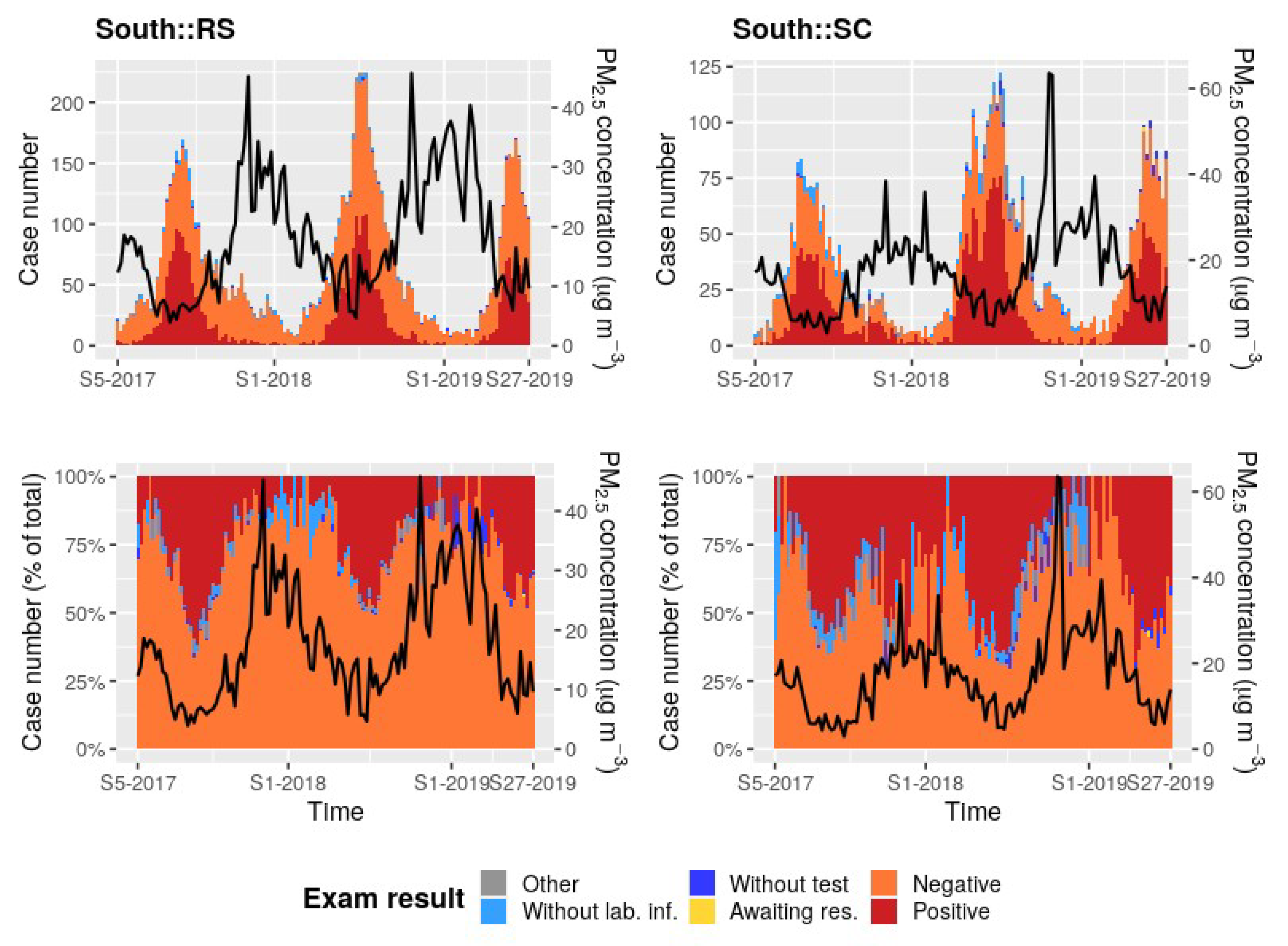
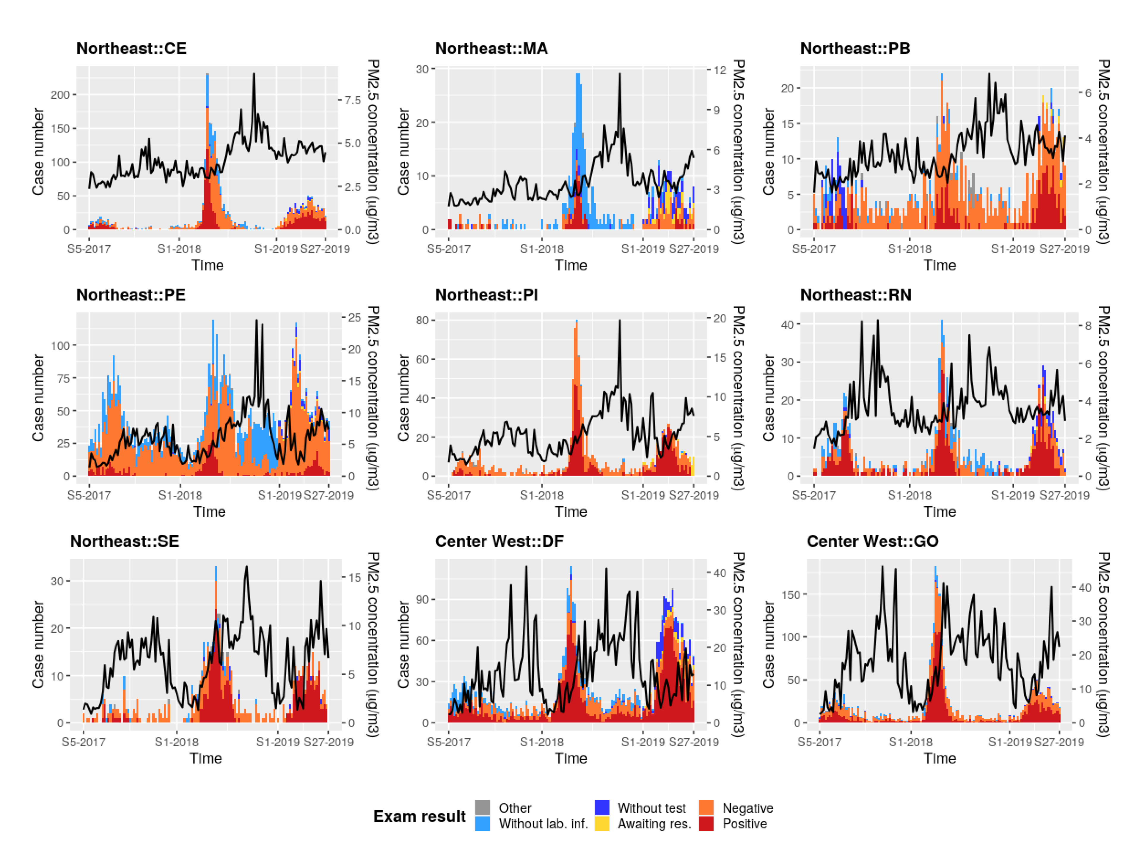
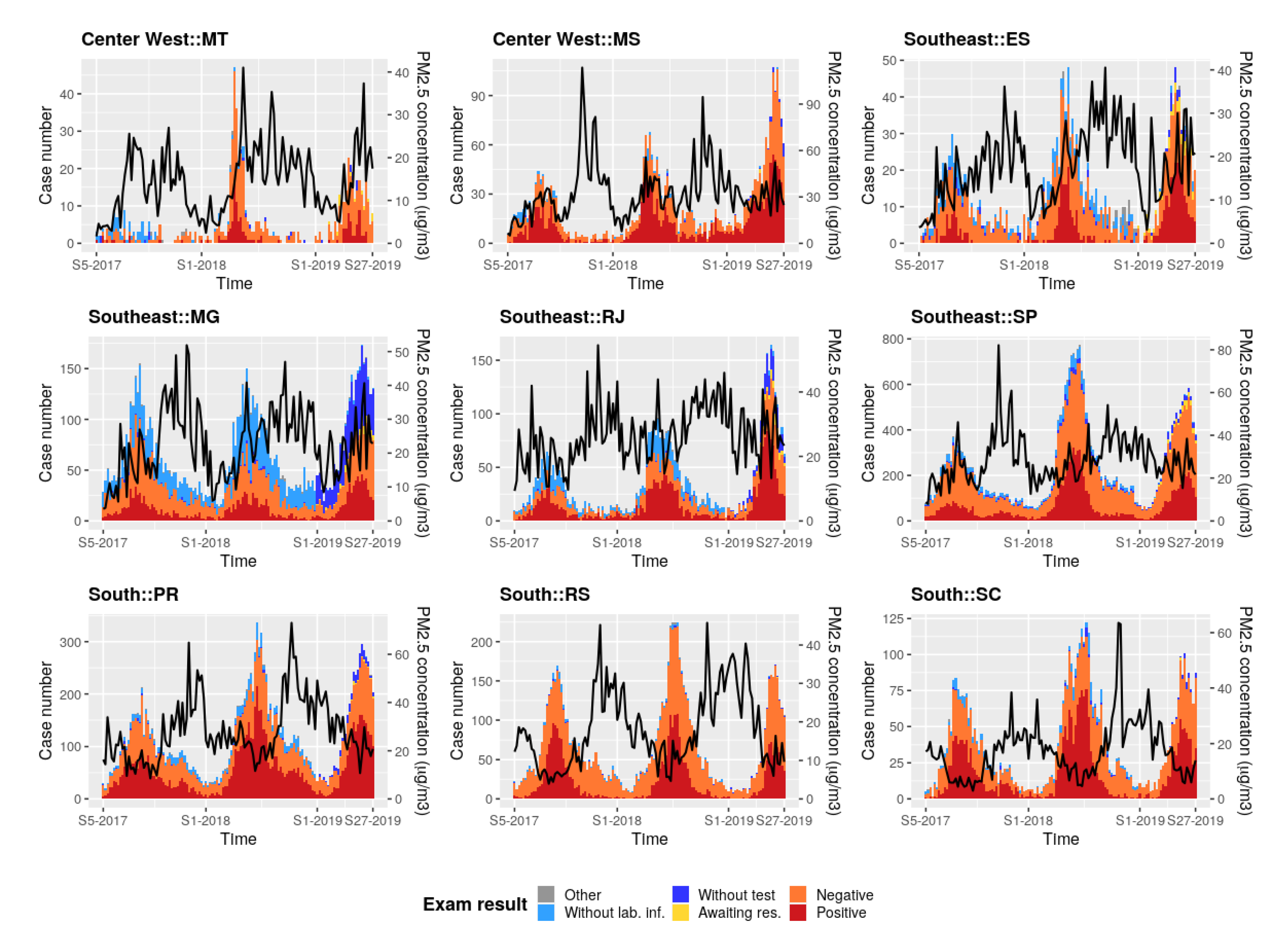
Appendix C. PM2.5 Concentration Forecasts and Weekly Case Number of SARD


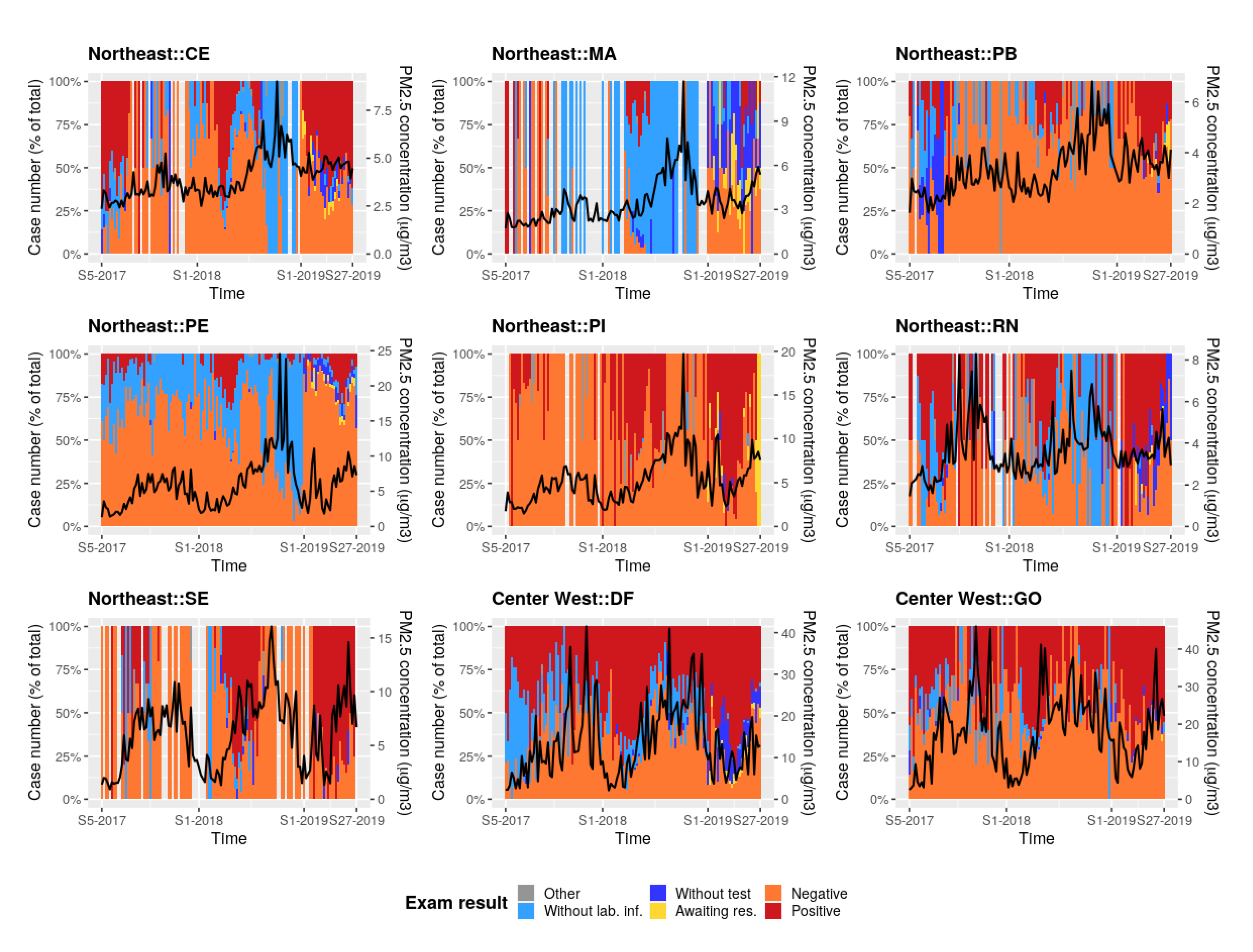
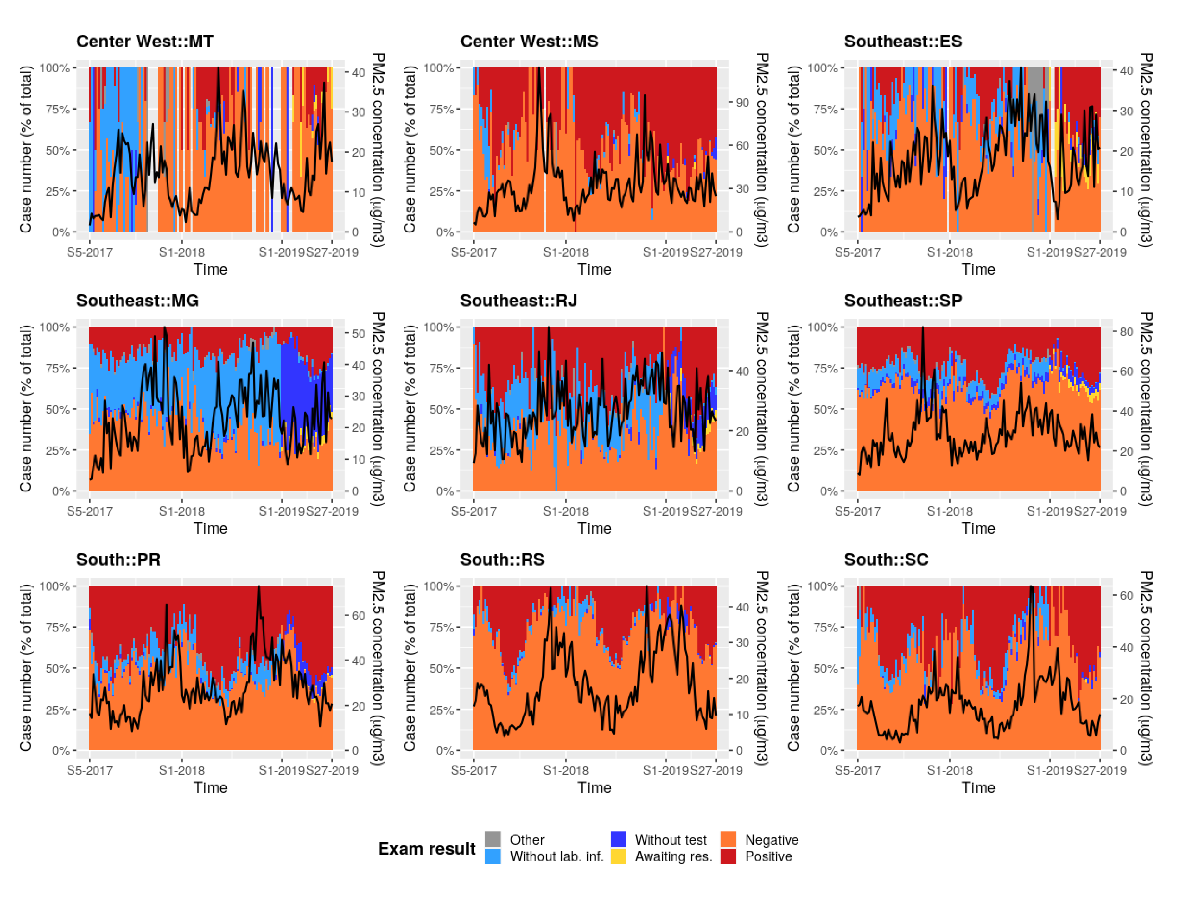
Appendix D. PM2.5 Concentration Forecasts and Weekly Case Number of SARD (in %)


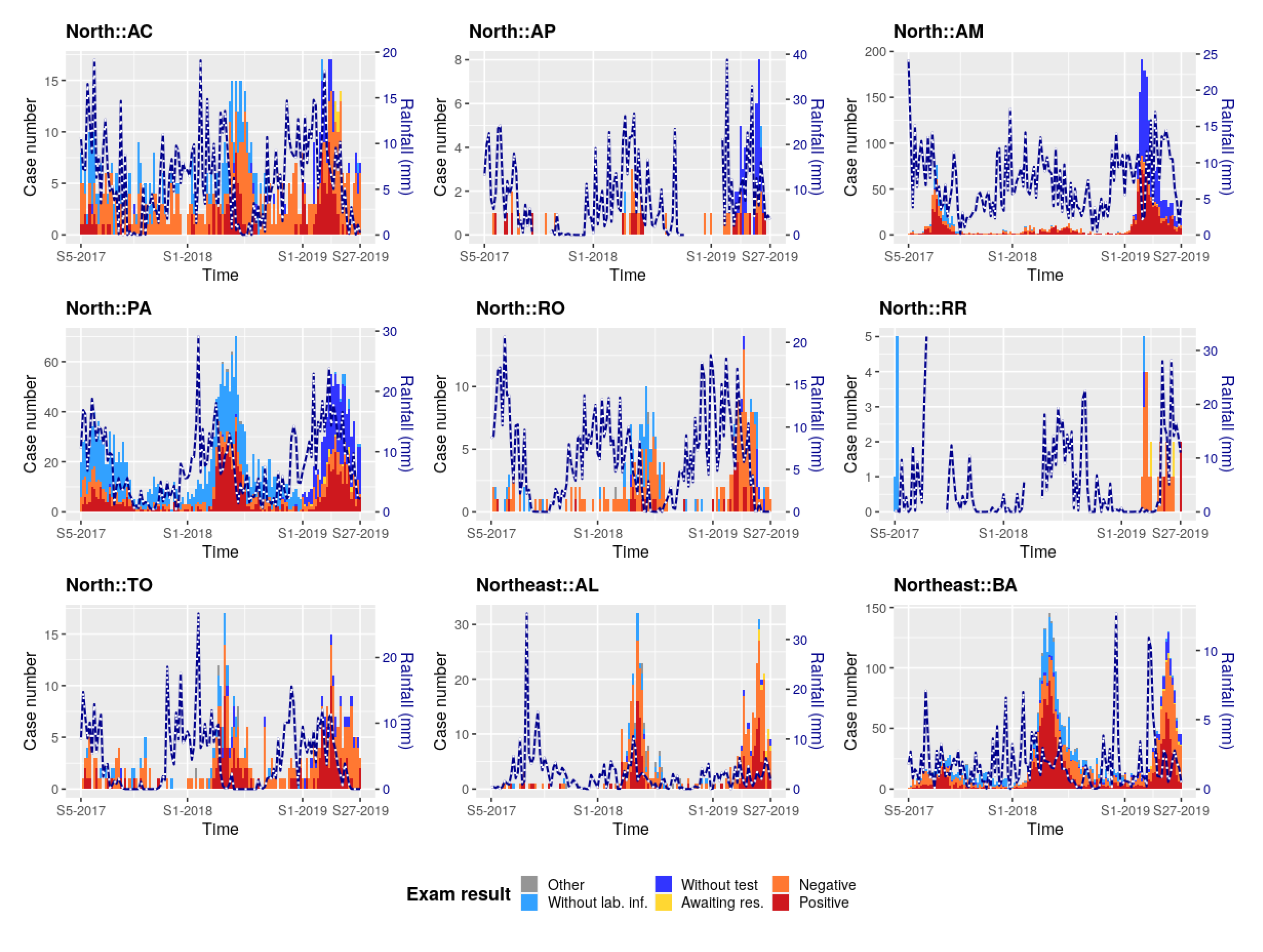
Appendix E. Rainfall and Weekly Case Number of SARD


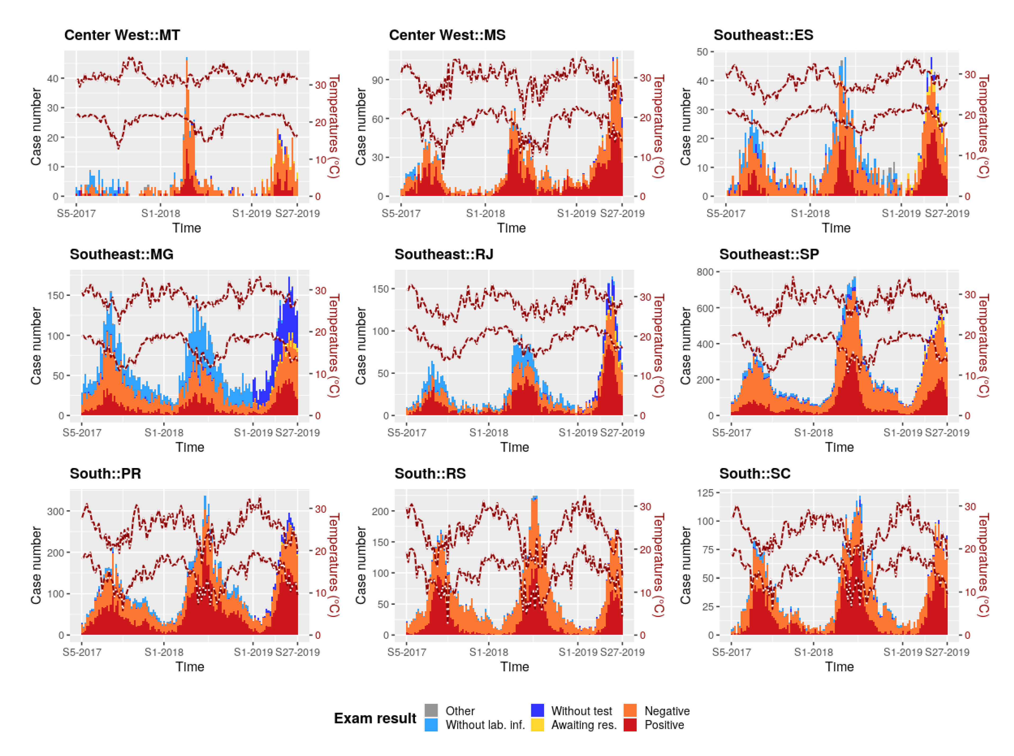
Appendix F. Temperature and Weekly Case Number of SARD


Appendix G. Relative Humidity and Weekly Case Number of SARD


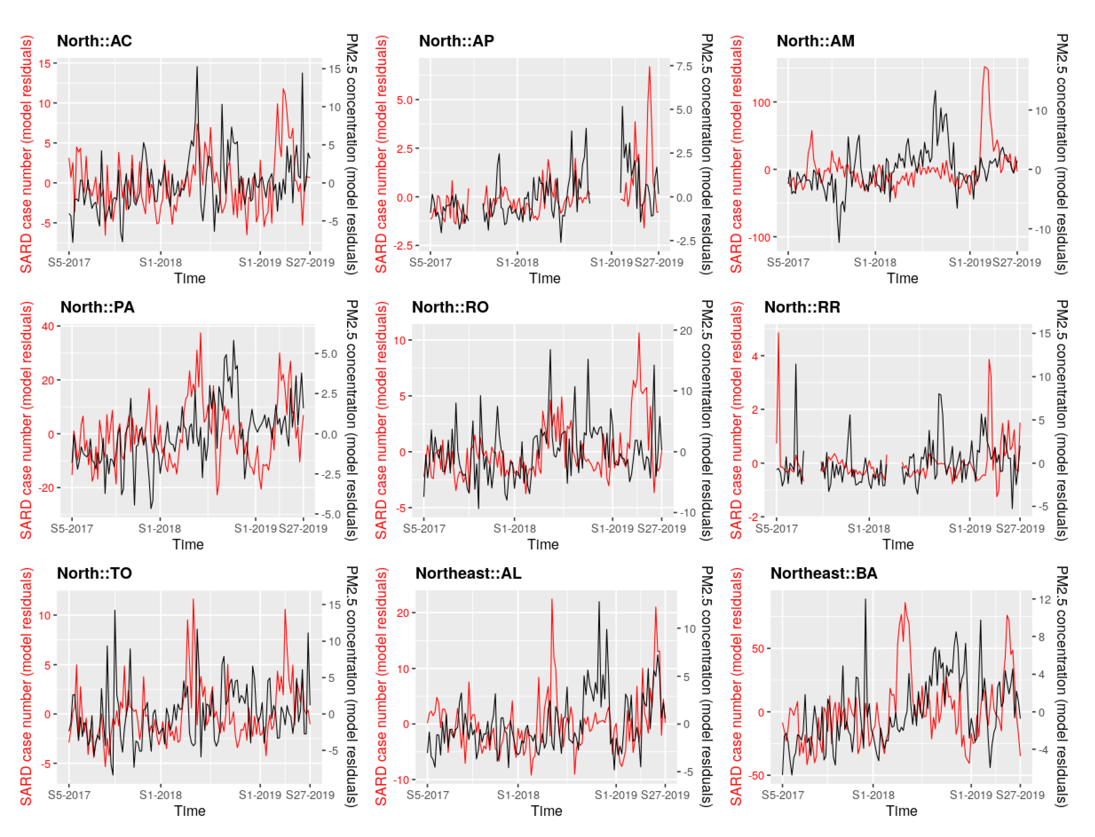
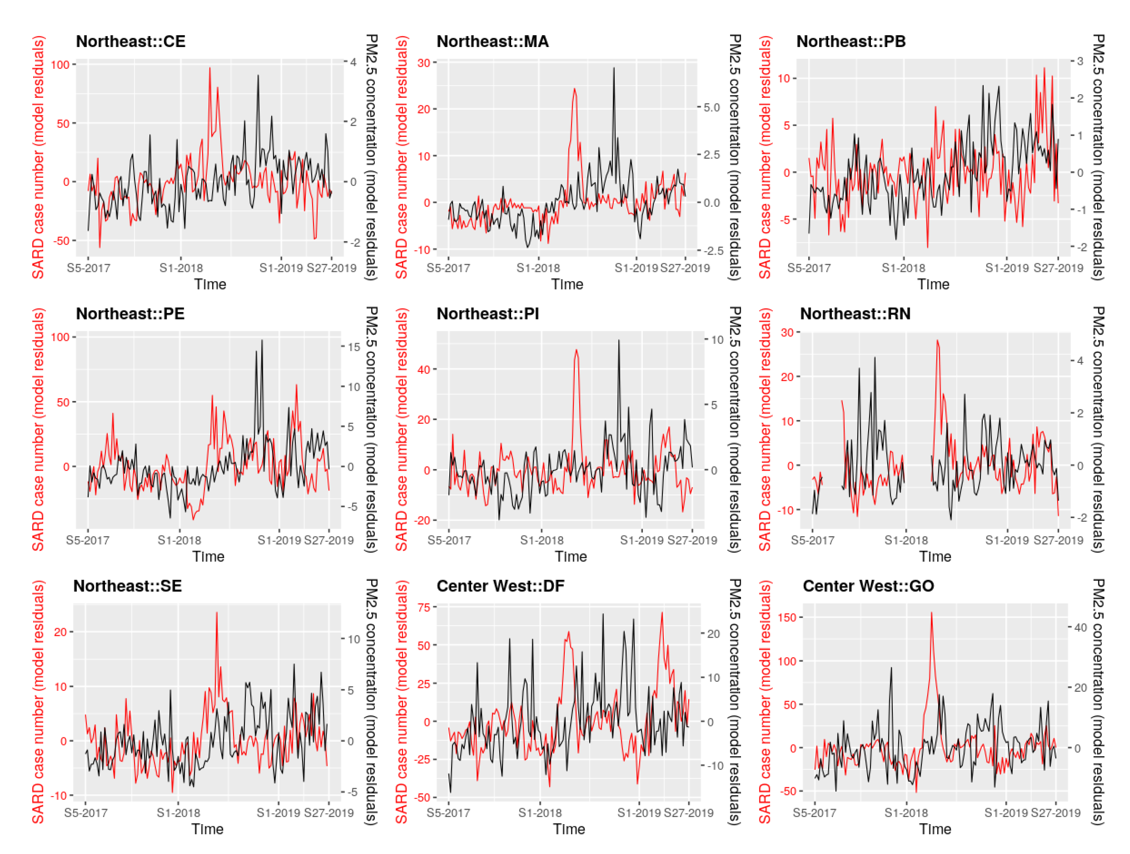
Appendix H. Residuals of the Multivariate Linear Regression Models for PM2.5 Concentrations and Case Number of SARD


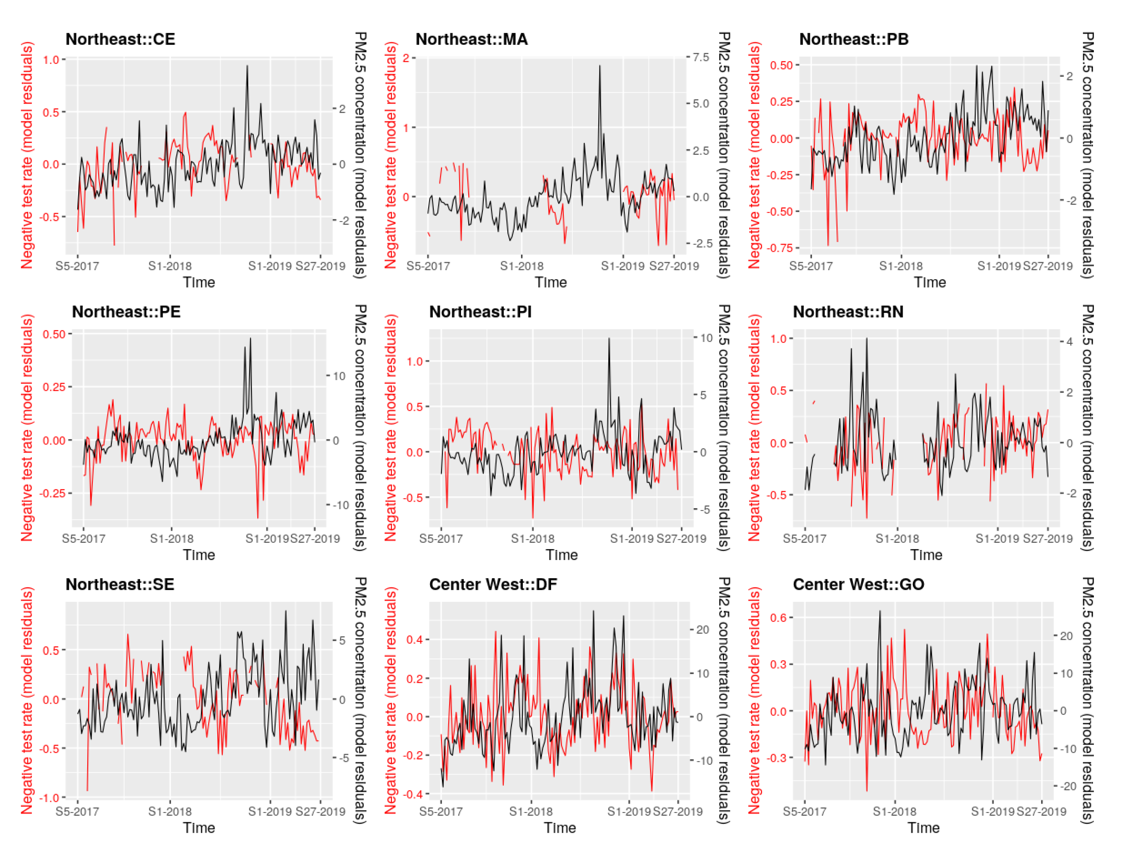
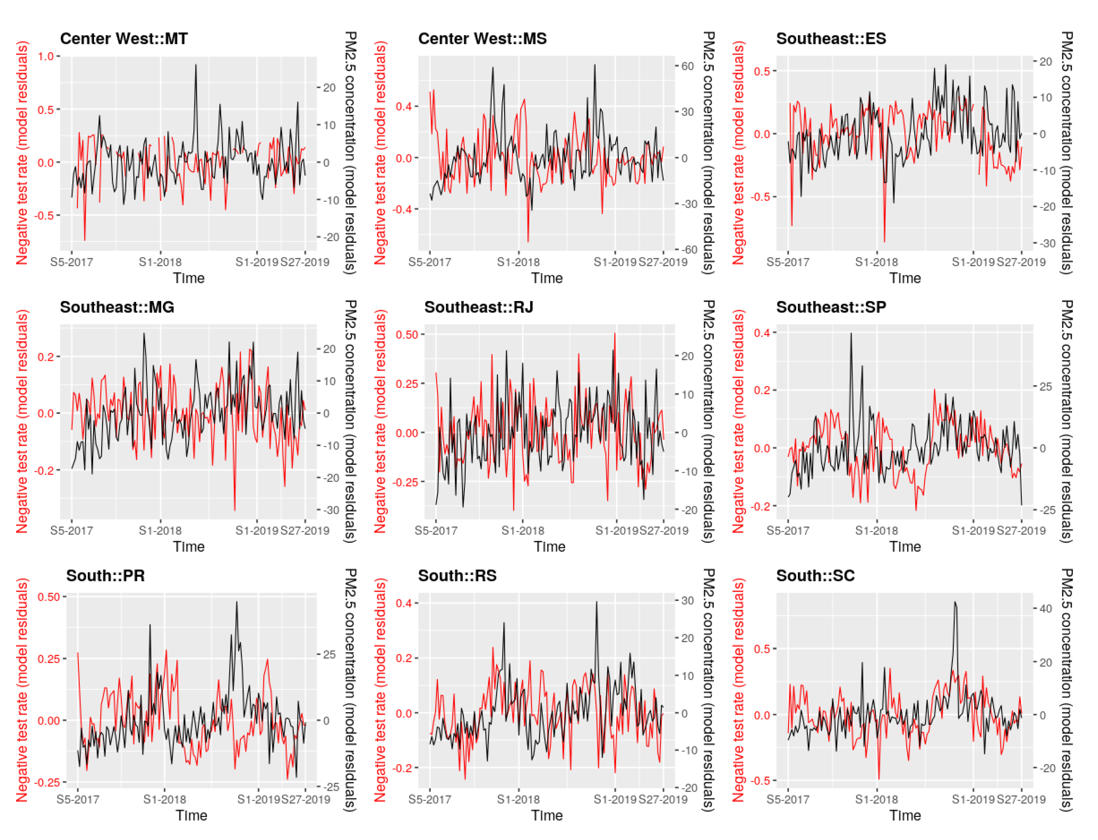
Appendix I. Residuals of the Multivariate Linear Regression Models for PM2.5 Concentrations and SARD Negative Test Rate


References
- Loomis, Y.; Lauby-Secretan, B.; El Ghissassi, F.; Bouvard, V.; Benbrahim-Tallaa, L.; Guha, N.; Baan, R.; Mattock, H.; Straif, K. on behalf of the International Agency for Research on Cancer Monograph Working Group IARC. The carcinogenicity of outdoor air pollution. Lancet 2013, 14, 1262–1263. [Google Scholar] [CrossRef]
- Health Effects Institute (HEI). State of Global Air 2019; Special Report; Health Effects Institute: Boston, MA, USA, 2019; Available online: https://www.stateofglobalair.org/sites/default/files/soga_2019_report.pdf (accessed on 9 November 2020).
- Rao, X.; Patel, P.; Puett, R.; Rajagopalan, S. Air pollution as a risk factor for type 2 diabetes. Toxicilogical Sci. 2015, 143, 231–241. [Google Scholar] [CrossRef] [PubMed] [Green Version]
- IBGE. IBGE Divulga as Estimativas da População dos Municípios para 2019. 2019. Available online: https://agenciadenoticias.ibge.gov.br/agencia-sala-de-imprensa/2013-agencia-de-noticias/releases/25278-ibge-divulga-as-estimativas-da-populacao-dos-municipios-para-2019 (accessed on 9 November 2020).
- Andreão, W.L.; Pinto, J.A.; Pedruzzi, R.; Kumar, P.; Albuquerque, T.T.A. Quantifying the impact of particle matter on mortality and hospitalizations in four Brazilian metropolitan areas. J. Environ. Manag. 2020, 270, 110840. [Google Scholar] [CrossRef] [PubMed]
- Reddington, C.L.; Butt, E.W.; Ridley, D.A.; Artaxo, P.; Morgan, W.T.; Coe, H.; Spracklen, D.V. Air quality and human health improvements from reductions in deforestation-related fire in Brazil. Nat. Geosci. 2015, 8, 768–771. [Google Scholar] [CrossRef] [Green Version]
- World Health Organization (WHO). WHO Air Quality Guidelines for Particulate Matter, Ozone, Nitrogen Dioxide and Sulfur Dioxide—Global Update 2005—Summary of Risk Assessment. 2005. Available online: https://apps.who.int/iris/handle/10665/69477 (accessed on 9 November 2020).
- Alves, N.O.; Vessoni, A.T.; Quinet, A.; Fortunato, R.S.; Kajitani, G.S.; Peixoto, M.S.; de Souza Hacon, S.; Artaxo, P.; Saldiva, P.; Menck, C.F.M.; et al. Biomass burning in the Amazon region causes DNA damage and cell death in human lung cells. Sci. Rep. 2017, 7, 10937. [Google Scholar] [CrossRef]
- Artaxo, P. Physical and chemical properties of aerosols in the wet and dry seasons in Rondônia, Amazonia. J. Geophys. Res. 2002, 107, LBA 49-1–LBA 49-14. [Google Scholar] [CrossRef]
- do Carmo, C.N.; Hacon, S.; Longo, K.M.; Freitas, S.; Ignotti, E.; Ponce de Leon, A.; Artaxo, P. Associação entre material particulado de queimadas e doenças respiratórias na região sul da Amazônia brasileira. Rev. Panam Salud Publica 2010, 27, 10–16. [Google Scholar] [CrossRef] [Green Version]
- Jacobson, L.S.V.; Hacon, S.S.; Castro, H.A.; Ignotti, E.; Artaxo, P.; Ponce de Leon, A.C.M. Association between fine particulate matter and the peak expiratory flow of schoolchildren in the Brazilian subequatorial Amazon: A panel study. Environ. Res. 2012, 117, 27–35. [Google Scholar] [CrossRef]
- Aragão, L.E.O.C.; Anderson, L.O.; Fonseca, M.G.; Rosan, T.M.; Vedovato, L.B.; Wagner, F.H.; Silva, C.V.; Junior, C.H.S.; Arai, E.; Aguiar, A.P. 21st Century drought-related fires counteract the decline of Amazon deforestation carbon emissions. Nat. Commun. 2018, 9, 536. [Google Scholar] [CrossRef]
- Aragão, L.E.O.C.; Silva Junior, C.H.L.; Anderson, L.O. Brazil’s Challenge to Restrain Deforestation and Fires in the Amazon during COVID-19 Pandemic in 2020: Environmental, Social Implications and Their Governance; Technical Note; Instituto Nacional de Pesquisas Espaciais (INPE): São José dos Campos, Brazil, 2020; 34p. [Google Scholar] [CrossRef]
- Observatório de Clima e Saúde (ICIC/Fiocruz). Covid-19 e Queimadas na Amazônia Legal e no Pantanal: Aspectos Cumulativos e Vulnerabilidades. Technical Note. 2020. Available online: https://www.icict.fiocruz.br/sites/www.icict.fiocruz.br/files/nota_queimadascovid_out2020.pdf (accessed on 13 November 2020).
- Henderson, S.B. The Covid-19 Pandemic and Wildfire Smoke: Potentially Concomitant Disasters. Am. J. Public Health 2020, 110, e1–e3. [Google Scholar] [CrossRef]
- Sedlmaier, N.; Hoppenheidt, K.; Krist, H.; Lehmann, S.; Lang, H. Generation of avian influenza virus (AIV) contaminated fecal fine particulate matter (PM): Genome and infectivity detection and calculation of immission. Vet. Microbiol. 2009, 139, 156–164. [Google Scholar] [CrossRef] [PubMed] [Green Version]
- Després, V.R.; Huffman, J.A.; Burrows, S.M.; Hoose, C.; Safatov, A.S.; Buryak, G.; Fröhlich-Nowoisky, J.; Elbert, W.; Andreae, M.O.; Pöschl, U.; et al. Primary biological aerosol particles in the atmosphere: A review. Tellus B Chem. Phys. Meteorol. 2012, 64, 15598. [Google Scholar] [CrossRef] [Green Version]
- Setti, L.; Passarini, F. Relazione Circa l’Effetto Dell’inquinamento da Particolato Atmosferico e la Diffusione di Virus Nella Popolazione. Actu-Environnement Website, 2020. Available online: https://www.actu-environnement.com/media/pdf/news-35178-covid-19.pdf (accessed on 13 October 2020).
- Gaddi, A.V.; Capello, F. Particulate Does Matter: Is Covid-19 Another Air Pollution Related Disease? Preprint 2020. Available online: https://doi.org/10.13140/RG.2.2.22283.85286/2 (accessed on 11 December 2020).
- Han, Y.; Lam, J.C.K.; Li, V.O.K.; Guo, P.; Zhang, Q.; Wang, A.; Crowcroft, J.; Wang, S.; Fu, J.; Gilani, Z.; et al. The effects of outdoor air pollution concentrations and lockdowns on Covid-19 infections in Wuhan and other provincial capitals in China. Preprint 2020. Available online: https://doi.org/10.20944/preprints202003.0364.v1 (accessed on 11 December 2020).
- Andrée, B.P.J. Incidence of COVID-19 and Connections with Air Pollution Exposure: Evidence from the Netherlands; Policy Research Working Paper No. 9221; World Bank: Washington, DC, USA, 2020. [Google Scholar]
- Wu, X.; Nethery, R.C.; Sabath, M.B.; Braun, D.; Dominici, F. Air pollution and COVID-19 mortality in the United States: Strengths and limitations of an ecological regression analysis. Sci. Adv. 2020, 6, eabd4049. [Google Scholar] [CrossRef] [PubMed]
- Pope, C.A., III; Burnett, R.T.; Thun, M.J.; Calle, E.E.; Krewski, D.; Ito, K.; Thurston, G.D. Lung cancer, cardiopulmonary mortality, and long-term exposure to fine particulate air pollution. JAMA 2002, 287, 1132–1141. [Google Scholar] [CrossRef] [Green Version]
- World Health Organization (WHO) Regional Office for Europe. Review of Evidence on Health Aspects of Air Pollution—REVIHAAP Project. Technical Report. 2013. Available online: https://www.euro.who.int/__data/assets/pdf_file/0004/193108/REVIHAAP-Final-technical-report-final-version.pdf (accessed on 9 November 2020).
- Vormittag, E.; Almeida, R. Avaliação da RESOLUção 491/2018 Quanto à sua Efetividade para Proteção da Saúde e Sobre os Mecanismos de Informação à Sociedade. Technical Report of the Instituto Saúde e Sustentabilidadet. 2019. Available online: https://www.saudeesustentabilidade.org.br/wp-content/uploads/2019/06/Avaliacao-491.18-rev3final.pdf (accessed on 13 October 2020).
- Siciliano, B.; Dantas, G.; da Silva, C.M.; Arbilla, G. The Updated Brazilian National Air Quality Standards: A Critical Review. J. Braz. Chem. Soc. 2020, 31, 523–535. [Google Scholar] [CrossRef]
- Lizundia-Loiola, J.; Pettinari, M.L.; Chuvieco, E. Temporal Anomalies in Burned Area Trends: Satellite Estimations of the Amazonian 2019 Fire Crisis. Remote Sens. 2020, 12, 151. [Google Scholar] [CrossRef] [Green Version]
- Chau, K.; Franklin, M.; Gauderman, W.J. Satellite-Derived PM2.5 Composition and Its Differential Effect on Children’s Lung Function. Remote Sens. 2020, 12, 1028. [Google Scholar] [CrossRef] [Green Version]
- Peláez, L.M.G.; Santos, J.M.; de Almeida Albuquerque, T.T.; Reis, N.C., Jr.; Andreão, W.L.; de Fátima, A.M. Air quality status and trends over large cities in South America. Environ. Sci. Policy 2020, 114, 422–435. [Google Scholar] [CrossRef]
- Grupo de Métodos Analíticos de Vigilância Epidemiológica (MAVE). PROCC/Fiocruz e EMap/FGV, e GT-Influenza da Secretaria de Vigilância em Saúde do Ministério da Saúde. InfoGripe Website. Available online: http://info.gripe.fiocruz.br/ (accessed on 13 October 2020).
- Grupo de Métodos Analíticos de Vigilância Epidemiológica (MAVE). PROCC/Fiocruz e EMap/FGV, e GT-Influenza da Secretaria de Vigilância em Saúde do Ministério da Saúde. InfoGripe Online Repository. Available online: https://gitlab.procc.fiocruz.br/mave/repo/-/tree/master/Dados/InfoGripe (accessed on 13 October 2020).
- Rémy, S.; Kipling, Z.; Flemming, J.; Boucher, O.; Nabat, P.; Michou, M.; Bozzo, A.; Ades, M.; Huijnen, V.; Benedetti, A.; et al. Description and evaluation of the tropospheric aerosol scheme in the European Centre for Medium-Range Weather Forecasts (ECMWF) Integrated Forecasting System (IFS-AER, cycle 45R1). Geosci. Model Dev. 2019, 12, 4627–4659. [Google Scholar] [CrossRef] [Green Version]
- Inness, A.; Ades, M.; Agustí-Panareda, A.; Barré, J.; Benedictow, A.; Blechschmidt, A.-M.; Dominguez, J.J.; Engelen, R.; Eskes, H.; Flemming, J.; et al. The CAMS reanalysis of atmospheric composition. Atmos. Chem. Phys. 2019, 19, 3515–3556. [Google Scholar] [CrossRef] [Green Version]
- Freitas, A.R.R.; Donalisio, M.R. Respiratory syncytial virus seasonality in Brazil: Implications for the immunisation policy for at-risk populations. Mem. Inst. Oswaldo Cruz 2016, 111. [Google Scholar] [CrossRef] [PubMed] [Green Version]
- Wiemken, T.L.; Mattingly, W.A.; Furmanek, S.P.; Guinn, B.E.; English, C.L.; Carrico, R.; Peyrani, P.; Ramirez, J.A. Impact of Temperature Relative Humidity and Absolute Humidity on the Incidence of Hospitalizations for Lower Respiratory Tract Infections Due to Influenza, Rhinovirus, and Respiratory Syncytial Virus: Results from Community-Acquired Pneumonia Organization (CAPO) International Cohort Study. Univ. Louisville J. Respir. Infect. 2017, 1, 7. [Google Scholar] [CrossRef]
- Basart, S.; Benedictow, A.; Bennouna, Y.; Blechschmidt, A.-M.; Chabrillat, S.; Christophe, Y.; Cuevas, E.; Eskes, H.J.; Hansen, K.M.; Jorba, O. Upgrade Verification Note for the CAMS Real-Time Global Atmospheric Composition Service: Evaluation of the E-suite for the CAMS Upgrade of July 2019; Copernicus Atmosphere Monitoring Service (CAMS) Report; ECMWF—Shinfield Park: Reading, UK, 2019; Available online: https://doi.org/10.24380/fcwq-yp50 (accessed on 11 December 2020).


Publisher’s Note: MDPI stays neutral with regard to jurisdictional claims in published maps and institutional affiliations. |
© 2020 by the authors. Licensee MDPI, Basel, Switzerland. This article is an open access article distributed under the terms and conditions of the Creative Commons Attribution (CC BY) license (http://creativecommons.org/licenses/by/4.0/).
Share and Cite
Roux, E.; Ignotti, E.; Bègue, N.; Bencherif, H.; Catry, T.; Dessay, N.; Gracie, R.; Gurgel, H.; de Sousa Hacon, S.; de A. F. M. Magalhães, M.; et al. Toward an Early Warning System for Health Issues Related to Particulate Matter Exposure in Brazil: The Feasibility of Using Global PM2.5 Concentration Forecast Products. Remote Sens. 2020, 12, 4074. https://doi.org/10.3390/rs12244074
Roux E, Ignotti E, Bègue N, Bencherif H, Catry T, Dessay N, Gracie R, Gurgel H, de Sousa Hacon S, de A. F. M. Magalhães M, et al. Toward an Early Warning System for Health Issues Related to Particulate Matter Exposure in Brazil: The Feasibility of Using Global PM2.5 Concentration Forecast Products. Remote Sensing. 2020; 12(24):4074. https://doi.org/10.3390/rs12244074
Chicago/Turabian StyleRoux, Emmanuel, Eliane Ignotti, Nelson Bègue, Hassan Bencherif, Thibault Catry, Nadine Dessay, Renata Gracie, Helen Gurgel, Sandra de Sousa Hacon, Mônica de A. F. M. Magalhães, and et al. 2020. "Toward an Early Warning System for Health Issues Related to Particulate Matter Exposure in Brazil: The Feasibility of Using Global PM2.5 Concentration Forecast Products" Remote Sensing 12, no. 24: 4074. https://doi.org/10.3390/rs12244074