Article

Assessment of Spatio-Temporal Landscape Changes from VHR Images in Three Different Permafrost Areas in the Western Russian Arctic

1
Department of Geography, West University of Timişoara, 300223 Timişoara, Romania
2
Helmholtz Centre for Polar & Marine Research, Alfred Wegener Institute, 27570 Bremerhaven, Germany
3
Institute of Coastal Research, Helmholtz-Zentrum Geesthacht, 21502 Geesthacht, Germany
4
Max Planck Institute for Meteorology, 20146 Hamburg, Germany
*
Author to whom correspondence should be addressed.
Remote Sens. 2020, 12(23), 3999; https://doi.org/10.3390/rs12233999
Submission received: 1 November 2020 / Revised: 29 November 2020 / Accepted: 3 December 2020 / Published: 7 December 2020
(This article belongs to the Special Issue Environmental Mapping Using Remote Sensing)

Abstract

:
Our study highlights the usefulness of very high resolution (VHR) images to detect various types of disturbances over permafrost areas using three example regions in different permafrost zones. The study focuses on detecting subtle changes in land cover classes, thermokarst water bodies, river dynamics, retrogressive thaw slumps (RTS) and infrastructure in the Yamal Peninsula, Urengoy and Pechora regions. Very high-resolution optical imagery (sub-meter) derived from WorldView, QuickBird and GeoEye in conjunction with declassified Corona images were involved in the analyses. The comparison of very high-resolution images acquired in 2003/2004 and 2016/2017 indicates a pronounced increase in the extent of tundra and a slight increase of land covered by water. The number of water bodies increased in all three regions, especially in discontinuous permafrost, where 14.86% of new lakes and ponds were initiated between 2003 and 2017. The analysis of the evolution of two river channels in Yamal and Urengoy indicates the dominance of erosion during the last two decades. An increase of both rivers’ lengths and a significant widening of the river channels were also observed. The number and total surface of RTS in the Yamal Peninsula strongly increased between 2004 and 2016. A mean annual headwall retreat rate of 1.86 m/year was calculated. Extensive networks of infrastructure occurred in the Yamal Peninsula in the last two decades, stimulating the initiation of new thermokarst features. The significant warming and seasonal variations of the hydrologic cycle, in particular, increased snow water equivalent acted in favor of deepening of the active layer; thus, an increasing number of thermokarst lake formations.

Graphical Abstract

1. Introduction

Over the past three decades, arctic regions have experienced various changes in land cover [1] and landscape structure [2] due to the rapid increase of air temperature [3] and human development [4]. In high-latitude regions, the recent atmospheric warming trend was considerably stronger than elsewhere, with an average increase of surface air temperature of about 0.6 °C/decade over the last 30 years [3]. Arctic regions are extensively underlain by permafrost and thus very sensitive to rising air temperatures [5] since higher air temperatures mainly drive the observed enhanced degradation of permafrost [6]. Permafrost warming significantly impacts local hydrology [7], vegetation [8], topography [9], soil processes [10], infrastructure and local communities [11] and may cause climate impacts on a global scale [12]. Therefore, permafrost has been recently added as an essential climate variable by the Global Climate Observing System.
Despite northern environments being subjected to recent dramatic changes, there is still an insufficient understanding of the complex climate-permafrost-ecosystem interactions [13]. Large regions in the high latitudes of the Northern Hemisphere remain relatively understudied due to harsh environments and remoteness, leading to incomplete knowledge of the disturbances and significance of change to environmental processes. In this context, remote sensing techniques have proved to be valuable tools to analyze changing landscapes in arctic regions [1]. In the last decades, low to high-resolution satellite images, such as those from advanced very high-resolution radiometer (AVHRR) (1 km spatial resolution), moderate resolution imaging spectroradiometer (MODIS) (250 m), Landsat (30 m), advanced space-borne thermal emission and reflection radiometer (ASTER) (15 m), Sentinel (20 m), Satellite Pour l’Observation de la Terre (SPOT) (10 m), coupled with improved algorithms for image processing provide critical and detailed information on land cover changes [14], vegetation greening [15,16], the surface area of water bodies [17], retrogressive thaw slumps activity [18], fire occurrence [19], et cetera. However, in many cases, the coarse resolution of freely available remote sensing products was inappropriate to detect subtle changes in the arctic ecosystems [20]. Recent contributions revealed, for example, an underestimation in the surface area of water bodies due to inadequate spatial resolution of medium to high-resolution of satellite imagery analysis (e.g., moderate resolution imaging spectroradiometer—250 m resolution; Landsat—30 m resolution) [21]. It has been shown that the resolution of Landsat images is too coarse to detect ponds in tundra environments and might underestimate the water surface by a factor of 1.5 [22]. Concurrently, the omission of Siberian tundra ponds would mean an underestimation of carbon dioxide emissions of 35–62% [23].
However, only a small number of studies have used very high-resolution (VHR) imagery (<5 m resolution) for a more accurate mapping of Arctic coastlines [24], small water bodies [25], vegetation distribution [26], land cover classes [4] or ice-wedge degradation [27].
Since the Arctic landscapes’ responses to atmospheric warming are very heterogeneous at local scales [28], different categories of disturbances cannot be detected by coarse resolution remote sensing imagery [29]. In recent years Ikonos, Quickbird, GeoEye, WorldView, Pleiades, TerraSAR-X, Cosmo-Skymed, Planet, et cetera, and many other VHR satellites have been launched, and provide more detailed disturbance detection and analysis about Arctic features. Despite recent progress in this field, there are still enormous gaps concerning the inventories of permafrost related disturbances at very high resolution due to the high cost and limited availability of such images.
The amplified Arctic warming over the past decade was significantly stronger over Siberia compared with North America [30]. Consequently, permafrost has warmed throughout Siberia, reaching its maximum in the northwestern Siberia (at Marre Sale permafrost station in the Yamal Peninsula) where permafrost temperature increased by almost 1 °C between 2008 and 2016 [5,6]. According to recent estimates, 25–90% of near surface-permafrost will degrade into seasonally frozen ground by the end of this century [31,32], thereby releasing large amounts of greenhouse gases into the atmosphere and triggering further warming of the atmosphere [12]. However, Arctic environment responses to atmospheric warming are very heterogeneous due to disproportional warming of the mosaicked landscapes and nonlinear manifestation of different climate-induced processes [33]. As the Arctic warms, complex interactions of permafrost thawing with hydrology, topography, climate and land cover at various spatial and temporal scales occur [34].
In this research, we combine the use of very high-resolution optical imagery (sub-meter) derived from WorldView, QuickBird and GeoEye in conjunction with declassified Corona images to quantify various types of changes in land cover, thermokarst water bodies, river dynamics, retrogressive thaw slumps (RTS) and infrastructure in three sites distributed in West Siberia and northeastern European Russia (Figure 1). To establish a link between the small-scale processes and their regional climate drivers, VHR images have been compared with medium resolution European Space Agency (ESA) Permafrost climate change initiative (CCI) active layer thickness map [35]) and the climate parameters from ERA-Interim reanalysis [36]. Moreover, the results and maps from VHR images could be used as a useful resource in other applications related to ecological modeling or habitat management [25].

2. Materials and Methods
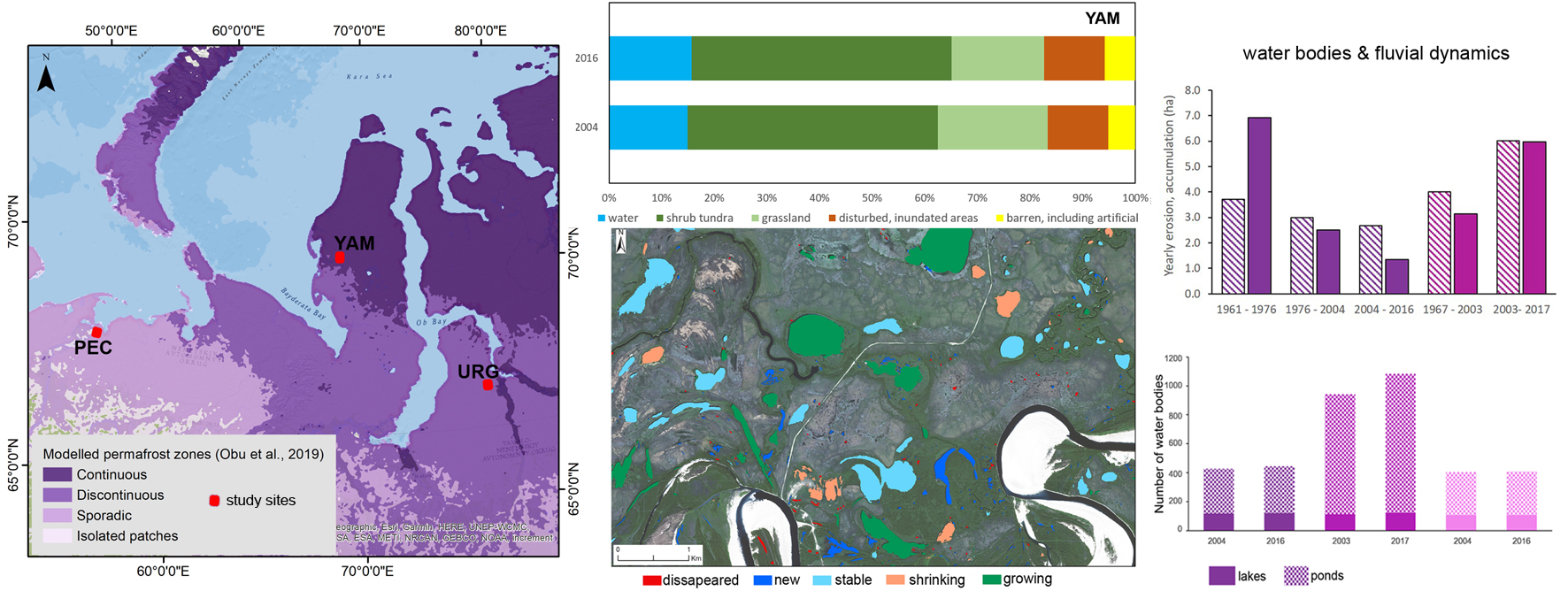
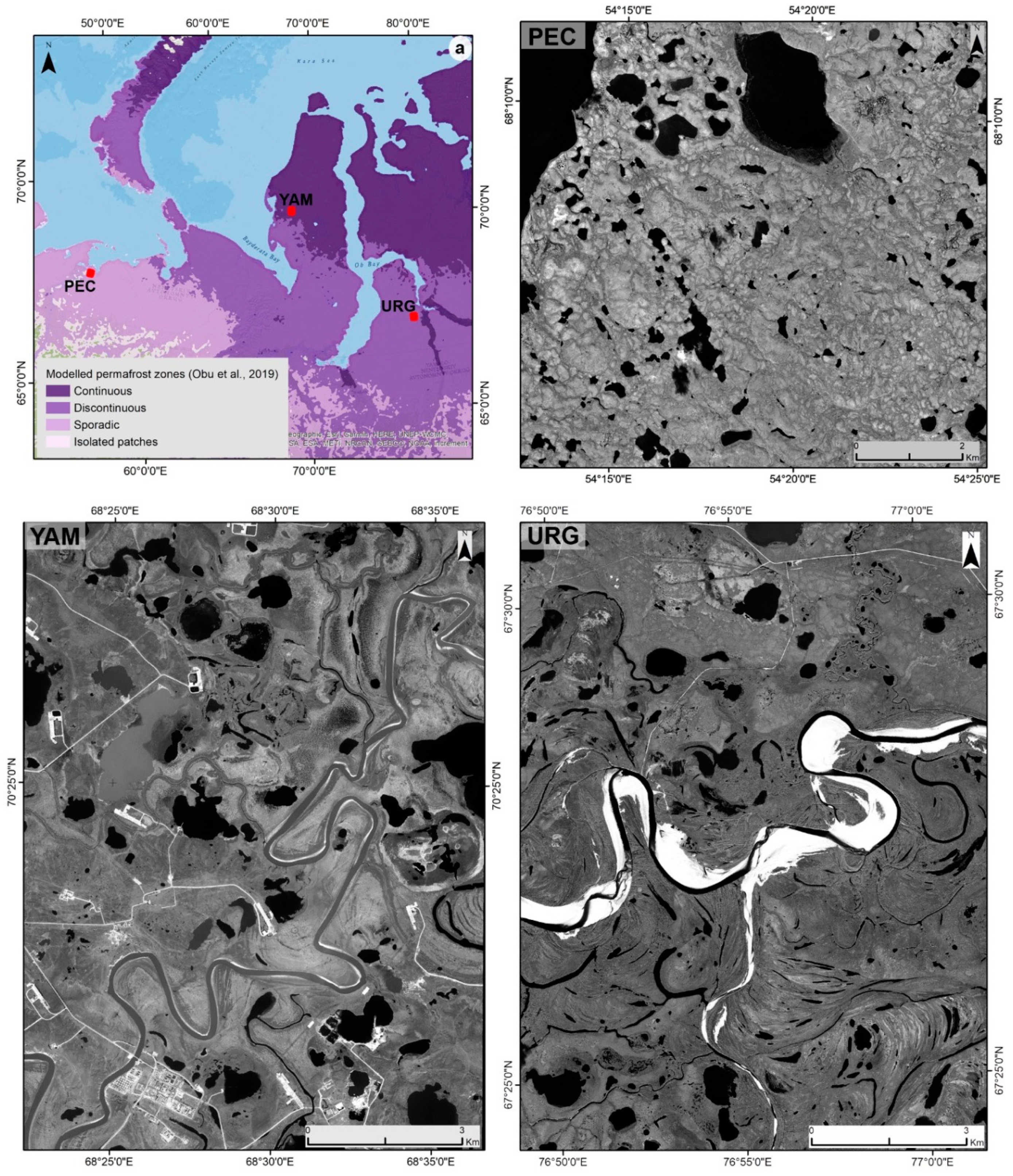
2.1. Study Area

This analysis focuses on three study sites; two are located in West Siberia (Yamal Peninsula—and Urengoy region) (YAM and URG) and one in north European Russia (Pechora delta) (PEC) (Figure 1). The sites are located in continuous, discontinuous and sporadic permafrost regions and cover around 100 km2 each and were chosen as a function of VHR image availability in different years with the largest time span (i.e., 12–14 years). Furthermore, these areas were selected due to the presence of several Circumpolar Active Layer Monitoring (CALM) sites located near these study areas (i.e., Vaskiny Dachi, Urengoy Gas Field GP15 and Bolvansky Cape).
The YAM site is located in the western part of the Yamal Peninsula (70°40′N, 68°48′E), 40 km from the coast of the Kara Sea, on the Bovanenkovo gas field and it covers an area of 122.67 km2. YAM lies within the continuous permafrost zone and based on ERA-Interim data has a mean annual air temperature (MAAT) of −8.3 °C and mean annual precipitation (MAP) of 444 mm (1979–2018). This area has a maximum elevation of 94 m and is dominated by alluvial-lacustrine-marine plains and terraces dissected by rivers (Seyyakha river crosses the area from NE to SW). Several hillslope processes, such as gully erosion [37] and landslides [38], characterize this region. The landscape is dominated by shrub tundra, thermokarst lakes and ponds, as well as poorly vegetated areas affected by landslides (RTS) mostly near the Seyyakha river or lake shores. In this continuous permafrost zone, the permafrost thickness reaches at least 500 m on the marine and coastal-marine plains and reduces to 100–150 m at the younger river terraces [39].
The URG site is located in the Urengoy region (67°45′N, 76°90′E), about 150 km north of Novy Urengoy city in the discontinuous permafrost zone within a tributary of the Pur River basin. This site has a size of 105.09 km2, with a maximum altitude of 30–35 m developed on a marine terrace (Drozdov et al. 2015). URG has a MAAT of −7.4 °C and a MAP of 510 mm. At this site, the permafrost thickness generally reaches 100–300 m [40]. The landscape is dominated by low shrub tundra and contains extensive peatlands [41] and high lake densities [42]. Isolated larch trees also occur, especially near the Pur River tributary crossing the URG site from west to east.
The PEC site is located on the eastern side of the Pechora delta (68°12′N, 54°30′E), at the south of Bolvansky Cape station. It covers an area of 78.43 km2 and lies in the vicinity of the Pechora river in a sporadic permafrost zone. The topography is very flat with elevation up to 40 m and low shrub tundra is the dominant land cover. MAAT at this site is −3.1 °C, whereas MAP is 550 mm. This rolling coastal plain belongs to the southern tundra subzone. The surface lithology consists of Quaternary loams and sands with inclusions of pebbles [43].

2.2. Data Sources

VHR multi-sensor remotely sensed imagery from different years courtesy of DigitalGlobe (http://www.digitalglobe.com), along with high-resolution Corona images, were used to assess landscape changes in the study sites. The selected images have cloud cover of less than 5% and were acquired during the peak vegetation growing season from July to August [44]. All the images used in this study are listed in Table 1.
Along with satellite images from 2003/2004 and 2016/2017, in two of the three analyzed sites, Corona images were used for the assessment of river dynamics. The Corona images are declassified, Cold War era satellite surveillance system images taken from 1963 to 1980, these being panchromatic photographs with large swath widths and varying ground resolutions (0.6–15 m). These images were geo-referenced and co-registered with the newest Quickbird imagery for each site to allow for change detection.
Moreover, for the analysis of retrogressive thaw slumps from the YAM site, a very high-resolution digital elevation model (ArcticDEM) at 2 m spatial resolution (https://www.pgc.umn.edu/data/arcticdem/) and derived parameters were used for the delineation of these features.

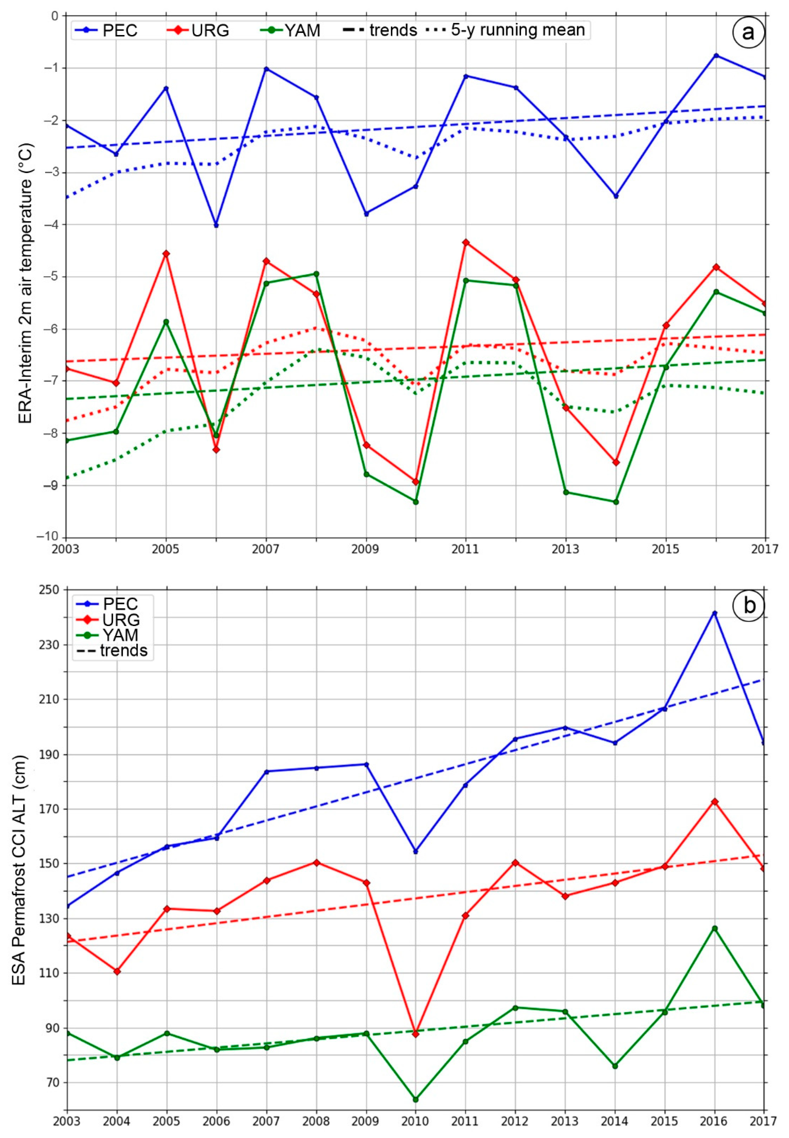
2.3. Climate Data and Active Layer Thickness

As in the study of Chețan et al. [45], climate conditions at geolocations of the three case study areas are inferred from ERA-Interim atmospheric reanalysis [36]. Previous studies [45,46] showed good agreement between climate data from meteorological stations operated by the Russian hydrometeorological observation network (Russian Institute of Hydrometeorological Information—World Data Center, RIHMI-WDC, available at http://meteo.ru/) and ERA-Interim data in our region of interest. This also confirms the results of Lindsay et al. (2014) [47] indicating that ERA-Interim is well suited for high northern latitude applications. Therefore, for this study, we use ERA-Interim data rather than nearby hydrometeorological station data.
Atmospheric reanalysis is a technique of assimilation of meteorological observation data using numerical circulation models. Atmospheric reanalysis intends to remove eventual physical inconsistencies due to deficiency of meteorological observations (e.g., sparse distribution of meteorological stations or shortcomings of observational techniques) and it is considered the most accurate reconstruction of past climate conditions. The horizontal resolution of ERA-Interim is ~75 km.
Following results from Georgievski et al. [46], we have complemented our analysis with the active layer thickness from ESA Permafrost climate change initiative (CCI). The map of ESA CCI active layer thickness [35] is based on the transient permafrost model CryoGrid CCI driven by land surface temperature (MODIS LST/ ESA LST CCI) and land cover (ESA LC CCI). ESA Permafrost CCI maps are available for period 2003–2017, and the spatial resolution is ~1 km. Considering the small-scale heterogeneity medium resolution, ESA Permafrost CCI active layer thickness has been verified against in situ observations documented in the CALM database. The CALM network is a coordinated attempt to standardize measurements of active layer properties in circumpolar regions. Comparison of ESA Permafrost CCI active layer thickness with corresponding CALM sites measurements shows that datasets are either in good agreement (Vaskiny Dachi) or qualitatively good at capturing trends (Urengoy Gas Field GP15 and Bolvansky Cape).
Since CALM data are not available for all the areas covered by VHR imagery, in further analysis we use ESA Permafrost CCI active layer thickness spatially averaged for YAM, URG and PEC regions.
We note that the resolution of the ERA-Interim data is rather coarse compared to the scale of VHR images and may not fully represent the exact conditions at the three sites. However, on the one hand, they can be used to identify large-scale climate drivers of environmental change that also act at small scale and, hence, may contribute to permafrost degradation. On the other hand, it has been shown that ERA-Interim data generally agree well with observations in the high northern latitudes [45,47,48].

2.4. Land Use Land Cover (LULC) Changes

For the analysis of land cover change, a supervised classification of each satellite image was conducted through an object-based image analysis (OBIA) approach. OBIA is now a widely accepted and used alternative, demonstrated as superior to pixel-based methods [49,50,51]. For comparison purposes, each site was classified into 6 classes: water, shrub tundra, grassland and sparse vegetation, disturbed inundated areas and barren including artificial surfaces.
The first step of the supervised classification consists of delineating training and validation samples. The polygons (samples) have been delineated for the analyzed years, within each study area. Each polygon was manually delineated on the true color satellite image, aided by the panchromatic band, covering a unique land cover class. The areas were chosen such that the land-cover class could be clearly identified on the image. To independently assess the accuracy of land cover maps, the total number of samples was randomly split into training samples (70%) and validation samples (30%), before the classification procedure.
The OBIA land cover classification was conducted using eCognition Developer software, version 8.9, starting with the image segmentation process and resulting in automated delineated polygons (objects) by merging contiguous pixels from the four spectral bands. Subsequently, the resulting objects have been classified into land cover classes using the Random Forest (RF) machine learning method [52]. The RF method has proved to be among the most accurate and widely used methods for land cover classification, since it is robust, has capabilities to work with various data types and it is not affected by statistical data distribution [53,54]. Mean and standard deviation of the pixel values within training objects, for each of the four spectral bands, were used as input features for the RF classification process with 500 decision trees. The RF classification resulted in a land cover map for each year and study area, with the five pre-defined classes.
The accuracy of each land cover map was independently assessed based on the validation sample dataset, regarding the widely used metrics of overall accuracy (OA), Cohen’s kappa index of agreement (KIA), producer’s accuracy (PA) as omission error and user’s accuracy (UA) as commission error [55].

2.5. Water Bodies and Fluvial Dynamics

Based on the results from the landcover classification using object-based image analysis and random forest, connected pixels of class water were aggregated into objects. From all resulting water bodies, the rivers were manually excluded, and the remaining objects were exported as polygons and classified as lakes and ponds based on a threshold areas of 100 m2 [25]. The generated polygons were then used to assess changes in lake area and lake abundance in each case study region during the observation period. Moreover, the lakes/ponds were classified based on the magnitude of changes into disappeared, new, relatively stable (up to 5% areal extent changes), shrinking and growing for each site.
The planform changes of two different river channels in YAM and URG were analyzed. We used four scenes (1961, 1976, 2004 and 2016) to detect subtle changes in the Seyyakha river channel and three (1967, 2003 and 2017) for the tributary of Pur. Digital methods that parse the data derived from remote sources (e.g., satellite images, orthophotos) are very suitable for detecting the changes that occur in river channels. To quantify the rate of spatio-temporal changes in watercourses, vector polygons were generated for each analyzed year.
For each polygon, the centerline that follows the configuration of the minor riverbed was extracted using the Polygon to centerline toolbox in ArcGIS 10.4.1. This helps to evaluate the total length of the river and, at the same time, is the base file for the channel investigations.
To assess channel shifts and the rates of lateral migration, we used the Channel Migration Toolbox [56]. Using the Transect tool that automatically generates perpendicular lines on the centerline of the river course, channel width at every 100 m was calculated. The mean values of flow direction correspond to the azimuth of transect lines generated by Digital Shoreline Analysis System (DSAS) version 5.0 [57]. Likewise, to establish the channel type, the sinuosity index was calculated using the Sinuosity tool by dividing the length of the centerline by the straight line distance between the end points of the channel.
Based on each channel polygon, the fingerprint of the main geomorphic processes was calculated. The total amount of land surface erosion and deposition was determined as the difference between the pairs of channels for the available imagery (1961–1976, 1976–2004, 2004–2016, for the Seyyakha river sector from Yamal; and 1967–2003 and 2003–2017, for the tributary of the Pur River).

2.6. Landslides and Infrastructure

We examined the occurrence of RTS in the YAM site on the multispectral images from 2004, 2016 and available digital elevation model (DEM) and manually digitized all the features. Both polygon datasets were counted and their corresponding area calculated. The headwall of each landslide was manually digitized in both scenes and then the longitudinal change in each case was measured in ArcGIS. Longitudinal transects were drawn at every 1 m between the 2004 and 2016 headwalls and the mean annual value of retreat was calculated for each feature.
The infrastructure components were also manually digitized on two different datasets (2004 and 2016) in the Yamal Peninsula using ArcGIS 10.4.1. Roads and buildings were digitized as polygons and pipelines as lines in both datasets.

3. Results

3.1. Climate Drivers of Environmental Change

Annual mean 2 m air temperature increased in the period from 2003 to 2017 at the geolocations of all three sites (Figure 2a). The linear trend analysis using the least-squares method shows the most substantial increase at PEC (~0.6 °C/decade), a slightly weaker increase at YAM (~0.5 °C/decade) and the lowest increase is detected at URG (~0.3 °C/decade). Georgievski et al. (in preparation) analyzed climate patterns relevant for permafrost degradation and identified abrupt warming events (years with annual mean temperature warmer than the 5-year running mean temperature) have a high impact on deepening of active layer thickness. The comparison of Figure 2a,b shows that this is also a valid assumption for the three sites; as the warm year events coincide with the strongest deepening of the active layer. Furthermore, the corresponding linear trends show the strongest deepening at the PEC site (~51.5 cm/decade), while at the URG and YAM sites, active layer thicknesses increased by ~22.7 cm/decade and ~15.3 cm/decade, respectively.
Although the YAM site is warming at a faster rate than URG (~0.5 °C/decade vs. ~0.3 °C/decade) during the considered period, the latter site is characterized by a quicker deepening of the active layer (~22.7 cm/decade vs. ~15.3 cm/decade). This probably reflects the impact of changes in the hydrological cycle. Though the annual mean precipitation shows a notable declining trend during the VHR observation period (2003–2017) at all sites (YAM: −3.2 cm/decade, URG: −1.3 cm/decade, PEC: −6.9 cm/decade), there is no significant change in the precipitation trend during the whole ERA-Interim period (1979–2018) except for a slight increase at the PEC site. However, seasonal variations in precipitation, in particular, the increasing trend during the transition months between winter and summer (March, April and May), may lead to changes in snow cover that can have a critical impact on the active layer thickness. A trend analysis of the snow water equivalent (SWE) shows almost the same increase in the annual mean for both the YAM and URG sites (~3 cm/decade), where at the latter site it shows a much stronger increasing linear trend in the month with maximum SWE (~11 cm/decade vs. ~5 cm/decade). Therefore, it is very likely that the active layer at the URG site does not completely freeze during the months with maximum SWE as the deeper snow cover leads to better isolation of the soil from the cold surface than at the YAM site. In a warming climate, this can compensate for a slower warming of the air temperature and, hence, result in a stronger trend in the deepening of the active layer. The PEC site shows a fragile increasing trend for both annual SWE (~0.8 cm/decade) and maximum SWE (1.5 cm/decade). Therefore, the primary driver of active layer deepening at the PEC site during the considered period (2003–2017) is the increase of mean annual air temperature, while at the YAM and URG sites changes in hydrologic cycle seem to modify the impact of warming on the deepening of active layer thickness. Trends of increasing SWE at our sites support findings of Bulygina et al. [48] for the previous period based on snow depth observations. They also found increasing trends of maximum snow depth in the Western Russian Arctic.

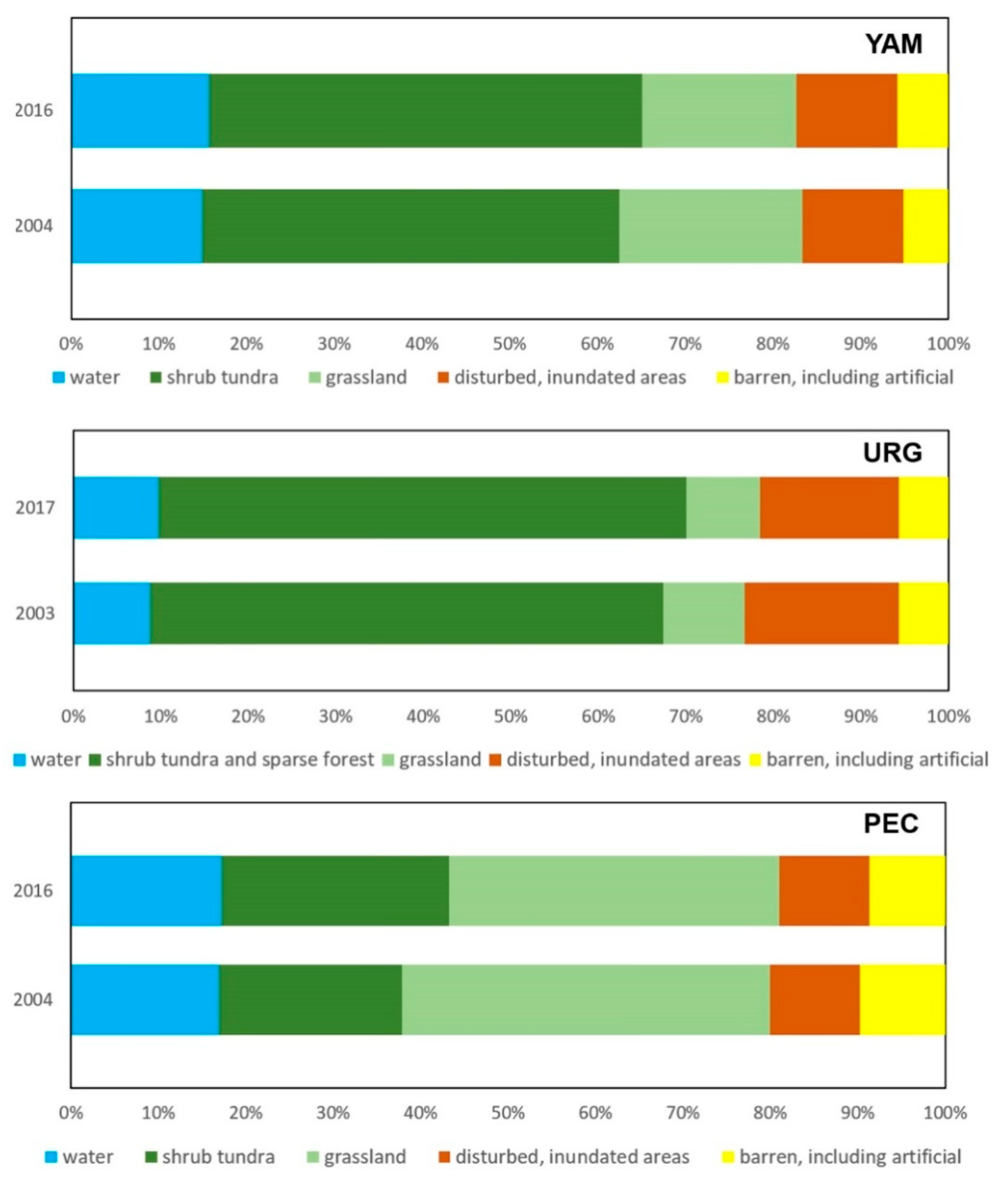
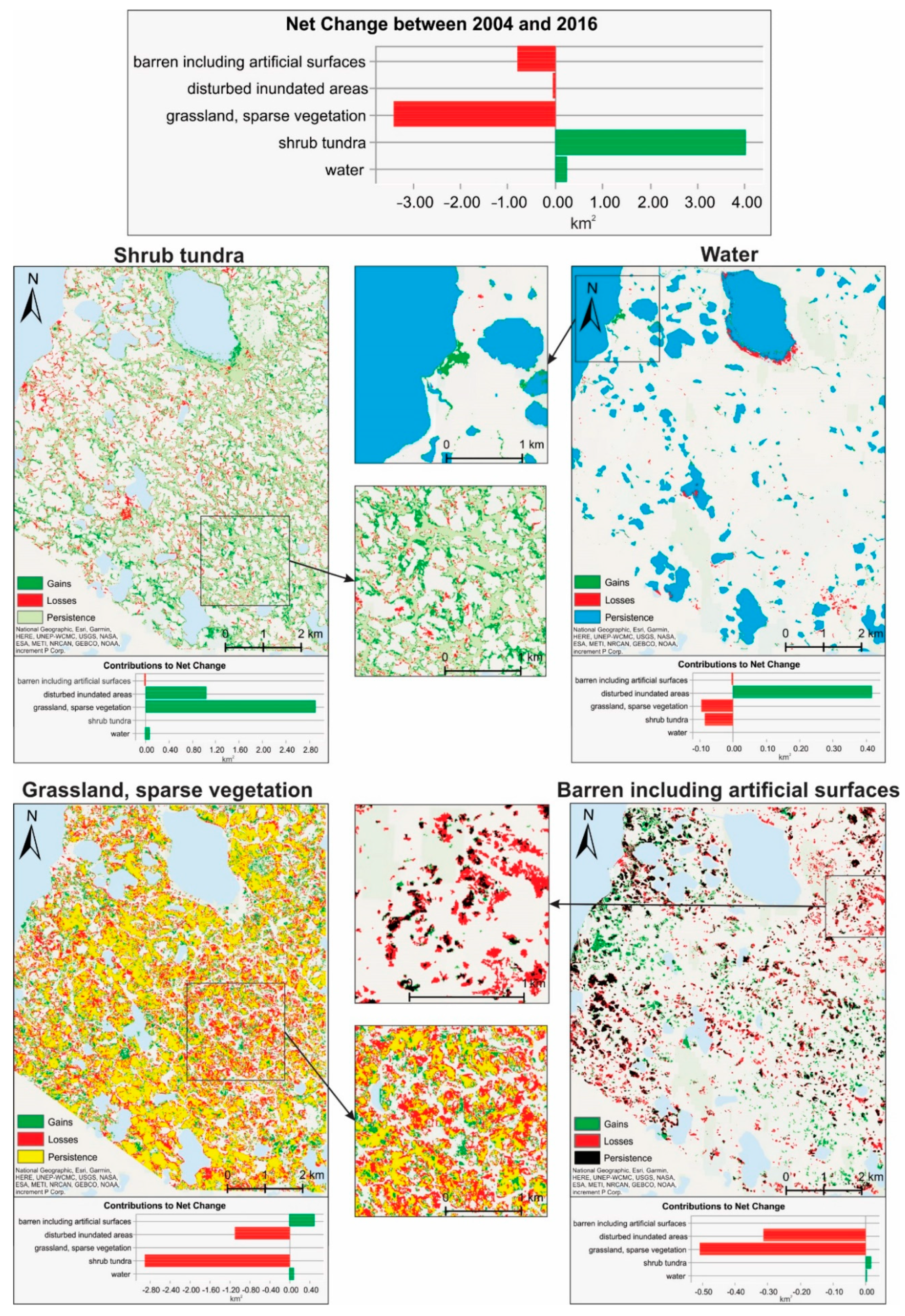
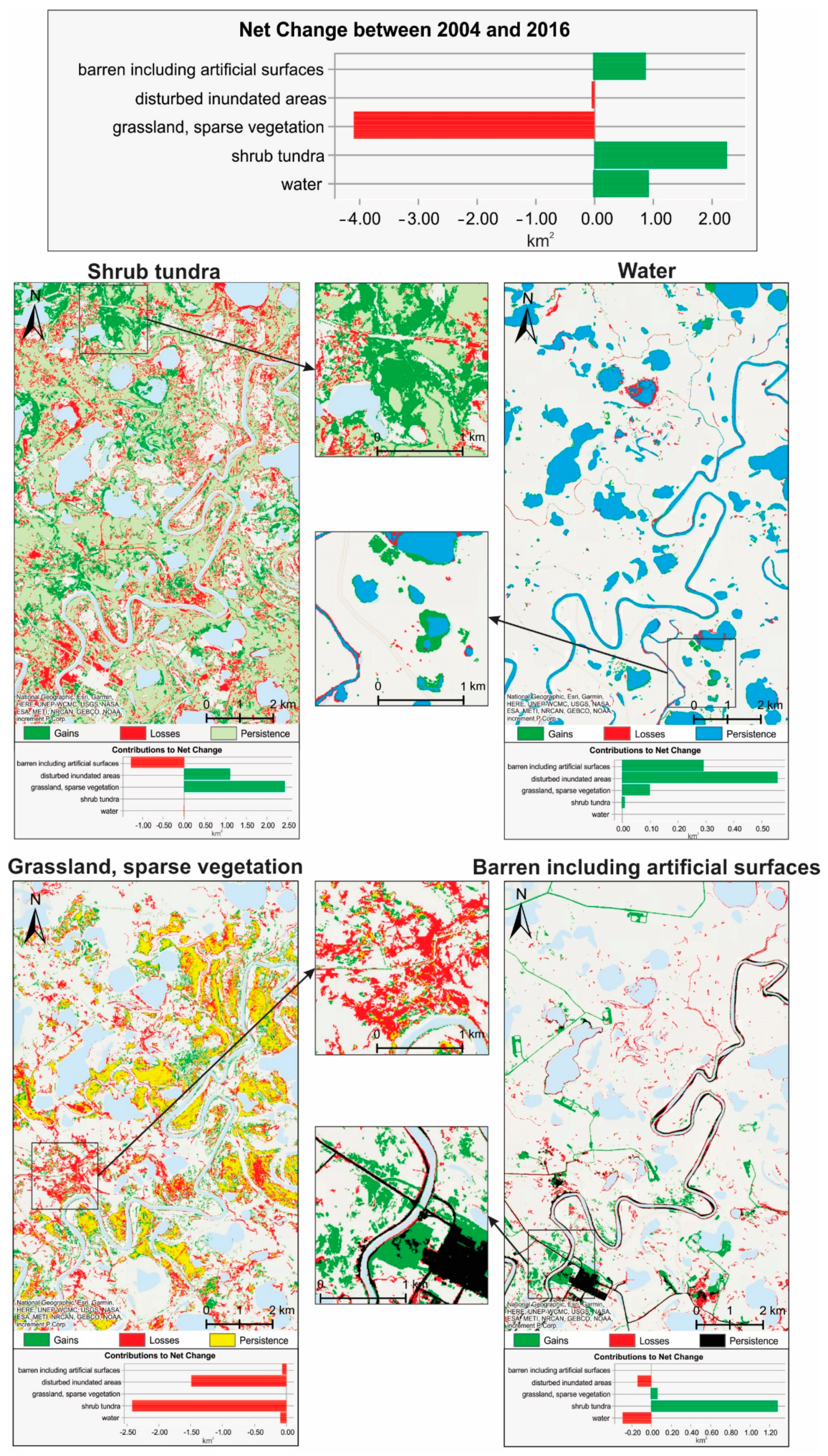
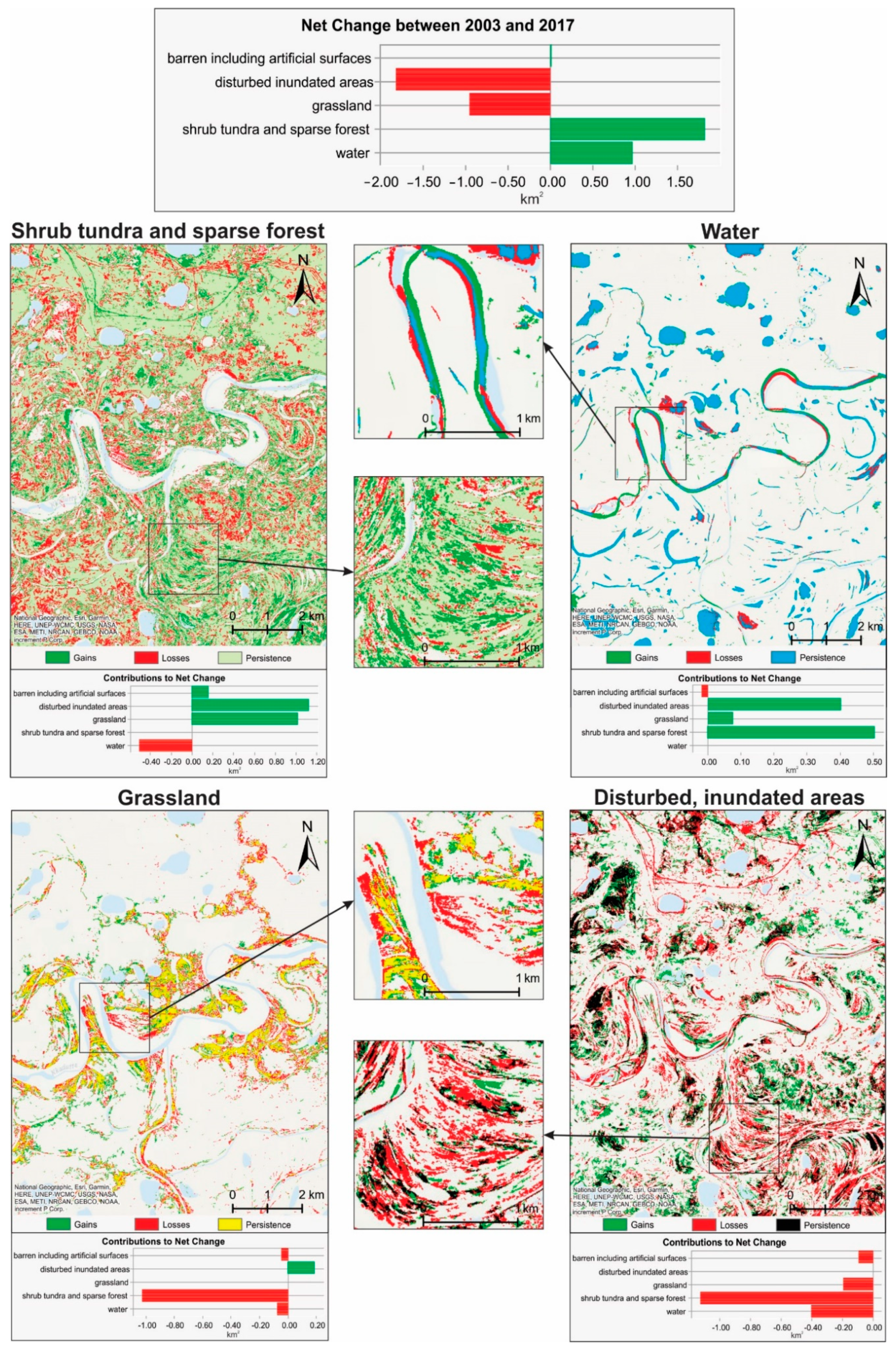
3.2. Land Use Land Cover (LULC) Changes

The comparison of major land cover fractions between the VHR scenes shows a general decrease of grassland and an increase of shrubs and water classes in all sites (Figure 3). Here, the increase in water classes is most evident at the discontinuous permafrost URG site.
Overall, the generated land cover maps recorded excellent accuracy values with OA ranging from 0.91 to 0.95, while KIA ranges between 0.87 and 0.93 (Table 2). As expected, the high accuracy values (close to 1) were achieved for the water class due to their notable spectral separability. Shrub tundra, including sparse forest in the Urengoy site, also yielded very high accuracies ranging from 0.85 to 0.99, with eleven cases out of twelve that have values higher than 0.91. Barren, including artificial surfaces, recorded accuracy values higher than 0.85, except within the Yamal study area in 2004. The disturbed, inundated areas and grassland classes mostly have excellent accuracy values, although there are a few outliers where UA reaches lower values such as 0.63 in the Pechora study area in 2004 and 0.43 in the Yamal study area in 2004 (Table 2).
For the Pechora site, the shrub tundra class showed the largest dynamics between 2004 and 2016, when it extended its area by 24.4% (4 km2) homogeneously across the study area. Here, the replaced classes mostly comprise grassland/sparse vegetation (72.5%, 2.9 km2) and disturbed, inundated areas (26%, 1.04 km2). On the contrary, grassland/sparse vegetation, and barren, including artificial surfaces, areas decreased by 10.3% (3.4 km2), concentrated in the south-east and western part, and 10.5% (0.8 km2) concentrated in the north-east, respectively. Grassland/sparse vegetation, besides shrub tundra, lost area due to the expansion of disturbed, inundated areas (1.1 km2), while barren class, was replaced by grassland of 0.51 km2 and disturbed, inundated areas of 0.31 km2. Water surface area increased in the analyzed interval by 1.7% (0.23 km2), with expansions mainly localized around small lakes and the northwestern shore. The disturbed, inundated areas class showed the lowest net change with only −0.04 km2 (Figure 4).
The same tendencies have been observed for the Yamal study area, except barren and artificial surfaces, which recorded a positive net change of 14.5% (0.91 km2). They mainly replaced shrub tundra (on 1.28 km2) and grassland (0.07 km2). Here, new roads were identified on the map in the northern and western part of the study area, accompanied by new buildings occurring during the analyzed interval. A net gain of 3.86% (2.25 km2) was observed for shrub tundra, mostly replacing grasslands (2.42 km2) and disturbed, inundated areas (1.12 km2), predominantly in the northern and western part of the study area. However, part of this gain was compensated for by a loss of 1.28 km2 to artificial surfaces. The surface water area increased by 5.17% (0.95 km2) through lake expansion replacing disturbed, inundated areas (0.56 km2), barren, including artificial surfaces (0.29 km2) and grasslands (0.1 km2). Grasslands lost 15.88% (4.08 km2) due to shrub development of 2.42 km2 and the expansion of disturbed, inundated areas of 1.49 km2, localized mainly in the south-western part of the study area (Figure 5). Similar to Pechora, the disturbed, inundated areas showed the lowest net change (−0.04 km2).
For Urengoy, positive net changes have been observed for shrub tundra and sparse forest (2.94%) and water bodies (10.53%), negative net changes for grassland (9.83%) and disturbed, inundated areas (9.83%). In contrast, the barren area (including artificial surfaces) did not change during the analyzed interval. Shrub tundra and sparse forest developed mainly at the expense of disturbed, inundated areas (1.13 km2), grassland (1.03 km2) and barren land (0.17 km2), with new patches predominantly appearing in the south-eastern part. Water bodies mainly replaced disturbed, inundated areas (0.4 km2), shrub tundra and sparse forest (0.51 km2) and grassland (0.08 km2), mainly due to changes in the river watercourse and appearance of new lakes. Grasslands and disturbed, inundated areas primarily developed into shrubs, with the latter also changing to pristine lakes (Figure 6).

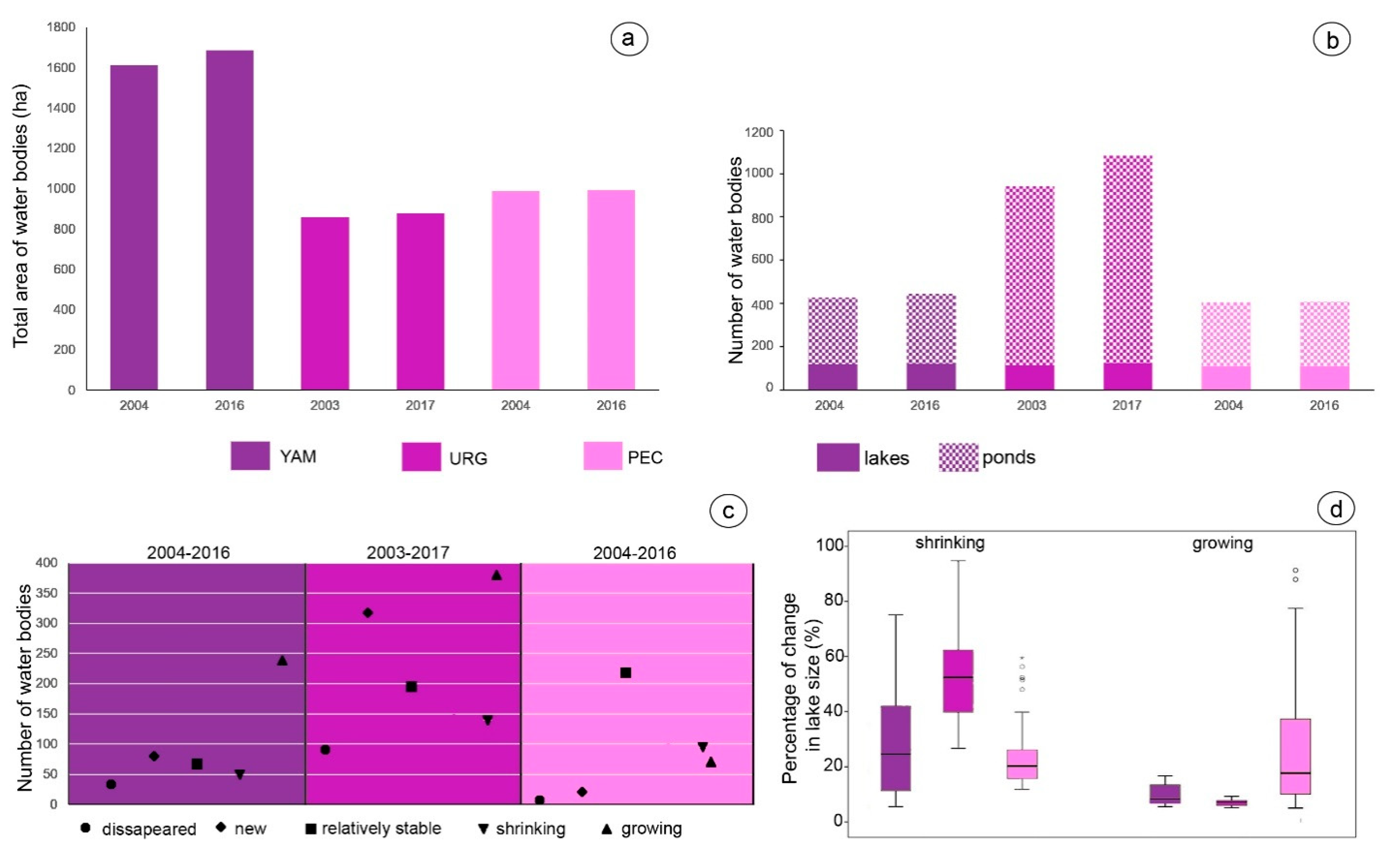
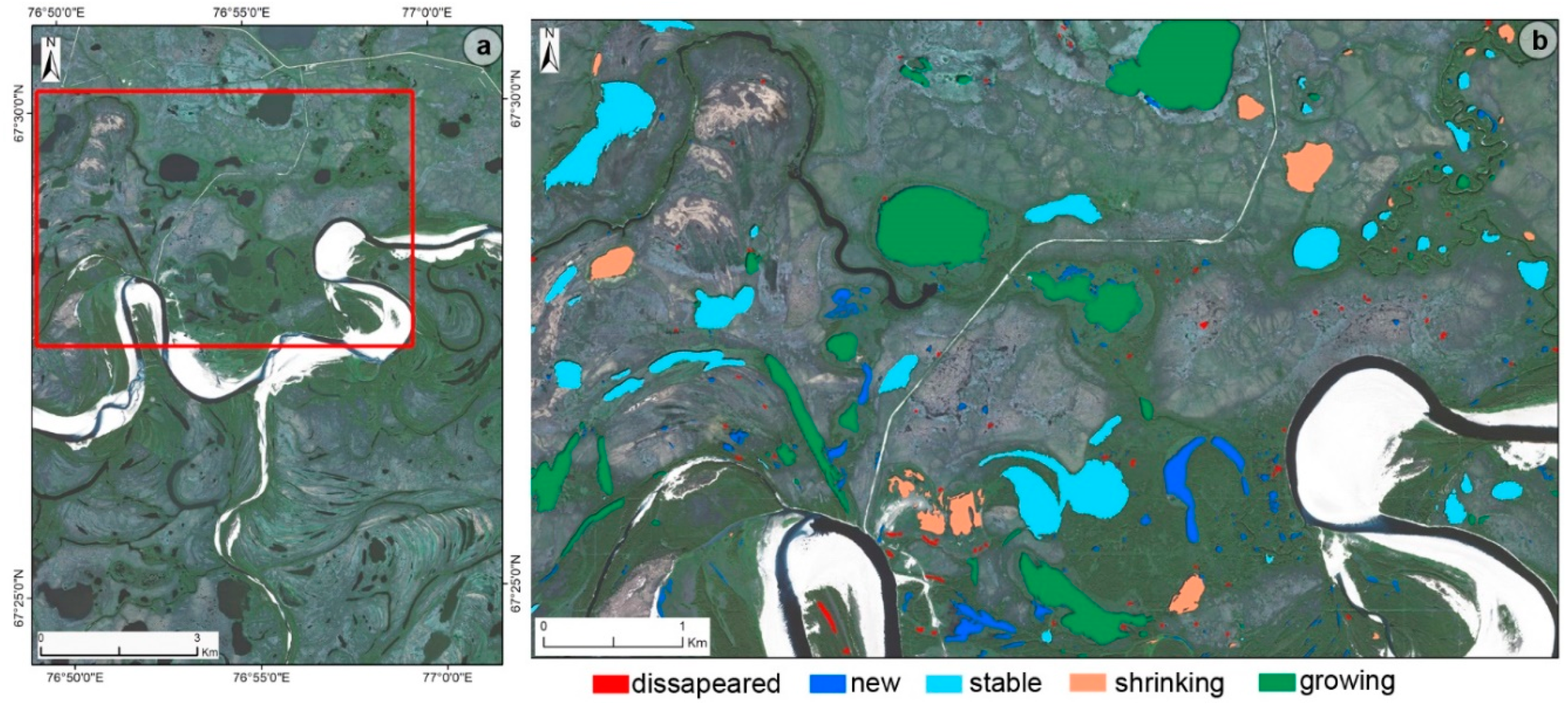
3.3. Water Bodies (Lake/Ponds) Dynamics

The total area covered by lakes and ponds larger than 0.01 ha slightly increased in each case study region. The total water bodies surface area increased by 0.45% and 4.72% in PEC and YAM, respectively, whereas in URG, the area covered by water bodies larger than 100 m2 expanded by 2.38% during the observation period (Figure 7a). Half of the lakes and ponds remained predominantly stable in PEC, whereas in URG and YAM the majority of the water bodies show an increasing trend. In URG, 317 new lakes and ponds were initiated between 2003 and 2017, whereas in PEC, only 20 newly-formed water bodies appeared during the 12-years interval (Figure 7c).
The number of lakes and ponds larger than 0.01 ha increased by 0.74% in PEC, 4.46% in YAM and 14.86% in the URG region during the observation period. Ponds are the dominant type of water bodies in each study site (e.g., YAM—73%, URG—88.5% and PEC—73.2%). Both lakes and ponds increased in number in URG and YAM, whereas in PEC, only ponds experienced an increase, whereas lakes number remained stable (Figure 7b).
The mean lake area changed slightly in PEC (−0.28%) and YAM (+0.1%), and decreased considerably in URG (−10.75%). Despite the lake density in URG (10.2/km2) is twice as large as in PEC (5.2/km2) and YAM (3.6/km2), the average size of inventoried lakes is smaller in URG (8 ha vs. 40 and 20 ha, respectively). The increase in the number of ponds in URG is a result of thermokarst processes but is also related to the partial drainage of larger lakes.
Although the majority of water bodies are growing, the fraction of change per individual lake (%) is more significant for shrinking lakes (Figure 7d). By far, the most remarkable changes over the analyzed interval occurred in discontinuous permafrost area (Figure 8).

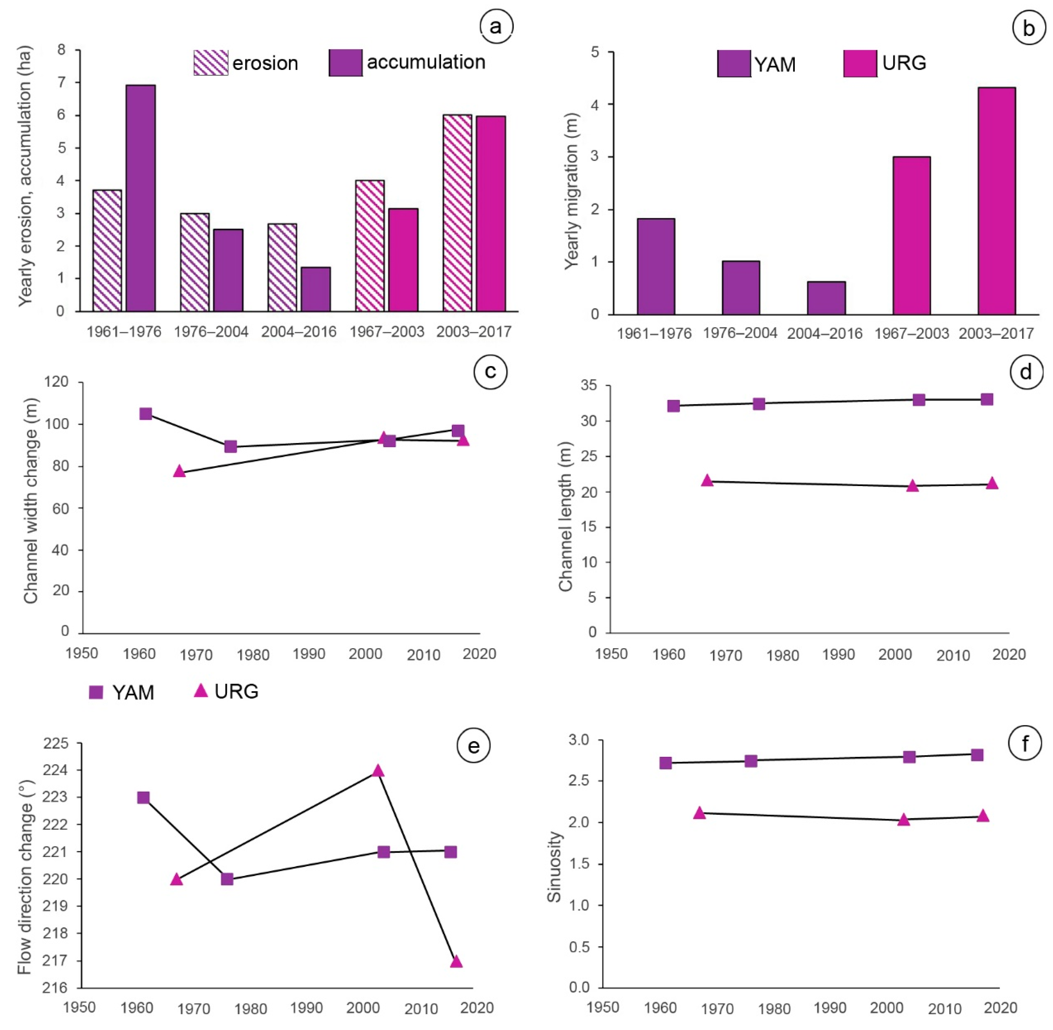
3.4. Fluvial Dynamics

For at least six months per year, snow and ice cover the drainage networks in these regions, thereby decreasing the intensity of in-channel geomorphological processes [58]. The erosion is dominant in both analyzed cases, except from 1961 to 1976 for the Seyyakha river (YAM) (Figure 9a). The annual erosion rates have greater values for the tributary of the Pur river (URG). Still, between 2004 and 2016 the erosion was barely twice as high as the accumulation ratio for the Seyyakha river.
The length of the Seyyakha river increased by 0.65% in the first period, 1.71% in the second period and 0.42% in the third. The length of the river in URG decreased in the first phase (3.4%) but increased (1.79%) between 2003 and 2017 after new meander bends were initiated (Figure 9d). The sinuosity index of the Seyyakha river increased in all periods as the meanders continuously developed (Figure 9f). In URG, the initial decrease of the sinuosity was followed by a slight increase in the last years.
Channel migration is a natural phenomenon as rivers try to reach a dynamic equilibrium state. The migration rates for the Seyyakha river indicate a mature stage and a quasi-stable channel, with annual migration values between 1.8 m (1961–1976) and 0.6 m (2004–2016). The Pur tributary is more dynamic, with mean annual values of migration rates around 4 m (Figure 9b). Regarding the changing rates for the flow direction, there are no significant shifts (Figure 9e). The differences in azimuth for the Pur tributary in URG (0.22°/year) are larger than the corresponding values for the Seyyakha river in Yamal (0.07°/year). Furthermore, the results for the channel width values indicate a cumulative change of ~17 m for the Pur tributary and ~24 m for the Seyyakha river (Figure 9c).

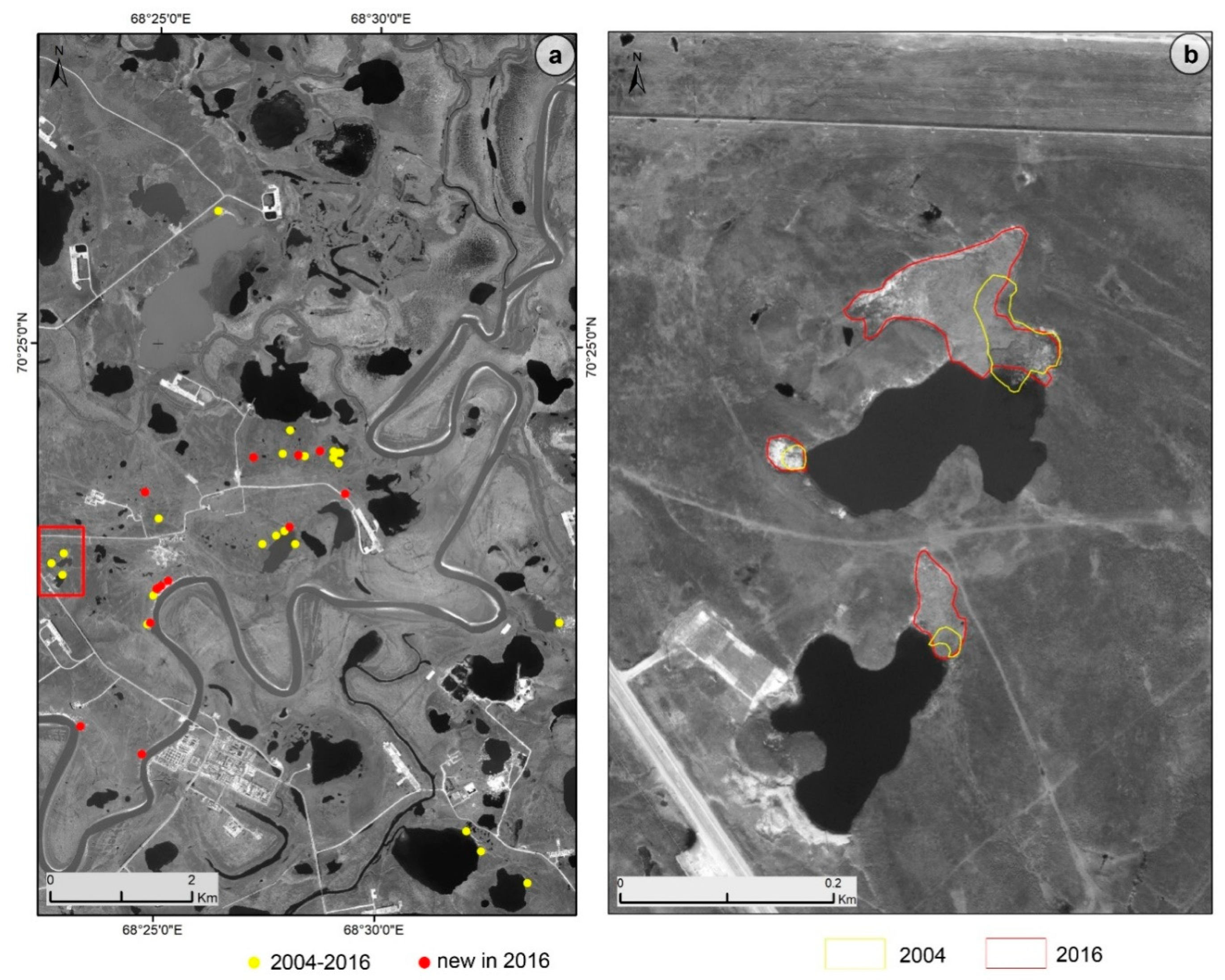
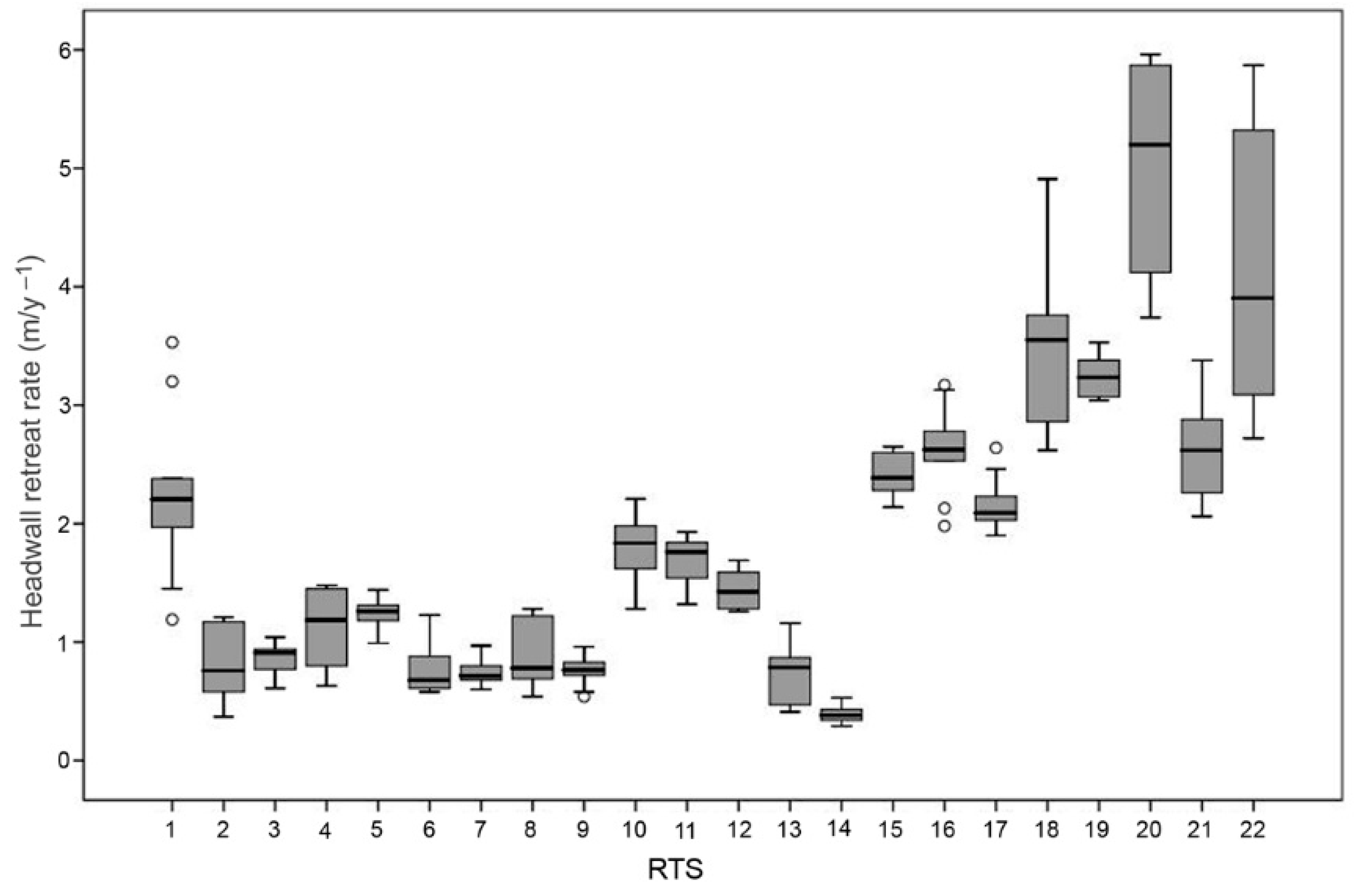
3.5. Retrogressive Thaw Slumps
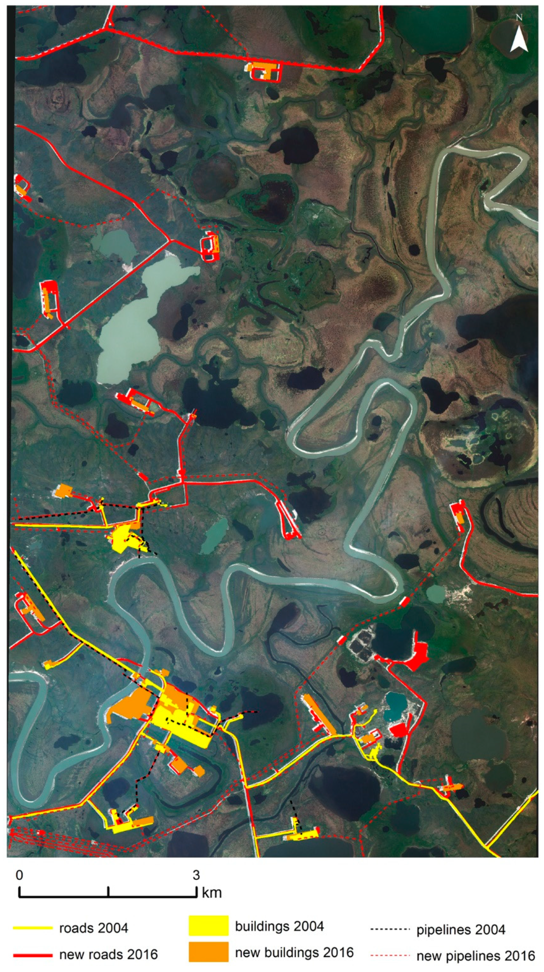
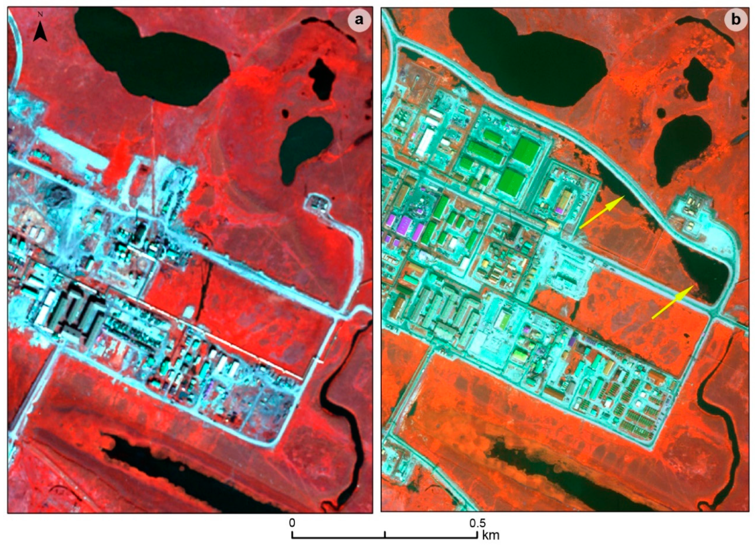
In the Yamal Peninsula, the majority of retrogressive thaw slumps (RTS) were identified in sloped terrain along lakeshores and the Seyyakha River (Figure 10).
RTS generally occur in clusters where favorable site-specific conditions for their development exist. For Yamal, RTS are abundant in the western part and were initiated by thermo-erosion and mechanical erosion due to fluvial processes and waves. In a few cases, the development of RTS is related to the melting of ice-wedge polygons, known as “baydjarakhs” [59]. The features cover small spatial footprints ranging from 0.01 to 1.32 ha (mean area: 0.26 ha). The majority of the features have lengths/widths lower than 100 m and in some cases present evidence of coalescence. Furthermore, 51% of the RTS have a length to width ratio below 1. The number of RTS increased from 24 in 2004 to 37 in 2016 whereas the total area of thaw slumps had grown by about 69% for the same interval. The mean rate of slump headwall retreat ranged between 0.3 m/year and 4.9 m/year uring the period from 2004 to 2016. Based on the VHR satellite images from 2004 and 2016, the mean rate of RTS growth was between 11 and 679.8 m2/y (Figure 11).

3.6. Infrastructure

In the Yamal Peninsula, enormous unexploited gas resources were discovered in the 1980s. Since then, an extensive network of roads, drilling sites, buildings and gas pipelines appeared around the significant gas deposits. In the investigated site within the Bovanenkovo gas field, the total area covered by infrastructure constructions (roads and buildings) increased from 107.08 to 308.02 ha between 2004 and 2016 (Figure 12). The surface covered by roads expanded by 3.7 times, whereas the total area of buildings increased by 2.2 times during the 12-years interval. Moreover, the entire length of gas pipelines increased by 7.4 times in the same period. The expansion of the infrastructure in YAM was related to notable changes in hydrological features (Figure 13). In YAM, no footprint of roads, buildings or pipelines is found in the 1961 and 1976 Corona images. In PEC and URG, the buildings are sparse and concrete roads are entirely missing.

4. Discussion

VHR sensors (e.g., QuickBird, WorldView, GeoEye) have the potential to reveal subtle landscape changes in the permafrost dominated landscape and to overcome the limitations of medium and low-resolution satellite images [60]. Although the latter satellite images are preferred for extensive mapping of broad-scale vegetation or water bodies, these datasets are inappropriate to capture local high spatial heterogeneity of land use classes in Arctic regions [61]. The use of multispectral VHR data proved to be ideal for detecting different categories of land cover and for assessing a wide variety of disturbances. These images are also essential to enhance the fuzzy boundaries delineation of various types of land cover (e.g., water, sparse vegetation, shrubs).

4.1. Regional Climate Impact on Permafrost Degradation

Identifying climate changes on the regional scale that drive the local environmental change in the high northern latitudes remains a challenge [62]. Here we explore the role of regional climate drivers obtained from ERA-Interim (~75 km horizontal resolution) on the processes that are hypothesized to affect processes of the ecosystem and environmental change on the local scale. The active layer deepening indicated by data from ESA Permafrost CCI (~1 km horizontal resolution) serves as a link between the low-resolution climate data and the VHR remote sensing data. In the considered period at the three study sites, we find that warming is the primary driver of deepening of the active layer, while changes in the hydrological cycle can modify the impact of warming. Warm air and ground temperatures, changes in precipitation and deep snow have been recognized as major climatic drivers affecting permafrost degradation [63], for example, expressed by deepening of the active layer, RTS and thermokarst lake formation. At our three study sites, warming and increased SWE have been identified to act in favor of deepening of the active layer, which consequently results in an increasing number of RTS and thermokarst lake formation. Changes in vegetation can further amplify the impact of increasing SWE. For all three regions, an increase in shrub tundra is documented. This type of vegetation is prone to trap snow, which keeps the ground insulated so that warmer soil temperature can be maintained during the cold season.

4.2. LULC Changes and River Dynamics

Our analysis revealed accelerated land surface dynamics across three different permafrost zones in western Siberia and northeastern European Russia. A pronounced increase in the extent of tundra shrubs was found in all cases. This is in agreement with previous findings, which considered this type of Arctic disturbance as a critical driver of tundra greening [64,65,66,67,68,69]. In the three investigated Arctic study sites, recent expansions in shrublands were associated with the loss of the grassland and sparse vegetation class. Based on experimental and observational research, previous studies revealed that climate warming is the driving factor of the so-called Arctic “shrubification” [70]. Compelling pieces of evidence for the latitudinal shrub lines advancing in response to warming atmosphere temperatures were presented in different studies [71,72,73,74]. Furthermore, the increase in productivity of Arctic tundra is frequently related to recent summer warming [45,75,76].
The transition from land to water is another spatially extensive change taking place in each of the three study sites. Water area gain is subject to thermokarst activity, which is responsible for new pond formation, lake basin expansions and river widening in YAM and URG. In discontinuous permafrost (URG) the growth of water surfaces was twice as large as in continuous permafrost (YAM), whereas, in sporadic permafrost (PEC), we noticed only a slight increase. In all three study sites, ponds (below 1 ha) are the dominant water body type, as elsewhere in the Arctic lowlands [21,25].
Unfortunately, the dynamics of Arctic ponds have received comparatively little attention due to the limited availability of VHR images. The existing global inventories of lakes derived from Landsat data [77] have large inaccuracies in permafrost environments [20]. By using VHR images (spatial resolution < 5 m), ponds as small as 0.01 ha can be accurately delineated [25,78]. A direct comparison with the PeRL database [25] revealed good correspondence between our findings and similar analyses using VHR data. Thus, for the YAM site, we mapped 445 water bodies, whereas, in PeRL database, 443 features larger than 0.01 ha were inventoried [25]. The increase in number and surface area of lakes and ponds in the three Arctic sites agrees with other similar analyses in high latitude environments [79,80].
The variation of channel characteristics relates to transport and deposition of load amount, and with specific fluvial and thermal erosion [81]. Our results indicate the dominance of erosion during the last two decades, whereas in-channel accumulation characterized the 1961–1976 period in the Seyyakha River. Both considered rivers revealed a tendency of a slight increase in their lengths between 2003 and 2017. The imbalance between erosion and accumulation also led to changes in width, sinuosity and river flow direction [81]. Because erosion of banks is almost twice as large as the accumulation at Seyyakha, a significant widening of the river was observed in the last decades. Here, the fast retreat of ice-rich river banks is initiated by a combination of mechanical and thermal erosion [82]. An increase of the fluvial thermal erosion due to rising water temperature during the flood season was observed in the last decades [83]. This increase in water temperature might explain the recent widening of Seyyakha.
In the case of Seyyakha, the annual lateral migration of the channel is similar to other results reported in the Mackenzie Delta [81,84]. The river channel mobility in the Urengoy is twice as high, mainly due to the rapid evolution of small meandering channels. However, since the annual rates of fluvial channel changes are subtle in both YAM and URG, the available coarse-resolution products are inappropriate to resolve local scale river-banks variation.

4.3. RTS Landslide

Because thaw slumps in the Arctic regions are commonly small-sized features, they are below the detection limit of medium resolution satellite images (e.g., Landsat) [20]. VHR satellite images allowed identifying thaw slumps as small as 10 m in diameter within the Bovanenkovo field. The morphology and distribution of identified RTSs do not differ from similar features described in Central Yakutia [18], Banks Island [85], Yamal Peninsula [86] or Ellesmere Island [87]. We have identified small features in the vicinity of Seyyakha River with areas generally lower than 1 ha. Only two RTSs reach a maximum size of 13,000 m2. In the Yamal Peninsula, the RTS are preferentially localized along the lake/river shores. The abundance of these features in ice-rich conditions along rivers and lake shores was described in many other regions in the Arctic [18,88,89]. Our analysis revealed an evident increase in the occurrence of RTSs between 2004 and 2016. Similar findings were reported by other recent studies in the Arctic regions [85,87,90,91].
Retrogressive thaw slumps and “baydjarakhs” are generally considered as indicators of permafrost degradation in continuous permafrost zones [18,58,92]. Once the scarp of the RTS is created by ice-rich permafrost thawing, a further thaw is expected as permafrost is more exposed in this way [58]. Thus, the thaw slump expands by retrogressive thermo-erosion with rates usually ranging from centimeters to tens of meters per year [93]. The analysis of 22 RTSs in the Yamal Peninsula during the period from 2004 to 2016 provided a mean headwall retreat rate for all RTSs of 1.86 m/y. In comparison, Ward-Jones et al. [87] reported a mean retreat of 6.2 m/y for Ellesmere Island and Lantuit and Pollard [94] found 9.6 m/y for the coast of Herschel Island (Canada). On the other hand, our headwall retreat rates appear to be higher than the values provided by Lantz and Kokelj [88] for the Mackenzie Delta (0.5 to 1 m/y), but similar to Séjourné et al. [18] for Central Yakutia (0.5 to 3.16 m/y).

4.4. Infrastructure

An expansive industrial infrastructure occurred in the Yamal Peninsula between 2004 and 2016. In YAM, the intense human pressure is associated with hydrological disturbances and vegetation disappearance. The increased human pressure stimulated the initiation of new thermokarst features (Figure 13), such as in other ice-rich permafrost landscapes [95]. The observed land cover disturbances are usually accompanied by the modification of the ground thermal regime [63], causing substantial adverse impacts on fragile and sensitive Arctic ecosystems.
The main disadvantages of VHR satellite imagery are their high price and limited availability. However, previous studies have shown the capabilities of both VHR and medium-resolution satellite images. Thus, the surface area of water extracted from Landsat-5 TM amounted to 44–95% of the total surface area [21], whereas Sentinel-2 show promising results when mapping water bodies larger than 350 m2 (Freitas et al., 2019). However, the delineation of small water bodies’ boundaries is problematic when the pixel footprint does not lie entirely within the water body [96]. Landsat satellite images allowed the identification of only 25% of the total number of landslides in Himalaya [97] while SPOT images prevent the identification of about 30% of the small landslides in Hong Kong [98]. In the Western Russian Arctic the majority of the thaw slumps are too small to be detected by medium resolution satellite imagery, whereas the calculation of headwall retreat rate is feasible only if using VHR satellite or aerial images with sub-metric accuracies. The river’s water surface delineation revealed that Planet imagery (3 m spatial resolution) allows accuracy of only 3% greater than Sentinel-2 data [99]. Because the size of individual features of infrastructure (e.g., roads and buildings) is very small specific spatial resolution imagery is required for their identification. The inventories of build-up areas based on Landsat are incomplete and lack subcategories [100]. In particular cases, Sentinel-2 allows identification of 3 m wide roads [101].

5. Conclusions

Our study demonstrates the usefulness of VHR satellite data for the detection of smaller features and quantifying subtle changes in Arctic environments. These data allow assessing a wider variety of changes in the permafrost environments compared with medium and low-resolution satellite images. In addition, we linked the scale of regional climate drivers inferred from global ERA-Interim reanalysis via the intermediate resolution ESA Permafrost CCI product to the scales at which the processes hypothesized to affect local vegetation and landscape dynamics operate. The three investigated sites in the Western Russian Arctic experienced a range of land cover changes. Our results indicate a pronounced increase in the extent of tundra shrubs in all cases. The proportion of land covered by water also increased significantly in the Yamal and Urengoy sites. The total area covered by lakes and ponds and the number of water bodies increased in all sites, especially in Urengoy, where 317 new lakes and ponds were initiated between 2003 and 2017. The most obvious consequence of the interplay between fluvial accumulation and erosion is the recent increase in river lengths. Relatively high annual rates of lateral channel migration were documented in Urengoy, whereas Seyyakha River experienced a significant widening of the channel. The number of retrogressive thaw slumps in the Yamal Peninsula increased by 54% over the observation period, whereas the mean annual headwall retreat rate is 1.86 m/y. The impact of human activities on the hydrology and land cover in the Yamal Peninsula has intensified in the last two decades.
Since the image resolution is a crucial factor for the detection of subtle disturbances in the Arctic there is a great need for accessible VHR data over large circumpolar areas to improve our understanding of their response to climate changes. Currently, the low availability and the high costs of the images impede more comprehensive research at larger spatial scales.

Author Contributions

Conceptualization: F.A. and A.O.; methodology: M.-A.C., F.A., A.D. and G.G.; funding acquisition: A.O. and S.H., investigation: M.-A.C., F.A., G.G., F.T. and O.B.; project administration: S.H. and A.O.; software: F.A., M.-A.C. and G.G.; supervision: A.O. and S.H.; validation: G.G.; writing—original draft: F.A. and A.O.; writing—review and editing: F.A., A.O., S.H., G.G. and A.D. All authors have read and agreed to the published version of the manuscript.

Funding

This work was supported by a grant from the Romanian National Authority for Scientific Research and Innovation, CCDI-UEFISCDI, project number ERANET-RUS-PLUS-SODEEP, within PNCDI III. G.G. and S.H. acknowledge support within ERANET-plus-Russia by BMBF (Grant no. 01DJ18016A and 01DJ18016B).

Conflicts of Interest

The authors declare no conflict of interest. The funders had no role in the design of the study; in the collection, analyses, or interpretation of data; in the writing of the manuscript, or in the decision to publish the results.

References

  1. Nitze, I.; Grosse, G.; Jones, B.M.; Romanovsky, V.E.; Boike, J. Remote sensing quantifies widespread abundance of permafrost region disturbances across the Arctic and Subarctic. Nat. Commun. 2018, 9, 5423. [Google Scholar] [CrossRef] [PubMed]
  2. Beamish, A.; Raynolds, M.K.; Epstein, H.; Frost, G.V.; Macander, M.J.; Bergstedt, H.; Bartsch, A.; Kruse, S.; Miles, V.; Tanis, C.M. Recent trends and remaining challenges for optical remote sensing of Arctic tundra vegetation: A review and outlook. Remote Sens. Environ. 2020, 246, 111872. [Google Scholar] [CrossRef]
  3. Stocker, T.F.; Qin, D.; Plattner, G.-K.; Tignor, M.; Allen, S.K.; Boschung, J.; Nauels, A.; Xia, Y.; Bex, V.; Midgley, P.M. Climate change 2013: The physical science basis. In Working Group I Contribution to the Fifth Assessment Report of the Intergovernmental Panel on Climate Change; Cambridge University Press: Cambridge, UK, 2013; Available online: https://www.ipcc.ch/site/assets/uploads/2017/09/WG1AR5_Frontmatter_FINAL.pdf (accessed on 24 September 2020).
  4. Yu, Q.; Epstein, H.E.; Engstrom, R.; Shiklomanov, N.; Strelestskiy, D. Land cover and land use changes in the oil and gas regions of Northwestern Siberia under changing climatic conditions. Environ. Res. Lett. 2015, 10, 124020. [Google Scholar] [CrossRef] [Green Version]
  5. Biskaborn, B.K.; Smith, S.L.; Noetzli, J.; Matthes, H.; Vieira, G.; Streletskiy, D.A.; Schoeneich, P.; Romanovsky, V.E.; Lewkowicz, A.G.; Abramov, A. Permafrost is warming at a global scale. Nat. Commun. 2019, 10, 264. [Google Scholar] [CrossRef] [PubMed] [Green Version]
  6. Vasiliev, A.A.; Drozdov, D.S.; Gravis, A.G.; Malkova, G.V.; Nyland, K.E.; Streletskiy, D.A. Permafrost degradation in the Western Russian Arctic. Environ. Res. Lett. 2020, 15, 45001. [Google Scholar] [CrossRef]
  7. Walvoord, M.A.; Kurylyk, B.L. Hydrologic impacts of thawing permafrost—A review. Vadose Zone J. 2016, 15, 1–20. [Google Scholar] [CrossRef]
  8. Jin, X.-Y.; Jin, H.-J.; Iwahana, G.; Marchenko, S.S.; Luo, D.-L.; Li, X.-Y.; Liang, S.-H. Impacts of climate-induced permafrost degradation on vegetation: A review. Adv. Clim. Chang. Res. 2020, in press. [Google Scholar] [CrossRef]
  9. Wagner, A.M.; Lindsey, N.J.; Dou, S.; Gelvin, A.; Saari, S.; Williams, C.; Ekblaw, I.; Ulrich, C.; Borglin, S.; Morales, A. Permafrost Degradation and Subsidence Observations during a Controlled Warming Experiment. Sci. Rep. 2018, 8, 10908. [Google Scholar] [CrossRef]
  10. Jorgenson, M.T.; Harden, J.; Kanevskiy, M.; O’Donnell, J.; Wickland, K.; Ewing, S.; Manies, K.; Zhuang, Q.; Shur, Y.; Striegl, R. Reorganization of vegetation, hydrology and soil carbon after permafrost degradation across heterogeneous boreal landscapes. Environ. Res. Lett. 2013, 8, 35017. [Google Scholar] [CrossRef]
  11. Hjort, J.; Karjalainen, O.; Aalto, J.; Westermann, S.; Romanovsky, V.E.; Nelson, F.E.; Etzelmüller, B.; Luoto, M. Degrading permafrost puts Arctic infrastructure at risk by mid-century. Nat. Commun. 2018, 9, 5147. [Google Scholar] [CrossRef]
  12. Schuur, E.A.G.; McGuire, A.D.; Schädel, C.; Grosse, G.; Harden, J.W.; Hayes, D.J.; Hugelius, G.; Koven, C.D.; Kuhry, P.; Lawrence, D.M. Climate change and the permafrost carbon feedback. Nature 2015, 520, 171–179. [Google Scholar]
  13. Grosse, G.; Goetz, S.; McGuire, A.D.; Romanovsky, V.E.; Schuur, E.A.G. Changing permafrost in a warming world and feedbacks to the Earth system. Environ. Res. Lett. 2016, 11, 40201. [Google Scholar] [CrossRef]
  14. Frost, G.V.; Epstein, H.E.; Walker, D.A. Regional and landscape-scale variability of Landsat-observed vegetation dynamics in northwest Siberian tundra. Environ. Res. Lett. 2014, 9, 25004. [Google Scholar] [CrossRef] [Green Version]
  15. Ju, J.; Masek, J.G. The vegetation greenness trend in Canada and US Alaska from 1984–2012 Landsat data. Remote Sens. Environ. 2016, 176, 1–16. [Google Scholar] [CrossRef]
  16. Nyland, K.E.; Gunn, G.E.; Shiklomanov, N.I.; Engstrom, R.N.; Streletskiy, D.A. Land Cover Change in the Lower Yenisei River Using Dense Stacking of Landsat Imagery in Google Earth Engine. Remote Sens. 2018, 10, 1226. [Google Scholar] [CrossRef] [Green Version]
  17. Zakharova, E.; Kouraev, A.; Stephane, G.; Garestier, F.; Desyatkin, R.; Desyatkin, A. Recent dynamics of hydro-ecosystems in thermokarst depressions in Central Siberia from satellite and in situ observations: Importance for agriculture and human life. Sci. Total Environ. 2018, 615, 1290–1304. [Google Scholar] [CrossRef]
  18. Séjourné, A.; Costard, F.; Fedorov, A.; Gargani, J.; Skorve, J.; Massé, M.; Mège, D. Evolution of the banks of thermokarst lakes in Central Yakutia (Central Siberia) due to retrogressive thaw slump activity controlled by insolation. Geomorphology 2015, 241, 31–40. [Google Scholar] [CrossRef]
  19. Boike, J.; Grau, T.; Heim, B.; Günther, F.; Langer, M.; Muster, S.; Gouttevin, I.; Lange, S. Satellite-derived changes in the permafrost landscape of central Yakutia, 2000–2011: Wetting, drying, and fires. Glob. Planet. Chang. 2016, 139, 116–127. [Google Scholar] [CrossRef] [Green Version]
  20. Nitze, I. Remote Sensing of Rapid Permafrost Landscape Dynamics. Ph.D. Thesis, Univarsität Postdam, Potsdam, Germany, 2017. [Google Scholar]
  21. Muster, S.; Heim, B.; Abnizova, A.; Boike, J. Water Body Distributions across Scales: A Remote Sensing Based Comparison of Three Arctic Tundra Wetlands. Remote Sens. 2013, 5, 1498–1523. [Google Scholar] [CrossRef] [Green Version]
  22. Muster, S.; Langer, M.; Heim, B.; Westermann, S.; Boike, J. Subpixel heterogeneity of ice-wedge polygonal tundra: A multi-scale analysis of land cover and evapotranspiration in the Lena River Delta, Siberia. Tellus B Chem. Phys. Meteorol. 2012, 64, 17301. [Google Scholar] [CrossRef] [Green Version]
  23. Abnizova, A.; Siemens, J.; Langer, M.; Boike, J. Small ponds with major impact: The relevance of ponds and lakes in permafrost landscapes to carbon dioxide emissions. Glob. Biogeochem. Cycles 2012, 26, GB2041. [Google Scholar] [CrossRef] [Green Version]
  24. Chen, Z.; Pasher, J.; Duffe, J.; Behnamian, A. Mapping Arctic Coastal Ecosystems with High Resolution Optical Satellite Imagery Using a Hybrid Classification Approach. Can. J. Remote Sens. 2017, 43, 513–527. [Google Scholar] [CrossRef]
  25. Muster, S.; Roth, K.; Langer, M.; Lange, S.; Cresto Aleina, F.; Bartsch, A.; Morgenstern, A.; Grosse, G.; Jones, B.; Sannel, A.B.K. PeRL: A circum-Arctic Permafrost Region Pond and Lake database. Earth Syst. Sci. Data 2017, 9, 317–348. [Google Scholar] [CrossRef] [Green Version]
  26. Jawak, S.D.; Luis, A.J.; Fretwell, P.T.; Convey, P.; Durairajan, U.A. Semiautomated Detection and Mapping of Vegetation Distribution in the Antarctic Environment Using Spatial-Spectral Characteristics of WorldView-2 Imagery. Remote Sens. 2019, 11, 1909. [Google Scholar] [CrossRef] [Green Version]
  27. Liljedahl, A.K.; Boike, J.; Daanen, R.P.; Fedorov, A.N.; Frost, G.V.; Grosse, G.; Hinzman, L.D.; Iijma, Y.; Jorgenson, J.C.; Matveyeva, N. Pan-Arctic ice-wedge degradation in warming permafrost and its influence on tundra hydrology. Nat. Geosci. 2016, 9, 312–318. [Google Scholar] [CrossRef]
  28. Lara, M.J.; Nitze, I.; Grosse, G.; Martin, P.; McGuire, A.D. Reduced arctic tundra productivity linked with landform and climate change interactions. Sci. Rep. 2018, 8, 2345. [Google Scholar] [CrossRef]
  29. Jorgenson, M.T.; Grosse, G. Remote Sensing of Landscape Change in Permafrost Regions. Permafr. Periglac. Process. 2016, 27, 324–338. [Google Scholar] [CrossRef]
  30. Huang, J.; Zhang, X.; Zhang, Q.; Lin, Y.; Hao, M.; Luo, Y.; Zhao, Z.; Yao, Y.; Chen, X.; Wang, L. Recently amplified arctic warming has contributed to a continual global warming trend. Nat. Clim. Chang. 2017, 7, 875–879. [Google Scholar] [CrossRef]
  31. Lawrence, D.M.; Slater, A.G.; Romanovsky, V.E.; Nicolsky, D.J. Sensitivity of a model projection of near-surface permafrost degradation to soil column depth and representation of soil organic matter. J. Geophys. Res. Earth Surf. 2008, 113, F02011. [Google Scholar] [CrossRef] [Green Version]
  32. Jafarov, E.E.; Marchenko, S.S.; Romanovsky, V.E. Numerical modeling of permafrost dynamics in Alaska using a high spatial resolution dataset. Cryosphere 2012, 6, 613–624. [Google Scholar] [CrossRef] [Green Version]
  33. Myers-Smith, I.H.; Kerby, J.T.; Phoenix, G.K.; Bjerke, J.W.; Epstein, H.E.; Assmann, J.J.; John, C.; Andreu-Hayles, L.; Angers-Blondin, S.; Beck, P.S.A.; et al. Complexity revealed in the greening of the Arctic. Nat. Clim. Chang. 2020, 10, 106–117. [Google Scholar] [CrossRef] [Green Version]
  34. Nicolsky, D.J.; Romanovsky, V.E.; Panda, S.K.; Marchenko, S.S.; Muskett, R.R. Applicability of the ecosystem type approach to model permafrost dynamics across the Alaska North Slope. J. Geophys. Res. Earth Surf. 2017, 122, 50–75. [Google Scholar] [CrossRef]
  35. Obu, J.; Westermann, S.; Bartsch, A.; Berdnikov, N.; Christiansen, H.H.; Dashtseren, A.; Delaloye, R.; Elberling, B.; Etzelmüller, B.; Kholodov, A. Northern Hemisphere permafrost map based on TTOP modelling for 2000–2016 at 1 km2 scale. Earth Sci. Rev. 2019, 193, 299–316. [Google Scholar] [CrossRef]
  36. Dee, D.P.; Uppala, S.M.; Simmons, A.J.; Berrisford, P.; Poli, P.; Kobayashi, S.; Andrae, U.; Balmaseda, M.A.; Balsamo, G.; Bauer, P.; et al. The ERA-Interim reanalysis: Configuration and performance of the data assimilation system. Q. J. R. Meteorol. Soc. 2011, 137, 553–597. [Google Scholar] [CrossRef]
  37. Sidorchuk, A. The Potential of Gully Erosion on the Yamal Peninsula, West Siberia. Sustainability 2020, 12, 260. [Google Scholar] [CrossRef] [Green Version]
  38. Leibman, M.; Khomutov, A.; Gubarkov, A.; Mullanurov, D.; Dvornikov, Y. The research station ‘Vaskiny Dachi’, Central Yamal, West Siberia, Russia—A review of 25 years of permafrost studies. Fennia 2015, 193, 3–30. [Google Scholar]
  39. Yershov, E. General Geocryology; Cambridge University Press: West Nyack, NY, USA, 1998. [Google Scholar]
  40. An, V.V.; Devyatkin, V.N. The influence of climatic, geodynamic and anthropogenic factors on permafrost conditions in Western Siberia. In Proceedings of the Seventh International Conference on Permafrost, Yellowknife, NT, Canada, 23–27 June 1998; Centre détudes Nordiques: Université Laval, NT, Canada, 1998; pp. 13–17. [Google Scholar]
  41. Sheng, Y.; Smith, L.; MacDonald, G.; Frey, K.; Velichko, A.; Lee, M.; Beilman, D.; Dubinin, P.; Kremenetski, K.V. A high-resolution GIS-based inventory of the west Siberian peat carbon pool. Glob. Biogeochem. Cycles 2004, 18, GB3004. [Google Scholar] [CrossRef]
  42. Smith, L.C.; Pavelsky, T.M.; MacDonald, G.M.; Shiklomanov, A.I.; Lammers, R.B. Rising minimum daily flows in northern Eurasian rivers: A growing influence of groundwater in the high-latitude hydrologic cycle. J. Geophys. Res. Biogeosciences 2007, 112, G4. [Google Scholar] [CrossRef] [Green Version]
  43. Drozdov, D.; Malkova, G.; Romanovsky, V.; Sergeev, D.; Shiklomanov, N.; Kholodov, A.; Ponomareva, O.; Streletskiy, D. Monitoring of permafrost in Russia. Russian database and the international GTN-P project. In Proceedings of the 68th Canadian Geotechincal Conference and Seventh Canadian Conference on Permafrost (GeoQuebec 2015), Quebec, QC, Canada, 21–23 September 2015; p. 617. [Google Scholar]
  44. Jia, G.J.; Epstein, H.E.; Walker, D.A. Greening of arctic Alaska, 1981–2001. Geophys. Res. Lett. 2003, 30, 2067. [Google Scholar] [CrossRef]
  45. Cheţan, M.-A.; Dornik, A.; Ardelean, F.; Georgievski, G.; Hagemann, S.; Romanovsky, V.E.; Onaca, A.; Drozdov, D. 35 Years of Vegetation and Lake Dynamics in the Pechora Catchment, Russian European Arctic. Remote Sens. 2020, 12, 1863. [Google Scholar] [CrossRef]
  46. Georgievski, G.; Hagemann, S.; Sein, D.; Drozdov, D.; Gravis, A.; Romanovsky, V.; Nicolsky, D.; Onaca, A.; Ardelean, F.; Chețan, M. Climate extremes relevant for permafrost degradation. EGU Gen. Assem. 2020, 2020, 16115. [Google Scholar]
  47. Lindsay, R.; Wensnahan, M.; Schweiger, A.; Zhang, J. Evaluation of Seven Different Atmospheric Reanalysis Products in the Arctic. J. Clim. 2014, 27, 2588–2606. [Google Scholar] [CrossRef] [Green Version]
  48. Bulygina, O.N.; Groisman, P.Y.; Razvaev, V.N.; Korshunova, N.N. Changes in snow cover characteristics over Northern Eurasia since 1966. Environ. Res. Lett. 2011, 6, 45204. [Google Scholar] [CrossRef]
  49. Hay, G.J.; Castilla, G. Geographic Object-Based Image Analysis (GEOBIA): A new name for a new discipline. In Object-Based Image Analysis. Lecture Notes in Geoinformation and Cartography; Blaschke, T., Lang, S., Hay, G., Eds.; Springer: Berlin/Heidelberg, Germany, 2008; pp. 93–112. [Google Scholar]
  50. Blaschke, T. Object based image analysis for remote sensing. ISPRS J. Photogramm. Remote Sens. 2010, 65, 2–16. [Google Scholar] [CrossRef] [Green Version]
  51. Blaschke, T.; Hay, G.J.; Kelly, M.; Lang, S.; Hofmann, P.; Addink, E.; Queiroz Feitosa, R.; van der Meer, F.; van der Werff, H.; van Coillie, F. Geographic Object-Based Image Analysis—Towards a new paradigm. ISPRS J. Photogramm. Remote Sens. 2014, 87, 180–191. [Google Scholar] [CrossRef] [Green Version]
  52. Breiman, L. Random Forests. Mach. Learn. 2001, 45, 5–32. [Google Scholar] [CrossRef] [Green Version]
  53. Nitze, I.; Barrett, B.; Cawkwell, F. Temporal optimisation of image acquisition for land cover classification with Random Forest and MODIS time-series. Int. J. Appl. Earth Obs. Geoinf. 2015, 34, 136–146. [Google Scholar] [CrossRef] [Green Version]
  54. Belgiu, M.; Drăguţ, L. Random forest in remote sensing: A review of applications and future directions. ISPRS J. Photogramm. Remote Sens. 2016, 114, 24–31. [Google Scholar] [CrossRef]
  55. Congalton, R.G. A review of assessing the accuracy of classifications of remotely sensed data. Remote Sens. Environ. 1991, 37, 35–46. [Google Scholar] [CrossRef]
  56. Legg, N.T.; Heimburg, C.; Collins, B.D.; Olson, P.L. The Channel Migration Toolbox: ArcGIS Tools for Measuring Stream Channel Migration. 2014. Available online: https://fortress.wa.gov/ecy/publications/documents/1406032.pdf (accessed on 12 September 2020).
  57. Himmelstoss, E.A.; Henderson, R.E.; Kratzmann, M.G.; Farris, A.S. Digital Shoreline Analysis System (DSAS) Version 5.0 User Guide; U.S. Geological Survey Open-File Report 1179; US Geological Survey: Reston, VA, USA, 2018; p. 110.
  58. French, H.M. The Periglacial Environment, 4th ed.; John Wiley & Sons, Ltd.: Chichester, UK; Hoboken, NJ, USA, 2018; p. 515. [Google Scholar]
  59. Popov, A.I. Le thermokarst. Biul. Periglac 1956, 4, 319–330. [Google Scholar]
  60. Bartsch, A.; Höfler, A.; Kroisleitner, C.; Trofaier, A. Land Cover Mapping in Northern High Latitude Permafrost Regions with Satellite Data: Achievements and Remaining Challenges. Remote Sens. 2016, 8, 979. [Google Scholar] [CrossRef] [Green Version]
  61. Arndt, K.A.; Santos, M.J.; Ustin, S.; Davidson, S.J.; Stow, D.; Oechel, W.C.; Tran, T.T.P.; Graybill, B.; Zona, D. Arctic greening associated with lengthening growing seasons in Northern Alaska. Environ. Res. Lett. 2019, 14, 125018. [Google Scholar] [CrossRef]
  62. Lewkowicz, A.G.; Way, R.G. Extremes of summer climate trigger thousands of thermokarst landslides in a High Arctic environment. Nat. Commun. 2019, 10, 1329. [Google Scholar] [CrossRef] [PubMed] [Green Version]
  63. Streletskiy, D.; Anisimov, O.; Vasiliev, A. Chapter 10—Permafrost Degradation. In Snow and Ice-Related Hazards, Risks and Disasters; Shroder, J.F., Haeberli, W., Whiteman, C., Eds.; Academic Press: Boston, MA, USA, 2015; pp. 303–344. [Google Scholar]
  64. Tape, K.; Sturm, M.; Racine, C. The evidence for shrub expansion in Northern Alaska and the Pan-Arctic. Glob. Chang. Biol. 2006, 12, 686–702. [Google Scholar] [CrossRef]
  65. Sturm, M.; Racine, C.; Tape, K. Increasing shrub abundance in the Arctic. Nature 2001, 411, 546–547. [Google Scholar] [CrossRef]
  66. Myers-Smith, I.H.; Forbes, B.C.; Wilmking, M.; Hallinger, M.; Lantz, T.; Blok, D.; Tape, K.D.; Macias-Fauria, M.; Sass-Klaassen, U.; Lévesque, E. Shrub expansion in tundra ecosystems: Dynamics, impacts and research priorities. Environ. Res. Lett. 2011, 6, 45509. [Google Scholar] [CrossRef] [Green Version]
  67. Walker, D.A.; Epstein, H.E.; Raynolds, M.K.; Kuss, P.; Kopecky, M.A.; Frost, G.V.; Daniëls, F.J.A.; Leibman, M.O.; Moskalenko, N.G.; Matyshak, G.V. Environment, vegetation and greenness (NDVI) along the North America and Eurasia Arctic transects. Environ. Res. Lett. 2012, 7, 15504. [Google Scholar] [CrossRef] [Green Version]
  68. Frost, G.V.; Epstein, H.E.; Walker, D.A.; Matyshak, G.; Ermokhina, K. Patterned-ground facilitates shrub expansion in Low Arctic tundra. Environ. Res. Lett. 2013, 8, 15035. [Google Scholar] [CrossRef]
  69. Fraser, R.H.; Lantz, T.C.; Olthof, I.; Kokelj, S.V.; Sims, R.A. Warming-Induced Shrub Expansion and Lichen Decline in the Western Canadian Arctic. Ecosystems 2014, 17, 1151–1168. [Google Scholar] [CrossRef]
  70. Martin, A.C.; Jeffers, E.S.; Petrokofsky, G.; Myers-Smith, I.; Macias-Fauria, M. Shrub growth and expansion in the Arctic tundra: An assessment of controlling factors using an evidence-based approach. Environ. Res. Lett. 2017, 12, 85007. [Google Scholar] [CrossRef] [Green Version]
  71. Hallinger, M.; Manthey, M.; Wilmking, M. Establishing a missing link: Warm summers and winter snow cover promote shrub expansion into alpine tundra in Scandinavia. New Phytol. 2010, 186, 890–899. [Google Scholar] [CrossRef] [PubMed]
  72. Rundqvist, S.; Hedenås, H.; Sandström, A.; Emanuelsson, U.; Eriksson, H.; Jonasson, C.; Callaghan, T.V. Tree and shrub expansion over the past 34 years at the tree-line near Abisko, Sweden. AMBIO 2011, 40, 683–692. [Google Scholar] [CrossRef] [PubMed] [Green Version]
  73. Dial, R.J.; Smeltz, T.S.; Sullivan, P.F.; Rinas, C.L.; Timm, K.; Geck, J.E.; Tobin, S.C.; Golden, T.S.; Berg, E.C. Shrubline but not treeline advance matches climate velocity in montane ecosystems of south-central Alaska. Glob. Chang. Biol. 2016, 22, 1841–1856. [Google Scholar] [CrossRef] [PubMed]
  74. Myers-Smith, I.H.; Hik, D.S. Climate warming as a driver of tundra shrubline advance. J. Ecol. 2018, 106, 547–560. [Google Scholar] [CrossRef]
  75. Büntgen, U.; Hellmann, L.; Tegel, W.; Normand, S.; Myers-Smith, I.; Kirdyanov, A.V.; Nievergelt, D.; Schweingruber, F.H. Temperature-induced recruitment pulses of Arctic dwarf shrub communities. J. Ecol. 2015, 103, 489–501. [Google Scholar] [CrossRef]
  76. Ackerman, D.E.; Griffin, D.; Hobbie, S.E.; Popham, K.; Jones, E.; Finlay, J.C. Uniform shrub growth response to June temperature across the North Slope of Alaska. Environ. Res. Lett. 2018, 13, 44013. [Google Scholar] [CrossRef]
  77. Pekel, J.-F.; Cottam, A.; Gorelick, N.; Belward, A.S. High-resolution mapping of global surface water and its long-term changes. Nature 2016, 540, 418–422. [Google Scholar] [CrossRef]
  78. Andresen, C.G.; Lougheed, V.L. Disappearing Arctic tundra ponds: Fine-scale analysis of surface hydrology in drained thaw lake basins over a 65 year period (1948–2013). J. Geophys. Res. Biogeosciences 2015, 120, 466–479. [Google Scholar] [CrossRef]
  79. Jones, B.M.; Grosse, G.; Arp, C.D.; Jones, M.C.; Walter Anthony, K.M.; Romanovsky, V.E. Modern thermokarst lake dynamics in the continuous permafrost zone, northern Seward Peninsula, Alaska. J. Geophys. Res. Biogeosciences 2011, 116, G2. [Google Scholar] [CrossRef]
  80. Nitze, I.; Grosse, G.; Jones, B.M.; Arp, C.D.; Ulrich, M.; Federov, A.; Veremeeva, A. Landsat-based trend analysis of lake dynamics across northern permafrost regions. Remote Sens. 2017, 9, 640. [Google Scholar] [CrossRef] [Green Version]
  81. Vesakoski, J.-M.; Nylén, T.; Arheimer, B.; Gustafsson, D.; Isberg, K.; Holopainen, M.; Hyyppä, J.; Alho, P. Arctic Mackenzie Delta channel planform evolution during 1983–2013 utilising Landsat data and hydrological time series. Hydrol. Process. 2017, 31, 3979–3995. [Google Scholar] [CrossRef]
  82. Costard, F.; Dupeyrat, L.; Gautier, E.; Carey-Gailhardis, E. Fluvial thermal erosion investigations along a rapidly eroding river bank: Application to the Lena River (central Siberia). Earth Surf. Process. Landf. 2003, 28, 1349–1359. [Google Scholar] [CrossRef]
  83. Costard, F.; Gautier, E.; Brunstein, D.; Hammadi, J.; Fedorov, A.; Yang, D.; Dupeyrat, L. Impact of the global warming on the fluvial thermal erosion over the Lena River in Central Siberia. Geophys. Res. Lett. 2007, 34, L14501. [Google Scholar] [CrossRef]
  84. Fassnacht, S.; Conly, F.M. Persistence of a scour hole on the East Channel of the Mackenzie Delta, N.W.T. Can. J. Civ. Eng. 2011, 27, 798–804. [Google Scholar] [CrossRef]
  85. Segal, R.A.; Lantz, T.C.; Kokelj, S.V. Acceleration of thaw slump activity in glaciated landscapes of the Western Canadian Arctic. Environ. Res. Lett. 2016, 11, 34025. [Google Scholar] [CrossRef]
  86. Khomutov, A.; Leibman, M.; Dvornikov, Y.; Gubarkov, A.; Mullanurov, D.; Khairullin, R. Activation of Cryogenic Earth Flows and Formation of Thermocirques on Central Yamal as a Result of Climate Fluctuations. In Advancing Culture of Living with Landslides; WLF 2017; Mikoš, M., Vilimek, V., Yin, Y., Sassa, K., Eds.; Springer: Cham, Switzerland, 2017; pp. 209–216. [Google Scholar]
  87. Ward Jones, M.K.; Pollard, W.H.; Jones, B.M. Rapid initialization of retrogressive thaw slumps in the Canadian high Arctic and their response to climate and terrain factors. Environ. Res. Lett. 2019, 14, 55006. [Google Scholar] [CrossRef]
  88. Lantz, T.C.; Kokelj, S.V. Increasing rates of retrogressive thaw slump activity in the Mackenzie Delta region, N.W.T., Canada. Geophys. Res. Lett. 2008, 35, L06502. [Google Scholar] [CrossRef]
  89. Gooseff, M.N.; Balser, A.; Bowden, W.B.; Jones, J.B. Effects of Hillslope Thermokarst in Northern Alaska. Eos Trans. Am. Geophys. Union 2009, 90, 29–30. [Google Scholar] [CrossRef]
  90. Lacelle, D.; Brooker, A.; Fraser, R.H.; Kokelj, S.V. Distribution and growth of thaw slumps in the Richardson Mountains–Peel Plateau region, northwestern Canada. Geomorphology 2015, 235, 40–51. [Google Scholar] [CrossRef]
  91. Kokelj, S.V.; Lantz, T.C.; Tunnicliffe, J.; Segal, R.; Lacelle, D. Climate-driven thaw of permafrost preserved glacial landscapes, northwestern Canada. Geology 2017, 45, 371–374. [Google Scholar] [CrossRef] [Green Version]
  92. Ashastina, K.; Schirrmeister, L.; Fuchs, M.; Kienast, F. Palaeoclimate characteristics in interior Siberia of MIS 6–2: First insights from the Batagay permafrost mega-thaw slump in the Yana Highlands. Clim. Past 2017, 13, 795–818. [Google Scholar] [CrossRef] [Green Version]
  93. Kokelj, S.V.; Jorgenson, M.T. Advances in Thermokarst Research. Permafr. Periglac. Process. 2013, 24, 108–119. [Google Scholar] [CrossRef]
  94. Lantuit, H.; Pollard, W.H. Fifty years of coastal erosion and retrogressive thaw slump activity on Herschel Island, southern Beaufort Sea, Yukon Territory, Canada. Geomorphology 2008, 95, 84–102. [Google Scholar] [CrossRef]
  95. Raynolds, M.K.; Walker, D.A.; Ambrosius, K.J.; Brown, J.; Everett, K.R.; Kanevskiy, M.; Kofinas, G.P.; Romanovsky, V.E.; Shur, Y.; Webber, P.J. Cumulative geoecological effects of 62 years of infrastructure and climate change in ice-rich permafrost landscapes, Prudhoe Bay Oilfield, Alaska. Glob. Chang. Biol. 2014, 20, 1211–1224. [Google Scholar] [CrossRef]
  96. Freitas, P.; Vieira, G.; Canário, D.; Folhas, D.; Vincent, W.F. Identification of a Threshold Minimum Area for Reflectance Retrieval from Thermokarst Lakes and Ponds Using Full-Pixel Data from Sentinel-2. Remote Sens. 2019, 11, 657. [Google Scholar] [CrossRef] [Green Version]
  97. Petley, D.; Crick, W.; Hart, A. The Use of Satellite Imagery in Landslide Studies in High Mountain Area, Scientific Report 2002. Available online: https://www.researchgate.net/publication/228762030_The_use_of_satellite_imagery_in_landslide_studies_in_high_mountain_area (accessed on 28 November 2020).
  98. Nichol, J.; Wong, M.S. Detection and interpretation of landslides using satellite images. Land Degrad. Dev. 2005, 16, 243–255. [Google Scholar] [CrossRef]
  99. Pôssa, É.M.; Maillard, P.; Gomes, M.F.; Silva, I.S.M.; de Oliveira Leão, G. On water surface delineation in rivers using Landsat-8, Sentinel-1 and Sentinel-2 data. Proc. SPIE Oct. 2018, 10783, 1078319. [Google Scholar] [CrossRef]
  100. Bartsch, A.; Pointner, G.; Inglman-Nielsen, T.; Lu, W. Towards Circumpolar Mapping of Arctic Settlements and Infrastructure Based on Sentinel-1 and Sentinel-2. Remote Sens. 2020, 12, 2368. [Google Scholar] [CrossRef]
  101. Radoux, J.; Chomé, G.; Jacques, D.; Waldner, F.; Bellemans, N.; Matton, N.; Lamarche, C.; d’Andrimont, R.; Defourny, P. Sentinel-2′s Potential for Sub-Pixel Landscape Feature Detection. Remote Sens. 2016, 8, 488. Available online: https://www.pgc.umn.edu/data/arcticdem/ (accessed on 12 July 2020). [CrossRef] [Green Version]
Figure 1. Location of the study areas in the Western Russian Arctic (a). YAM site is located in the western Yamal Peninsula, URG site in the Urengoy region and PEC site in the Pechora delta.
Remotesensing 12 03999 g001
Figure 2. ERA-Interim annual mean 2 m air temperature, linear trend, and 5-year running mean (a) and ESA Permafrost climate change initiative (CCI) mean active layer thickness spatially averaged for three case study sites (b).
Remotesensing 12 03999 g002
Figure 3. Land use land cover (LULC) overall changes as percentage in the YAM, URG and PEC sites.
Remotesensing 12 03999 g003
Figure 4. Land cover changes within the PEC site, between 2004 and 2016.
Remotesensing 12 03999 g004
Figure 5. Land cover changes within the YAM site, between 2004 and 2016.
Remotesensing 12 03999 g005
Figure 6. Land cover changes within the URG site, between 2003 and 2017.
Remotesensing 12 03999 g006
Figure 7. Water body dynamics in all sites (2003–2017/2004–2016); (a) the total area of water bodies (ha), (b) number of water bodies (lakes and ponds), (c) number of water bodies with different dynamics, (d) percentage of change (shrinking, growing) in lake size.
Remotesensing 12 03999 g007
Figure 8. Example of lake/ponds changes in the central part of URG site; (a) subset location marked with red box and (b) detailed view of lake type of changes overlaid on 2017 WorldView natural color composite image.
Remotesensing 12 03999 g008
Figure 9. Fluvial dynamics in the YAM and URG sites: (a) Annual erosion/accumulation rates (ha); (b) annual channel migration; (c) channel width change; (d) channel length change; (e) flow direction change; (f) sinuosity.
Remotesensing 12 03999 g009
Figure 10. Spatial distribution of RTS in the YAM site (a), detailed map of three RTS located in the red square highlighted on the map and their spatio-temporal changes between 2004 and 2016 (b).
Remotesensing 12 03999 g010
Figure 11. Headwall retreat rates of RTS between 2004 and 2016 in the YAM site.
Remotesensing 12 03999 g011
Figure 12. Infrastructure development in the YAM site (2004–2016).
Remotesensing 12 03999 g012
Figure 13. Color-infrared images (NIR-R-G) of infrastructure and thermokarst lakes in the Yamal Peninsula: Quickbird 02 acquired on 28 July 2004 (a) and GeoEye01 acquired on 18 July 2016 (b). The initiation of new thermokarst lakes is marked with yellow arrows in panel, which appeared after the construction of a concrete road.
Remotesensing 12 03999 g013
Table 1. Data sources used—sensors, resolution and acquisition.
SiteSatelliteSpectral BandsResolution (m)Acquisition
YAMQuickBird02Pan
Multi
0.6
2.4
7/28/2004
GeoEye01Pan
Multi
0.4
1.8
7/18/2016
CoronaPan57/7/1961; 8/8/1976
ArcticDEM-2
URGQuickBird02Pan
Multi
0.6
2.4
8/14/2003
WorlView03Pan
Multi
0.3
1.2
8/18/2017
CoronaPan58/14/1967
PECQuickBird02Pan
Multi
0.6
2.4
7/12/2004
WorlView03Pan
Multi
0.3
1.2
7/5/2016
Table 2. Accuracy metrics of land cover maps.
Study AreaClass Name20042016
PAUAOAKIAPAUAOAKIA
Pechorawater0.981.000.940.911.001.000.940.91
shrub tundra0.970.940.970.94
grassland, sparse vegetation0.710.910.700.82
disturbed, inundated areas1.000.631.000.80
barren, including artificial surfaces0.861.000.861.00
20042016
Yamalwater1.000.970.910.871.001.000.950.92
shrub tundra0.980.980.950.99
grassland1.000.430.800.63
disturbed, inundated areas0.910.770.900.68
barren, including artificial surfaces0.611.000.900.97
20032017
Urengoywater1.001.000.910.891.001.000.940.93
shrub tundra and sparse forest0.850.920.930.94
grassland0.840.700.920.73
disturbed, inundated areas0.860.860.861.00
barren, including artificial surfaces1.001.001.001.00
PA—producer’s accuracy; UA—user’s accuracy; OA—overall accuracy; KIA—Cohen’s kappa index of agreement.
Publisher’s Note: MDPI stays neutral with regard to jurisdictional claims in published maps and institutional affiliations.

