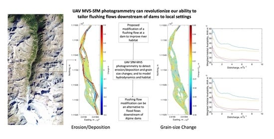
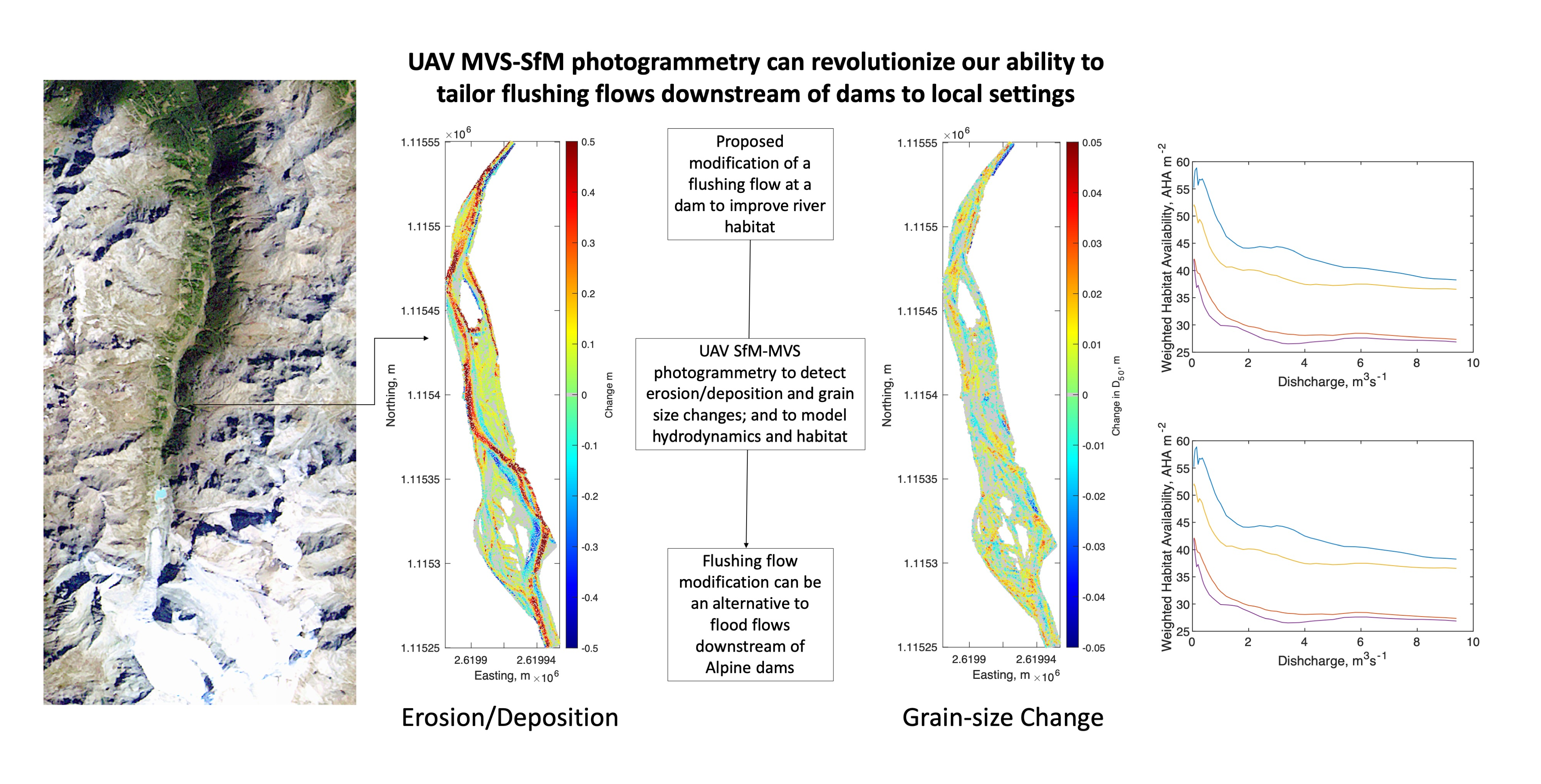
Combining UAV-Based SfM-MVS Photogrammetry with Conventional Monitoring to Set Environmental Flows: Modifying Dam Flushing Flows to Improve Alpine Stream Habitat

Abstract

Setting environmental flows downstream of hydropower dams is widely recognized as important, particularly in Alpine regions. However, the required flows are strongly influenced by the effects of the physical environment of the downstream river. Here, we show how unmanned aerial vehicle (UAV)-based structure-from-motion multiview stereo (SfM-MVS) photogrammetry allows for incorporation of such effects through determination of spatially distributed patterns of key physical parameters (e.g., bed shear stress, bed grain size) and how they condition available stream habitat. This is illustrated for a dam-impacted Alpine stream, testing whether modification of the dam’s annual flushing flow could achieve the desired downstream environmental improvement. In detail, we found that (1) flood peaks in the pilot study were larger than needed, (2) only a single flood peak was necessary, (3) sediment coarsening was likely being impacted by supply from nonregulated tributaries, often overlooked, and (4) a lower-magnitude but longer-duration rinsing flow after flushing is valuable for the system. These findings were enabled by the spatially rich geospatial datasets produced by UAV-based SfM-MVS photogrammetry. Both modeling of river erosion and deposition and river habitat may be revolutionized by these developments in remote sensing. However, it is combination with more traditional and temporarily rich monitoring that allows their full potential to be realized.

1. Introduction

There is a well-established linkage between streamflow regime and the availability of habitat for aquatic insects and fish (e.g., [1,2,3]). As many rivers and streams are also impacted upon by flow modifications, such as to supply drinking water, for irrigation, or for hydropower production, such modifications can also impact aquatic habitat [4]. Thus, the last 50 years or so saw the development and application of “environmental flows” or “e-flows” [5], which are designed to provide the water needed to restore ecological functions in human-modified streams [6,7,8]. Initially, e-flows focused on definition of the minimum flow that a river or stream needed to avoid negative impacts on instream fauna, notably fish. Wider research then showed that a focus on minimum flows is insufficient. An effective e-flow should also be determined with reference to the natural flow regime, notably including flow variability [4].

More recent work has recognized that aquatic habitat is not simply a function of the available flow [9], and this precludes setting an e-flow purely on the basis of hydrology. First, the ecological importance of any flow is conditioned by the shape of the stream bed, which impacts the way in which a given discharge produces spatial patterns of flow depth, velocity, and bed shear stress [10]. These hydraulic parameters have a direct impact upon the ability of aquatic organisms to live in certain parts of the stream bed, and this varies with the genus, the family, and sometimes individual species and subspecies [11,12,13,14,15,16]. Second, aquatic habitat is impacted upon by erosion and deposition, itself a product of bed shear stress, as well as rates of sediment supply to the stream. Too much erosion may lead to direct wash out of organisms, whilst too much deposition may lead to burial, thus making emergence of organisms from the stream bed difficult [17,18]. A complete lack of erosion can also lead to progressive accumulation of fine sediment on stream beds which may in due course lead to problems of colmation [19]. Erosion and deposition of sediment also have an important impact on organic matter availability and, hence, food sources [20,21,22,23]. It is for these reasons that e-flows have been extended to recognize the need also to address sediment-related issues or “sed-flows” [24,25]. Sed-flows are designed to manage flow and sediment in such a way that they improve the quality of the aquatic habitat available on the stream bed.

These two points pose a major challenge for incorporating habitat into the determination of e-flows. First, initial modeling attempts to quantify hydraulic controls on available aquatic habitat (hydraulic habitat modelling) were largely one-dimensional, assuming that the primary changes in habitat were from upstream to downstream [26]. However, it has become increasingly clear that habitat varies spatially within a cross-section, notably in meandering, anastomosing, and braiding streams. Thus, the determination of e-flows based on hydraulic habitat modeling should be two-dimensional [27,28,29] and able to capture the relatively small (meter-scale) gradients in hydraulics that seem to drive patterns of habitat suitability [30]. In turn, this requires spatially explicit datasets with the granularity to represent both local habitat availability (meter-scale) and the spatial extent to include all habitats that are available (10 s to 100 s of meters according to the stream being considered). Second, setting an e-flow, notably if this involves specifying flow variability, needs to be able to determine how the spatial patterns of habitat change through time. The resilience of a stream ecosystem is a function of the extent to which an organism can secure refuge in habitats that become suitable as discharge rises and then return to areas that were habitat suitable as discharge falls. Thus, we need tools that can predict where and to what degree zones outside those inundated at low river flows become suitable at higher river flows. Third, as it is now recognized that not only flow but also sediment can matter, it is vital to quantify and to model the spatial patterns of erosion and deposition to allow e-flows to also become sed-flows [25].

A number of data collection challenges and solutions follow. First, two-dimensional hydraulic habitat models begin by coupling digital topographic data to a depth-averaged solution of the Navier–Stokes equations for mass and momentum transfer [31]. Thus, they need high-precision, spatially distributed data on stream-bed topography. Traditionally, this has been acquired for inundated areas by wading the stream bed [32]. The advent of digital photogrammetry allowed stream-bed topography mapping using both two-medium photogrammetric methods [33,34] and coupled photogrammetry-image analysis techniques [35,36]. However, these methods were developed for conventional aerial imagery and, thus, restricted by the possible image resolution and the difficulties of achieving rapid aircraft mobilization. Aerial imagery can also be expensive for repeat, high-resolution survey of small areas. Airborne laser scanning is a valuable alternative solution (e.g., [37,38,39,40,41]), notably as green band data can more readily deal with effects of water (refraction, effects of turbidity) than photogrammetric applications; however, such systems are also expensive.

Second, most hydraulic habitat models commonly need at least some calibration because model simplifications (e.g., depth-averaging, estimation of the critical shear stress required for erosion/deposition) introduce parameters that are poorly known [42] but which may have a significant impact on model predictions (e.g., bed roughness parameters, the Shields parameter). If spatially distributed data on flow inundation and flow depths are available, they can be used to parameterize the flow model. Repetitive measurement of stream-bed topography can be used to calculate the spatial patterns of erosion and deposition and, hence, used to calibrate critical shear stresses. The importance of calibration points to the need for spatially distributed datasets relating to parameters in addition to topography.

Third, bed substrate is a critical determinant of available habitat for many aquatic organisms. In many rivers, notably gravel-bed rivers with a wide particle size range, substrate is spatially organized [43,44,45], and this organization can have an important impact on habitat [46]. Manual sampling of surface sedimentology is time-consuming, but it has been shown that the analysis of digital imagery can be used to provide spatially distributed data on sediment size [47,48,49,50,51,52,53,54,55]. Critical here is to be able to acquire imagery over the spatial extent of interest and with the granularity necessary for the associated algorithms to work.

The need for topography, calibration data, and spatially distributed grain-size data can all be addressed via harnessing geospatial technologies. In this paper, we aim to show how unmanned aerial vehicle (UAV)-based structure-from-motion multiview stereo (SfM-MVS) photogrammetric methods can deliver these data and, thus, enable much more effective monitoring of environmental flow and more intelligent proposals for future environmental flows. However, we also show that the real power of UAV-based photogrammetric methods is when they are combined with more traditional monitoring methods. We deliver this research through a focus on an environmental flow setting in a representative Alpine stream impacted by hydropower, the gravel-bedded Turtmänna river in southwest Switzerland, where a case for an environmental flow based upon an artificial clear water flood was made. Here, we follow a trial involving modification of the annual flushing of the associated storage dam to deliver downstream habitat improvements. In the next section, we present some background to the management options associated with evaluating hydropower impacts in Alpine streams. We then follow this with a methodology built around the datasets that UAV SfM-MVS photogrammetry can provide. We then present and discuss the results, separating them into a focus on (1) what conventional monitoring can show us, and then (2) how UAV-based SfM-MVS photogrammetry is critical to more effective monitoring and design of future environmental flows.

2. Environmental Flows in Alpine Streams: A Role for Geospatial Technologies

Hydropower infrastructure may disconnect sediment flux from upstream to downstream (notably in the case of dams) or modify it substantially where water is abstracted [56,57]. The result can be substantially negative, with direct and indirect impacts on stream ecosystems downstream of hydropower infrastructure (e.g., [25,58,59,60,61,62,63,64,65,66,67]). Although the need to set e-flows that guarantee a baseflow for downstream ecosystems is well established, it is now recognized that, downstream of dams, there can be, (a) loss of higher flows which may have an important biological function [4], (b) reduced supply of habitat-important gravel and coarser sediment [68,69], and (c) development of stream-bed colmation due to the accumulation of finer material [70] and reduced perturbation of the stream bed [71]. These impacts point to the need to factor sediment into e-flows [24,56] with the basic aim of increasing the percentage of gravel and coarser sediment on the stream bed.

There are three broad solutions. The first is the introduction of an artificial flood flow (i.e., an e-flow focused approach) which may serve to perturb the river bed downstream of a dam [72,73,74,75,76,77,78], provided the dam infrastructure allows such a release [79]. The magnitude of such a release needs to be established, and this is a complex process because of (1) the need to know the shape and the state of the stream bed throughout the river where habitat needs to be improved, as this will impact both the spatial patterns of bed shear stress and the critical bed shear stress needed for the onset of sediment transport, and (2) attenuation processes that will cause the flood wave to evolve with distance downstream. Both of these issues could be addressed through geospatial datasets especially if coupled with hydrodynamic models [29].

The second solution involves an artificial reintroduction of gravel and coarser sediment into a river downstream of a dam to replenish the system and aid in the restoration of river morphodynamics [80,81]. This is a relatively new approach and there have been very few studies that quantified the development of stream-bed morphology and granulometry as reintroduced sediment is reworked by the stream.

Third, many dams, especially smaller ones, need to be periodically flushed. These may be used to provide an artificial flood, but they need to be carefully designed [82,83]. A peak magnitude that is too high is likely to lead to equal mobility of sand and gravel and, therefore, not change the stream bed composition [82]. The flushing flow needs to be able to maintain the transport of fine sediment, which flushed from the dam and flushed from the stream bed, throughout the target length of river to avoid simply displacing the problem further downstream. They are of particular interest because flushing is a normal part of dam operation and, thus, it at least needs to minimize instream impacts. Questions remain as to whether or not it can be optimized to deliver benefits equivalent to an artificial flood flow. There are now some observations of the effects of flushing flows on stream habitat [84,85,86]; however, designing flushing flows remains a complex challenge and may have to be adaptive [83].

All three of these examples cause us to think about what environmental flow research could generalize. In all three cases, it is likely that environmental flows need to be set considering the specificity of the stream to which the flow is to be applied (e.g., slope, granulometry, morphology), as well as the objectives to be achieved as a result of the flow (e.g., physical objectives such as replenishing gravel habitat and breaking up stream-bed colmation or ecological objectives such as stimulating salmonid spawning). It is unlikely that transferable knowledge (e.g., that a river needs a certain discharge for a certain time) is likely to be forthcoming. For this reason, we developed a methodology that specifically integrates UAV-based SfM-MVS photogrammetric methods into setting environmental flows, which should be transferable and, hence, central to their setting in other geographical contexts.

3. Materials and Methods

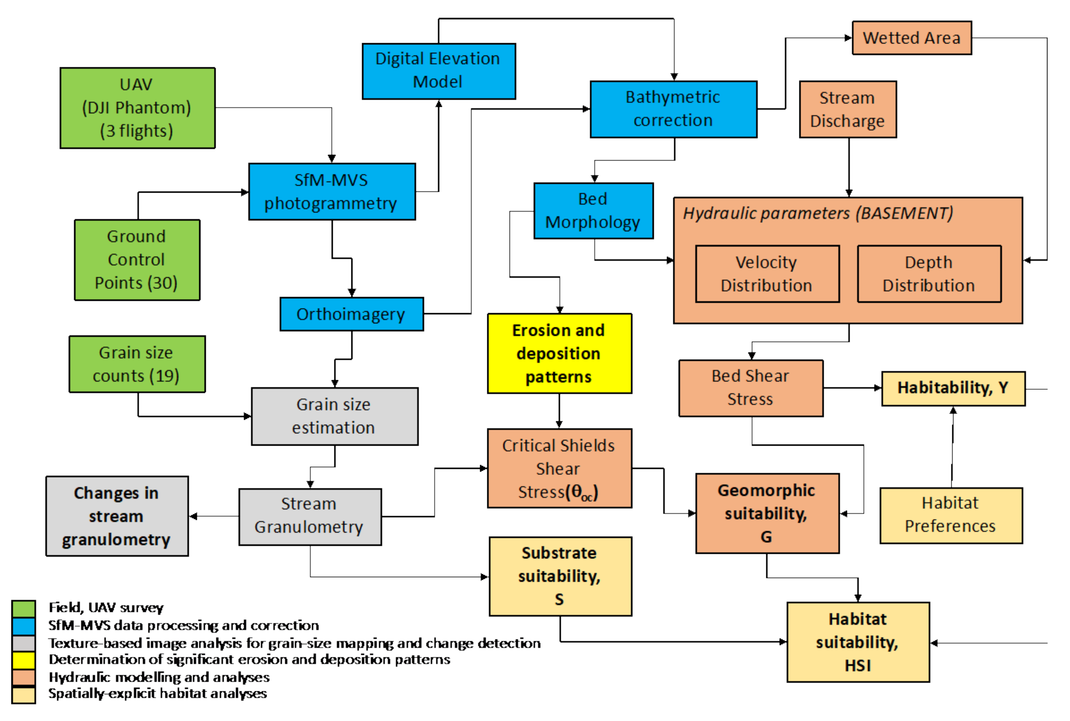
3.1. Methodological Approach

The overall methodology that we developed can be used to directly inform the design of environmental flows and to monitor the impact of environmental flows that might lead to different designs in the future. Here, our focus was on (1) monitoring a flushing flow in an Alpine stream that was modified with the aim of improving downstream aquatic habitat, and (2) designing improved flushing flows for future adoption. The modified flushing flow (MFF) that was monitored had the goal of improving the relative ratio of coarse sediment and fine sediment on the stream bed and of reducing stream-bed colmation. Such a flow should also give attention to how habitat availability changes during flushing flows, recognizing that too extreme a flow may reduce the rate of ecosystem recovery after flushing. This subsection explains the overall methodological approach (Figure 1). Subsequent subsections address each method in detail.

The approach we developed (Figure 1, green and blue) uses UAV-acquired imagery to derive digital elevation models (DEMs) and orthoimagery before and after the flushing flow using SfM-MVS photogrammetry [87]. Compared with traditional photogrammetric approaches, SfM-MVS differs in two important respects. First, “structure from motion” refers to the reconstruction of the position and orientation of the images with respect to the field of interest on the basis of a large number of automatically generated tie points (i.e., homologous point sets). Although the geometrical relations, notably the collinearity equations, are no different to those used in conventional analytical photogrammetry [88], the tie points are commonly viewed from very many images rather than just two (as is common in digital versions of analytical photogrammetry; [89]). By using techniques developed in computer vision (e.g., the scale-invariant feature transform, SIFT; [90]), this process can be automated, and imagery taken from very different angles and orientations with respect to the scene of interest can be used simultaneously even if the view of that scene is very different from each image. In theory, automation allows use of a large number of tie points with minimal effort and, thus, should improve the estimation of higher-order parameters, notably lens distortion. In turn, this makes it easier to use sensors that have poorly known or unstable internal geometry (as compared with traditional, calibrated photogrammetric sensors). Absolute position and orientation are then possible by using conventional ground control points, added during solution of the collinearity equations (which may also improve the solution [91,92]). Second, once there is an acceptable solution to the collinearity equations, “multiview stereo” methods are used to extract a dense cloud of three-dimensional (3D) point data from the imagery. Again, this differs from conventional digital analytical photogrammetry because the search for homologous point pairs uses computer vision methods such as SIFT, thereby allowing imagery from very different positions and orientations to be used.

Application of any kind of photogrammetric method to the quantification of river bathymetry is a challenge because water creates a two-medium problem. Two broad solutions exist. The first is image processing based upon the Beer–Lambert law [35,36] to estimate water depths for inundated zones which can then be incorporated into the digital topographic data-obtained dry zones. This works well for intermediate levels of turbidity in the water column, where the bed is still visible but loss of texture precludes the kinds of computer vision methods based on SIFT. If the turbidity is low enough for automated identification of homologous point sets, as in this study, then the problem can be treated as a two media photogrammetric problem (see [34,93] for the theoretical development). This is complicated for SfM-MVS analyses because, rather than each homologous point set being defined by two images, it is normally defined by very many. Each image has a specific relationship with a point on the stream bed, such that the refraction correction is more complex than the traditional case. Dietrich [94] developed a solution to this problem, which is used in this study, and this is explained below.

The key outputs from the SfM-MVS photogrammetry applied to the UAV data are (1) an image that is orthorectified to remove relief and sensor distortion, and (2) a point cloud that can be used to construct DEMs. Comparison of DEMs allows the determination of DEMs of difference that in our case could be used to determine the patterns of erosion and deposition due to the MFF (Figure 1, yellow). The DEMs are also used as input to a two-dimensional (2D) hydrodynamic model, BASEMENT (v2.8, [95]), which produces spatial patterns of velocity and depth from which bed shear stress can be determined (Figure 1, dark orange). A byproduct of the bathymetric correction is water depths and the extent of flow inundation, and these are used as calibration data for the hydrodynamic modeling. The hydrodynamic modeling is undertaken for a set of discharges from just smaller than a release equivalent to the Q₃₄₇ (the discharge for which 95% of flows are greater) through to a value greater than the maximum possible for the MFF as defined by the upstream hydropower-related infrastructure.

The hydraulic simulations are used in a spatially explicit hydraulic habitat model (Figure 1, light orange) for macroinvertebrates as a function of fuzzy analysis [25]. It estimates the following for the simulated discharges and for each location in the hydrodynamic model (Figure 1, light orange): (1) the habitability defined as a function of known macroinvertebrate preferences for bed shear stress [15], (2) the geomorphic suitability, defined as the risk of catastrophic erosion or deposition, and (3) the substrate suitability, a function of known macroinvertebrate preferences for certain substrates, largely reflecting different kinds of refuge preferences [96]. These three parameters are combined into a habitability suitability index (H) [25]. Following Gabbud et al. ([25]), the macroinvertebrates that are considered are defined by sampling for the case study stream.

The geomorphic suitability and the substrate suitability both rely on distributed data on stream granulometry that are also obtained via the UAV-based SfM-MVS analyses (Figure 1, gray). The orthoimages are combined with distributed Wolman ([97]) grid-by-number granulometric measurements to calibrate and to validate (via a split sample) a relationship between local image texture and grain size, which can then be applied to an entire orthoimage [47,48]. The associated stream granulometry can be transformed into the substrate suitability, as well as to produce a spatially distributed map of the critical Shields stress needed for erosion [98]. The Shields parameter that this requires has some uncertainty, especially because of processes such as grain interlocking and colmation, which can increase it by amounts that are poorly known a priori [19]. This problem is addressed using inverse modeling to calculate the uplift in the Shields parameter for sites that are estimated as eroding to a depth greater than the local grain size, using the maximum modeled shear stress during the MFF. Lastly, by applying the texture–grain size relationship before and after the MFF, it is possible to quantify grain-size changes.

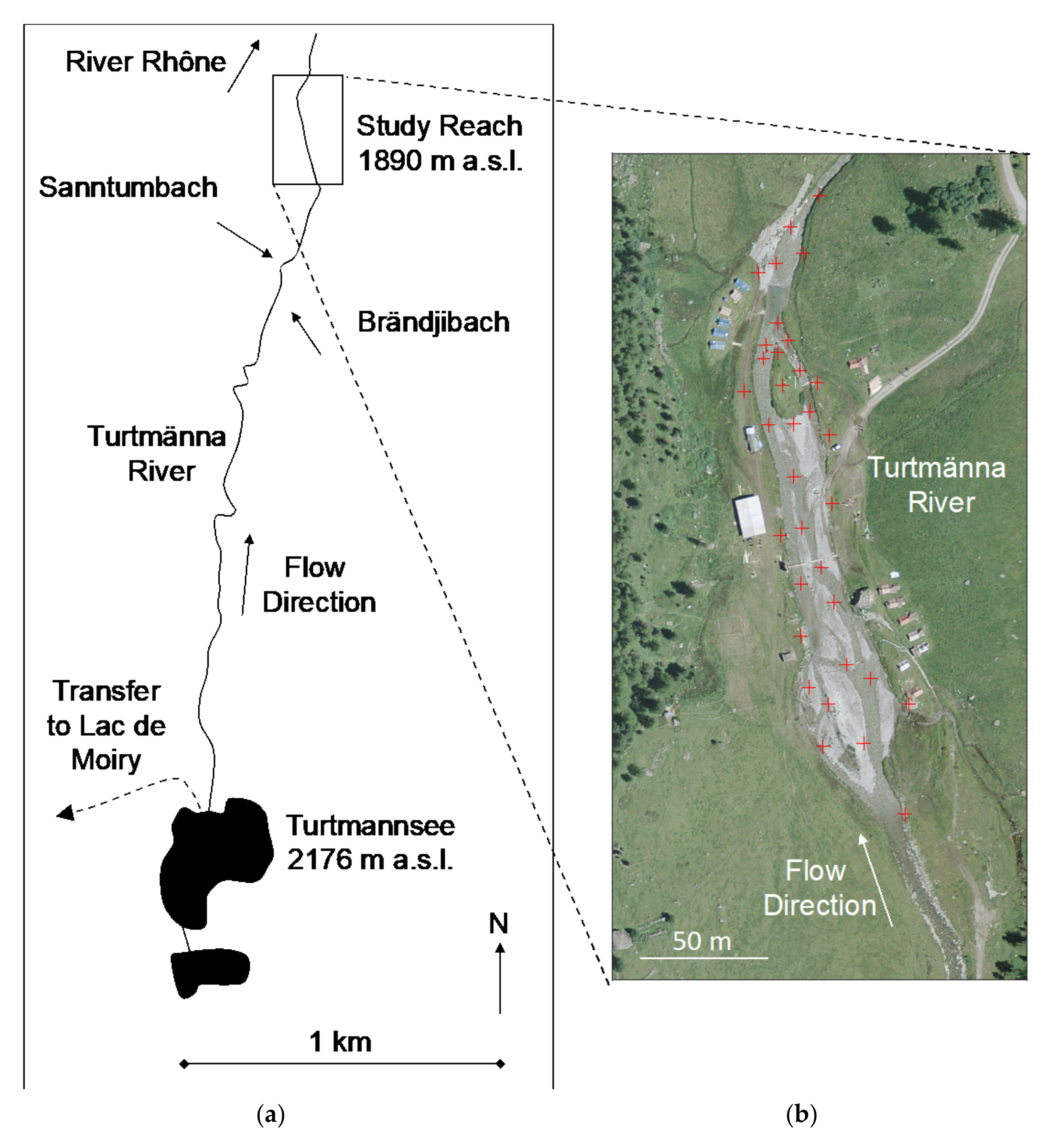
3.2. The Test Case: the Gravel-Bedded Turtmanna River, Switzerland

The focus of the research is the first unconfined reach of the 15 km long Turtmänna stream, at 1890 m above sea level and downstream of the Turtmannsee, the lower accumulation reservoir of two in the system (Figure 2a). The basin upstream of the Turtmannsee, ca. 29.6 km² in area, is glaciated and extends up to 4151 m above sea level. In a natural state, the stream would be classified as glacial [99]. Water is temporarily stored in the two reservoirs and transferred laterally to an adjacent valley and a larger reservoir (Lac de Moiry) for storage and eventual hydropower production.

The Turtmanna is predominantly confined until the start of the study reach where it develops a braided trace (Figure 2b). The remainder of the Turtmanna, until its junction with the Swiss River Rhône is mixed confined and braided. The reach studied here is representative of these braided zones. Such zones are of particular interest as research suggests that they contain diverse macroinvertebrate habitat at all flows [25]. It is located just below the tree line and is approximately 300 m long. It has a slope of 0.023 and comprises mixed sand, gravel, and cobble material with a mean D₅₀ of 0.019 and a mean D₈₄ of 0.044 m (before the MFF). Although it is only one reach of the Turtmänna, it is a critical one because (a) it is wide and braided, making it particularly valuable in terms of potential habitat, (b) it has one of the lowest valley slopes of all reaches of the Turtmanna and, thus, is likely to be one of the most sensitive to deposition, and (c) reaches further downstream are likely to be flushed naturally by nonregulated tributaries. The area upstream of the dam is 29.6 km²; the study reach has an additional 7.9 km² from the Sanntumbach and the Brändjibach (Figure 2a). Hydrologically, the Swiss Office fédéral de l’environnement, des forêts et du paysage ([100]) suggested a Q₃₄₇ of about 0.1 m³·s⁻¹ at the Turtmannsee. At present, there is no requirement to introduce a minimum flow downstream of the Turtmannsee; however, with 2 km of stream between the Turtmannsee and the reach studied here, there is some natural flow accrual to the Turtmänna notably from the Sanntumbach and the Brändjibach (3.8 km²), as well as from shallow aquifers. Given the relatively small area of unregulated river upstream (7.9 km²), this makes the study reach one of the most sensitive for minimizing flushing flow impacts as compared with further downstream. There are then a further 74.7 km² of nonregulated tributaries that join the Turtmänna downstream of the study reach and which could provide natural flood flows.

3.3. The Modified Flushing Flow (MFF)

Initially, a much larger and separate artificial flood (peak discharge of 15 m³·s⁻¹) was proposed as a suitable environmental flow for this stream, but this was challenged by local planning authorities given perceived concerns regarding risks to life and property. To avoid excessive sedimentation in the storage dam (Figure 2a), there is an annual flushing flow. Thus, this was modified by a consultancy company appointed by the operator of the Turtmänna hydropower system for testing in a trial on 8 October 2019. Before the trial, the flushing flow was designed only to rinse the basin. In the trial, the normal flushing flows were released in the morning as two peaks (Figure 3), and then a clear water flow designed to clean the stream bed of accumulated sediment was applied in the afternoon at two different flow intensities (Figure 3).

We collected field data before and after the MFF. The UAV flights (see below) were undertaken on 6 and 14 October 2019. The grain-size data were acquired on 7 October, the same day as macroinvertebrate samples. Macroinvertebrate sampling was also repeated on 15 October 2019. There was negligible precipitation before the study period and during it, and, aside from the MFF, the river appeared to have a largely constant discharge as confirmed by data from the Vispa river, immediately to the East of the Turtmanna, which had relatively steady discharge between 6 and 14 October 2019.

3.4. Conventional Monitoring

In addition to the UAV work schematized in Figure 1 and explained below, we were able to install two turbidity probes at the upstream (entry) and downstream (exit) of the reach. These reflect a more classical approach to establishing flushing flow impacts by allowing us to assess the extent to which the MFF resulted in a net loss of fine (i.e., suspended) sediment, as well as how this varied during the event. This was important as high turbidity during the event prevents the kind of within-event optical remote sensing using UAV that we describe below. The turbidity sensors were calibrated by sampling every 30 min at each sensor using a depth-averaging USDH-48 sampler. The volume of each sample was measured, and the sample was then filtered using preweighed 0.22 μm Millipore filters. The filter paper was dried at 105 °C, reweighed, and its mass divided by the filtrate volume to get the concentration. On this basis, we were able to develop calibration relationships between turbidity (Tu) and suspended sediment concentration (C).

C = 0.0153 Tu; R² = 96.5%, n = 9.

(1)

C = 0.0120 Tu; R² = 93.4%, n =7.

(2)

These relationships were applied to the time series of turbidity to obtain time series of suspended sediment concentration. The confidence limits (CI) were calculated as follows:

$$C{I}_o=\pm t\sqrt{\frac{\sum e^2}{n-2}\left[\frac{1}{n}+\frac{{\left(T_o-\overline{T}\right)}^2}{\sum T^2-n{\overline{T}}^2}\right]},$$

(3)

where t is Student’s t, defined here for one tail and n − 2 degrees of freedom; e is the set of residuals from the fits using equations (1, 2) and o indicates each data point in the time series of Tu. The discharge time series was multiplied by the C time series to give the instantaneous load (l). We calculated the uncertainty in the load from

$${\sigma }_l=\pm QCt{\left[{\left(\frac{{\sigma }_Q}{Q}\right)}^2+{\left(\frac{{\sigma }_C}{C}\right)}^2\right]}^{0.5};$$

(4)

however, as we had no information on the discharge uncertainty, we set it to zero. We also calculated the time cumulated load (L) each time T in the time series and its associated uncertainty, with the latter determined as

$${\sigma }_L=\pm t{\left[{\displaystyle \sum }_{i=1}^T{\sigma }_{QC}^i{}^2\right]}^{0.5}.$$

(5)

3.5. UAV Image Acquisition

On both 6 and 14 October, we acquired UAV images of the study reach (Figure 2) using a DJI Phantom 4 Pro with an onboard low-precision global positioning system (GPS). On each date, we used three flights, designed to reduce the degree of doming in the results [101]: two gridded flights, with an off-nadir angle of 10°, at average elevations of 30 m and 50 m above the ground surface, and overlaps of 65% and 80%, respectively, and an annular flight path 4° off-nadir also at 30 m above the ground surface. The UAV was flown close to the solar maximum with cloudy conditions to reduce problems of water surface reflection. As is common in flow regulated by a dam, the baseflow conditions during the UAV survey had negligible turbidity and the imagery had sufficient texture for the SfM-MVS photogrammetry throughout the inundated zone. In theory, with the camera used, this corresponds to a ground pixel resolution of 0.012 m. A total of 34 ground control points (GCPs comprising 0.60 m × 0.60 m black and white targets with reflective compact discs centered on the middle of the target) were installed across the study area (Figure 2b) [102] to improve the reliability of the image calibration [103], to improve the effectiveness of the MVS matching process, and to produce georeferenced data [87]. The GCPs were measured with a Trimble R10 differential GPS on both UAV flight dates. The Trimble base station was set up on the same fixed point on both dates, and data were transformed into the Swiss CH1903+/LV95 coordinate system using SwiPos-collected RINEX data from fixed, recording AGNES stations.

3.6. Image Calibration, Generation of Point Clouds and Orthoimagery, and Bathymetric Correction

UAV-acquired imagery was processed using the Pix4DMapper software following guidelines in [104]. UAV imagery was uploaded to the software, and, in a provisional stage, the UAV GPS coordinates were used to obtain an initial solution to the collinearity equations using bundle adjustments. This aided identification of the GCPs which were then used to improve the bundle adjustments. Research has shown that, even with many GCPs, SfM-MVS photogrammetric methods can struggle to recover the correct sensor internal geometry. Incorrect compensation for the focal distance, focal point position, and lens distortion can be common [101]. James et al. [101] suggested that this may be identified in significant correlations between these parameters. We checked this and there were no significant correlations in this case. The precision of the fitted GCPs (±0.018 m, pre MFF survey; ±0.018 m post MFF survey) was similar to the order of magnitude of the image resolution (0.012 m) suggesting that the bundle adjustment correctly identified the geometry of the system. Point clouds were then extracted with an average point space of 0.015 m and were interpolated to a resolution of 0.02 m. Orthoimages were produced at a resolution of 0.012 m. Initial comparison of the DEMs for the two dates revealed a systematic error manifest as a plane (rather than a dome). This is common with SfM-MVS photogrammetric methods even with correct flight plan design and GCPs [105]. The systematic error was removed following the recommendation of James et al. [104]. Points outside of the active river channel were identified and their corresponding elevations recorded. Point-by-point differences in these elevations were modeled to create an error surface and this was applied to the second DEM, thereby removing the systematic error.

To correct points that were inundated with water for the effects of refraction, we used multi-view correction [94], which is based upon the theory detailed in [34] and [93]. It was aided by the fact that the water depth was relatively shallow (mean 0.20 m; maximum 0.90 m), and there were few surface reflections and negligible suspended sediment concentrations during image acquisition, such that the stream bed could be seen throughout. To apply the multiview correction, for each date, inundated–dry boundaries were digitized from the orthoimage. Coordinate sets were then extracted from the point cloud using these boundaries and interpolated to create a water surface model. The boundaries were also used to extract point data to create a cloud of points known to be inundated. Subtraction of the altitude of each point from the water surface model allows an apparent depth to be assigned to each point. Pix4D parameters for image position, orientation, and internal geometry were then imported. For each point, a visibility analysis was undertaken to identify the images that might have contributed to the determination of that point. The possible real depth was then calculated for each image using a standard refractive index for water (1.337). This produced a set of real depths for each point and, following [93], the mean depth was calculated. The latter was then subtracted from the water surface model to give the corrected altitude for each point in the inundated zone point cloud. The inundated point cloud was then merged with those points that were dry to create a complete corrected point cloud. Given that the point density of this cloud was high, a simple triangulation-based interpolated was used to create a surface that was then interpolated onto a 0.012 m resolution DEM.

This process has two important byproducts for this research that assist with later hydrodynamic modeling: a classification of the study reach into wet and dry and point data on flow depth, both of which we could use to calibrate the hydrodynamic model. The two DEMs were also subtracted to quantify the erosion and deposition patterns due to the MFF. The results from the photogrammetric analysis, under the assumption that dry points and inundated points have the same quality, suggested a level of detection (after [89]) at the 95% confidence level of ±0.033 m, which falls between the mean D₅₀ and the mean D₈₄ of the study reach. This is an important criterion as an MFF should be capable of reworking at least the surface layer of inundated zones and, therefore, the design of the survey should allow for morphological changes to be determined that are comparable to the surface grain size.

3.7. Hydrodynamic Modeling

In order to produce estimates of velocity and depth and, hence, bed shear stress, for a range of different discharges, the 2D hydrodynamic model BASEMENT (v 2.7, [95]) was applied to the DEM collected on 6 October 2019. Its choice and manner of application followed [25]. BASEMENT solves the depth-averaged Navier–Stokes equations for mass and momentum conservation on a finite element mesh. The Reynolds decomposition uses a zero-order turbulence model which requires specification of an eddy viscosity which we treat as a calibration parameter. A quadratic friction law with a Manning-type relationship was used to define the boundary shear stress condition. For computational reasons, the 6 October DEM was resampled to a 0.5 m resolution and a plug-in for the software QGIS, BASEmesh, was used to create the finite element model from the resampled data. An exact Riemann solver was used for model solution with time steps set implicitly to satisfy the Courant–Friedrichs–Lewy condition. The downstream boundary used a depth–discharge relationship based upon the Manning equation. Following [25], this boundary was set downstream of the study reach such that it had no impact upon the area of interest. In all model runs, a steady discharge was applied at the upstream section and the model run to steady state, such that the mass balance error (the difference between mass inflow rate and mass outflow rate) was less than 0.5%.

We followed Gabbud et al. [25] and undertook initial testing of model parameters to identify the most sensitive. These tests found that turbulent viscosity and friction slope at the downstream end of the simulation had negligible impact upon model predictions, and that Manning’s n was the most important parameter. We had no discharge information at the same time as the flights (for logistical reasons) and, thus, we also included discharge as a calibration parameter (as did [25]). With the grain size mapping described below, we could have estimated spatially distributed values of n. However, n is likely to be an effective parameter in this case (the values needed to optimize the model may be different to those measured from grain size, because other processes are being represented in the model; see [42]). Furthermore, studies of 2D hydrodynamic models suggest negligible relative sensitivity to n values as compared with their one-dimensional (1D) counterparts [106,107]. Thus, we undertook simulations with uniform values of n within the range 0.045 to 0.060 following experience in streams with similar slopes and grain sizes, close to the study area [25,108]. We simulated three discharge values, 0.20 m³·s⁻¹, 0.25 m³·s⁻¹, and 0.30 m³·s⁻¹. These were chosen on the basis of qualitative observations of model predictions whereby discharges outside of the range defined by these values resulted in severe underprediction or severe overprediction of inundation during the flights on 6 October.

Each simulation was evaluated qualitatively by visual comparison of predicted inundation and the inundation extent digitized for the bathymetric correction. We did not undertake a quantitative comparison here as we found that the secondary branches of the stream (Figure 2) were either not inundated when they should be or inundated when they should not be, thus providing a very sensitive indicator of optimum parameters for simulation. We did, however, undertake quantitative comparison of the water depths estimated during the bathymetric correction with those modeled (

Table 1. Summary of model simulations to optimize discharge (Q) and n; inundation indicates qualitative comparison of inundated branches with predictions (OK indicates all branches predicted as wet were observed as wet), slope of the line of the reduce major axis (RMA) fitted line for measured and predicted depths to quantify systematic error, and correlation between measured and predicted depths to quantify precision.

		Inundation			Slope			Correlation
n/Q (m3·s−1)	0.20	0.25	0.30	0.20	0.25	0.30	0.20	0.25	0.30
0.045			OK			0.876			0.870
0.050	X		OK	0.943		0.870	0.862		0.871
0.055	X	OK		0.937	0.897		0.863	0.869
0.060		OK			0.891			0.870
0.070		OK			0.878			0.871

). We recognized two kinds of error: (1) a systematic error, which we estimated using a reduce major axis (RMA) regression slope given that both the measured and the modeled depth could be systematically incorrect, reflected in deviations of the root-mean-square (RMS) slope from the line of equality, and (2) correlation, a measure of the precision of the model.

Initial simulations suggested that a secondary branch was only inundated if Q > 0.20 m³·s⁻¹, despite the latter value giving the slope values closest to 1 and, hence, the smallest systematic error (Table 1). We then found for Q > 0.20 m³·s⁻¹ that, despite a weak inverse tendency for less systematic error (i.e., slope values closer to 1) to have lower correlations, the differences were small, notably in response to changes in n. Increasing Q to 0.30 m³·s⁻¹ reduced the slope further; thus, we settled on Q = 0.25 m³·s⁻¹ and n = 0.06. Lastly, to investigate what happens with an even higher value of n, we simulated n = 0.07 at Q = 0.25 m³·s⁻¹. This produced a more marked slope reduction and only a small correlation improvement (Table 1). Thus, we used Q = 0.25 m³·s⁻¹ and n = 0.06 as our (weakly) optimal solution. Once the model was optimized, discharges were simulated as follows:

• From 0.05 m³·s⁻¹ to 0.10 m³·s⁻¹, we simulated every 0.01 m³·s⁻¹;
• From 0.10 m³·s⁻¹ to 0.50 m³·s⁻¹, we simulated every 0.05 m³·s⁻¹;
• From 0.50 m³·s⁻¹ to 1.00 m³·s⁻¹, we simulated every 0.10 m³·s⁻¹;
• From 1.00 m³·s⁻¹ to 5.00 m³·s⁻¹, we simulated every 0.20 m³·s⁻¹;
• From 5.00 m³·s⁻¹ to 9.40 m³·s⁻¹, we simulated every 0.40 m³·s⁻¹.

The highest discharge simulated (9.40 m³·s⁻¹) was designed to extend to just higher than the maximum planned release (9.00 m³·s⁻¹, Figure 3) considering that we estimated the baseflow to be around 0.25 m³·s⁻¹. The discharge intervals were simulated, reflecting the fact that small changes in discharge can lead to rapid changes in available habitat (e.g., [25]).

3.8. Quantification of the Likelihood of Bed Break Up

As a major goal of the MFF was the elimination of colmation and the breakup of the stream bed to release fines and to re-aerate the subsurface, we aimed to quantify the likelihood of scour. Evidence suggests that this scour depth should be sufficient to open up interstices between larger particles to allow fine sediment to escape [19]. For each simulation, and for each point in the domain, we quantified the critical shear stress (τ_oc) using the Shields formation [98].

$${\tau }_{oc}={\theta }_c\left({\rho }_s-{\rho }_w\right)g{D}_{50},$$

(6)

where ${\theta }_c$ is the critical value of the Shields parameter, ρ is the density of s (sediment) and w (water), g is gravity, and D₅₀ is the median grain size determined via orthoimage analysis (see below). Above a critical value of grain size, ${\theta }_c$ is thought to be constant [98]. If the grain size is uniform, ${\theta }_c$ is generally taken as 0.06. However, research suggests that if the grain-size is mixed, as in this case, the necessary value of ${\theta }_c$ may be as high as 0.1 and even higher if the bed is highly imbricated or armored [109,110,111] or colmated [19]. The problem is that the extent of upscaling of ${\theta }_c$ that is needed is not only poorly known, but also likely to be spatially (as a function of grain size) and temporally variable (because lower flows can still lead to grain sorting and imbrication and the development of colmation). We addressed this problem using an inverse method. We spatially distributed data on grain size (D₅₀ in (6)) at baseflow and before the event from the image analysis (Figure 1; see Section 3.9). The hydrodynamic modeling gives us bed shear stress at baseflow (τ_o). Our observations suggest that, at baseflow, there was no sediment transport. Hence, we can determine the uplift of the value of ${\theta }_c$ in Equation (6) necessary for there to be no sediment transport in the base flow simulation; that is, we can parameterise the potential effects of armoring and colmation by using the “no sediment transport condition” and the remotely sensed grain-size estimates. The analysis results in a spatially variable value of ${\theta }_c$ which also reflects evidence in the orthoimagery and grain-size maps (see explanation and Figure 4 below) that there are zones of gravel and cobble material with little fine sediment and where armoring is a possibility, as well as drapes of fine sediment which are unlikely to need any uplift in ${\theta }_c$. It should be emphasized here that this approach would yield the required minimum values of the uplift in ${\theta }_c$.

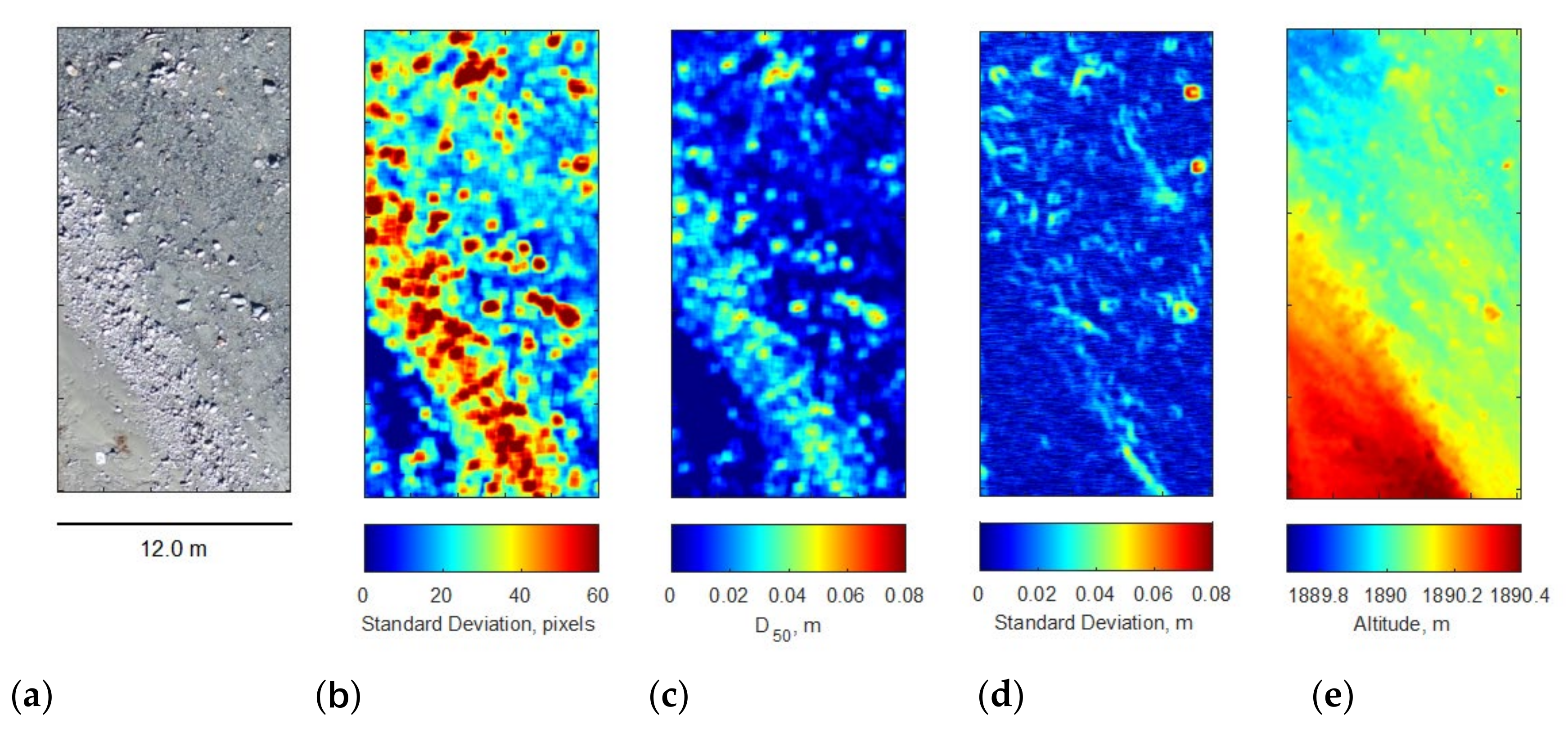
3.9. Grain-Size Estimation

Figure 1 showed how the grain size estimation fitted into the workflow for the UAV-based research, using calibration of the texture signal derived from the orthoimagery. We undertook 19 Wolman [97] grid-by-number samples on 6 October 2019. Each sample was based upon a 1.1 m × 1.1 m quadrat with 10 × 10 cross strings to identify 100 clasts for sampling on a 1 m × 1 m grid. If two crosses fell on the same grain, the grain was counted only once and the sample size was reduced. Grain b-axes were measured using calipers and the grid D₅₀ was estimated. The Wolman grids were located randomly across the active part of the study area and the corners of each grid were measured using the differential GPS (dGPS). The dGPS points were then used to identify the corresponding zones in the orthoimage and, following [47,48], the texture of the image (here taken as the local standard deviation of the image corresponding to the quadrat) was calculated (e.g., Figure 4b). Use of the orthoimagery is preferable to use of DEM (e.g., Figure 4e) data because, as with any photogrammetric method, the resolution that can be acquired with the former is higher than the latter. This is reflected in the higher information content in the image standard deviations (Figure 4b) as compared with the altitude standard deviations (Figure 4e). Furthermore, there are scales of variability in topography that do not relate to grain size (e.g., grain organization, larger scales of river morphology), which can lead to misleading estimates of texture. The main problem with use of the image texture as compared with DEM data is that the texture of inundated zones may be different to non-inundated zones. However, we found that converting the orthoimage to grayscale eliminated the differences between inundated and dry samples, although our experience elsewhere has shown that this is not always the case and that inundated and dry zones may need to be treated separately to avoid bias in grain-size estimates in different zones of the river. We split the Wolman grid data into two, with 10 grids used for calibration. As expected given the work of Carbonneau et al. [47,48], we found a linear relationship between texture and D₅₀, and ordinary least squares regression was appropriate. When we applied this to the nine unused grids, the mean error was −0.002 m and the standard deviation of error was ±0.005 m. Centered on each node used in the BASEMENT model, we extracted the related 1 m × 1 m grid from the orthoimagery, calculated the associated standard deviation, and then applied the calibration relationship. As this was based upon simple linear ordinary least squares regression, we could also calculate confidence intervals for each estimated grain size. The potential of this approach to grain-size estimation is shown in Figure 4, with median grain size estimates (Figure 4c) for a subsection of an orthoimage (Figure 4a).

We were not able to collect grain size data after the MFF and, thus, we needed to be able to apply the calibration relationship developed for data from 6 October. However, lighting conditions were slightly different on the two days. Therefore, in order to quantify how the grain size changed, we identified the zone inundated as predicted by applying BASEMENT to the highest simulated discharge. We then identified areas that were not inundated and the scaling and stretching needed to map the 14 October non-inundated areas onto the 6 October non-inundated areas. We then applied this scaling and stretching to the full 14 October image and applied the 6 October calibration to the same BASEMENT nodes. We also identified 28 estimates of grain size for the two dates from non-inundated areas that were not used for the scaling and, hence, where there should be no grain size changes between dates. The associated mean error was −0.004 m and standard deviation of error was ±0.008 m.

With these analyses, we could then determine (1) a digital grain-size difference (DGD) map for the median grain size, and (2) an associated level of detection limit for grain-size changes equivalent to that for erosion/deposition changes in a DEM of difference. With a standard deviation of error for the validation sites of ±0.008 m, at the 95% confidence limit, this was ±0.016 m.

3.10. Hydraulic Habitat Modeling

In the final element of the analysis (Figure 1), we undertook fuzzy habitat modeling using the method reported in detail in [25]. This paper contains a summary of this method and highlights one important difference. A fuzzy logic approach was used [112,113,114,115,116,117,118,119] with the goal of estimating the relationship between discharge and habitat availability for different families of macroinvertebrates (see also [112,113,114,117,118,119]). Evaluating the suitability of habitat has three elements. The first two follow [25]: (1) the habitability (Y) is estimated to represent the ability of an organism to remain in a particular part of a stream, a function of the local bed shear stress; increases in shear stress can lead to density-independent loss of benthic macroinvertebrates ([11]), dependent on the genus, the family, and sometimes individual species and sub-species (e.g., [12,14,15,16]); (2) the geomorphic suitability (G) is taken to be a measure of the extent to which a particular part of a stream is prone to erosion or deposition (after [25]). In Gabbud et al. [25], G was calculated from modeled shear stresses coupled to an assumed characteristic grain size to estimate the critical Shields stress. Here, we spatially distributed grain-size estimates derived from UAV imagery, and, unlike in [25], we also derived a spatially distributed estimate of the critical shear stress required for sediment transport. We assumed that there was an intermediate value of shear stress that was optimal: some scour would reduce colmation and re-oxygenate the stream bed; too much scour would lead to complete loss of organic matter and, hence, food sources and eventual habitat wash out; too much deposition would lead to burial.

In this paper, we introduced a third parameter, substrate suitability (S), as different macroinvertebrates have different substrate preferences [120,121]. These may relate to the different ways in which macroinvertebrates seek refuge in response to perturbation or predation [122,123,124,125,126]. Tachet et al. [96] provided broad substrate preferences for European macroinvertebrate families, allowing grain size to be transformed into a substrate suitability S.

For the three parameters Y, G, and S, following [25], we defined three classes: poor, medium, and good. The boundaries of these classes were fuzzy, defined by estimated uncertainties in both the value of the parameter being classed and the membership of that value in the three classes. Thus, any one location could be a member of more than one class (of Y, G, or S) with the total membership of all classes being 1. The classes of Y, G, and S were combined using a product operation rule [127] to define the degree of fulfilment of each habitat class. These were defuzzified onto a single dimensionless scale, H, varying from 0 (where all classes of Y, G, and S were 100% poor) to 1 (where all classes of Y, G, and S are good). H did not have units as it was based upon classification. These steps are explained in more detail in [25] and the membership rules are shown in

Table 2. Definitions of rules for good, medium (“med”), and poor habitat for habitability (Y) in terms of shear stress and substrate suitability (S) as a function of median diameter (D₅₀). The habitat classes have two sets of data, 1 and 2, for poor and medium habitat, as these classes exist both sides of the good habitat class. For example, for Limnephilidae, shear stress is labeled as poor between 0 and 0.010 N·m⁻² (set 1) and between 1.09 N·m⁻² and infinity (set 2). The shear stress rules were the same as those used in Gabbud et al. [25].

	Poor Min (1)	Poor Max (1)	Poor Min (2)	Poor Max (2)	Med Min (1)	Med Max (1)	Med Min (2)	Med Max (2)	Good Min	Good Max
Shear Stress, Nm−2
Limneph.	0	0.010	1.09	∞	0.010	0.07	0.529	1.09	0.07	0.529
Baetidae	0	0.118	11.27	∞	0.118	0.393	6.34	11.27	0.393	6.34
Chironim.	0	0.077	4.48	∞	0.077	0.083	0.118	4.48	0.083	0.118
Perlodidae	0	0.083	6.34	∞	0.083	0.118	1.59	6.34	0.118	1.59
D50, m
Limneph.	0	0.001	0.2	∞	0.001	0.01	0.1	0.2	0.01	0.1
Baetidae	0	0.002	0.5	∞	0.002	0.02	0.2	0.5	0.02	0.2
Chironim.	0	0.0005	0.2	∞	0.0005	0.01	0.1	0.2	0.01	0.1
Perlodidae	0	0.01	0.5	∞	0.01	0.02	0.2	0.5	0.02	0.2

.

The values of habitat suitability, H, are spatially referenced; thus, habitat can be mapped for any value of simulated discharge. The habitat maps are valuable in showing how habitat suitability moves in space as discharge changes, important in braided mountain streams as zones that are unsuitable at low flow may become suitable at high flow and vice versa. The usability of changing habitat is ultimately dependent on the ability of an organism to access it (a function of the capacity of an individual to disperse, the displacement distance needed to access better habitat, and the rate at which the habitat is being displaced). Our analyses did not consider this issue. We also calculated two reach-scale habitat indices (after [25]): (1) a measure of total habitat, the sum of all H values, which we labeled absolute habitat availability (AHA); (2) a measure of habitat quality, equivalent to a weighted usable area [128]), taken as the AHA divided by the area that was inundated, which we labeled weighted habitat availability (WHA) [129,130]. Note that AHA is a relative measure that can be compared for a site at different times or for different organisms; that is, if the spatial resolution changes, then the AHA changes.

3.11. Biological Sampling, Habitability, and Substrate Suitability Rules

A small amount of biological sampling was undertaken to identify the dominant insect families present in the stream. Our primary aim was to use these samples to identify which families to model (following [25]); however, it also gave us a basic opportunity to quantify how insect populations responded to the flood. We used the approach described in [67]. Insects were sampled using 30 s kick samples and a kick sampler with a 0.25 m × 0.25 m net and mesh size of 1 mm. Two replicates were obtained from each of three substrates (sand, gravel, and cobbles and coarser). The six sample sites were recorded using differential GPS such that we could sample the day before the flood and then reoccupy adjacent sites to each initial sampling site one week after the flood. In all cases, insects were sorted and stored in 97% strength ethanol. They were then sorted under magnification using [96] to the family level.

Four families were found to be most prevalent: Chironimidae, Limnephilidae, Baetidae, and Perlodidae. For each of these, we used the data in [15] to establish shear-stress based rules for habitability (Y) and data in [96] to established grain-size based rules for substrate suitability (S) (Table 2).

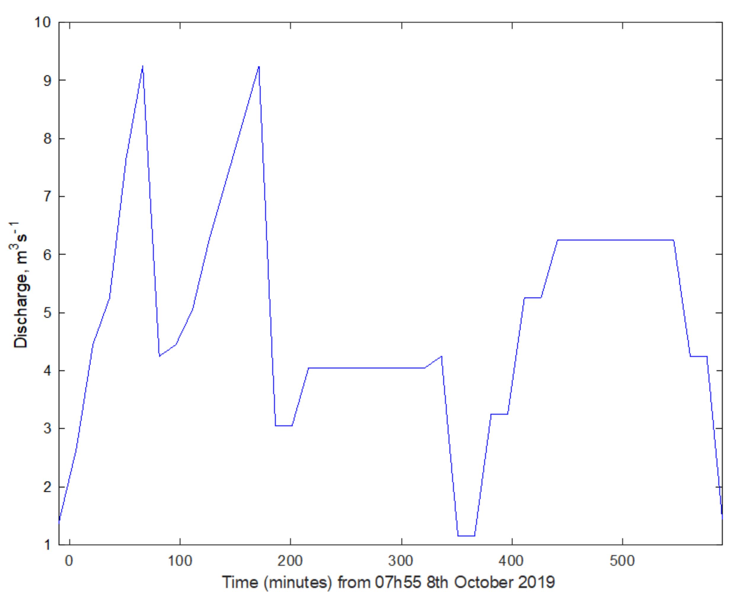
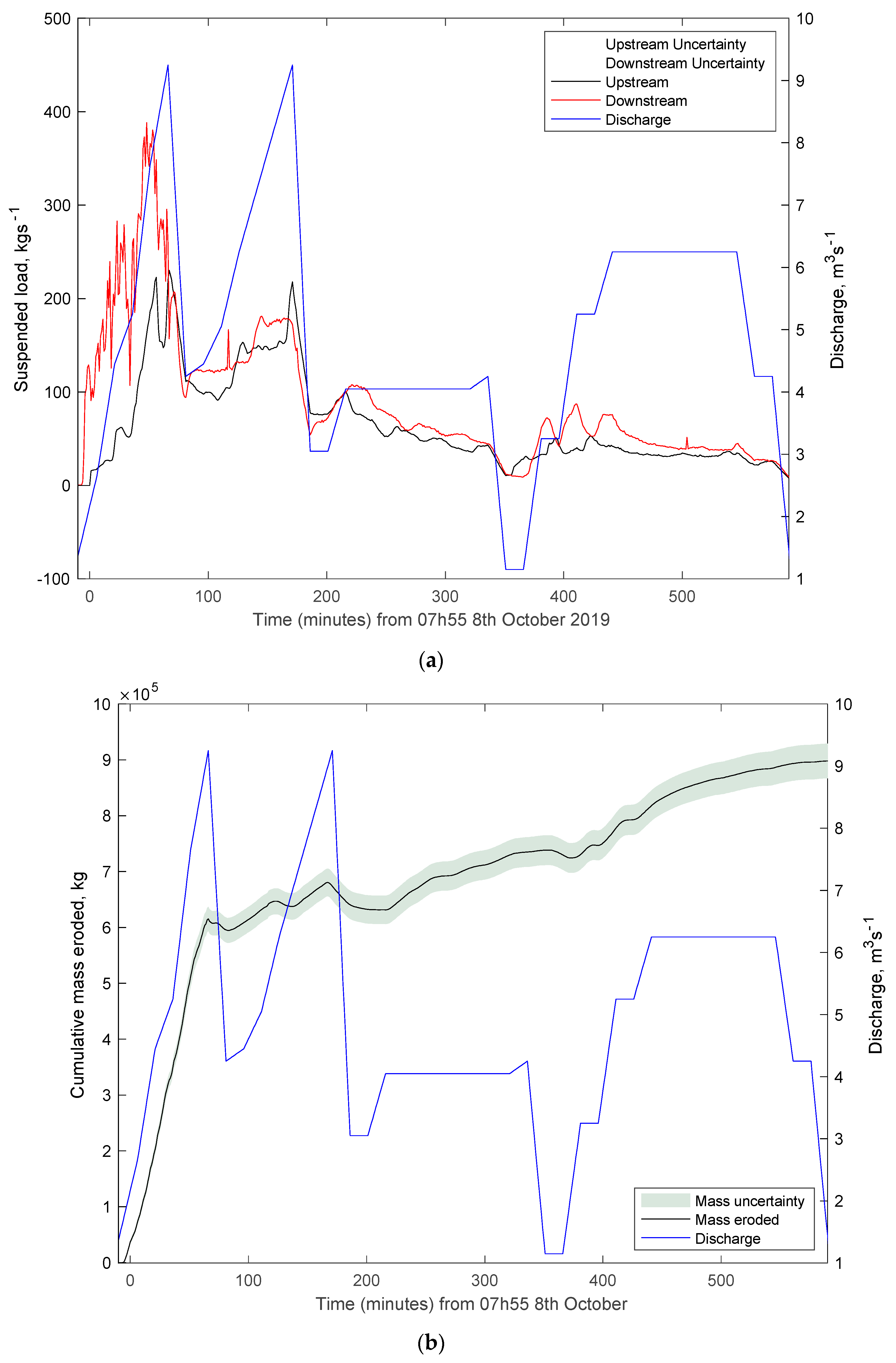
4. Discharge, Instantaneous Load, Cumulative Load, and Biological Monitoring

This section presents and discusses the results from a traditional monitoring approach applied to the MFF. It allows us to show in Section 5 how the methodology outlined in Figure 1 not only explained the results from this monitoring but also allowed us to identify unexpected effects of the MFF and then to redesign the MFF in a way that increased its potential ecosystem benefits.

4.1. Results

The time series of discharge and suspended sediment load, upstream and downstream of the study reach, during and after the MFF (Figure 5a) show that, in general, the downstream sediment load was higher than at the upstream site, implying a net loss of fine sediment during the event. During the first 90 min of the event and the first MFF peak (MFFa), the quantity of downstream exported sediment (i) rose more rapidly and to a higher level than the quantity of upstream supplied sediment, and (ii) rose as soon as there was an increase in discharge. The upstream sediment supply started to rise about 30 min after the arrival of the discharge wave. There was a 2 km distance between the study reach and the upstream dam (Figure 2a), suggesting a difference in travel times between the water wave and sediment wave of 15 min per km. There was a 10 min delay of the suspended sediment wave in crossing the 300 m long reach (Figure 5a), i.e., about 30 min per km, somewhat slower but probably reflecting the reduced slope of the study reach.

After the first discharge peak, the sediment loads both upstream and downstream declined. The response of both upstream and downstream sites to the second MFF peak (MFFb) was less marked. There is evidence of a delay between the downstream and the upstream changes in load, with the upstream site leading the downstream site in MFFb, the opposite of MFFa (e.g., between 130 min and 170 min into the MFF). This delay was seen later in the experiment, between 360 min and 460 min, where both upstream and downstream sites had three peaks in load, the upstream sites again occurring before the downstream sites. The delay was around 10 min. The onset of the clear water releases (CW) from 200 min maintained higher instantaneous loads downstream as compared with upstream (Figure 5a). There was a net loss of suspended sediment during the flood but most of this was during the first 70 min of the experiment (Figure 5b). Then, the rate of increase of sediment loss slowed. Between MFFb and the first clear water release (CWa), as well as between CWa and the second clearwater release (CWb), the cumulative mass eroded declined. Other than for these two periods, the cumulative mass increased until the end of the experiment.

Table 3. Numbers of individuals measured by family and substrate before and after the trial modified flushing flow (MFF).

	Sand	Gravel	Cobbles and Coarser	Total by Family
		Before the MFF
Chironimidae	16	13	8	37
Limnephilidae	6	28	25	59
Baetidae	19	58	249	326
Perlodidae	6	31	60	97
Total by substrate	47	130	342
	After the MFF
Chironimidae	1	1	3	5
Limnephilidae	3	6	71	80
Baetidae	0	35	159	194
Perlodidae	0	13	72	85
Total by substrate	4	55	305

shows the results of the sampling of aquatic insects for the four most important families recorded. The results before the flood, notably the distribution of families between substrate classes, reflect expected species preferences [96]. The decline in insects due to the flood was proportionally greater for sand than gravel and for gravel than cobbles and boulders. All families declined, with the greatest decline by proportion in the family preferring the finest substrates (Chironomidae). These four families are used in the hydraulic modeling below.

4.2. Discussion

The primary conclusion from these data is that the entire event resulted in a net loss of fine sediment from the study reach, approaching 900 tons in total (Figure 5b). This was despite the flushing flow itself being highly loaded with sediment (Figure 5a, upstream curve). Approximately two-thirds of this loss occurred during the first phase of the MFF (Figure 5b), before the arrival of the sediment released from the dam during flushing (Figure 5a). The second flushing flow (MFFb) and the two clearwater flows (CWa and CWb) continued the removal of fine sediment (Figure 5b) at a lower rate, confirming the observations of others regarding the importance of sustained high flows after flushing in preventing deposition of fine sediment and securing its continued removal [84,131,132].

Evidence suggested that both the arrival of flushed sediment from upstream and the translation of sediment through the reach were delayed by 15 min per km and 30 min per km, respectively, and this is likely to reflect a long-established kinematic effect [133]. Suspended waves travel more slowly than water waves due to a reduction in turbulence intensity with height above the stream bed and, hence, a reduction in suspended sediment concentration. Velocity increases with height above the stream bed to reach a maximum just below the water surface. Thus, sediment is suspended at elevations above the stream bed with lower flow velocity than the velocity profile mean, and suspended sediment waves move more slowly than flood waves [133]. Unlike in other studies [86], this means that the initial effect of the MFF is removal of sediment from, rather than deposition of fine sediment in the stream bed. If our reach was closer to the dam, then we might have also seen initial deposition, although this would have depended upon stream competence to transport sediment, as well as the duration of flushing. Such distance effects were observed in similar settings [131,134]. The initial evidence, however, suggests that the first flushing flow peak (MFFa) led to substantial removal of fine sediment from the reach studied here.

The removal of fine sediment (Figure 5) was reflected in the biological data. The proportional decline in the number of insects was greatest on the finer substrates (Table 2). Families that preferred finer sediment (see [96]) were impacted more than those that preferred coarser sediment (Table 2), e.g., Baetidae, with insects that commonly respond to perturbation by drift or hiding between larger clasts.

Whilst these results may support the use of MFFs in this situation to remove accumulated fine sediment, a number of limitations arise in relation to this monitoring approach. First, the monitoring reveals the net loss of suspended sediment associated with the MFF. It is quite possible that the MFF only removed easily transportable but relatively thick sand deposits. Fine sediment that infiltrated between gravels and coarser particles may not have been transported. Whilst it is well established that fine sediment can be flushed from the bed of a stream in the absence of gravel transport [82,135], this does not necessarily apply to anything more than the surface layer of gravel particles. Flushing deeper into the bed requires some gravel transport but not so much that there is substantial gravel loss [82]. Similarly, net fine sediment loss may also hide the formation of new zones of deposited fine sediment. Assessing the effects of the MFF needs spatially distributed data on the depths of bed reworking, the patterns of sediment deposition, and changes in the surface size distribution of sediments.

Second, the monitoring provides no hydraulic information that might allow the design of the MFF to be improved. Whilst testing different flushing flows might allow optimization (e.g., [83]), in order to capture the full set of impacts of each option tested, substantial resources would need to be invested in multiple trials. It is highly likely that the relationship between the discharge associated with an MFF and hydraulic parameters, notably shear stress, is strongly conditioned by local factors (e.g., reach slope, initial channel pattern, bed roughness) [77,134], which would make it difficult to generalize MFF trials beyond the system to which they have been applied. Kondolf and Wilcock [82] noted that a flushing flow must be designed to maximize sand transport but minimize gravel transport, whereas the optimal ratio is likely to occur over a very narrow range of shear stresses. These vary spatially, notably in multithread or braided mountain streams [10]. Equally, once the flushing flow peak has passed, it is important to determine for how long a dilution flow needs to be maintained and at what magnitude so as to avoid excessive waste of water. Again, this requires either expensive trials or hydrodynamic calculations that are sensitive to how the spatial patterns of bed shear stress change as a function of discharge.

The final element that was not considered in these analyses is how the habitat availability changed as a function of discharge. It is well established that flushing flows can have negative habitat consequences [84,86,131,132]. Some of this can result from the negative consequences of sediment deposition [84,131,132,136], some of it from the loss of suitable habitat, and some of it from enforced drift [137,138]. These observations suggest a need to understand how habitat evolves during the MFF, so as to factor at least a partial consideration of ecological function into decision-making.

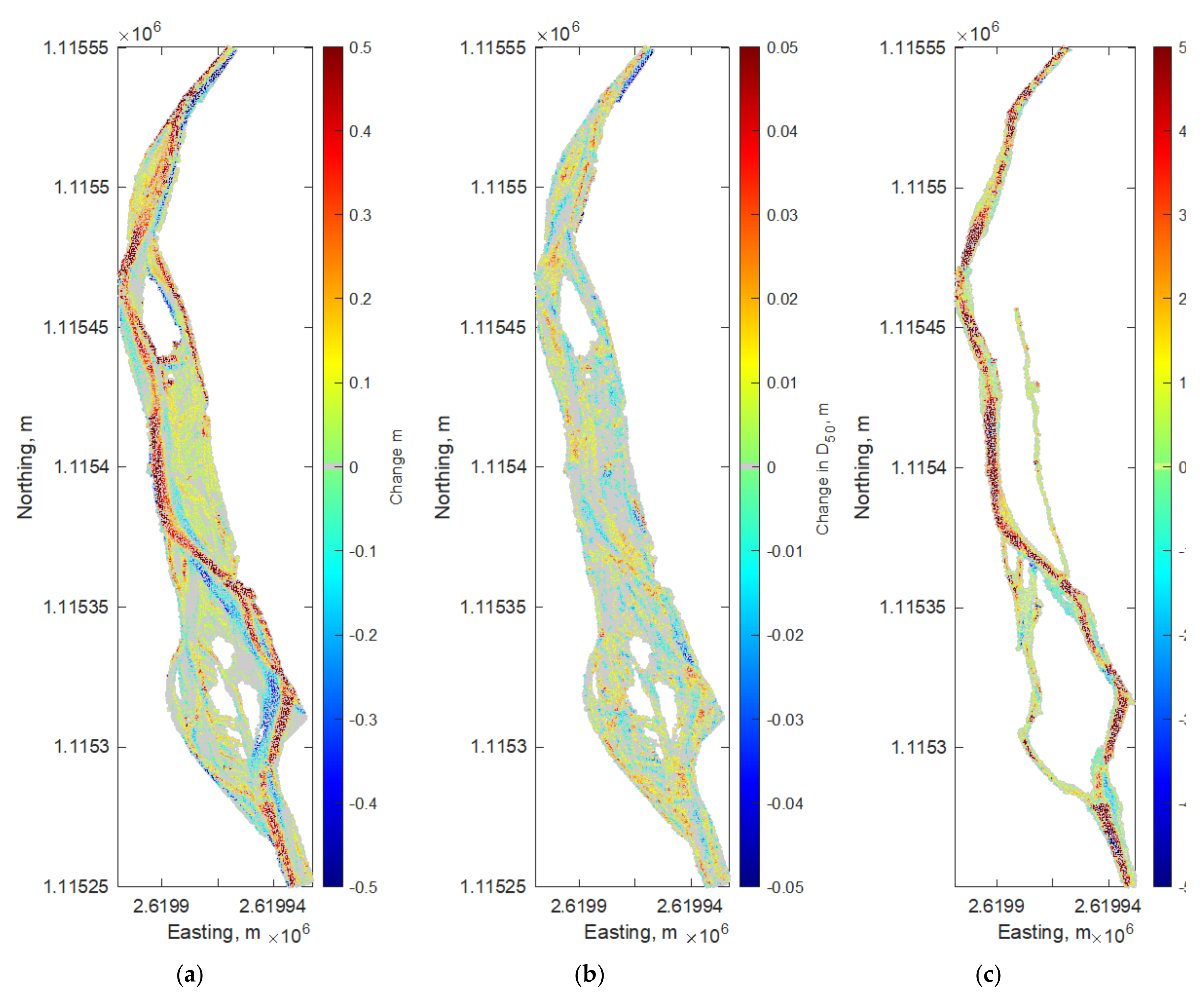
5. Channel Change, Sedimentological Change, and Habitat during the MFF: UAV-Derived Data

These three broad issues imply the need for results from the geospatial and modeling analyses shown in Figure 1, which were enabled by the acquisition of UAV-based photogrammetric data.

5.1. Results

Differencing of DEMs resulted in an estimate of the net change between the two surveys: a fill of 0.077 ± 0.022 m. This change was not spatially uniform (Figure 6a) but concentrated largely in the low-flow channel. In the upstream half of the reach, the low-flow channel migrated toward the true left, and there was generally fill of secondary branches. In the downstream half of the reach, there was general deposition, again focused on the low-flow channel. The texture-based image analysis showed that the median grain size in the reach was generally coarser after the flood (Figure 7); quantitatively, the reach-scale mean of the median grain size increased from 0.0139 ± 0.0078 m to 0.0161 ± 0.0096 m, statistically significant at p < 0.001. The changes in grain size were not homogeneous but spatially organized (Figure 6b). Qualitative comparison of Figure 6a,b suggests grain-size fining in zones of erosion and grain-size coarsening in zones of deposition, and this appears also to be the case quantitatively (Figure 8), with sites with coarsening more likely to be depositional than erosional. However, it is less clear that sites associated with fining are more likely to be erosional than depositional. Indeed, inspection of the imagery showed some deposition of fine sediment in zones of both deposition and erosion.

There was some relationship between erosion and deposition patterns and grain size (Figure 6c). Data were limited to the low-flow channel as it was assumed that this is where fine sediment deposition was most likely to occur at low flows and colmation was most likely to develop as the associated biological and biochemical processes require continued access to water. There were clear zones of blue where the depth of erosion was many multiples of the initial grain size. However, the much clearer signal constituted the zones of red where the thickness of deposition was many multiples of grain size. This confirms that a major consequence of the flushing event was the fill of the main low-flow channel by coarser sediment than that present at the start of the event.

We calculated the uplift in ${\theta }_c$ needed to prevent sediment transport at the base flow (Figure 9a) and the extent to which the highest discharge during the flushing event exceeded the uplifted critical Shields stress (Figure 9b). There is a localized need for uplift in the main baseflow channel but not the secondary channels that were inundated at baseflow (Figure 9a). Evidence suggests that the uplift is biased toward zones with a D₅₀ in the sand or finer category with 44.4% of sand and finer locations requiring uplift, as compared with 9.9% of coarse gravel and coarser locations. This may be due to the presence of some colmation in the sand sites. The peak flow during the flushing event resulted in extensive zones where the modeled shear stress was greater than the modified (uplifted) critical shear stress (Figure 9b). Only 2.2% of sites had a shear stress less than the critical value, and 87.5% of sites had a shear stress more than three times the critical value. Thus, the peak flow was likely to be capable of substantially eroding the low-flow channel. However, the low-flow channel was largely filled by sediment during the event, with the erosion being related more to channel migration (Figure 6a).

Small increases in discharge can result in a spatially extensive capacity for the transport of sand material and finer (Figure 10a), exceeding 90% of the surface of the low-flow channel for a discharge of 1 m³·s⁻¹. Indeed, as discharge increased, there was a rapid rise in the spatial extent of potential sand transport (Figure 10b). This remained high throughout both MFFa and MFFb and the clearwater flows CWa and CWb.

In qualitative terms, the total habitat availability (Figure 11a) reflects the relative numbers of insects present (Baetidae > Perlodidae > Limnephilidae > Chironomidae) (Table 2). The total habitat availability increased progressively with discharge, rapidly to about 0.25 m³·s⁻¹, more slowly to about 1.0 m³·s⁻¹ and, then, with some variability between families, more rapidly again. These changes reflect the fact that, at 0.25 m³·s⁻¹, the wetted perimeter of the low-flow channel was at its maximum and, thereafter, increases in flow were delivered by increases in depth and velocity. Total habitat did not then increase as rapidly until the onset of inundation of new zones at discharges greater than 1m³·s⁻¹. The weighted habitat decreased with discharge (Figure 11b), i.e., the rate of new habitat gain was slower than the rate of increase of the inundated area. This occurred a little later for Baetidae, reflecting its suitability to higher bed shear stresses than other families.

The total and weighted habitat availabilities were simulated through time (Figure 11c,d) under the assumption that the substrates remained constant through the flood and that shear stresses were only driven by changes in discharge and not morphological change or substrate change. Although these plots should be taken with caution as a result of these assumptions, they show how. as discharge increased during the start of the flushing event, the absolute habitat available increased but the weighted habitat availability decreased. Understanding this asymmetric response needs to also consider where the habitat became suitable as the discharge rises (or falls). As discharge increased, the optimal habitat (Figure 11e, shown here only for Baetidae) initially moved to the margins of the primary channel occupied at 0.25 m³·s⁻¹. A more marked change occurred at around 3 m³·s⁻¹ when bar tops became progressively inundated. Although not all bar tops were inundated at the highest discharge (Figure 11e), the margins of the active floodplain had the optimal habitat at these extreme flows.

5.2. Discussion

Figure 5 suggested that the MFF resulted in a net loss (900 tons, Figure 5b) of fine sediment from the study reach. Expressing this as a volume loss per unit area, and using the maximum flood extent as modeled, this was equivalent to a loss of 0.043 ± 0.0015 m of fine sediment per m². The photogrammetric analysis (Figure 6a) suggested a net deposition of 0.077 ± 0.022 m. The only situation that can reconcile these estimates is the net deposition of coarser sediment in the reach and surface coarsening. This was confirmed in the changes in the patterns of grain-size change before and after the entire flow trial (Figure 6b; Figure 7). Coarse sediment deposition requires sediment supply from upstream. Thus, the MFF was able to clean gravel (the net fine sediment loss) but also to supply coarse sediment. This is perhaps surprising given that the study reach is downstream from a dam that disconnects coarse sediment supply and that the flushing flows themselves only supplied fine sediment from behind the dam. However, it may reflect the fact that there are ungauged tributaries between the dam and the study reach (Figure 2a), which aerial imagery suggests are active in the supply of sediment. This observation cautions against generic recommendations for these kinds of flushing flows and emphasizes the need to consider the local catchment setting.

Equally surprising was the extent of channel reworking (Figure 6a) to many multiples of grain size (Figure 6c) given that the peak discharge during the MFF was still substantially lower (60%) than what was initially thought necessary for this stream were it to have a dedicated artificial flood rather than modification of the flushing flow. Thus, the MFF delivered a key goal for management of this stream—substantial working of the stream bed. Indeed, the fact that there was net coarsening (Figure 7) suggests that the MFF achieved a good compromise between sufficient gravel transport to release fine sediment from the bed (Figure 5) but not so much that there was substantial gravel loss [82] given the observed coarsening (Figure 7). The fact that there was much less loss of fine sediment during MFFb (Figure 5) suggested that much of the bed coarsening suggested in Figure 7 was likely to have been during the first flush, MFFa.

By coupling the remotely sensed bathymetric and grain-size data with the hydrodynamic modeling, it was possible to define more precisely the discharge necessary to flush the stream bed, as well as to prevent fine sediment deposition. The uplift in the critical Shields stress was greater than is typically reported (e.g., [111]) but also spatially variable over quite small distances (Figure 9a). The uplift is likely to reflect two different processes: (1) in zones of coarser sediment, a tendency toward the hiding of finer grains by coarser grains, and (2) in zones of fine sediment, the development of cohesion due to possible stream colmation. Indeed, the effects of colmation on the critical Shields stress are poorly known [19]. The inverse approach used here allowed for a more realistic parameterization of the critical Shields stress for estimating the onset of transport.

The ease of sand transport in the low flow (Figure 10), as well as the rapid flushing of fine sediment in the monitoring data (Figure 5a), reflects field observations that the bed was only poorly colmated and that the uplift was most likely due to hiding effects. If the objective of the flushing flows is to simply remove fine sediment, rather than to also rework the bed, smaller flushing flows than the two used here are likely to be sufficient. A similar conclusion can be made with respect to the rinsing flows; the discharge required to prevent fine sediment deposition in the stream bed is relatively low, lower than either of the two clear water discharges tested here (Figure 10b). The study reach here is about 13 km upstream from the junction with the Rhone River and, to be sure that fine sediment flushed from the reach is completely evacuated from the tributary, it is probable that a longer-duration but lower-magnitude clear-water flow will be of more value that the shorter-duration but higher-magnitude clear-water flows tried here. Indeed, for this system, relatively low-magnitude clear-water releases (no greater than 1m³·s⁻¹) may be all that is needed.

Bringing in habitat considerations further supports this conclusion (Figure 11). The relationship between changes in habitat quantity (Figure 11a) and quality (Figure 11b) and discharge is nonlinear and reflects a strong morphological control as reported for a similar site [25]. This observation has important implications for the magnitude of the minimum flows that should be released downstream from dams as, once the low-flow channel was wetted, total habitat increased at a slower rate than habitat quality decreases. The spatially distributed analysis (e.g., Figure 11e) emphasized that habitat increased as discharge rises were spatially distributed. Up until a certain discharge magnitude, the optimal discharge shifted only marginally in space (Figure 11a), increasing the probability that an insect is able to find a local refuge as flow increases, such as due to enforced drift [84,137,138]. Keeping the flushing flow to a maximum of around 3 m³·s⁻¹ is not only likely to remove unwanted accumulations of fine sediment but is also less likely to result in negative impacts on stream biota (Figure 11e).

6. The Role of UAV SfM-MVS Photogrammetry in Setting Environmental Flows

The previous section showed how the methodology described in Figure 1 allowed a much richer understanding of how to set environmental flows in this stream. The methodology has two distinct advantages. On the one hand, it allows proposals for setting environmental flows to be evaluated in pilot projects by quantifying the patterns of erosion and deposition and grain-size change. On the other hand, the hydraulic and habitat modeling shows how it can be used to inform the design of potential future environmental flows, whether minimum flows or flushing flows. Notably, following from evidence in Figure 10 and Figure 11, it was possible to suggest that both the peak flows and the clearwater rinsing flows in the MFF were higher than necessary. In turn, these underpinned an improved parameterization of the sediment transport process, in terms of distributed patterns of grain size (Figure 4) and the uplift in the critical Shields stress needed to represent hiding effects and possibly colmation (Figure 10), as well as the ability to obtain distributed information on the patterns of bed shears stress and to use these in habitat models to understand changes in the spatial organization of habitat as discharge changes.

This provides a methodological framework for optimizing the operation of dams such that we can both maintain the quantity of non-fossil-fuel energy production whilst also minimizing negative environmental impacts. It is the remote sensing that we present that allows the spatially explicit analyses, which in turn allow trials to be monitored and proposals to be designed. However, the value of UAV-based SfM-MVS surveys is not restricted to the evaluation of flushing flows. This paper showed for the first time that high-resolution SfM-MVS orthoimagery can be used to quantify grain-size changes (and not just grain size at any one time) and, hence, quantify the relationships between grain size change erosion and deposition in streams. Not only should spatially distributed grain-size data allow for better application of models of river channel change, the ability to relate grain-size data to erosion and deposition should improve the formulation of such models (such as in relation to colmation, as illustrated here). The same applies to habitat modeling. The need for this to be spatially distributed has been noted as critical for some time [27,28,29]; however, as illustrated with the initial development of the habitat model described here [129], the challenge remains to acquire the stream bathymetry for such applications [30]. It is only really with the development of UAV-based SfM-MVS photogrammetry that this habitat modeling approach has become feasible.

That said, this study also emphasizes the complementarity of traditional monitoring to UAV-based methodologies such as that proposed in Figure 1. The data provided from UAV surveys are spatially rich (e.g., Figure 6) but temporally poor, here only providing a before and after perspective. The high levels of turbidity associated with the flushing event (Figure 5) preclude the measurement of stream bathymetry through repeating flights during the event as the optical depth tends to zero throughout the study area. The suspended sediment monitoring, however, provides temporally rich data but nothing on the spatial patterns that lead to the measured sediment signals. In this sense, the data from UAV surveys is most powerful when it is combined with other kinds of environmental monitoring. Here, by coupling the UAV surveys with the suspended sediment monitoring, it was possible to show that the net surface coarsening (Figure 6b and Figure 7) is likely to have been partially realized early on in the experiment through the evacuation of suspended sediment (Figure 5). The UAV survey itself also needed hydrodynamic modeling to obtain the physical parameters that drive sediment transport (here, the bed shear stress and the grain-size data needed for the critical shear stress). Similarly, the habitat analyses and mapping (Figure 11), which allow an environmental flow to be optimized against other goals (e.g., removing colmation), were also underpinned by the hydrodynamic modeling. The key point is that the value of UAV-based SfM-MVS photogrammetry is only realized through combining its outputs with other monitoring and modeling methods. That said, the next development needed in this methodology would involve dynamic within-event coupled modeling of flow hydraulics, sediment transport, and channel change. Such models do exist, and they are effective at reproducing general river morphodynamics (e.g., [139]) but often struggle to provide the detail [140] needed to inform the design of environmental flows.

Although this study focused on only a 300 m reach of a 15 km long stream (i.e., ca. 5% of the stream length), this was justified by careful choice and justification of the reach. In theory, there is no limit to how short the reach has to be; in practice, a longer reach necessitates a longer data acquisition time, as well as a greater probability of additional survey problems such as bankside trees or bridges that reduce the ease of application of a UAV-based method. Many of these practical issues were less relevant in this study because of a focus on the reach of an Alpine stream at an altitude close to the tree line. The field survey work required in this study was only 2 days.

The last 30 years has seen a revolution in our ability to measure stream bathymetry rapidly and easily, notably in the analytical methods needed to deal with the challenges posed by inundation [33,34,36,94] and in determining grain size [47,48,49,50,55]. However, operationalizing Figure 1 remains dependent upon one critical stage: effective handling of UAV-derived imagery. The initial excitement of the potential of UAV-based SfM-MVS photogrammetry [87] has resulted in a more measured realization that many of the traditional controls for the success of a photogrammetric project remain, notably the calibration of internal camera geometry. This can lead to important systematic errors in derived digital elevation data that significantly impact the ability to identify morphological change (e.g., Figure 6a). Long-established lessons regarding how to calibrate nonmetric cameras in analog and analytical photogrammetry (e.g., [141,142]) still apply. A number of studies have sought to provide guidance on how to optimize SfM-MVS image data collection and processing (e.g., [143,144,145,146]); however, it is only recently that there has been the controlled investigation of what determines the internal geometry of cameras used in a UAV-based SfM-MVS photogrammetric framework (e.g., [101,147]). There is growing evidence that such guidance cannot be generalized either between UAV systems or between environments using the same UAV system [101]. Thus, there remains a considerable technical challenge in making sure that the UAV-based SfM-MVS photogrammetry is undertaken correctly if it is to be used as an environmental flow methodology. Given these uncertainties, it is also important to make recourse to basic guidelines on the correct use of SfM-MVS photogrammetry [104] and to include assessment of the quality of the derived data (e.g., confirming that there are no significant elevation and grain-size changes estimated in zones that were not inundated during the modified flushing flow).

7. Conclusions

This paper proposed a methodology based upon UAV-SfM photogrammetry that can be used to set environmental flows (Figure 1) and illustrated this methodology for the case of a modification to a flushing flow for an Alpine stream. Integral to this methodology is the use of UAV-based SfM-MVS photogrammetry as a means of driving a suite of existing hydrodynamic, morphodynamic, and habitat analyses. The methodology can be the basis of not only testing proposed environmental flows, but also designing options for future environmental flows. The most novel and valuable part of the method is the ability to incorporate distributed data on grain size, derived from orthorectified UAV-based imagery, which drives both sediment transport and habitat availability in the kinds of stream studied here. In this application, the methodology informed assessment of the extent to which a trial-modified flushing flow resulted in coarsening of sediment in the active zone of the study reach. It was used to parameterize an analysis of likely sediment entrainment in terms of inclusion of spatially distributed information on both the critical grain size and the uplift in the critical Shields stress needed due to packing and colmation effects. It was also used as part of a spatially explicit habitat analysis. However, we also argue that the real value of the derived spatially rich data is only realized when it is combined with more traditional monitoring methods that are more temporally rich.

The case used here to illustrate the methodology showed that the pilot-modified flushing flow resulted in significant reworking of the stream bed, in terms of both channel change and net removal of fine sediment. Initial proposals for the environmental flow in this basin proposed a much larger, clear-water flood, which posed technical and security challenges. The MFF here was based upon the annual flushing of an upstream dam, modified to include a clear water or rinsing flow after the flushing of the dam. The combined analyses (1) suggested that the flood peaks were larger than were needed, (2) indicated that only a single flood peak was necessary, despite the flushing of the dam potentially delivering large amounts of fine sediment, (3) showed that the sediment coarsening was likely also to be impacted by supply from nonregulated tributaries, often overlooked in this kind of study, and (4) allowed us to conclude that a lower-magnitude but longer-duration rinsing flow after the flushing flow would be valuable for the system.

References

1. Parasiewicz, P.; Schmutz, S.; Moog, O. The effect of managed hydropower peaking on the physical habitat, benthos and fish fauna in the River Bregenzerach in Austria. Fish. Manag. Ecol. 1998, 5, 403–417. [Google Scholar] [CrossRef]
2. Bunn, S.E.; Arthington, A.H. Basic Principles and Ecological Consequences of Altered Flow Regimes for Aquatic Biodiversity. Environ. Manag. 2002, 30, 492–507. [Google Scholar] [CrossRef] [PubMed] [Green Version]
3. Poff, N.L.; Zimmerman, J.K.H. Ecological responses to altered flow regimes: A literature review to inform the science and management of environmental flows. Freshw. Biol. 2010, 55, 194–205. [Google Scholar] [CrossRef]
4. Poff, N.L.; Allan, J.D.; Bain, M.B.; Karr, J.R.; Prestegaard, K.L.; Richter, B.D.; Sparks, R.E.; Stromberg, J.C. The Natural Flow Regime. Bioscience 1997, 47, 769–784. [Google Scholar] [CrossRef]
5. The Brisbane Declaration. Environmental Flows are Essential for Freshwater Ecosystem Health and Human Well-Being. In Proceedings of the 10th International River Symposium and International Environmental Flows Conference, Brisbane, Australia, 3–6 September 2007.
6. Dyson, M.; Bergkamp, G.; Scanlon, J. Flow: The Essentials of Environmental Flows; IUCN: Gland, Switzerland; Cambridge, UK, 2003. [Google Scholar]
7. Petts, G.E. Instream Flow Science For Sustainable River Management. JAWRA J. Am. Water Resour. Assoc. 2009, 45, 1071–1086. [Google Scholar] [CrossRef] [Green Version]
8. Arthington, A.H. Environmental Flows: Saving Rivers in the Third Millennium; University of California Press: Berkeley, CA, USA, 2012. [Google Scholar]
9. Whipple, A.A.; Viers, J. Coupling landscapes and river flows to restore highly modified rivers. Water Resour. Res. 2019, 55, 4512. [Google Scholar] [CrossRef]
10. Ashworth, P.J.; Ferguson, R.I. Interrelationships of channel processes, changes and sediments in a proglacial braided river, Geografiska Annaler: Series A. Phys. Geogr. 1986, 68, 361–371. [Google Scholar]
11. Lancaster, J.; Hildrew, A.G. Flow Refugia and the Microdistribution of Lotic Macroinvertebrates. J. N. Am. Benthol. Soc. 1993, 12, 385–393. [Google Scholar] [CrossRef]
12. Möbes-Hansen, B.; Waringer, J.A. The Influence of Hydraulic Stress on Microdistribution Patterns of Zoobenthos in a Sandstone Brook (Weidlingbach, Lower Austria). Int. Rev. Hydrobiol. 1998, 83, 381–396. [Google Scholar] [CrossRef]
13. Armstrong, J.; Kemp, P.; Kennedy, G.; Ladle, M.; Milner, N. Habitat requirements of Atlantic salmon and brown trout in rivers and streams. Fish. Res. 2003, 62, 143–170. [Google Scholar] [CrossRef]
14. Merigoux, S.; Doledec, S. Hydraulic requirements of stream communities: A case study on invertebrates. Freshw. Biol. 2004, 49, 600–613. [Google Scholar] [CrossRef]
15. Dolédec, S.; Lamouroux, N.; Fuchs, U.; Mérigoux, S. Modelling the hydraulic preferences of benthic macroinvertebrates in small European streams. Freshw. Biol. 2007, 52, 145–164. [Google Scholar] [CrossRef]
16. Mérigoux, S.; Lamouroux, N.; Olivier, J.-M.; Dolédec, S. Invertebrate hydraulic preferences and predicted impacts of changes in discharge in a large river. Freshw. Biol. 2009, 54, 1343–1356. [Google Scholar] [CrossRef]
17. Wood, P.J.; Toone, J.; Greenwood, M.T.; Armitage, P.D. The response of four lotic macroinvertebrate taxa to burial by sediments. Archiv. für Hydrobiol. 2005, 163, 145–162. [Google Scholar] [CrossRef]
18. Conroy, E.; Turner, J.N.; Rymszewicz, A.; Bruen, M.; O’Sullivan, J.J.; Lawler, D.M.; Stafford, S.; Kelly-Quinn, M. Further insights into the responses of macroinvertebrate species to burial by sediment. Hydrobiologia 2017, 805, 399–411. [Google Scholar] [CrossRef]
19. Wharton, G.; Mohajeri, S.H.; Righetti, M. The pernicious problem of streambed colmation: A multi-disciplinary reflection on the mechanisms, causes, impacts, and management challenges. WIREs Water 2017, 4, e1231. [Google Scholar] [CrossRef]
20. Orr, C.H.; Kroiss, S.J.; Rogers, K.L.; Stanley, E.H. Downstream benthic responses to small dam removal in a coldwater stream. River Res. Appl. 2008, 24, 804–822. [Google Scholar] [CrossRef]
21. Müller, M.P.; McKnight, D.M.; Cullis, J.D.; Greene, A.; Vietti, K.; Liptzin, D. Factors controlling streambed coverage of Didymosphenia germinate in two regulated streams in the Colorado front range. Hydrobiologia 2009, 630, 207–218. [Google Scholar] [CrossRef] [Green Version]
22. Fuller, R.L.; Doyle, S.; Levy, L.; Owens, J.; Shope, E.; Vo, L.; Wolyniak, E.; Small, M.J.; Doyle, M.W. Impact of regulated releases on periphyton and macroinvertebrate communities: The dynamic relationship between hydrology and geomorphology in frequently flooded rivers. River Res. Appl. 2010, 27, 630–645. [Google Scholar] [CrossRef]
23. Cullis, J.D.S.; Stanish, L.F.; McKnight, D.M. Diel flow pulses drive particulate organic matter transport from microbial mats in a glacial meltwater stream in the McMurdo Dry Valleys. Water Resour. Res. 2014, 50, 86–97. [Google Scholar] [CrossRef]
24. Wohl, E.; Bledsoe, B.P.; Jacobson, R.B.; Poff, N.L.; Rathburn, S.L.; Walters, D.M.; Wilcox, A.C. The Natural Sediment Regime in Rivers: Broadening the Foundation for Ecosystem Management. Bioscience 2015, 65, 358–371. [Google Scholar] [CrossRef] [Green Version]
25. Gabbud, C.; Bakker, M.; Clemençon, M.; Lane, S.N. Causes of the severe loss of macrozoobenthos in Alpine streams subject to repeat hydropower flushing events. Water Resour. Res. 2019, 55, 10056–10081. [Google Scholar] [CrossRef]
26. Bovee, K.; Millhous, R. Hydraulic Simulation in Instream Flow Studies: Theory and Techniques; FWS/OBS-78/33; US Fish and Wildlife Service: Washington, DC, USA, 1978. [Google Scholar]
27. Ghanem, A.; Steffler, P.; Hicks, F.; Katopodis, C. Two-dimensional finite element flow modeling of physical fish habitat. In Proceedings of the 1st International Association for Hydraulic Research Symposium on Habitat Hydraulics, Trondheim, Norway, 18–20 August 1994; Norwegian Institute of Technology: Trondheim, Norway, 1994; pp. 84–89. [Google Scholar]
28. Leclerc, M.; Boudreault, A.; Bechara, T.A.; Corfa, G. Two-Dimensional Hydrodynamic Modeling: A Neglected Tool in the Instream Flow Incremental Methodology. Trans. Am. Fish. Soc. 1995, 124, 645–662. [Google Scholar] [CrossRef]
29. Hardy, T.B. The future of habitat modeling and instream flow assessment techniques. Regul. Riv. Res. Manag. 1998, 14, 405–420. [Google Scholar] [CrossRef]
30. Benjankar, R.; Tonina, D.; McKean, J.A. One-dimensional and two-dimensional hydrodynamic modeling derived flow properties: Impacts on aquatic habitat quality predictions. Earth Surf. Process. Landf. 2014, 40, 340–356. [Google Scholar] [CrossRef]
31. Leclerc, M. Ecohydraulics: A new interdisciplinary frontier for CFD. In Computational Fluid Dynamics: Applications in Environmental Hydraulics; Bates, P.D., Lane, S.N., Ferguson, R.I., Eds.; Wiley: Chichester, UK, 2005; pp. 429–459. [Google Scholar]
32. Lane, S.N.; Chandler, J.H.; Richards, K.S. Developments in monitoring and terrain modelling small-scale river-bed topography. Earth Surface Process Landf. 1994, 19, 349–368. [Google Scholar] [CrossRef]
33. Westaway, R.M.; Lane, S.N.; Hicks, D.M. The development of an automated correction procedure for digital photogrammetry for the study of wide, shallow, gravel-bed rivers. Earth Surface Process Landf. 2000, 25, 209–226. [Google Scholar] [CrossRef]
34. Westaway, R.M.; Lane, S.N.; Hicks, D.M. Remote sensing of clearwater, shallow, gravel-bed rivers using digital photogrammetry. Photogramm. Eng. Remote Sens. 2001, 67, 1271–1282. [Google Scholar]
35. Westaway, R.M.; Stutenbecker, L.; Hicks, D.M. Remote survey of large-scale braided, gravel-bed rivers using digital photogrammetry and image analysis. Int. J. Remote Sens. 2003, 24, 795–815. [Google Scholar] [CrossRef]
36. Lane, S.N.; Widdison, P.E.; Thomas, R.E.; Ashworth, P.J.; Best, J.; Lunt, I.A.; Smith, G.H.S.; Simpson, C.J. Quantification of braided river channel change using archival digital image analysis. Earth Surf. Process. Landf. 2010, 35, 971–985. [Google Scholar] [CrossRef]
37. Kinzel, P.J.; Legleiter, C.J.; Nelson, J.M. Mapping River Bathymetry With a Small Footprint Green LiDAR: Applications and Challenges1. JAWRA J. Am. Water Resour. Assoc. 2012, 49, 183–204. [Google Scholar] [CrossRef]
38. Mandlburger, G.; Hauer, C.; Wieser, M.; Pfeifer, N. Topo-bathymetric LiDAR for monitoring river morphodynamics and instream Hhbitats—A case study at the Pielach River. Remote Sens. 2015, 7, 6160–6195. [Google Scholar] [CrossRef] [Green Version]
39. McKean, J.A.; Tonina, D.; Bohn, C.; Wright, C. Effects of bathymetric lidar errors on flow properties predicted with a multi-dimensional hydraulic model. J. Geophys. Res. Earth Surf. 2014, 119, 644–664. [Google Scholar] [CrossRef]
40. Tonina, D.; Mckean, J.A.; Benjankar, R.M.; Wright, C.W.; Goode, J.R.; Chen, Q.; Reeder, W.J.; Carmichael, R.A.; Edmondson, M.R. Mapping river bathymetries: Evaluating topobathymetric LiDAR survey. Earth Surf. Process. Landf. 2019, 44, 507–520. [Google Scholar] [CrossRef]
41. Tonina, D.; Mckean, J.A.; Benjankar, R.M.; Yager, E.; Carmichael, R.A.; Chen, Q.; Carpenter, A.; Kelsey, L.G.; Edmondson, M.R. Evaluating the performance of topobathymetric LiDAR to support multi-dimensional flow modelling in a gravel-bed mountain stream. Earth Surf. Process. Landforms 2020. [Google Scholar] [CrossRef]
42. Lane, S.N. Acting, predicting and intervening in a socio-hydrological world. Hydrol. Earth Syst. Sci. 2014, 18, 927–952. [Google Scholar] [CrossRef] [Green Version]
43. Gardner, J.T.; Ashmore, P. Geometry and grain-size characteristics of the basal surface of a braided river deposit. Geology 2011, 39, 247–250. [Google Scholar] [CrossRef]
44. Leduc, P.; Ashmore, P.; Gardner, J.T. Grain sorting in the morphological active layer of a braided river physical model. Earth Surface Dyn. 2015, 3, 577–585. [Google Scholar]
45. Reid, H.; Williams, R.D.; Brierley, G.; Coleman, S.; Lamb, R.; Rennie, C.D.; Tancock, M. Geomorphological effectiveness of floods to rework gravel bars: Insight from hyperscale topography and hydraulic modelling. Earth Surf. Process. Landforms 2018, 44, 595–613. [Google Scholar] [CrossRef]
46. Newson, M.D.; Newson, C.L. Geomorphology, ecology and river channel habitat: Mesoscale approaches to basin-scale challenges. Prog. Phys. Geogr. Earth Environ. 2000, 24, 195–217. [Google Scholar] [CrossRef]
47. Carbonneau, P.E.; Bergeron, N.E.; Lane, S.N. Texture based image segmentation applied to the quantification of superficial sand in salmonid river gravels. Earth Surface Process. Landf. 2005, 30, 121–127. [Google Scholar] [CrossRef]
48. Carbonneau, P.E.; Lane, S.N.; Bergeron, N.E. Catchment-scale mapping of surface grain size in gravel bed rivers using airborne digital imagery. Water Resour. Res. 2004, 40. [Google Scholar] [CrossRef] [Green Version]
49. Carbonnneau, P.; Bizzi, S.; Marchetti, G. Robotic photosieving from low-cost multirotor sUAS: A proof-of-concept. Earth Surf. Process. Landf. 2018, 43, 1160–1166. [Google Scholar] [CrossRef] [Green Version]
50. Buscombe, D.; Rubin, D.M.; Warrick, J.A. A universal approximation of grain size from images of noncohesive sediment. J. Geophys. Res. Space Phys. 2010, 115. [Google Scholar] [CrossRef] [Green Version]
51. Dugdale, S.J.; Carbonneau, P.E.; Campbell, D. Aerial photosieving of exposed gravel bars for the rapid calibration of airborne grain size maps. Earth Surf. Process. Landf. 2010, 35, 627–639. [Google Scholar] [CrossRef]
52. Black, M.; Carbonneau, P.; Church, M.; Warburton, J. Mapping sub-pixel fluvial grain sizes with hyperspatial imagery. Sedimentology 2013, 61, 691–711. [Google Scholar] [CrossRef] [Green Version]
53. Woodget, A.S.; Austrums, R. Subaerial gravel size measurement using topographic data derived from a UAV-SfM approach. Earth Surf. Process. Landf. 2017, 42, 1434–1443. [Google Scholar] [CrossRef]
54. Woodget, A.S.; Fyffe, C.L.; Carbonneau, P.E. From manned to unmanned aircraft: Adapting airborne particle size mapping methodologies to the characteristics of sUAS and SfM. Earth Surf. Process. Landf. 2018, 43, 857–870. [Google Scholar] [CrossRef]
55. Buscombe, D. SediNet: A configurable deep learning model for mixed qualitative and quantitative optical granulometry. Earth Surf. Process. Landf. 2020, 45, 638–651. [Google Scholar] [CrossRef]
56. Gabbud, C.; Lane, S.N. Ecosystem impacts of Alpine water intakes for hydropower: The challenge of sediment management. Wiley Interdiscip. Rev. Water 2015, 3, 41–61. [Google Scholar] [CrossRef]
57. Bakker, M.; Costa, A.; Silva, T.A.; Stutenbecker, L.; Girardclos, S.; Loizeau, J.-L.; Molnar, P.; Schlunegger, F.; Lane, S.N. Combined Flow Abstraction and Climate Change Impacts on an Aggrading Alpine River. Water Resour. Res. 2018, 54, 223–242. [Google Scholar] [CrossRef]
58. Brooker, M.P.; Hemsworth, R.J. The effect of the release of an artificial discharge of water on invertebrate drift in the R. Wye, Wales. Hydrobiology 1978, 59, 155–163. [Google Scholar] [CrossRef]
59. Cushman, R.M. Review of Ecological Effects of Rapidly Varying Flows Downstream from Hydroelectric Facilities. N. Am. J. Fish. Manag. 1985, 5, 330–339. [Google Scholar] [CrossRef]
60. Moog, O. Quantification of daily peak hydropower effects on aquatic fauna and management to minimize environmental impacts. Regul. Rivers Res. Manag. 1993, 8, 5–14. [Google Scholar] [CrossRef]
61. Lauters, F.; Lavandier, P.; Lim, P.; Sabaton, C.; Belaud, A. Influence of hydropeaking on invertebrates and their relationship with fish feeding habits in a Pyrenean river. Regul. Riv. Res. Manag. 1996, 12, 563–573. [Google Scholar] [CrossRef]
62. Cereghino, R.; Lavandier, P. Influence of hypolimnetic hydropeaking on the distribution and population dynamics of Ephemeroptera in a mountain stream. Freshw. Biol. 1998, 40, 385–399. [Google Scholar] [CrossRef] [Green Version]
63. Smokorowski, K.E.; Metcalfe, R.A.; Finucan, S.D.; Jones, N.; Marty, J.; Power, M.; Pyrce, R.S.; Steele, R. Ecosystem level assessment of environmentally based flow restrictions for maintaining ecosystem integrity: A comparison of a modified peaking versus unaltered river. Ecohydrology 2010, 4, 791–806. [Google Scholar] [CrossRef]
64. Schmutz, S.; Bakken, T.H.; Friedrich, T.; Greimel, F.; Harby, A.; Jungwirth, M.; Melcher, A.; Unfer, G.; Zeiringer, B. Response of Fish Communities to Hydrological and Morphological Alterations in Hydropeaking Rivers of Austria. River Res. Appl. 2014, 31, 919–930. [Google Scholar] [CrossRef] [Green Version]
65. Schülting, L.; Feld, C.K.; Graf, W. Effects of hydro- and thermopeaking on benthic macroinvertebrate drift. Sci. Total Environ. 2016, 573, 1472–1480. [Google Scholar] [CrossRef]
66. Schülting, L.; Feld, C.K.; Zeiringer, B.; Huđek, H.; Graf, W. Macroinvertebrate drift response to hydropeaking: An experimental approach to assess the effect of varying ramping velocities. Ecohydrology 2018, 12, e2032. [Google Scholar] [CrossRef]
67. Gabbud, C.; Robinson, C.T.; Lane, S.N. Summer is in winter: Disturbance-driven shifts in macroinvertebrate communities following hydroelectric power exploitation. Sci. Total Environ. 2019, 650, 2164–2180. [Google Scholar] [CrossRef] [PubMed] [Green Version]
68. Willis, C.M.; Griggs, G.B. Reductions in Fluvial Sediment Discharge by Coastal Dams in California and Implications for Beach Sustainability. J. Geol. 2003, 111, 167–182. [Google Scholar] [CrossRef]
69. Meissner, T.; Schutt, M.; Sures, B.; Feld, C.K. Riverine regime shifts through reservoir dams reveal options for ecological management. Ecol. App. 2018, 28, 1898–1908. [Google Scholar] [CrossRef] [PubMed]
70. Zhang, Y.; Hubbard, S.; Finsterle, S. Factors Governing Sustainable Groundwater Pumping near a River. Ground Water 2010, 49, 432–444. [Google Scholar] [CrossRef]
71. Gartner, J.; Renshaw, C.; Dade, W.; Magilligan, F.J. Time and depth scales of fine sediment delivery into gravel stream beds: Constraints from fallout radionuclides on fine sediment residence time and delivery. Geomorphology 2012, 151, 39–49. [Google Scholar] [CrossRef]
72. Andrews, E.D.; Pizzi, L.A. Origin of the Colorado River experimental flood in Grand Canyon. Hydrol. Sci. J. 2000, 45, 607–627. [Google Scholar] [CrossRef]
73. Jakob, C.; Robinson, C.T.; Uehlinger, U. Longitudinal effects of experimental floods on stream benthos downstream from a large dam. Aquat. Sci. 2003, 65, 223–231. [Google Scholar] [CrossRef] [Green Version]
74. Robinson, C.T.; Uehlinger, U.; Monaghan, M.T. Effects of a multi-year experimental flood regime on macroinvertebrates downstream of a reservoir. Aquat. Sci. 2003, 65, 210–222. [Google Scholar] [CrossRef] [Green Version]
75. Mannes, S.; Robinson, C.T.; Uehlinger, U.; Scheurer, T.; Ortlepp, J.; Mürle, U.; Molinari, P. Ecological effects of a long-term flood program in a flow-regulated river. Rev. de Géographie Alpine 2008, 96, 125–134. [Google Scholar] [CrossRef] [Green Version]
76. Wright, S.A.; Kaplinski, M. Flow structures and sandbar dynamics in a canyon river during a controlled flood, Colorado River, Arizona. J. Geophys. Res. Space Phys. 2011, 116. [Google Scholar] [CrossRef] [Green Version]
77. Tonkin, J.D.; Death, R.G. The Combined Effects of flow regulation and an artificial flow release on a regulated river. River Res. Appl. 2014, 30, 329–337. [Google Scholar] [CrossRef]
78. Magdaleno, F. Experimental floods: A new era for Spanish and Mediterranean rivers? Environ. Sci. Policy 2017, 75, 10–18. [Google Scholar] [CrossRef]
79. Lessard, J.; Hicks, D.M.; Snelder, T.H.; Arscott, D.B.; Larned, S.T.; Booker, D.; Suren, A.M. Dam design can impede adaptive management of environmental flows: A case study from the Opuha Dam, New Zealand. Environ. Man. 2013, 51, 459–473. [Google Scholar] [CrossRef] [PubMed]
80. Battisacco, E.; Franca, M.J.; Schleiss, A.J. Sediment replenishment: Influence of the geometrical configuration on the morphological evolution of channel-bed. Water Resour. Res. 2016, 52, 8879–8894. [Google Scholar] [CrossRef]
81. Stähly, S.; Franca, M.J.; Robinson, C.T.; Schleiss, A.J. Sediment replenishment combined with an artificial flood improves river habitats downstream of a dam. Sci. Rep. 2019, 9, 1–8. [Google Scholar] [CrossRef]
82. Kondolf, G.M.; Wilcock, P.R. The Flushing Flow Problem: Defining and Evaluating Objectives. Water Resour. Res. 1996, 32, 2589–2599. [Google Scholar] [CrossRef]
83. Loire, R.; Grosprêtre, L.; Malavoi, J.-R.; Ortiz, O.; Piegay, H. What Discharge Is Required to Remove Silt and Sand Downstream from a Dam? An Adaptive Approach on the Selves River, France. Water 2019, 11, 392. [Google Scholar] [CrossRef] [Green Version]
84. Espa, P.; Brignoli, M.L.; Crosa, G.; Gentili, G.; Quadroni, S. Controlled sediment flushing at the Cancano Reservoir (Italian Alps): Management of the operation and downstream environmental impact. J. Environ. Manag. 2016, 182, 1–12. [Google Scholar] [CrossRef]
85. Grimardias, D.; Guillard, J.; Cattaneo, F. Drawdown flushing of a hydroelectric reservoir on the Rhô;ne River: Impacts on the fish community and implications for the sediment management. J. Environ. Manag. 2017, 197, 239–249. [Google Scholar] [CrossRef]
86. Doretto, A.; Bo, T.; Bona, F.; Apostolo, M.; Bonetto, D.; Fenoglio, S. Effectiveness of artificial floods for benthic community recovery after sediment flushing from a dam. Environ. Monit. Assess. 2019, 191, 88. [Google Scholar] [CrossRef]
87. Fonstad, M.A.; Dietrich, J.T.; Courville, B.C.; Jensen, J.L.; Carbonneau, P.E. Topographic structure from motion: A new development in photogrammetric measurement. Earth Surf. Process. Landf. 2013, 38, 421–430. [Google Scholar] [CrossRef] [Green Version]
88. Lane, S.N.; Richards, K.; Chandler, J.H. Developments in photogrammetry; the geomorphological potential. Prog. Phys. Geogr. Earth Environ. 1993, 17, 306–328. [Google Scholar] [CrossRef]
89. Lane, S.N.; Westaway, R.M.; Hicks, D.M. Estimation of erosion and deposition volumes in a large gravel-bed, braided river using synoptic remote sensing. Earth Surface Process. Landf. 2003, 28, 249–271. [Google Scholar] [CrossRef]
90. Snavely, N. Scene Reconstruction and Visualization from Internet Photo Collections. Ph.D. Thesis, University of Washington, Seattle, WA, USA, 2008. [Google Scholar]
91. Eltner, A.; Schneider, D. Analysis of Different Methods for 3D Reconstruction of Natural Surfaces from Parallel-Axes UAV Images. Photogramm. Rec. 2015, 30, 279–299. [Google Scholar] [CrossRef]
92. James, M.R.; Robson, S. Mitigating systematic error in topographic models derived from UAV and ground-based image networks. Earth Surf. Process. Landf. 2014, 39, 1413–1420. [Google Scholar] [CrossRef] [Green Version]
93. Butler, J.; Lane, S.N.; Chandler, J.H.; Porfiri, E. Through-Water Close Range Digital Photogrammetry in Flume and Field Environments. Photogramm. Rec. 2002, 17, 419–439. [Google Scholar] [CrossRef]
94. Dietrich, J.T. Bathymetric Structure-from-Motion: Extracting shallow stream bathymetry from multi-view stereo photogrammetry. Earth Surf. Process. Landf. 2017, 42, 355–364. [Google Scholar] [CrossRef]
95. Vetsch, D.; Siviglia, A.; Caponi, F.; Ehrbar, D.; Gerke, E.; Kammerer, S.; Koch, A.; Peter, S.; Vanzo, D.; Vonwiller, L.; et al. System Manuals of BASEMENT, Version 2.8. Laboratory of Hydraulics, Glaciology and Hydrology (VAW). ETH Zurich, 2018. Available online: http://www.basement.ethz.ch (accessed on 25 August 2020).
96. Tachet, H.; Bournaud, M.; Richoux, P.; Usseglio-Polatera, P. Invertébrés d’eau Douce—Systématique, Biologie, Écologie; CNRS Editions: Paris, France, 2010; 600p. [Google Scholar]
97. Wolman, M.G. A method of sampling coarse river-bed material. Trans. Am. Geophys. Union 1954, 35, 951–956. [Google Scholar] [CrossRef]
98. Shields, A. Application of Similarity Principles and Turbulence Research to Bed-Load Movement. Mitteilungen der Preußischen Versuchsanstalt für Wasserbau, 26; Preußische Versuchsanstalt für Wasserbau: Berlin, Germany, 1936. [Google Scholar]
99. Weingartner, R.; Aschwanden, H. Quantification des débits des cours d’eau des Alpes suisses et des influences anthropiques qui les affectent. Rev. de Géographie Alpine 1994, 82, 45–57. [Google Scholar] [CrossRef]
100. OFEFP. Débits Résiduels Convenables—Comment les Déterminer? Office Fédérale de l’environnement, des Forêts et du Paysage (OFEFP): Bern, Switzerland, 2000. [Google Scholar]
101. James, M.R.; Antoniazza, G.; Robson, S.; Lane, S.N. Mitigating systematic error in topographic models for geomorphic change detection: Moving beyond off-nadir imagery. Earth Surface Process. Landf. 2020, 45, 2251–2271. [Google Scholar] [CrossRef]
102. James, M.; Robson, S.C. Straightforward reconstruction of 3D surfaces and topography with a camera: Accuracy and geoscience application. J. Geophys. Res. Space Phys. 2012, 117, 03017. [Google Scholar] [CrossRef] [Green Version]
103. Smith, M.; Carrivick, J.; Quincey, D. Structure from motion photogrammetry in physical geography. Prog. Phys. Geogr. Earth Environ. 2016, 40, 247–275. [Google Scholar] [CrossRef]
104. James, M.R.; Chandler, J.H.; Eltner, A.; Fraser, C.; Miller, P.E.; Mills, J.P.; Noble, T.; Robson, S.; Lane, S.N. Earth Surface Processes and Landforms Guidelines on the use of Structure from Motion Photogrammetry in Geomorphic Research. Earth Surface Process. Landf. 2019, 44, 2081–2084. [Google Scholar] [CrossRef]
105. Griffiths, D.; Burningham, H. Comparison of pre- and self-calibrated camera calibration models for UAS-derived nadir imagery for a SfM application. Progr. Phys. Geogr. 2019, 43, 215–235. [Google Scholar] [CrossRef] [Green Version]
106. Lane, S.N.; Richards, K.S. Two-dimensional modelling of flow processes in a multi-thread channel. Hydrolog. Process. 1998, 12, 1279–1298. [Google Scholar] [CrossRef]
107. Yu, D.; Lane, S. Urban fluvial flood modeling using a two-dimensional diffusion wave treatment. River Flow 2004 2004, 20, 1085–1092. [Google Scholar] [CrossRef]
108. Bakker, M.; Antoniazza, G.; Odermatt, E.; Lane, S.N. Morphological Response of an Alpine Braided Reach to Sediment-Laden Flow Events. J. Geophys. Res. Earth Surf. 2019, 124, 1310–1328. [Google Scholar] [CrossRef] [Green Version]
109. Schälchli, U. The clogging of coarse gravel river beds by fine sediment. Hydrobiologia 1992, 235-236, 189–197. [Google Scholar] [CrossRef]
110. Gordon, N.D.; McMahon, T.A.; Finlayson, B.L.; Gippel, C.J.; Nathan, R.J. Stream Hydrology: An Introduction for Ecologists; Wiley: Chichester, UK, 2005; 429p. [Google Scholar]
111. Bunte, K.; Abt, S.R.; Swingle, K.W.; Cenderelli, D.A.; Schneider, J.M. Critical Shields values in coarse-bedded steep streams. Water Resour. Res. 2013, 49, 7427–7447. [Google Scholar] [CrossRef] [Green Version]
112. Jorde, K.; Schneider, M.; Zoellner, F. Analysis of Instream Habitat Quality–Preference Functions and Fuzzy Models. In Stochastic Hydraulics; Wang, H., Ed.; Balkema: Rotterdam, The Netherland, 2000; pp. 671–680. [Google Scholar]
113. Adriaenssens, V.; Goethals, P.L.; De Pauw, N. Fuzzy knowledge-based models for prediction of Asellus and Gammarus in watercourses in Flanders (Belgium). Ecol. Model. 2006, 195, 3–10. [Google Scholar] [CrossRef]
114. Van Broekhoven, E.; Adriaenssens, V.; De Baets, B. Interpretability-preserving genetic optimization of linguistic terms in fuzzy models for fuzzy ordered classification: An ecological case study. Int. J. Approx. Reason. 2007, 44, 65–90. [Google Scholar] [CrossRef] [Green Version]
115. Van Broekhoven, E.; Adriaenssens, V.; De Baets, B.; Verdonschot, P.F. Fuzzy rule-based macroinvertebrate habitat suitability models for running waters. Ecol. Model. 2006, 198, 71–84. [Google Scholar] [CrossRef]
116. Tonina, D.; Jorde, K. Hydraulic Modelling Approaches for Ecohydraulic Studies: 3D, 2D, 1D and Non-Numerical Models. In Ecohydraulics: An Integrated Approach; Maddock, I., Harby, A., Kemp, P., Wood, P., Eds.; Wiley: Hoboken, NJ, USA, 2013; pp. 31–74. [Google Scholar] [CrossRef]
117. Mouton, A.M.; Jowett, I.; Goethals, P.L.; De Baets, B. Prevalence-adjusted optimisation of fuzzy habitat suitability models for aquatic invertebrate and fish species in New Zealand. Ecol. Inform. 2009, 4, 215–225. [Google Scholar] [CrossRef]
118. Schneider, M.; Kopecki, I.; Tuhtan, J.; Sauterleute, J.F.; Zinke, P.; Bakken, T.H.; Merigoux, S. A fuzzy rule-based model for the assessment of macrobenthic habitats under hydropeaking impact: Fuzzy rule-based model for benthic habitats. River Res. Appl. 2017, 33, 377–387. [Google Scholar] [CrossRef]
119. Theodoropoulos, C.; Skoulikidis, N.; Rutschmann, P.; Stamou, A. Ecosystem-based environmental flow assessment in a Greek regulated river with the use of 2D hydrodynamic habitat modelling. River Res. Appl. 2018, 34, 538–547. [Google Scholar] [CrossRef]
120. Korte, T. Current and substrate preferences of benthic invertebrates in the rivers of the Hindu Kush-Himalayan region as indicators of hydromorphological degradation. Hydrobiologia 2010, 651, 77–91. [Google Scholar] [CrossRef]
121. Schröder, M.; Kiesel, J.; Schattmann, A.; Jähnig, S.C.; Lorenz, A.; Kramm, S.; Keizer-Vlek, H.; Rolauffs, P.; Graf, W.; Leitner, P.; et al. Substratum associations of benthic invertebrates in lowland and mountain streams. Ecol. Indic. 2013, 30, 178–189. [Google Scholar] [CrossRef]
122. Allan, J.D. Macroinvertebrate drift in a Rocky Mountain stream. Hydrobiologia 1987, 144, 261–268. [Google Scholar] [CrossRef]
123. Holomuzki, J.R.; Biggs, B.J.F. Taxon-specific responses to high-flow disturbance in streams:implications for population persistence. J. N. Am. Benthol. Soc. 2000, 19, 670–679. [Google Scholar] [CrossRef]
124. Weigelhofer, G.; Waringer-Löschenkohl, A. Vertical Distribution of Benthic Macroinvertebrates in Riffles versus Deep Runs with Differing Contents of Fine Sediments (Weidlingbach, Austria). Int. Rev. Hydrobiol. 2003, 88, 304–313. [Google Scholar] [CrossRef]
125. Rice, S.P.; Greenwood, M.T.; Joyce, C.B. Macroinvertebrate community changes at coarse sediment recruitment points along two gravel bed rivers. Water Resour. Res. 2001, 37, 2793–2803. [Google Scholar] [CrossRef]
126. Loskotová, B.; Straka, M.; Pail, P.; Pařil, P. Sediment characteristics influence benthic macroinvertebrate vertical migrations and survival under experimental water loss conditions. Fundamental Appl. Limnol. Archiv. für Hydrobiol. 2019, 193, 39–49. [Google Scholar] [CrossRef]
127. Pedrycz, W. Adaptive fuzzy systems and control. Control. Eng. Pr. 1994, 2, 1091–1092. [Google Scholar] [CrossRef]
128. Lamouroux, N.; Jowett, I.G. Generalized Instream Habitat Models. Can. J. Fish. Aquat. Sci. 2005, 62, 7–14. [Google Scholar] [CrossRef]
129. Lane, S.N.; Mould, D.C.; Carbonneau, R.E.; Hardy, R.J.; Bergeron, N. Fuzzy Modelling of Habitat Suitability Using 2D and 3D Hydrodynamic Models: Biological Challenges; Taylor and Francis Ltd.: London, UK, 2006. [Google Scholar]
130. Ahmadi-Nedushan, B.; St-Hilaire, A.; Berube, M.; Ouarda, T.B.M.J.; Robichaud, É. Instream flow determination using a multiple input fuzzy-based rule system: A case study. River Res. Appl. 2008, 24, 279–292. [Google Scholar] [CrossRef]
131. Quadroni, S.; Brignoli, M.L.; Crosa, G.; Gentili, G.; Salmaso, F.; Zaccara, S.; Espa, P. Effects of sediment flushing from a small Alpine reservoir on downstream aquatic fauna. Ecohydrology 2016, 9, 1276–1288. [Google Scholar] [CrossRef]
132. Espa, P.; Batalla, R.J.; Brignoli, M.L.; Crosa, G.; Gentili, G.; Quadroni, S. Tackling reservoir siltation by controlled sediment flushing: Impact on downstream fauna and related management issues. PLoS ONE 2019, 14, e0218822. [Google Scholar] [CrossRef]
133. Heidel, S.G. The progressive lag of sediment concentration with flood waves. Trans. Am. Geophys. Union 1956, 37, 56. [Google Scholar] [CrossRef]
134. Antoine, G.; Camenen, B.; Jodeau, M.; Némery, J.; Esteves, M. Downstream erosion and deposition dynamics of fine suspended sediments due to dam flushing. J. Hydrol. 2020, 585, 124763. [Google Scholar] [CrossRef]
135. Jackson, W.L.; Beschta, R.L. A model of two-phase bedload transport in an oregon coast range stream. Earth Surf. Process. Landf. 1982, 7, 517–527. [Google Scholar] [CrossRef]
136. Wu, F.-C. Modeling embryo survival affected by sediment deposition into salmonid spawning gravels: Application to flushing flow prescriptions. Water Resour. Res. 2000, 36, 1595–1603. [Google Scholar] [CrossRef] [Green Version]
137. Doeg, T.J.; Milledge, G.A. The effects of experimentally increasing suspended sediment concentrations on macroinvertebrate drift. Aust. J. Mar. Freshw. Res. 1991, 42, 519–526. [Google Scholar] [CrossRef]
138. Gomi, T.; Kobayashi, S.; Negishi, J.N.; Imaizumi, F. Short-term responses of macroinvertebrate drift following experimental sediment flushing in a Japanese headwater channel. Landsc. Ecol. Eng. 2010, 6, 257–270. [Google Scholar] [CrossRef]
139. Nicholas, A.P.; Smith, G.H.S.; Amsler, M.L.; Ashworth, P.J.; Best, J.L.; Hardy, R.J.; Lane, S.N.; Orfeo, O.; Parsons, D.R.; Reesink, A.J.H.; et al. The role of discharge variability in determining alluvial stratigraphy. Geology 2015, 44, 3–6. [Google Scholar] [CrossRef] [Green Version]
140. Lane, S.N. Approaching the system-scale understanding of braided river behaviour. In Braided Rivers: Process, Deposits, Ecology and Management; Sambrook Smith, G.H., Best, J.L., Bristow, C.S., Petts, G.E., Eds.; IAS Special Publication; Blackwell Publishing: Oxford, UK, 2006. [Google Scholar]
141. Chandler, J.H.; Cooper, M.; Robson, S. Analytical Aspects of Small Format Surveys Using Oblique Aerial Photographs. J. Photogr. Sci. 1989, 37, 235–240. [Google Scholar] [CrossRef]
142. Robson, S. Film deformation in non-metric cameras under weak geometric conditions—An uncorrected disaster? Int. Arch. Photogramm. Remote Sens. 1992, 29, 561–567. [Google Scholar]
143. Carbonneau, P.E.; Dietrich, J.T. Cost-effective non-metric photogrammetry from consumer-grade sUAS: Implications for direct georeferencing of structure from motion photogrammetry. Earth Surf. Process. Landforms 2016, 42, 473–486. [Google Scholar] [CrossRef] [Green Version]
144. Kromer, R.A.; Walton, G.; Gray, B.; Lato, M.J. Robert Group Development and Optimization of an Automated Fixed-Location Time Lapse Photogrammetric Rock Slope Monitoring System. Remote Sens. 2019, 11, 1890. [Google Scholar] [CrossRef] [Green Version]
145. Meinen, B.U.; Robinson, D.T. Mapping erosion and deposition in an agricultural landscape: Optimization of UAV image acquisition schemes for SfM-MVS. Remote Sens. Environ. 2020, 239, 111666. [Google Scholar] [CrossRef]
146. Zimmerman, T.; Jansen, K.; Miller, J. Analysis of UAS Flight Altitude and Ground Control Point Parameters on DEM Accuracy along a Complex, Developed Coastline. Remote Sens. 2020, 12, 2305. [Google Scholar] [CrossRef]
147. Capolupo, A.; Saponaro, M.; Mondino, E.B.; Tarantino, E. Combining Interior Orientation Variables to Predict the Accuracy of Rpas–Sfm 3D Models. Remote Sens. 2020, 12, 2674. [Google Scholar] [CrossRef]
Figure 1. The methodological approach we developed in this paper, coupling unmanned aerial vehicle (UAV)-based structure-from-motion multiview stereo (SfM-MVS) photogrammetry to hydrodynamic models, and yielding information on spatial patterns of erosion and deposition and grain size, their changes through time via repeat application of the method, and physical habitat.
Remotesensing 12 03868 g001
Figure 2. The Turtmanna valley (a) showing the study reach, and (b) showing 0.25 m resolution SwissImage data (©SwissTopo) from 2014. The ground control points (GCPs) used for the UAV SfM-MVS photogrammetry are also shown as red crosses.
Remotesensing 12 03868 g002
Figure 3. Releases from the Turtmannsee on 8 October 2019; this shows a double peak in the morning designed to rinse the accumulation basin and the additional releases in the afternoon designed to rinse the stream downstream of the basin.
Remotesensing 12 03868 g003
Figure 4. Illustration of an image (a), its associated standard deviation (b), derived estimates of median grain size (c), and the standard deviation of altitude for the same region (d), derived from the digital elevation model (DEM) shown in (e).
Remotesensing 12 03868 g004
Figure 5. Time series of instantaneous suspended sediment load upstream and downstream of the study reach (a) and cumulative suspended sediment load eroded (export minus import) (b), both with 95% uncertainty limits. Discharge is also shown.
Remotesensing 12 03868 g005
Figure 6. Erosion and deposition (a) and changes in median grain size (b) for the study reach; flow is from bottom (upstream) to top (downstream). Gray shading is based upon the detection limits calculated for morphological change and grain-size change reported above. (c) shows the ratio of the elevation change to the initial grain size, but with data restricted to the baseflow occupied channel. Negative values indicate multiples of erosion and positive values indicate multiples of deposition.
Remotesensing 12 03868 g006
Figure 7. Two-dimensional density function for grain-size changes.
Remotesensing 12 03868 g007
Figure 8. Two-dimensional density function for the variables of elevation change and grain-size change. Where change was not significant at 95%, the change was set to zero.
Remotesensing 12 03868 g008
Figure 9. The ratio of the modeled shear stress to the critical Shields stress for the base flow (a), equivalent to the required uplift in θc, and of the modeled shear stress to the modified (uplifted) critical Shear stress for the highest discharge during the MFF (b). The gray area shows the extent of inundation at the highest discharge during the flushing event.
Remotesensing 12 03868 g009
Figure 10. The percentage of the low-flow channel able to transport sand and finer sediment in suspension as a function of discharge (a) and during the flushing event with the measured suspended sediment loading superposed (b).
Remotesensing 12 03868 g010
Figure 11. Absolute (a) and weighted (b) habitat for the study reach plotted against discharge, the evolution of absolute (c) and weighted (d) habitat during the MFF, and a map of the discharge at which each location in the reach had its optimal habitat (e) for Baetidae. As the response to discharge change for the other four families considered was similar, the qualitative patterns did not change.
Remotesensing 12 03868 g011