High-Throughput Phenotyping of Soybean Maturity Using Time Series UAV Imagery and Convolutional Neural Networks


1
Department of Crop Sciences, University of Illinois at Urbana Champaign, Urbana, IL 61801, USA
2
Estación Experimental INIA La Estanzuela, Instituto Nacional de Investigación Agropecuaria (INIA), Ruta 50 km 11, Colonia 70000, Uruguay
3
GDM Seeds Inc., Gibson City, IL 60936, USA
*
Author to whom correspondence should be addressed.
Remote Sens. 2020, 12(21), 3617; https://doi.org/10.3390/rs12213617
Submission received: 18 September 2020
/
Revised: 28 October 2020
/
Accepted: 29 October 2020
/
Published: 4 November 2020
(This article belongs to the Special Issue High-Throughput Phenotyping of Crop Traits: Progresses, Opportunities, and Challenges)
Abstract
:Soybean maturity is a trait of critical importance for the development of new soybean cultivars, nevertheless, its characterization based on visual ratings has many challenges. Unmanned aerial vehicles (UAVs) imagery-based high-throughput phenotyping methodologies have been proposed as an alternative to the traditional visual ratings of pod senescence. However, the lack of scalable and accurate methods to extract the desired information from the images remains a significant bottleneck in breeding programs. The objective of this study was to develop an image-based high-throughput phenotyping system for evaluating soybean maturity in breeding programs. Images were acquired twice a week, starting when the earlier lines began maturation until the latest ones were mature. Two complementary convolutional neural networks (CNN) were developed to predict the maturity date. The first using a single date and the second using the five best image dates identified by the first model. The proposed CNN architecture was validated using more than 15,000 ground truth observations from five trials, including data from three growing seasons and two countries. The trained model showed good generalization capability with a root mean squared error lower than two days in four out of five trials. Four methods of estimating prediction uncertainty showed potential at identifying different sources of errors in the maturity date predictions. The architecture developed solves limitations of previous research and can be used at scale in commercial breeding programs.
1. Introduction
As the most important source of plant protein in the world, soybean (Glycine max L.) is widely grown and heavily traded and plays a significant role in global food security [1]. In this context, crop breeding aims to increase the grain yield potential and improve the adaptation of new cultivars to environmental changes. Improving traits of interest, such as grain yield, depends on the ability to accurately assess the phenotype of a large number of experimental lines developed annually from breeding populations [2,3]. However, the labor-intensive and costly nature of classical phenotyping limits its implementation when large populations are used. This may result in breeders not selecting potentially valuable germplasm and reduced genetic gain [4,5].
Among the many plant phenotyping tasks, the most critical phenological traits characterized in breeding programs are usually emergence, flowering, and physiological maturity [6]. In soybean, physiological maturity or the R8 stage is defined as the date when 95% of the pods have reached their mature color [7]. For soybean, maturity is especially important because besides defining the crop cycle length, many management decisions are associated with it. The ideal cultivar for a given region is the one that can take full advantage of the growing season to maximize yields, but at the same time avoids delayed harvest, which increases risks and costs. In most cases, if all other characteristics are the same, relatively early-maturity cultivars are preferred. One of the reasons for this preference is for better management of soybean diseases, especially Asian soybean rust. The shorter growing cycle decreases the time for epidemic development, thus preventing yield loss by the disease [8]. Besides the actual costs, the cycle length is also associated with opportunity costs. The possibility of successful development of a second cash crop or a cover crop is increased when early maturity cultivars are used, which can be an important step towards the sustainable intensification of production [9]. The accurate measurement of maturity is also important in breeding trials. Only the performance of experimental lines that have similar maturity dates should be directly compared. This information is also used to take into account the effects that earlier maturing lines may have on the neighboring plots [6].
Soybean phenology is directly affected by the interactions of photoperiod and temperature, therefore, one observation of cycle length from a single year and location is insufficient to characterize a cultivar. This led to the development of the relative maturity concept, which is a rating system designed to account for all of the factors that affect the number of days from emergence to maturity and allow for comparisons of cultivars that were not directly compared in tests [10,11]. Maturity groups are estimated by comparing experimental lines to well-known cultivars grown in the same conditions. The choice of these references is usually guided by published lists of the most stable cultivars and, consequently, of the most suitable check genotypes for each maturity group [10,12,13].
The technological advances in other breeding sciences such as marker-assisted selection and genomic selection, where phenotyping provides critical information for developing and testing statistical models, has increased the demand for phenotypic data resulting in phenotyping becoming the major bottleneck of plant breeding [14]. In this context, the term high-throughput field phenotyping (HTFP) is used to refer to the field-based phenotyping platforms developed to deliver the necessary throughput for large scale experiments and to provide an accurate depiction of trait performance in real-world environments [15]. Most of HTFP technologies are based on remote sensing, taking advantage of light and other properties that can be measured without direct contact [14]. Recent advances in proximal remote sensing, in which sensors are usually a few meters from the plants, paired with new sensors and computer science applications, has enabled cost-effective HTFP [4]. Among the many options of remote sensing platforms, unmanned aerial vehicles (UAVs) equipped with different sensors have received considerable attention recently. UAVs have become an important approach for fast and non-destructive HTFP due to their growing autonomy, reliability, decreasing cost, flexible and convenient operation, on-demand access to data, and high spatial resolution [14,16]. RGB (red-green-blue) cameras are the most commonly used sensor due to their lower cost and much higher resolution when compared with multispectral cameras [14]. These factors contribute to the fact that UAVs equipped with RGB cameras are currently the most affordable and widely adopted proximal sensing based HTFP tools [17,18].
The costs associated with image capture represent a limited fraction of the overall cost of HTFP. The massive number of images produced and the intense computational requirements to accurately locate images and extract data for corresponding experimental units contribute to a significant increase in the cost of the analysis [17,19]. Routine use of phenotypic data for breeding decisions requires a rapid data turnaround, and image processing remains a significant bottleneck in breeding programs [5]. Systems for data management, including user-friendly components for data modeling and integration, are fundamental for the adoption of these technologies [14]. The phenotyping pipeline also has to include metadata and integrate other sources of information following best practices and interoperability guidelines [20].
Recently, free and open-source alternatives such as the Open Drone Map integrated into cloud computing platforms have been made available, which helps to reduce the costs of mosaicing the images [21]. This makes the construction of the orthomosaic mostly an automated process, which is similar to the needs of many other scientific uses. However, the delineation of experimental units and the extraction of plot-level features poses additional difficulties in processing the information from HTFP platforms [22]. These challenges have been addressed in recent publications, with optimized methods for semi-automatic detection of the microplots [23,24] and open-source software packages in python [25] and R [22]. Another contribution that can improve the usefulness of the data collected is the projection of individual microplots generated from the orthomosaic back onto the raw aerial UAV images. This allows the final plot image to retain higher quality and allows the extraction of many replicates from the overlapping images, resulting in several plot images of different perspectives from the same sampling date [4,24]. This is also an essential step towards direct georeferencing the geometric position of the microplot in the raw image, avoiding the expenses related to building the orthomosaic and allowing high accuracy with smaller overlaps so that the time and amount of redundant data is minimized [26].
Another strategy to simplify the processing is to move from the image to an aggregated value early in the pipeline. The use of vegetation indices and other averages of reflectance from all pixels in the plot is widespread. From a computer vision perspective, this is the equivalent of using handcrafted features to reduce the dimensionality of the data. Recently, methods that automate feature extraction integrated with the final classification or regression model have been shown to outperform classic feature extraction in many image processing tasks such as image classification/regression, object recognition, and image segmentation [27]. Within machine learning, the term deep neural networks is used to characterize models in which many layers are sequentially stacked together, allowing the model to learn hierarchical features that encode the information in the image in lower dimensions. In this way the features are learned automatically from input data. Deep convolutional neural networks (CNNs) have become the most common type of deep learning model for image analysis. CNNs are especially well-suited for these tasks because they take advantage of the spatial structure of the pixels. The kernels are shared across all the image positions, which dramatically reduces the number of parameters to be learned, improves computational performance, reduces the risk of overfitting, and requires fewer examples for training. CNNs have been successfully applied in plant phenotyping for plant stress evaluation, plant development, and postharvest quality assessment [27].
The training of most deep learning models is supervised, thus requiring a great number of training examples with annotated labels. The availability of annotated data is among the main limitations to the use of these advanced supervised algorithms in plant phenotyping problems [14,19]. For example, the availability of several large, annotated image datasets for plant stress classification accelerated the evaluation of various CNNs for stress phenotyping [27]. Although the number of publicly available datasets and the diversity of phenotyping tasks covered is growing [28,29], there are still many tasks that have yet to be addressed. In general, these datasets have been used to compare new CNN architectures and to pretrain CNNs models to be used in transfer learning. However, training a robust model for field applications still requires a great effort to prepare the dataset. For some traits, such as grain yield, ground truth data can only be obtained in the field because the phenotype cannot be directly observed in the image [30]. When the large number of observations needed is not met, strategies such as synthetic data augmentation may be used to improve the robustness of models trained with fewer examples [27].
In most published research, the features chosen to build maturity prediction models are related to the canopy reflectance. Because pod maturity and canopy senescence are usually well correlated, it is possible to estimate the plant maturity level based on the spectral reflectance [26]. However, physiological maturity, defined by the R8 stage, is assigned by the pod maturity and not by the canopy senescence. Delayed leaf senescence, green stems, and the presence of weeds may cause significant errors in the predictions based only on canopy reflectance. This may explain why transformations applied to high-resolution images that extract additional color and texture information may improve the precision and accuracy of the predicted values [31]. The robustness of the model may also be affected by variation in reflectance during the acquisition of the images. Factors such as the relative position between the sun and the camera, cloudiness, and the image stitching process that may cause artifacts such as blurred portions of the orthomosaic, are some examples [26].
Increasing the robustness of the model to the factors listed above may require the use of additional features and more observations during the training. The use of synthetic data augmentation could substantially increase the sample size and the variation within the observations. However, the augmented images are still highly correlated, presenting potential problems due to overfitting [27]. Even though the use of specific features and variable selection based on expert knowledge may be preferred when the biological interpretation of the parameters is important [18], the use of models with automatic feature extraction may increase the accuracy of the model [27]. CNNs have become state of the art in many computer vision tasks, with an increasing number of applications in plant phenotyping tasks such as plant stress detection [27]. Recently, CNNs have also been applied to monitoring the phenology in rice and wheat crops [32,33]. However, this type of advanced model still needs to be validated for predicting physiological maturity in soybean breeding programs using an HTFP approach.
Working with time-series of images poses additional challenges to the phenotyping pipeline, mainly because it is difficult to assure consistency of reflectance values and spatial alignment over time. Some researchers have focused on analyzing individual dates to overcome this challenge, however, these algorithms may lack generalization robustness and lose accuracy drastically when applied in other experiments [15]. The importance of multi-temporal data to describe crop growth and to predict specific parameters such as maturity is well recognized [18]. The number of available image dates, and the intervals between dates, may also be different from one trial to another. This requires a great deal of flexibility in the model so that it can be tested in other locations. The resolution of the images, which is a function of flight height and sensor characteristics, can also vary and therefore pose additional challenges for the model generalization.
In order to decrease the cost of dating tens of thousands of plots in the field, there is a need to improve the tools to predict the maturity date of soybean progenies in breeding programs. UAV-based imagery is the most promising candidate for this task [15,26]. However, there are still many challenges and bottlenecks with the tools used to extract the desired information from the images. These tools could be significantly enhanced by incorporating the latest scientific developments in other areas into an integrated, cost-efficient, robust, flexible, and scalable high-throughput phenotyping pipeline. Therefore, the objective of this study was to develop a high-throughput phenotyping system based on aerial images for evaluating soybean maturity in breeding trials.
2. Materials and Methods
2.1. Experimental Setup
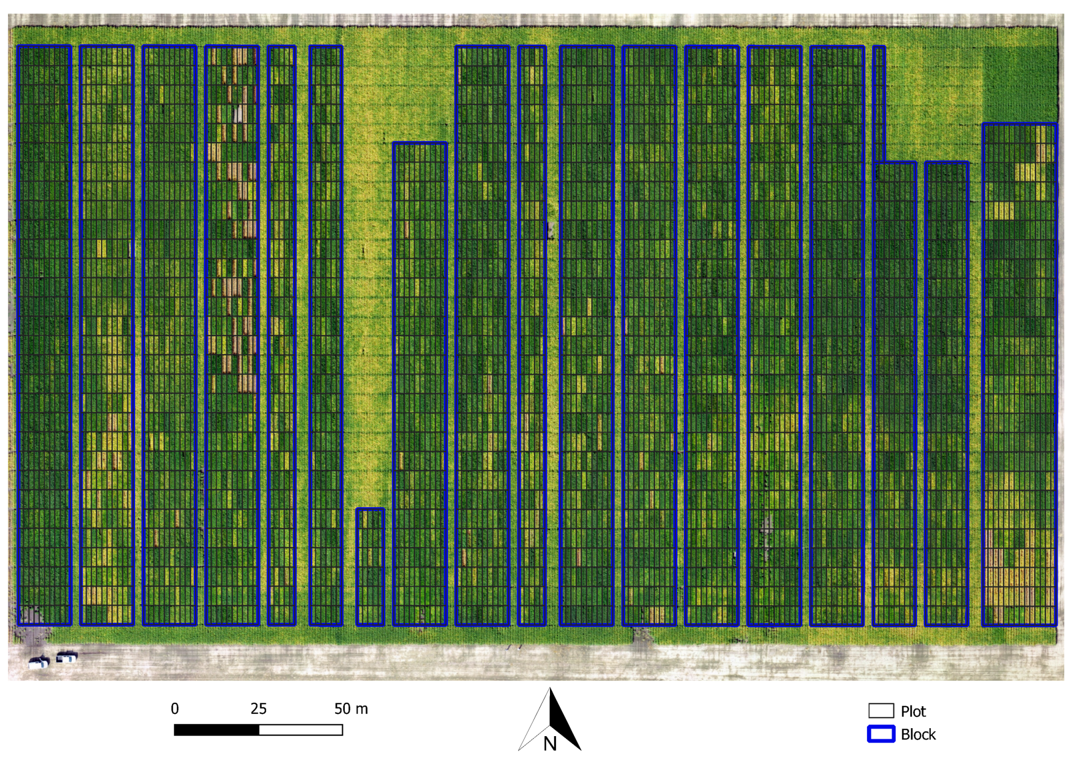
Five trials were conducted in partnership with public and private breeding programs. Each trial was comprised of various blocks with experimental lines in different generations of the selection cycle (Figure 1). A summary of the trials is presented in Table 1. The ground truth maturity date (GTM), equivalent to the R8 phenological stage, was recorded by field visits every three or four days, starting at the end of the growing season when the early lines achieved maturity. About 5% of the plots were used as checks, and for these, the maturity group (MG) was known. Only the plots with GTM were used for training and evaluating the models. The total number of plots is included to allow realistic estimates of image acquisition and storage space requirements for different plot sizes and experiment scales.
2.2. Image Acquisition
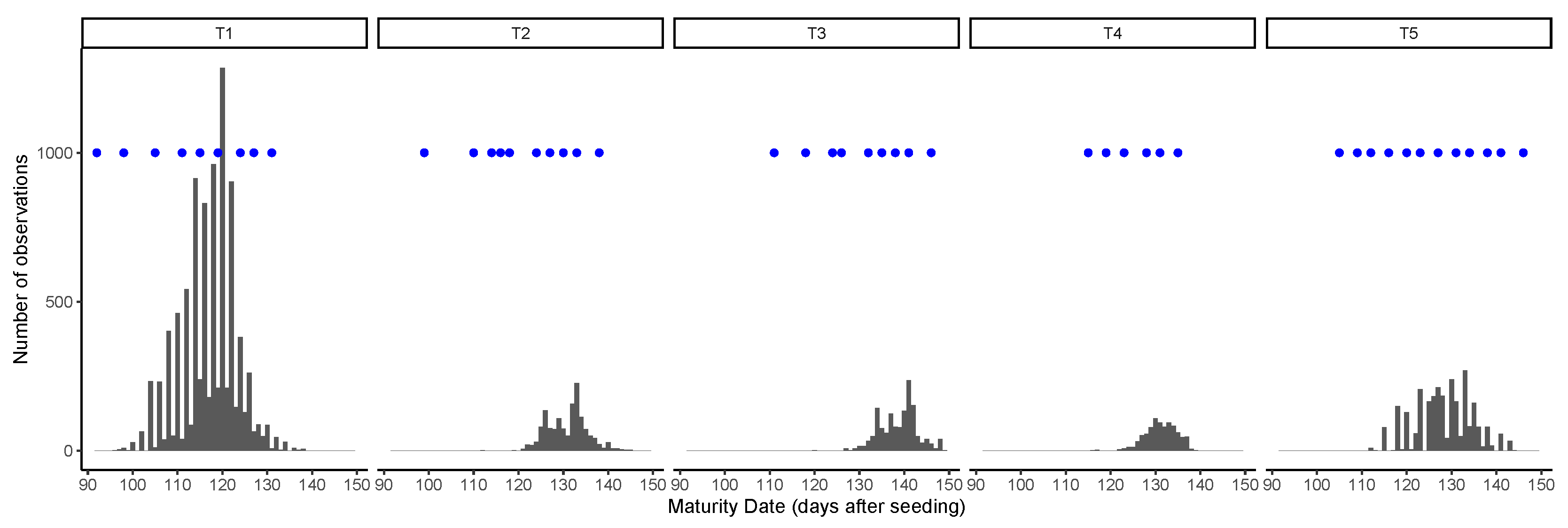
Images were acquired using DJI Phantom 4 Professional UAVs (SZ DJI Technology Co., Ltd., Shenzhen, China), with the built-in 20 MP RGB camera (DJI FC6310) and GPS. The camera has a field of view (FOV) of 84 and an image resolution of 5472 × 3648 pixels, which were stored as JPEG compressed files with an average size of 8 MB. All images were acquired at a flight height of 80 m, yielding a ground sample distance (GSD) of 25 mm/pixel. The image overlap was set to 80% to the front and 60% to the side. The setting up of the flight plan and the acquisition of the images usually took less than one hour, unless there were clouds shading the trials. In such conditions, the flights were paused and resumed. The acquisition of the images followed a similar schedule of the field visits to record GTM data, with about two images per week recorded from the beginning of leaf senescence in the early lines until the latest lines matured (Figure 2). Therefore, the number of flight dates varied according to the range of maturity present in each trial. A summary of the image acquisition step is presented in Table 2.
The reduction in data size from the raw images to the image representing each plot for each date is about 20 times. Half of this reduction came from the areas not occupied by plots, such as the paths and borders. However, the most significant reduction of about ten times is from the elimination of overlaps.
2.3. Image Processing
After the acquisition, the images were processed using the commercial photogrammetry software (Metashape v1.6, Agisoft LLC, St. Petersburg, Russia). The images were matched with the high accuracy setting, followed by the construction of a dense cloud, the digital elevation map, and the orthomosaic. A total of 12 to 18 ground control points (GCPs) were used in each trial. The targets were placed in the field before the first flight and kept in place until the last flight. The coordinates of the markers were extracted from the first date orthomosaic and used in all subsequent dates. In this way, the points are not necessarily globally accurate, but they ensure the temporal consistency of the images. The first image was also used for manual alignment of the trial layout using QGIS software [34]. The georeferenced orthomosaic was exported to a three band (RGB) GeoTIFF file and used to extract the image for each plot using the python packages geopandas and rasterio. Each individual orthophoto was also exported and used to extract replicated observations for each plot.
2.4. Resolution
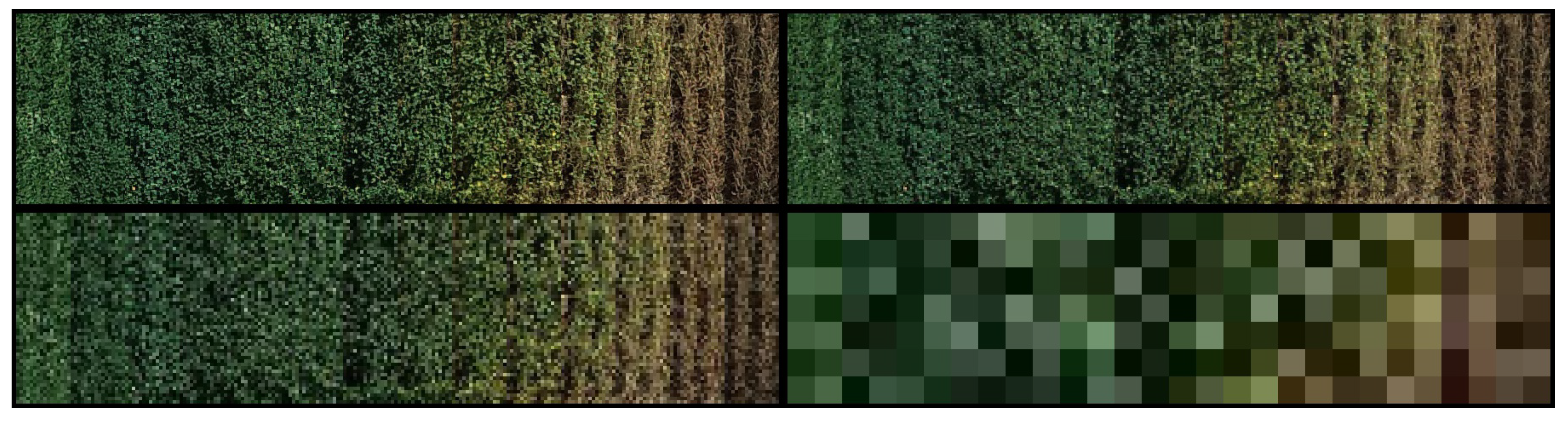
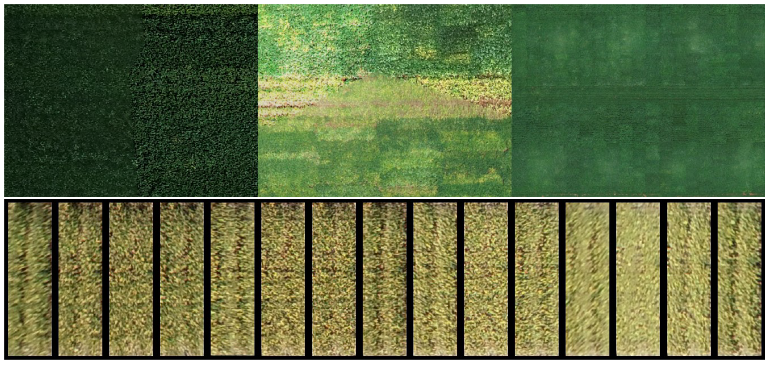
Another important aspect of the images that may affect the model is resolution. Images with downsampled resolution simulating a GSD of 50, 100, and 750 mm/pixel were used to train and compare models. The images were resized accordingly and then compressed to JPEG. For training the model, after decompressing the images, they were scaled back the original resolution in order to use the same model architecture, as illustrated in Figure 3. The visual difference between images with a GSD of 25 and 50 mm/px is very subtle. With 100 mm/px, the difference becomes more evident. The images at 750 mm/px lose all texture information. These were used to help understand the importance of color versus texture and other high-level features.
2.5. Data Augmentation
One of the disadvantages of using low-cost RGB sensors is their sensitivity to variation in light conditions, as observed in Figure 4. This motivated the comparison of different data augmentation strategies to improve the model’s robustness. The first type of image augmentation consisted of digital transformations of the images by applying variation in contrast and luminosity. On the other hand, the availability of many replicates from each plot may be seen as more natural data augmentation. The availability of many replicates can reproduce geometric errors, distortions, blur, and shadow effects that are hard to reproduce with synthetic data augmentation. Therefore, three different strategies of augmentation were compared: no augmentation, synthetic data augmentation, and using the image replicates. At this time, the image digital numbers stored as 8bit integers were converted to 32 bit floats and scaled from the original range (0–255) to have zero mean and unit variance.
2.6. Model Development
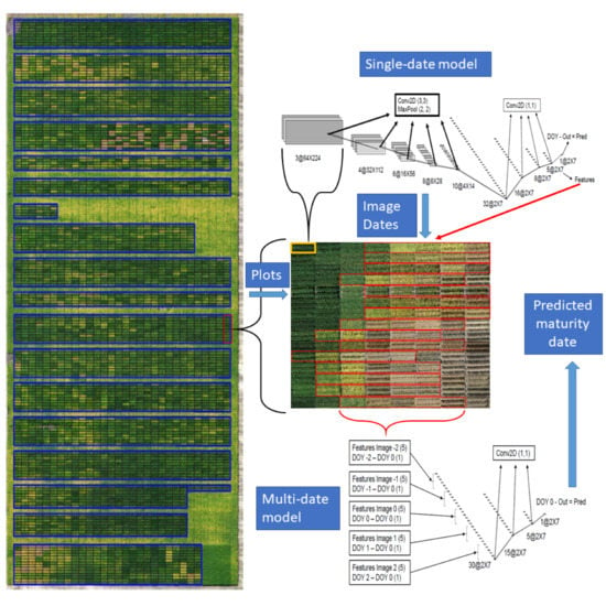
The model was developed with two steps: The architectures used are referred to as single-date (SD) and multi-date (MD) models. In the first step, the model takes one image and predicts the maturity date. The variable ground truth difference (GTDiff), was calculated to represent the difference between the GTM date and the image acquisition date. A set of SD models were trained using 10-fold cross-validation with GTM data for each trial. The predictions in the test set (PREDDiff) were then used to calculate the average root mean squared error (RMSE) for each trial:
where: and are the day of the year in which maturity was predicted and observed, respectively. This allowed the estimation of which GTDiff interval provided the best accuracy in the prediction. The image with the PREDDiff closer to the best GTDiff, and the two images acquired immediately before and after were selected for the next step. The MD model uses the features extracted by the SD at the layer before the predictions, instead of running the model again over the full images, which reduces the number of parameters to be trained. In this way, the SD model, which has more parameters, can be trained with a greater number of observations and data variation, while the MD model only uses a small number of extracted features and few parameters to refine the prediction.
2.7. Single-Date Model Architecture
Based on the layers used and the intention behind their use, the architecture for the SD model can be divided into two groups. In the first group, each block contains a 2D convolution with a 3 × 3 kernels, a max-pooling layer that halves the number of pixels in the output, a dropout layer, and a rectified linear activation function (RELU) activation. The convolutions are zero-padded to keep the output sizes the same as the inputs. This block is repeated sequentially five times. Therefore, the output has its spatial dimensions reduced by a factor of 25 or 32 times. The dimensions shown in Figure 5 are valid for input sizes used in the largest plots. The main purpose of this group of operations is to extract meaningful spatial information and condense it in a lower resolution representation. The next block contains only convolutions with 1 × 1 kernel sizes followed by a dropout layer. Therefore, only the different features of the same pixel are used to calculate the values in the next layer. This block is repeated sequentially four times to obtain the output. The output is then subtracted from the image acquisition date to generate the prediction. This second block does not change the spatial dimension of the output, but it forces the information to be represented by lower-dimensional spaces since the number of channels is being reduced. The result from the layer immediately before the output will be used as features to the temporal model. The reasoning behind the choice to use 1 × 1 convolutions instead of flattening the features was to conserve the variability within the plot to be used in one of the estimates of model uncertainty later. By subtracting the image acquisition date, internally, the model is learning to estimate the difference between the maturity date and the date the image was taken.
2.8. Multi-Date Model Architecture
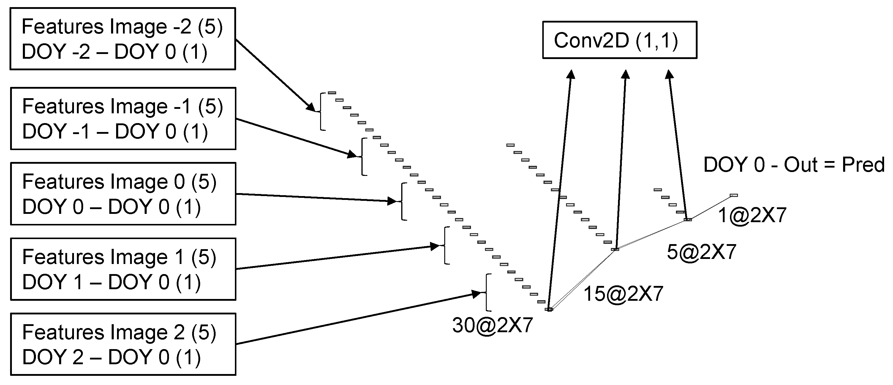
The architecture for the MD model was developed to operate over groups of five images, selected from the results of the SD model. The difference between the day of the year (DOY) of each image and the DOY of the central image was concatenated as an additional feature for each image. The difference date from the center image is always zero and can be omitted. However, it is easier to keep it and have all tensors with the same dimensions. Therefore, six features from each of the five images were concatenated into the 30 features that were used as inputs in the MD model. In case the acquisition dates span through two different years, as happens, for instance, in the South Hemisphere where maturity starts in December, the DOY from the previous year can be negative, or on the contrary, it can be extended beyond 365 for the next year. It is also possible to use days after planting or emergence instead of the day of the year. Because the value is subtracted before entering the model and is added back at the end, it is only the intervals that matter. The architecture used in the MD model is straightforward and follows the same layers of the second block in the single date model Figure 6. To keep the number of parameters to be trained to a minimum, the convolutions with 1 × 1 kernel sizes followed by a dropout layer were repeated sequentially three times. The output is then subtracted from the DOY of the central image to generate the final prediction. The order in which the DOY is subtracted and then added back may not be very intuitive. However, this is necessary to keep the same relationship when the difference is greater because the image was taken earlier or when the soybean line presents delayed maturity.
2.9. Model Parameters
The distribution of the parameters in each step of the model is presented in Table 3. The total number of parameters for the full model was 5682, which characterizes a small and light-weight model, with more observations available than parameters to be estimated. This number is the same independent of the size of the input images. The number of parameters in the SD model was 5131, while the number of parameters in the MD model was 551. The last number represents the effective samples to train the MD model, which is about 10% of the available data to train the SD model.
2.10. Model Training
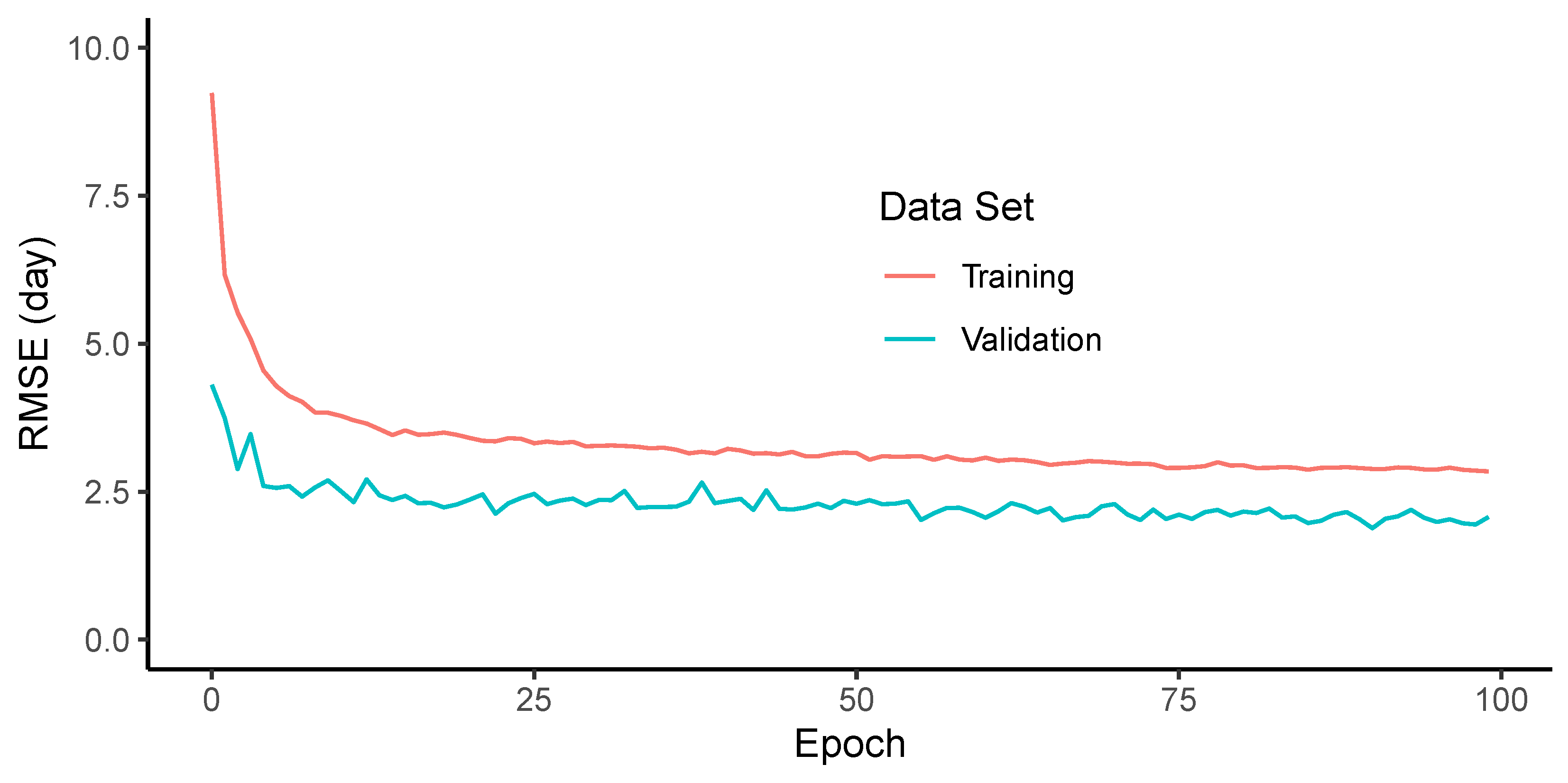
The training and testing were performed in a computer equipped with an Intel i7 processor (Intel Corporation, Santa Clara, CA, USA) and an NVIDIA Quadro P4000 GPU (NVIDIA, Santa Clara, CA, USA) with 8GB memory using the PyTorch deep learning package v. 1.5 [35]. The Adam optimizer, with a learning rate of 0.001 was used. The RMSE was used as the loss function (Equation (1)). The models were trained using 10% dropout rate. The models were trained to a maximum of 100 epochs, using early stopping criteria to monitor the validation set and stop training after the loss did not decrease for 10 consecutive epochs. The architectures and hyper-parameters were fine-tuned based on the amount of data available and the overall results in the validation sets.
2.11. Model Validation
The dataset was split into three different sets used for training, validation, and testing. The validation set is primarily used for early stopping the model. All metrics presented are calculated over the test set. All comparisons were made using 10-fold cross-validation so that all data were evaluated in all sets. The data split was set to 80% for the training set, 10% for the validation set, and 10% for the test set. The split was fully randomized, which represents the most common method used in the literature. The models trained in one trial were also tested in all other trials. Testing in different trials assures more independence of the testing set and reflects a more desirable model.
2.12. Model Uncertainty
In the proposed architecture using only convolutional layers, every 32 × 32 pixels in the input will produce one pixel in the output. The final prediction is taken as the average of the pixels in the prediction. The standard deviation of the predictions is used as an estimate of model uncertainty due to within plot variability. As a consequence of the 10-fold cross-validation, there were ten resulting models for each trial. The standard deviation of these predictions was also evaluated as a metric of uncertainty.
The use of replicated images was also evaluated at test time to estimate the uncertainty caused by variation in light intensity and the overall aspect of the images. This also reflects some of the uncertainty due to the geometric differences in the images, since the distortions are greater for plots close to the borders of the images. Finally, multiple predictions with dropout layers enabled at test time were also used to estimate the uncertainty of the model parameters and architecture. The standard deviation of the predictions with the image replicates, and dropout enabled was computed with 10 random initializations for each plot and method. The four estimates of uncertainty were compared with the average error at a trial level and also correlated to the absolute error of each plot.
3. Results
3.1. Single Date Model
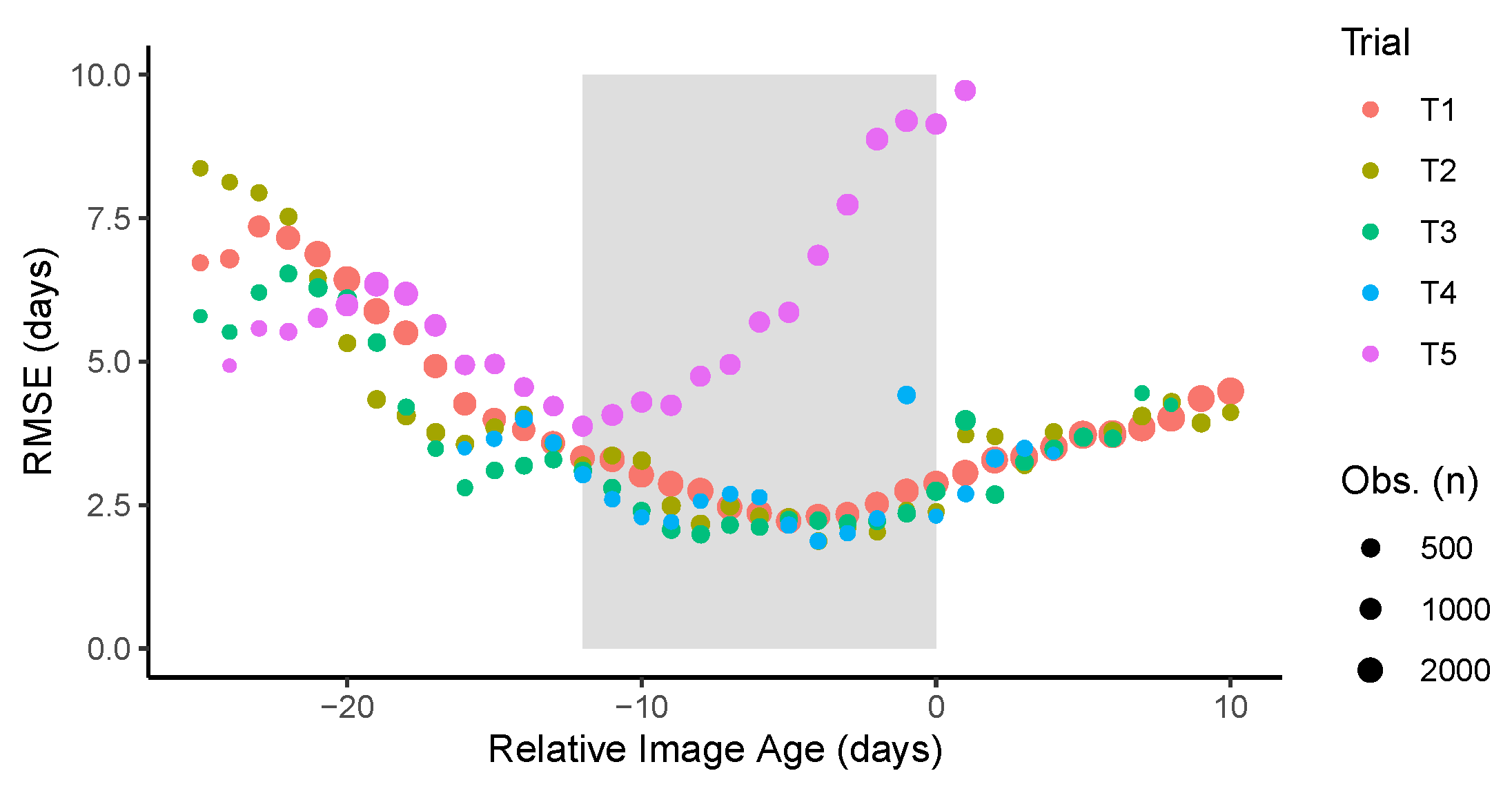
In four of the five trials, the lowest RMSE was observed when the images were acquired about one week before maturity, while for T5 the lowest error was obtained when the images were taken about two weeks prior to maturity (Figure 7). Looking at the images of T5, it was noted that in many plots the plants were lodged on the neighboring plots. Furthermore, it was noted that weed growth occurred simultaneously with the crop senescence, and most importantly, leaf retention after pod senescence. These factors contributed to larger errors when the used images are taken closer to senescence. So, even though under optimal experimental conditions images close to maturity would be preferred, the confounding factors could affect the predicted values and increase the error. When considering all data, the errors remain relatively low for about 12 days before maturity; outside of this range, the errors increase substantially. Based on these observations, the value of the GTDiff was set to −6, meaning that from all the available image dates, the one that predicted maturity would occur about 6 days after the acquisition was used as the center image. The two images acquired immediately before and after this center image usually fell within this 12 day time window. The choice of five images was based mostly on the minimum number of images usually available for the trials. Choosing a fewer number of images may degrade the performance; this is because at prediction time the GTM value is unknown, and the estimates from individual images are used to find the center image. The use of more images confers robustness to the model, in case the choice of images was not optimal.
3.2. Overall Performance
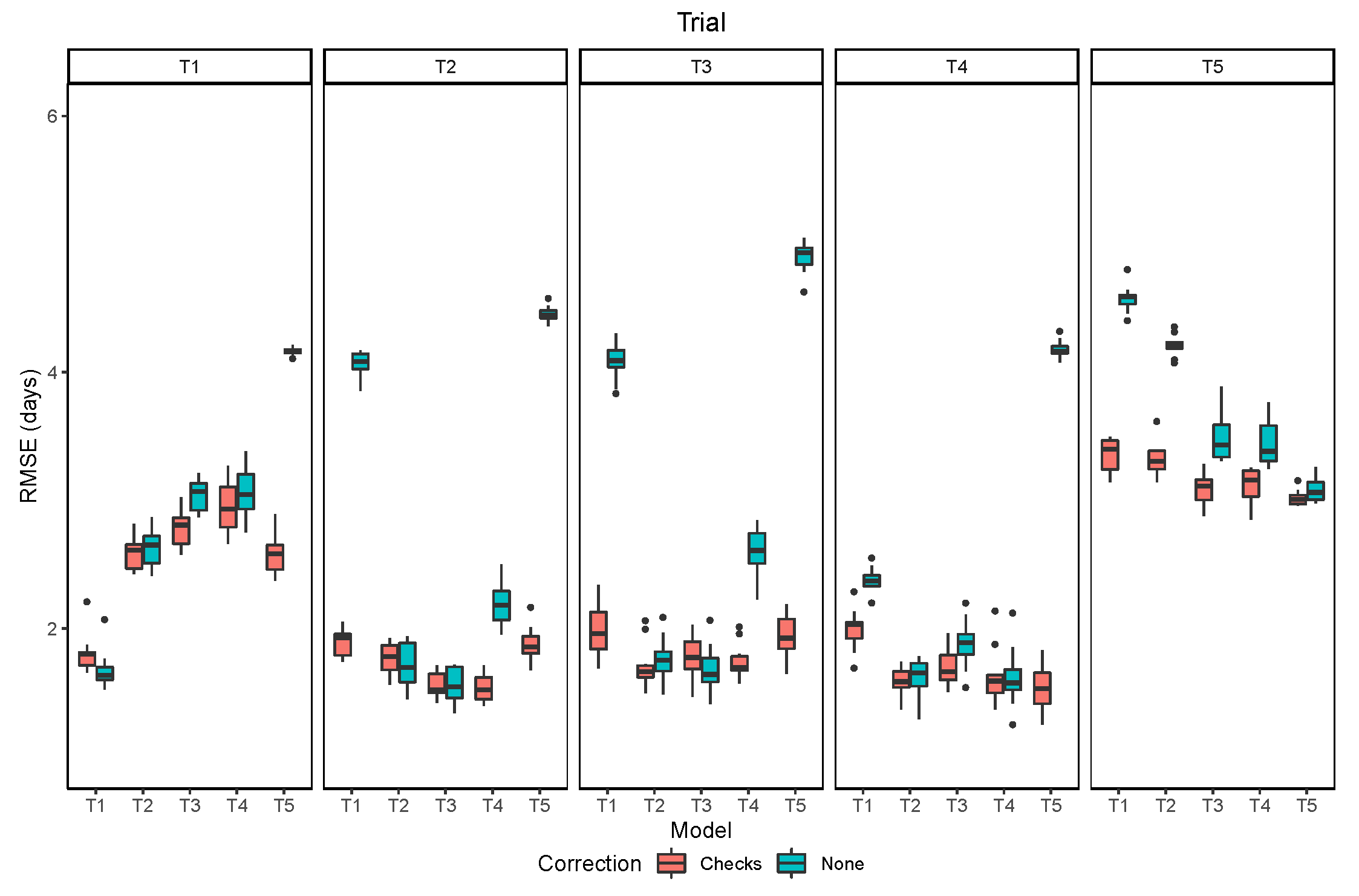
The overall performance of the models trained and evaluated within the same trial indicated an RMSE inferior to 2 days in all trials except T5, in which the RMSE was about 3 days (Figure 8). The lower performance in the last trial is attributed to the lower quality of image acquisition, with more shadows, and to the higher frequency of lines with leaf retention. The performance of models trained in other trials and seasons varied among trials. For most cases with high RMSE there was a bias of a few days in the distributions of predicted and observed values. This could be due to some offset in the relationship of leaf senescence and pod senescence caused by environmental factors and their interaction with the genotype. Part of this bias may also be due to differences in the GTM data acquisition, since the maturity date is an estimate subject to human error. The bias in the raw predictions was corrected using the information from the reference check plots, which greatly reduced the extremely high values of RMSE.
When evaluating the RMSE of the adjusted maturity dates, the models showed good generalization (Figure 9). It can be noted that the number of model parameters and dropout were effective at avoiding overfitting, since the validation loss did not show any trend to increase within the number of epochs used. The RMSE values were lower when the conditions were similar, but the increased errors when the conditions of the trial changed. For example, all models performed well in trials T2, T3 and T4, which had good quality images and no confounding factors in the trial. However, all the models that were trained in other trials, had higher errors in T1. One reason for that was due to the emergence of a new generation of seedlings after the harvest of the earlier maturing lines. This caused some plots to be green again in the last two acquisition dates. Even though this effect added a low error, considering that the predictions in the single date model were good enough to choose the early images, under other conditions, few large errors could cause an overall increase in the RMSE.
3.3. Resolution
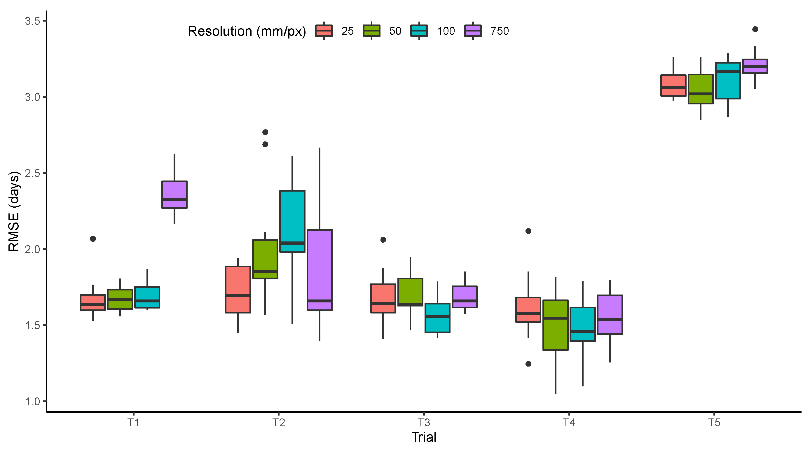
The effect of resolution was small, resulting in similar model performance in most trials with variations between 25 and 100 mm/px (Figure 10). The most significant increase in the RMSE was observed in T1 with the lowest resolution (750 mm/px). This shows that the features learned by the model in T1 depend on the texture of images and not only on the color. For the other trials, the small differences may be related to the number of observations used to train the model, which were five to 10 times fewer than what was available for T1. The trials in which the quality of resolution was less important also had more problems with out of focus images such as the examples shown earlier (Figure 4). It is also important to note that even with the best resolution (25 mm/px), the pods cannot be distinguished from the leaves, which would be necessary to improve the models when germplasm expressing leaf retention is present in the trials.
3.4. Data Augmentation
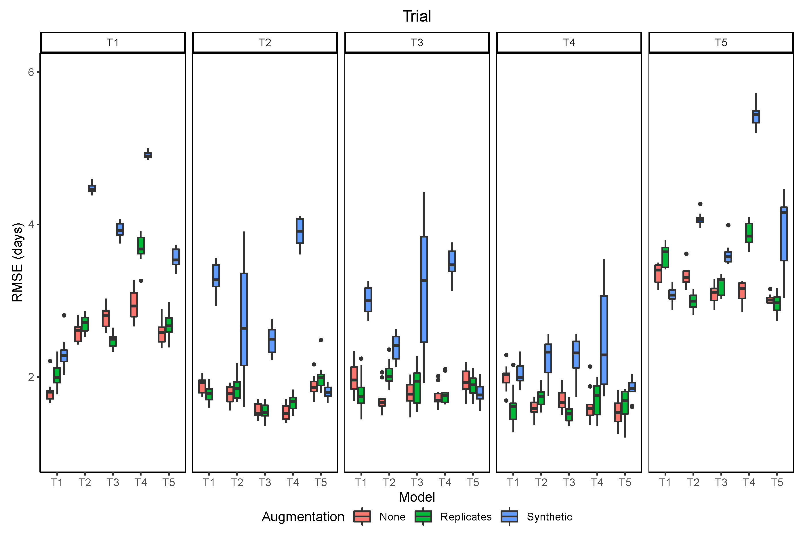
The two strategies of data augmentation used to train the models did not improve the results, compared to no data augmentation (Figure 11). Overall, the use of synthetic augmentation decreased model performance when it was evaluated at the same trial, and even more, when it was evaluated in the other trials. The use of the image replicates had mixed results, with increased generalization when the model was tested in other trials in a few cases, but with decreased performance being still more frequent. These results give further evidence to what was observed from the image resolution analysis. Since the model relies mostly on the average color of each image, applying augmentation techniques that change the color of the images (brightness, contrast), leads to a decrease of the model accuracy. In contrast, the augmentation technique has had more success in other computer vision problems, where more complex features related to image texture and shape of objects are more important than color.
3.5. Uncertainty
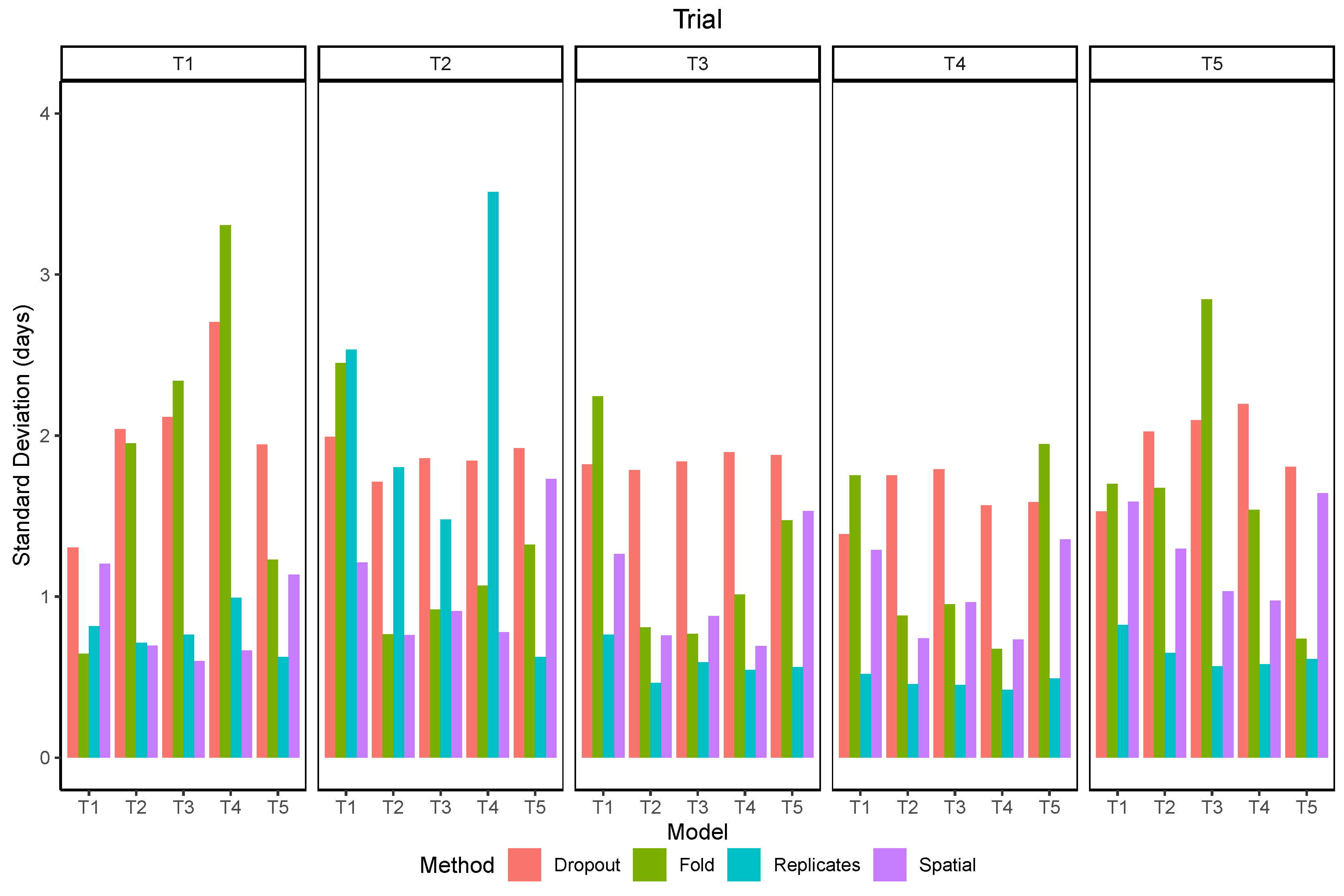
The standard deviation of the within-plot predictions (spatial) was more related to the data used for training than the trial in which the predictions were made (Figure 12). The values were lower than 1 day for models trained in trials with bigger plots and higher than 1 day for the models trained in T1 and T5. The standard deviation of using models trained with different subsets of the data (folds) shows a clear difference towards lower RMSE when the model included data from the same trial and when it did not. There was also a distinction of two groups of trials, as models trained in T2, T3, or T4 had lower variation when tested within this group but higher values when tested in T1 or T5, and vice-versa. The standard deviation of using image replicates was lower than 1 day for all trials except in T2, for which its values were higher than the uncertainty estimated by other methods. The standard deviation of predictions with dropout layers enabled was usually higher than the other methods, but similar for all trials and models.
The correlations between the standard deviation of predictions and the absolute error varied from −0.1 to 0.3 depending on the trial and the model (Figure 13). In most scenarios the correlation was positive, although some negative values were observed, mostly when using dropout. The overall correlation was higher in T1 and lower in T2, independently of the method. Using dropout presented mixed results, with the best correlation when the model trained in T2 was used in T3. Using the replicates produced the best results in T1 and T5.
4. Discussion
The maturity prediction was framed as a regression model, aiming to predict the maturity date as a continuous variable, instead of classifying each plant row as mature or immature for a given date [15]. This eliminates the need for post-processing steps before getting the final result. It also makes it easy to include local information from the check plots in a simple linear regression to account for the environmental factors and assign the maturity group. Reporting the results in terms of the RMSE enables a better evaluation of the model than using classification accuracy, as images taken far from the maturity date are easier to classify but do not contribute to improved model performance.
The overall performance of the model was superior to what has been reported in previous studies. One study, using partial least square regression (PLSR) and three vegetation indices to predict maturity in a diverse set of soybean genotypes, achieved an RMSE of 5.19 days [36]. Another recent study, also using PLSR models and 130 handcrafted features from five-band multispectral images, achieved an RMSE of 1.4 days [26]. However, this study used 326 GTM observations with a range of maturity dates of only 10 days, which makes low RMSE easier to achieve. The relatively low importance of image resolution, which is an indicator of the importance of using CNN as feature extractors, shows that this was not the main reason to explain the good performance of the model.
The CNN model is able to learn how to extract the best combination of features. This flexibility would allow using the model for the extraction of many traits of interest at the same time. For example, the same model could be trained to predict maturity date, senescence rate, lodging and pubescence color. The importance of image resolution and the automated feature extraction with CNNs was demonstrated in a similar study in rice [32]. In that study, the accuracy of the phenological stages estimation was higher with image resolutions of 20–40 mm/px and decreased sharply when they were reduced to 80–160 mm/px. The maturity in rice is observed in the panicles, which are at the top of the canopy, more visible in the images than the soybean pods, which are in the middle of the canopy. Therefore, it is likely that the best resolution tested in this work (25 mm/px) is still too coarse to allow the model to learn any feature specific to the pods, which is an explanation for why there was little impact of reductions in resolution. A future research direction could be to evaluate the importance of much higher resolutions, which could be obtained with lower flying altitudes or using autonomous ground vehicles [37].
Contrary to the expected, using replicated observations from different images of the same plot did not increase the model performance. More surprising, applying synthetic data augmentation markedly decreased the model performance in most cases. This result is mostly attributed to the relative importance of color, rather than more complex plant features. Another reason for the low performance when using augmentation may be the simultaneous use of dropout. Some works have shown that for most models there is an equivalence between dropout and data augmentation [38], both introducing some randomness to reduce the risk of overfitting. Since dropout was used in all models, it is possible that the combination of dropout and data augmentation created excessive randomness, reducing the effectiveness of the model training. Considering that dropout is easier to implement and does not require assumptions about what types of augmentation are meaningful, this would be preferred instead of data augmentation. However, a more thorough evaluation of hyper-parameters could be done in future research to confirm these findings.
Developing a model with low prediction error using RGB images makes it more likely to be used due to the low cost. Besides, an RMSE of about 1.5 to 2.0 days is usually considered the acceptable limit in breeding programs [26]. Considering that errors above this limit were observed in T5, the use of multispectral images could provide better results when leaf retention is a significant concern. The challenge to correctly predict maturity in plots where plants with mature pods still retain green leaves has been previously reported [15]. This type of error is more important than a random error because some lines consistently would have higher errors than others, possibly affecting the selection decisions. Future works to predict physiological maturity should consider foliar retention as a trait to be analyzed. Another consideration is what stage should maturities be predicted or visually rated in breeding programs. Breeders will develop and test tens of thousands of experimental lines annually and evaluate them in small plots. It is very labor-intensive to evaluate all of these lines visually for maturity, and it is not critically important to obtain accurate maturity estimates at this stage as the estimates are used to place lines in tests with similar maturities. Predicting maturities with a UAV would most benefit breeding programs at this stage. At later stages of breeding programs, more accurate estimates are needed so that the maturity groups of cultivars can be determined.
One particularity of the proposed architecture is the use of only convolutional layers instead of using fully connected layers for the final prediction. Although this is common in semantic segmentation tasks, it is less used for regression tasks. The goal of applying this strategy in this context was also different. Rather than improving performance, the main purpose was to add flexibility and to estimate prediction uncertainty due to within plot variability. This was demonstrated in Figure 13, and was helpful to identify the sources of prediction errors in some plots (Figure 14). In a similar way, the use of image replicates also identified an overall higher uncertainty in T2 and was positively correlated with errors of individual plots in T1. Therefore, the different methods of uncertainty estimation can be used for two different purposes. The first is to evaluate the overall quality of the images and procedures used at the trial level, which can identify problems with image stitching or radiometric calibration. The second use is to select individual plots in which the error is likely to be higher, which should be targeted for new data acquisition in order to improve the model.
Another source of uncertainty comes from the imprecision of GTM ratings, and is related to the observation frequency, the experience level of the people collecting the data, and the number of people taking notes for the same field. In order to estimate this source of uncertainty it would be necessary to conduct independent maturity assessments by different people in the the same plots with a higher frequency of field visits, ideally daily. This is beyond the scope of this work, and is left as a suggestion for future research.
Most of the processing time is spent preparing the images for each plot and training the models, but making the predictions is actually very fast. With more than one thousand predictions per second, in the hardware used, using the GPU, this shows the potential scalability of the method once other bottlenecks in image processing are solved. Fast predictions are also important to enable the test time augmentation and evaluate the model uncertainty. The ability to understand when the predictions fail is one of the foundations for model improvement. This also opens the possibility of using model ensembles to improve predictions and to better identify the uncertainty [39].
5. Conclusions
The strategy of choosing a subset of images that contribute the most to model accuracy proved to be successful in conferring flexibility to the model. Models trained in other trials and years, with different plot sizes and image acquisition intervals, were able to predict soybean maturity date with an RMSE lower than 2.0 days in four out of five trials. Compared to previous studies, additional challenges were addressed, focusing on the scalability of the proposed solutions. This was possible after using more than 15,000 ground truth maturity date observations from five trials, including data from three growing seasons and two countries. Data augmentation did not improve model performance and was harmful in many cases. Changing the resolution of images did not affect model performance. Model performance decreased when tested in trials with conditions unseen during training. Using ground truth information from check plots helped to correct for environmental bias. Four methods of estimating prediction uncertainty showed potential at identifying different sources of errors in the maturity date predictions. The main challenge remaining to improve model accuracy is the low correlation between leaf senescence and pod senescence for some genotypes.
Author Contributions
Conceptualization, R.T., O.P., B.D., N.S. and N.M.; Methodology, R.T. and N.M.; Software, R.T.; Validation, R.T., O.P. and B.D.; Formal Analysis, R.T.; Investigation, O.P., B.D. and N.S.; Resources, B.D., N.S. and N.M.; Data Curation, R.T., O.P., B.D. and N.S.; Writing—Original Draft Preparation, R.T.; Writing—Review and Editing, R.T., O.P., B.D. and N.M.; Visualization, R.T.; Supervision, B.D. and N.M.; Project Administration, N.M.; Funding Acquisition, B.D. and N.M. All authors have read and agreed to the published version of the manuscript.
Funding
This research received no external funding.
Acknowledgments
To the Don Mario Group (GDM Seeds) for providing the images and part of the ground truth maturity data used in this work.
Conflicts of Interest
The authors declare no conflict of interest.
References
- Hartman, G.L.; West, E.D.; Herman, T.K. Crops that feed the World 2. Soybean—Worldwide production, use, and constraints caused by pathogens and pests. Food Secur. 2011, 3, 5–17. [Google Scholar] [CrossRef]
- Liu, S.; Zhang, M.; Feng, F.; Tian, Z. Toward a “Green Revolution” for Soybean. Mol. Plant 2020, 13, 688–697. [Google Scholar] [CrossRef]
- Cobb, J.N.; DeClerck, G.; Greenberg, A.; Clark, R.; McCouch, S. Next-generation phenotyping: requirements and strategies for enhancing our understanding of genotype—Phenotype relationships and its relevance to crop improvement. Theor. Appl. Genet. 2013, 126, 867–887. [Google Scholar] [CrossRef] [PubMed] [Green Version]
- Moreira, F.F.; Hearst, A.A.; Cherkauer, K.A.; Rainey, K.M. Improving the efficiency of soybean breeding with high-throughput canopy phenotyping. Plant Methods 2019, 15, 139. [Google Scholar] [CrossRef]
- Morales, N.; Kaczmar, N.S.; Santantonio, N.; Gore, M.A.; Mueller, L.A.; Robbins, K.R. ImageBreed: Open-access plant breeding web–database for image-based phenotyping. Plant Phenome J. 2020, 3, 1–7. [Google Scholar] [CrossRef]
- Reynolds, M.; Chapman, S.; Crespo-Herrera, L.; Molero, G.; Mondal, S.; Pequeno, D.N.; Pinto, F.; Pinera-Chavez, F.J.; Poland, J.; Rivera-Amado, C.; et al. Breeder friendly phenotyping. Plant Sci. 2020. [Google Scholar] [CrossRef]
- Fehr, W.; Caviness, C.; Burmood, D.; Pennington, J. Stage of soybean development. Spec. Rep. 1977, 80, 929–931. [Google Scholar]
- Koga, L.J.; Canteri, M.G.; Calvo, E.S.; Martins, D.C.; Xavier, S.A.; Harada, A.; Kiihl, R.A.S. Managing soybean rust with fungicides and varieties of the early/semi-early and intermediate maturity groups. Trop. Plant Pathol. 2014, 39, 129–133. [Google Scholar] [CrossRef] [Green Version]
- Andrea, M.C.d.S.; Dallacort, R.; Tieppo, R.C.; Barbieri, J.D. Assessment of climate change impact on double-cropping systems. SN Appl. Sci. 2020, 2, 1–13. [Google Scholar] [CrossRef] [Green Version]
- Alliprandini, L.F.; Abatti, C.; Bertagnolli, P.F.; Cavassim, J.E.; Gabe, H.L.; Kurek, A.; Matsumoto, M.N.; De Oliveira, M.A.R.; Pitol, C.; Prado, L.C.; et al. Understanding soybean maturity groups in brazil: Environment, cultivar classifi cation, and stability. Crop Sci. 2009, 49, 801–808. [Google Scholar] [CrossRef]
- Song, W.; Sun, S.; Ibrahim, S.E.; Xu, Z.; Wu, H.; Hu, X.; Jia, H.; Cheng, Y.; Yang, Z.; Jiang, S.; et al. Standard Cultivar Selection and Digital Quantification for Precise Classification of Maturity Groups in Soybean. Crop Sci. 2019, 59, 1997–2006. [Google Scholar] [CrossRef] [Green Version]
- Mourtzinis, S.; Conley, S.P. Delineating soybean maturity groups across the United States. Agron. J. 2017, 109, 1397–1403. [Google Scholar] [CrossRef] [Green Version]
- Zdziarski, A.D.; Todeschini, M.H.; Milioli, A.S.; Woyann, L.G.; Madureira, A.; Stoco, M.G.; Benin, G. Key soybean maturity groups to increase grain yield in Brazil. Crop Sci. 2018, 58, 1155–1165. [Google Scholar] [CrossRef]
- Araus, J.L.; Kefauver, S.C.; Zaman-Allah, M.; Olsen, M.S.; Cairns, J.E. Translating High-Throughput Phenotyping into Genetic Gain. Trends Plant Sci. 2018, 23, 451–466. [Google Scholar] [CrossRef] [Green Version]
- Yu, N.; Li, L.; Schmitz, N.; Tian, L.F.; Greenberg, J.A.; Diers, B.W. Development of methods to improve soybean yield estimation and predict plant maturity with an unmanned aerial vehicle based platform. Remote Sens. Environ. 2016, 187, 91–101. [Google Scholar] [CrossRef]
- Yang, G.; Liu, J.; Zhao, C.; Li, Z.; Huang, Y.; Yu, H.; Xu, B.; Yang, X.; Zhu, D.; Zhang, X.; et al. Unmanned aerial vehicle remote sensing for field-based crop phenotyping: Current status and perspectives. Front. Plant Sci. 2017, 8. [Google Scholar] [CrossRef]
- Reynolds, D.; Baret, F.; Welcker, C.; Bostrom, A.; Ball, J.; Cellini, F.; Lorence, A.; Chawade, A.; Khafif, M.; Noshita, K.; et al. What is cost-efficient phenotyping? Optimizing costs for different scenarios. Plant Sci. 2019, 282, 14–22. [Google Scholar] [CrossRef] [Green Version]
- Borra-Serrano, I.; De Swaef, T.; Quataert, P.; Aper, J.; Saleem, A.; Saeys, W.; Somers, B.; Roldán-Ruiz, I.; Lootens, P. Closing the Phenotyping Gap: High Resolution UAV Time Series for Soybean Growth Analysis Provides Objective Data from Field Trials. Remote Sens. 2020, 12, 1644. [Google Scholar] [CrossRef]
- Tsaftaris, S.A.; Minervini, M.; Scharr, H. Machine Learning for Plant Phenotyping Needs Image Processing. Trends Plant Sci. 2016, 21, 989–991. [Google Scholar] [CrossRef] [Green Version]
- Schnaufer, C.; Pistorius, J.L.; LeBauer, D. An open, scalable, and flexible framework for automated aerial measurement of field experiments. In Autonomous Air and Ground Sensing Systems for Agricultural Optimization and Phenotyping V; Thomasson, J.A., Torres-Rua, A.F., Eds.; SPIE: Bellingham, WA, USA, 2020; p. 9. [Google Scholar] [CrossRef]
- Ampatzidis, Y.; Partel, V.; Costa, L. Agroview: Cloud-based application to process, analyze and visualize UAV-collected data for precision agriculture applications utilizing artificial intelligence. Comput. Electron. Agric. 2020, 174, 105457. [Google Scholar] [CrossRef]
- Matias, F.I.; Caraza-Harter, M.V.; Endelman, J.B. FIELDimageR: An R package to analyze orthomosaic images from agricultural field trials. Plant Phenome J. 2020, 3, 1–6. [Google Scholar] [CrossRef]
- Khan, Z.; Miklavcic, S.J. An Automatic Field Plot Extraction Method From Aerial Orthomosaic Images. Front. Plant Sci. 2019, 10, 1–13. [Google Scholar] [CrossRef]
- Tresch, L.; Mu, Y.; Itoh, A.; Kaga, A.; Taguchi, K.; Hirafuji, M.; Ninomiya, S.; Guo, W. Easy MPE: Extraction of Quality Microplot Images for UAV-Based High-Throughput Field Phenotyping. Plant Phenomics 2019, 2019, 1–9. [Google Scholar] [CrossRef] [Green Version]
- Chen, C.J.; Zhang, Z. GRID: A Python Package for Field Plot Phenotyping Using Aerial Images. Remote Sens. 2020, 12, 1697. [Google Scholar] [CrossRef]
- Zhou, J.J.; Yungbluth, D.; Vong, C.N.; Scaboo, A.; Zhou, J.J. Estimation of the Maturity Date of Soybean Breeding Lines Using UAV-Based Multispectral Imagery. Remote Sens. 2019, 11, 2075. [Google Scholar] [CrossRef] [Green Version]
- Jiang, Y.; Li, C. Convolutional Neural Networks for Image-Based High-Throughput Plant Phenotyping: A Review. Plant Phenomics 2020, 2020, 1–22. [Google Scholar] [CrossRef] [Green Version]
- Dobrescu, A.; Giuffrida, M.V.; Tsaftaris, S.A. Doing More With Less: A Multitask Deep Learning Approach in Plant Phenotyping. Front. Plant Sci. 2020, 11, 1–11. [Google Scholar] [CrossRef]
- David, E.; Madec, S.; Sadeghi-Tehran, P.; Aasen, H.; Zheng, B.; Liu, S.; Kirchgessner, N.; Ishikawa, G.; Nagasawa, K.; Badhon, M.A.; et al. Global Wheat Head Detection (GWHD) dataset: A large and diverse dataset of high resolution RGB labelled images to develop and benchmark wheat head detection methods. arXiv 2020, arXiv:2005.02162. [Google Scholar]
- Maimaitijiang, M.; Sagan, V.; Sidike, P.; Hartling, S.; Esposito, F.; Fritschi, F.B. Soybean yield prediction from UAV using multimodal data fusion and deep learning. Remote Sens. Environ. 2020, 237, 111599. [Google Scholar] [CrossRef]
- Yuan, W.; Wijewardane, N.K.; Jenkins, S.; Bai, G.; Ge, Y.; Graef, G.L. Early Prediction of Soybean Traits through Color and Texture Features of Canopy RGB Imagery. Sci. Rep. 2019, 9, 14089. [Google Scholar] [CrossRef] [Green Version]
- Yang, Q.; Shi, L.; Han, J.; Yu, J.; Huang, K. A near real-time deep learning approach for detecting rice phenology based on UAV images. Agric. For. Meteorol. 2020, 287, 107938. [Google Scholar] [CrossRef]
- Wang, X.; Xuan, H.; Evers, B.; Shrestha, S.; Pless, R.; Poland, J. High-throughput phenotyping with deep learning gives insight into the genetic architecture of flowering time in wheat. GigaScience 2019, 8, 1–11. [Google Scholar] [CrossRef]
- QGIS Development Team. QGIS Geographic Information System Software, Version 3.10; Open Source Geospatial Foundation: Beaverton, OR, USA, 2020. [Google Scholar]
- Paszke, A.; Gross, S.; Massa, F.; Lerer, A.; Bradbury, J.; Chanan, G.; Killeen, T.; Lin, Z.; Gimelshein, N.; Antiga, L.; et al. PyTorch: An Imperative Style, High-Performance Deep Learning Library. In Proceedings of the Advances in Neural Information Processing Systems, Vancouver, BC, Canada, 8–14 December 2019; pp. 8026–8037. [Google Scholar]
- Christenson, B.S.; Schapaugh, W.T.; An, N.; Price, K.P.; Prasad, V.; Fritz, A.K. Predicting soybean relative maturity and seed yield using canopy reflectance. Crop Sci. 2016, 56, 625–643. [Google Scholar] [CrossRef] [Green Version]
- Young, S.N.; Kayacan, E.; Peschel, J.M. Design and field evaluation of a ground robot for high-throughput phenotyping of energy sorghum. Precis. Agric. 2019, 20, 697–722. [Google Scholar] [CrossRef] [Green Version]
- Zhao, D.; Yu, G.; Xu, P.; Luo, M. Equivalence between dropout and data augmentation: A mathematical check. Neural Netw. 2019, 115, 82–89. [Google Scholar] [CrossRef] [PubMed]
- Lakshminarayanan, B.; Pritzel, A.; Blundell, C. Simple and scalable predictive uncertainty estimation using deep ensembles. In Proceedings of the Advances in Neural Information Processing Systems, Long Beach, LA, USA, 4–9 December 2017; pp. 6402–6413. [Google Scholar]
Figure 1.
Example of soybean breeding field trial (T4) with layout of plots overlaid on top of the UAV mosaic from images acquired 112 days after seeding.
Figure 1.
Example of soybean breeding field trial (T4) with layout of plots overlaid on top of the UAV mosaic from images acquired 112 days after seeding.

Figure 2.
Distribution of ground truth maturity dates and image acquisition dates (blue dots) in each trial.
Figure 2.
Distribution of ground truth maturity dates and image acquisition dates (blue dots) in each trial.

Figure 3.
Time series of plot images with resolution of 25 mm/px (top left), 50 mm/px (top right), 100 mm/px (bottom left), and 750 mm/px (bottom right).
Figure 3.
Time series of plot images with resolution of 25 mm/px (top left), 50 mm/px (top right), 100 mm/px (bottom left), and 750 mm/px (bottom right).

Figure 4.
Examples of image variations caused by shadows, out of focus images and direct reflection of sunlight (top), and differences found among replicated images of the same plot (bottom).
Figure 4.
Examples of image variations caused by shadows, out of focus images and direct reflection of sunlight (top), and differences found among replicated images of the same plot (bottom).

Figure 5.
Schematic representation of the single date convolutional neural network architecture. The numbers represent the dimensions of the tensors and the names in the boxes are the operations applied. DOY stands for the day of the year.
Figure 5.
Schematic representation of the single date convolutional neural network architecture. The numbers represent the dimensions of the tensors and the names in the boxes are the operations applied. DOY stands for the day of the year.

Figure 6.
Schematic representation of the multi date convolutional neural network architecture. The numbers represent the dimensions of the tensors and the names in the boxes are the operations applied. The DOY stands for the day of year.
Figure 6.
Schematic representation of the multi date convolutional neural network architecture. The numbers represent the dimensions of the tensors and the names in the boxes are the operations applied. The DOY stands for the day of year.

Figure 7.
Prediction performance measured by the root mean squared error (RMSE) as a function of the difference between the image acquisition date and the ground truth maturity date. The shaded area represents the time window comprising the five images with the least error.
Figure 7.
Prediction performance measured by the root mean squared error (RMSE) as a function of the difference between the image acquisition date and the ground truth maturity date. The shaded area represents the time window comprising the five images with the least error.

Figure 8.
Prediction performance measured by the root mean squared error (RMSE) for the raw model outputs and after the correction using the check plots.
Figure 8.
Prediction performance measured by the root mean squared error (RMSE) for the raw model outputs and after the correction using the check plots.

Figure 9.
Prediction performance measured by the root mean squared error (RMSE) as a function of the number of iterations (epochs) for the training and validation data sets.
Figure 9.
Prediction performance measured by the root mean squared error (RMSE) as a function of the number of iterations (epochs) for the training and validation data sets.

Figure 10.
Prediction performance measured by the root mean squared error (RMSE) as related to simulated image resolutions.
Figure 10.
Prediction performance measured by the root mean squared error (RMSE) as related to simulated image resolutions.

Figure 11.
Prediction performance measured by the root mean squared error (RMSE) as related to different data augmentation strategies.
Figure 11.
Prediction performance measured by the root mean squared error (RMSE) as related to different data augmentation strategies.

Figure 12.
Standard deviation of maturity predictions using different methods to estimate uncertainty.
Figure 12.
Standard deviation of maturity predictions using different methods to estimate uncertainty.

Figure 13.
Correlation between the standard deviation and the absolute error of maturity predictions using different methods to estimate uncertainty.
Figure 13.
Correlation between the standard deviation and the absolute error of maturity predictions using different methods to estimate uncertainty.

Figure 14.
Examples of replicated images from trial T5 illustrating leaf retention, weeds and influence from neighboring plots.
Figure 14.
Examples of replicated images from trial T5 illustrating leaf retention, weeds and influence from neighboring plots.


Table 1.
Field trials from different breeding programs used for data collection.
| Trial | Year | Location | Plot Length (m) | Plot Width (m) | #Plot * | #GTM * |
|---|---|---|---|---|---|---|
| T1 | 2018 | Savoy, IL-USA | 2.20 | 1 × 0.76 | 9360 | 9230 |
| T2 | 2019 | Champaign, IL-USA | 5.50 | 2 × 0.76 | 8608 | 1421 |
| T3 | 2019 | Arcola, IL-USA | 5.50 | 2 × 0.76 | 6272 | 1408 |
| T4 | 2019 | Litchfield, IL-USA | 5.50 | 2 × 0.76 | 6400 | 883 |
| T5 | 2019 | Rolândia, PR-Brazil | 5.50 | 2 × 0.50 | 7170 | 2680 |
* #Plot: total number of plots in the trial; #GTM: number of plots with ground truth maturity date observations.
Table 2.
Image acquisition details and total storage used for each breeding trial.
| Trial | Images | Dates | Height (px/plot) | Width (px/plot) | Raw Data (GB) | Processed Data (GB) |
|---|---|---|---|---|---|---|
| T1 | 100 | 9 | 32 | 96 | 7.2 | 0.10 |
| T2 | 250 | 10 | 64 | 224 | 20.0 | 0.53 |
| T3 | 150 | 9 | 64 | 224 | 10.8 | 0.32 |
| T4 | 200 | 6 | 64 | 224 | 9.6 | 0.22 |
| T5 | 200 | 12 | 40 | 224 | 19.2 | 0.30 |
Table 3.
Details of model architecture and number of parameters in each layer.
| Layer | Kernel Dim | Tensor Shape | Param # |
|---|---|---|---|
| Conv2D-S1 | [3,3,3] | [−1, 3, h, w] | 112 |
| Conv2D-S2 | [4,3,3] | [−1, 4, h/2, w/2] | 222 |
| Conv2D-S3 | [6,3,3] | [−1, 6, h/4, w/4] | 440 |
| Conv2D-S4 | [8,3,3] | [−1, 8, h/8, w/8] | 730 |
| Conv2D-S5 | [10,3,3] | [−1, 10, h/16, w/16] | 2912 |
| Conv2D-S6 | [32,1,1] | [−1, 32, h/32, w/32] | 528 |
| Conv2D-S7 | [16,1,1] | [−1, 16, h/32, w/32] | 136 |
| Conv2D-S8 | [8,1,1] | [−1, 8, h/32, w/32] | 45 |
| Conv2D-S9 | [5,1,1] | [−1, 5, h/32, w/32] | 6 |
| Total Single | [−1, 1, h/32, w/32] | 5131 | |
| Conv2D-M1 | [30,1,1] | [−1, 30, h/32, w/32] | 465 |
| Conv2D-M2 | [15,1,1] | [−1, 15, h/32, w/32] | 80 |
| Conv2D-M3 | [5,1,1] | [−1, 5, h/32, w/32] | 6 |
| Total Multi | [−1, 1, h/32, w/32] | 551 | |
| Total | 5682 |
Publisher’s Note: MDPI stays neutral with regard to jurisdictional claims in published maps and institutional affiliations. |
© 2020 by the authors. Licensee MDPI, Basel, Switzerland. This article is an open access article distributed under the terms and conditions of the Creative Commons Attribution (CC BY) license (http://creativecommons.org/licenses/by/4.0/).
Share and Cite
MDPI and ACS Style
Trevisan, R.; Pérez, O.; Schmitz, N.; Diers, B.; Martin, N. High-Throughput Phenotyping of Soybean Maturity Using Time Series UAV Imagery and Convolutional Neural Networks. Remote Sens. 2020, 12, 3617. https://doi.org/10.3390/rs12213617
AMA Style
Trevisan R, Pérez O, Schmitz N, Diers B, Martin N. High-Throughput Phenotyping of Soybean Maturity Using Time Series UAV Imagery and Convolutional Neural Networks. Remote Sensing. 2020; 12(21):3617. https://doi.org/10.3390/rs12213617
Chicago/Turabian StyleTrevisan, Rodrigo, Osvaldo Pérez, Nathan Schmitz, Brian Diers, and Nicolas Martin. 2020. "High-Throughput Phenotyping of Soybean Maturity Using Time Series UAV Imagery and Convolutional Neural Networks" Remote Sensing 12, no. 21: 3617. https://doi.org/10.3390/rs12213617
Note that from the first issue of 2016, this journal uses article numbers instead of page numbers. See further details here.