Characterization of the Far Infrared Properties and Radiative Forcing of Antarctic Ice and Water Clouds Exploiting the Spectrometer-LiDAR Synergy

 , , , , , and
Abstract
:1. Introduction
2. Algorithms
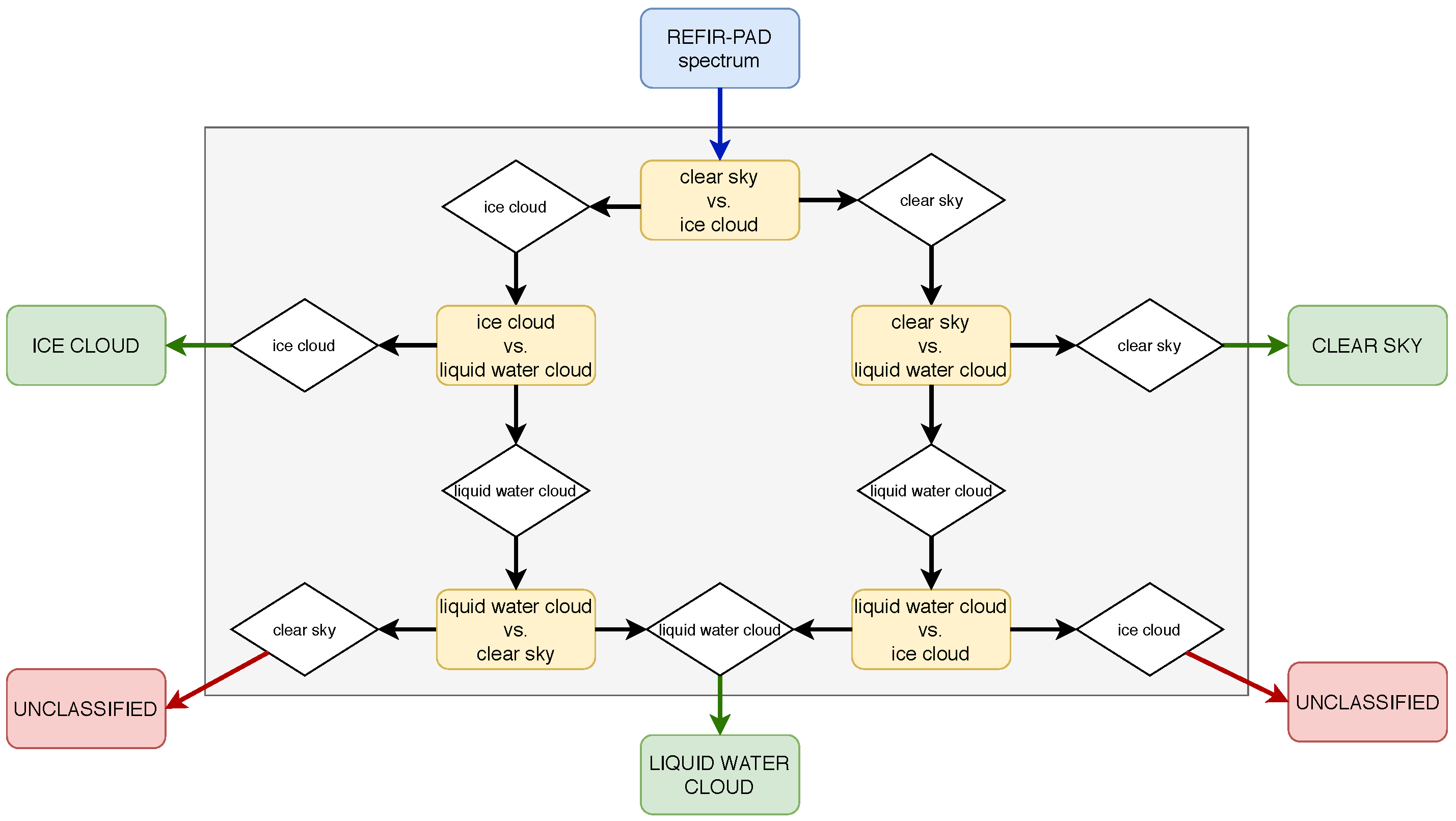
2.1. CIC: Cloud Identification and Classification
2.2. Polar Threshold, Cloud Base, and Top Height Retrieval
2.3. Simultaneous Atmospheric and Cloud Retrieval
3. Retrieval Setup
3.1. Selected Dataset of Spectral Radiances
3.2. Operational Choices
4. Results
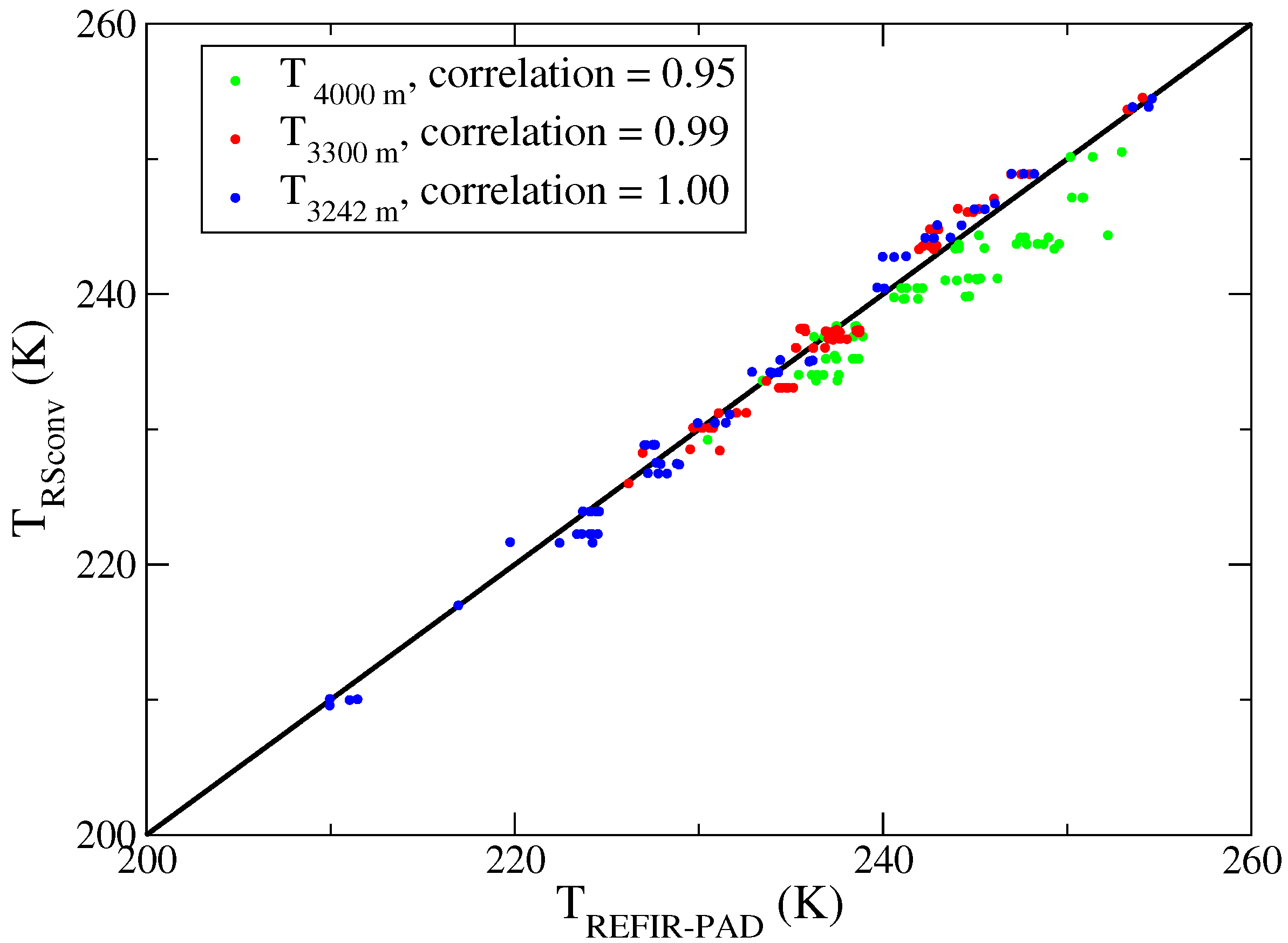
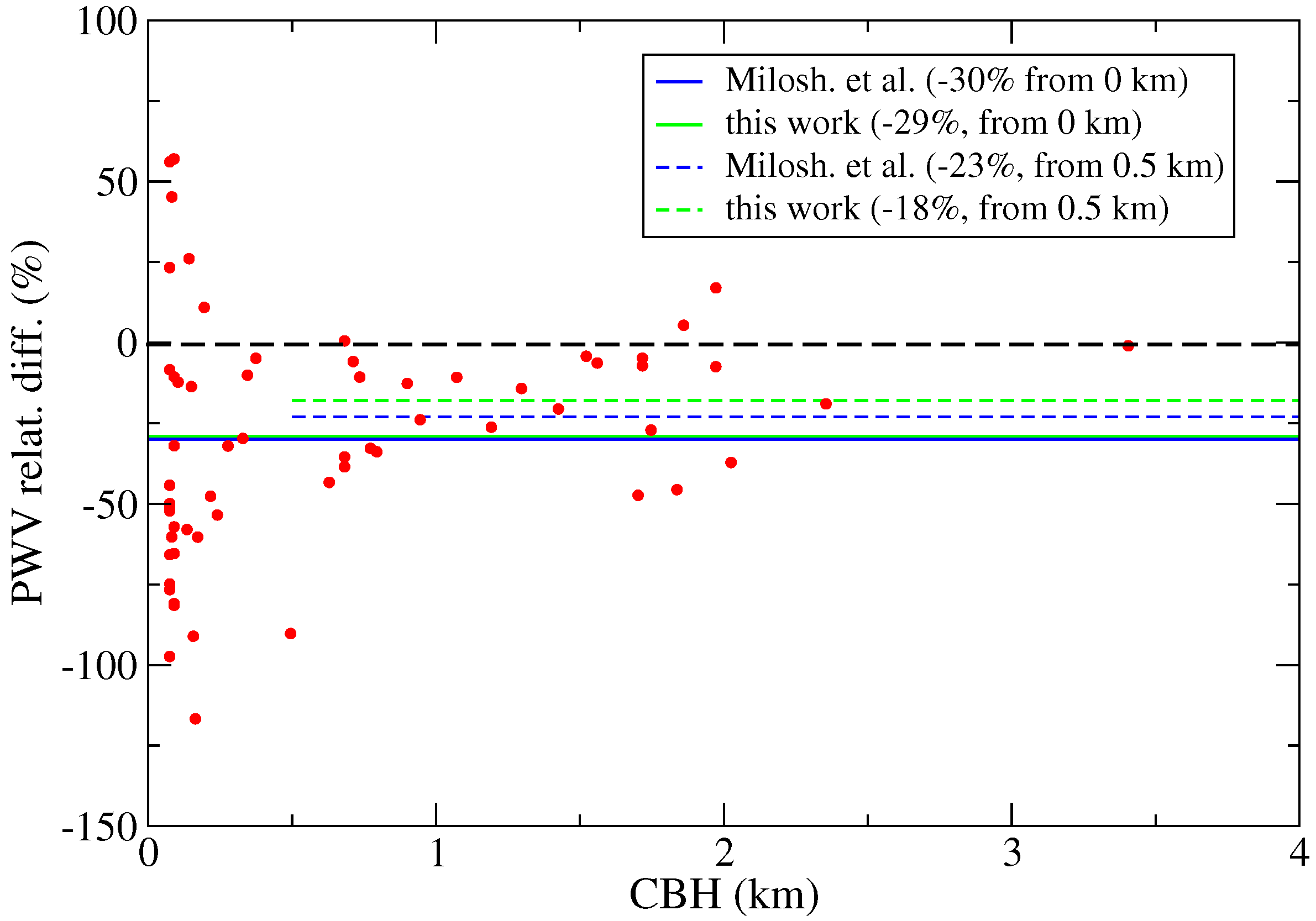
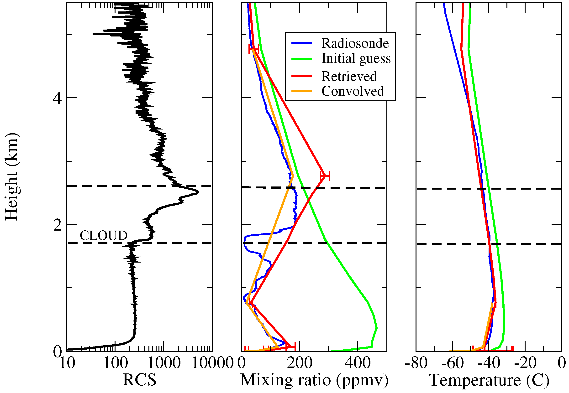
4.1. Validation of the Atmospheric Profiles
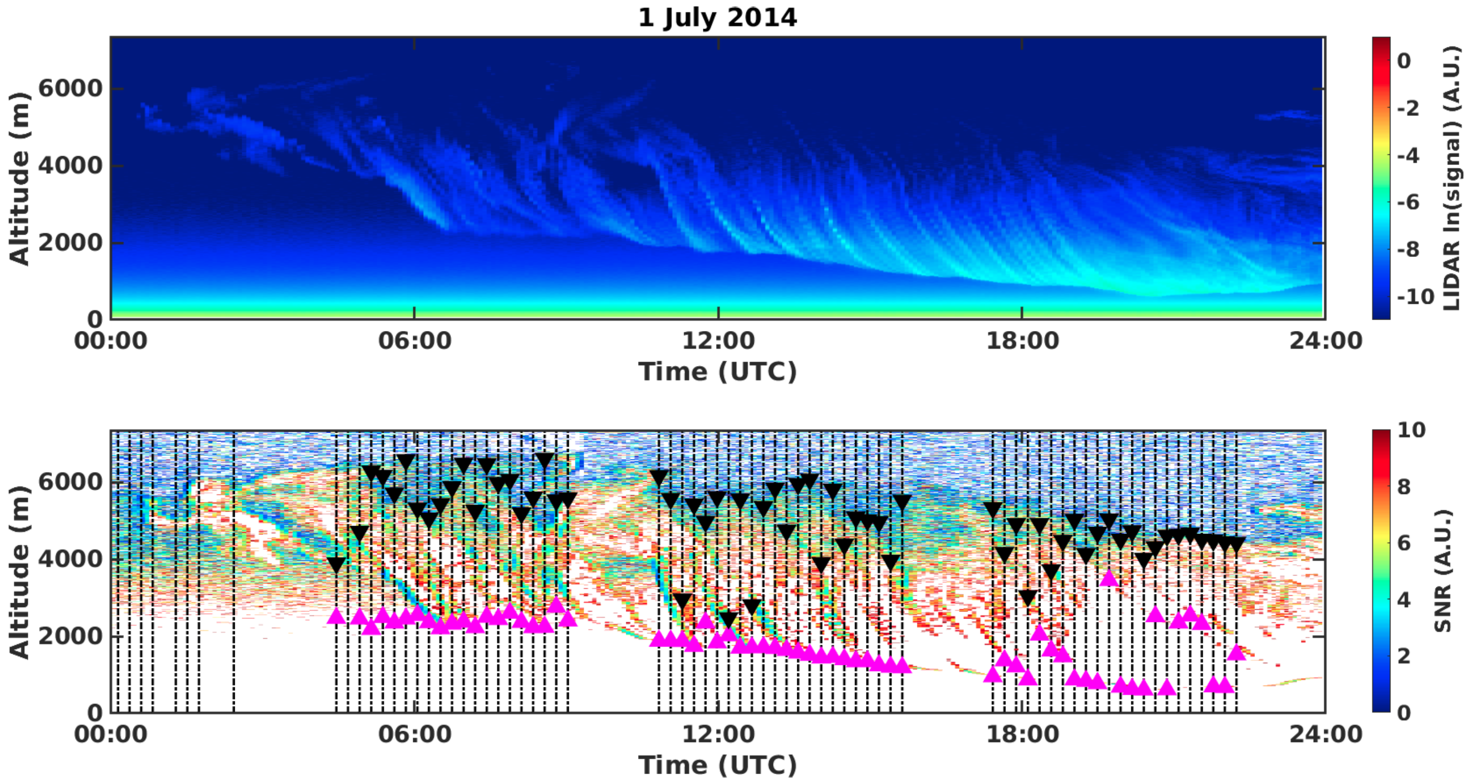
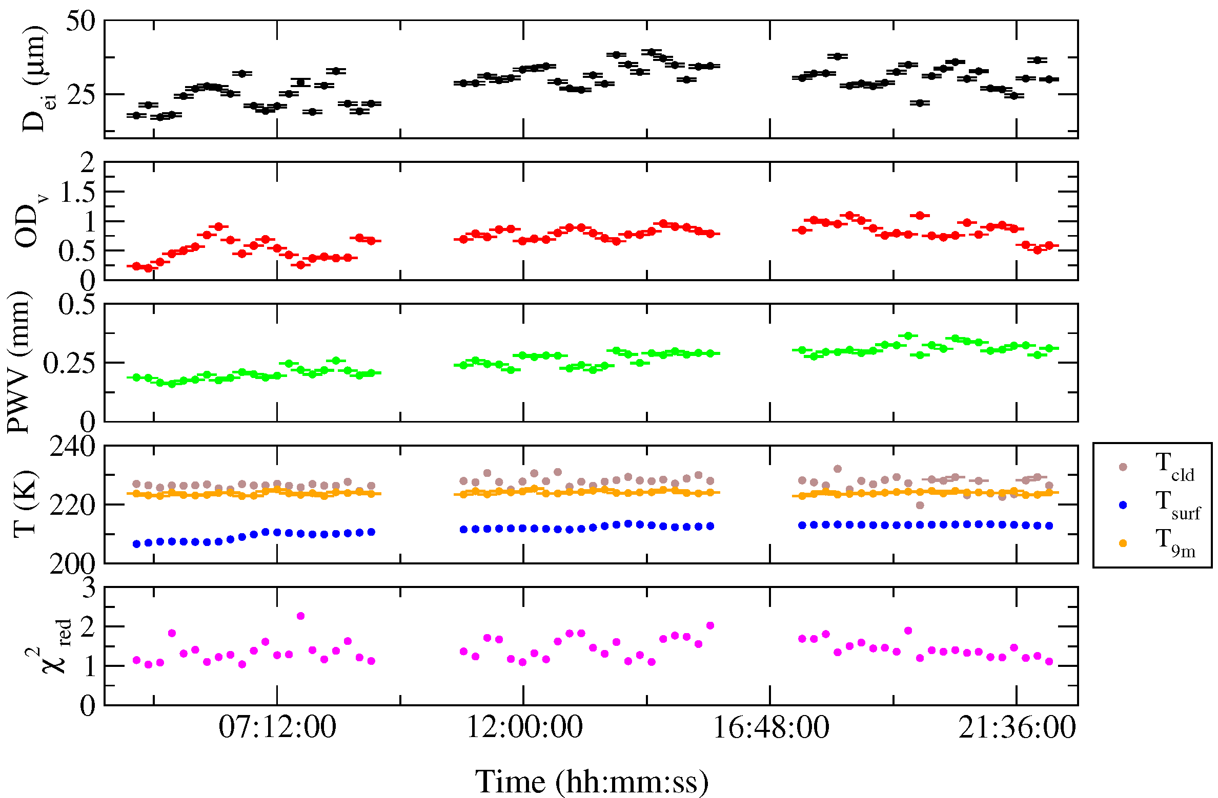
4.2. Case Study of 1 July 2014
4.3. Results from the Whole Dataset
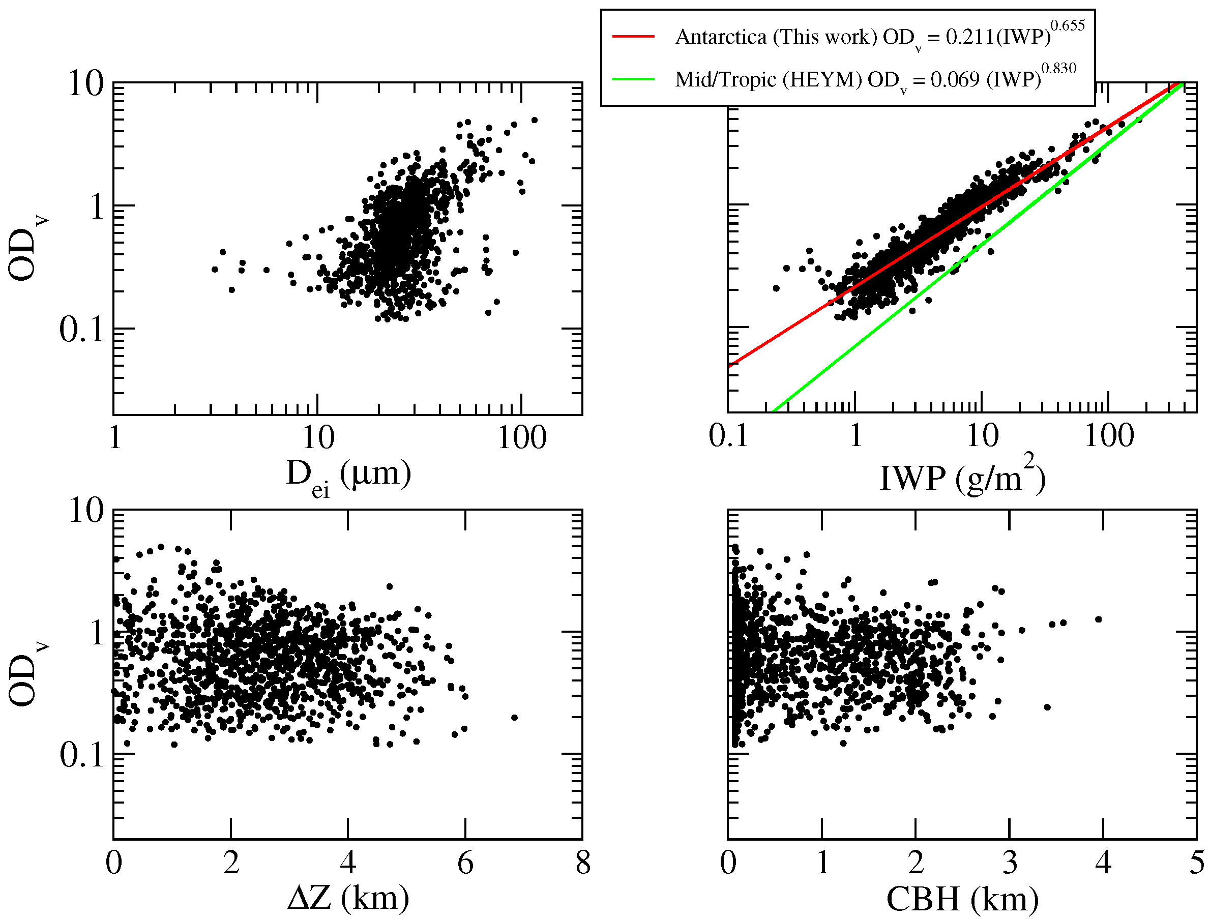
4.3.1. Ice Clouds
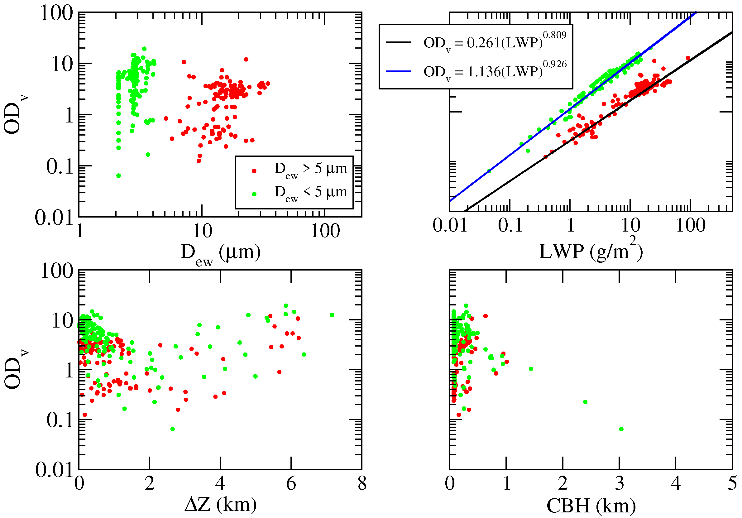
4.3.2. Water Clouds
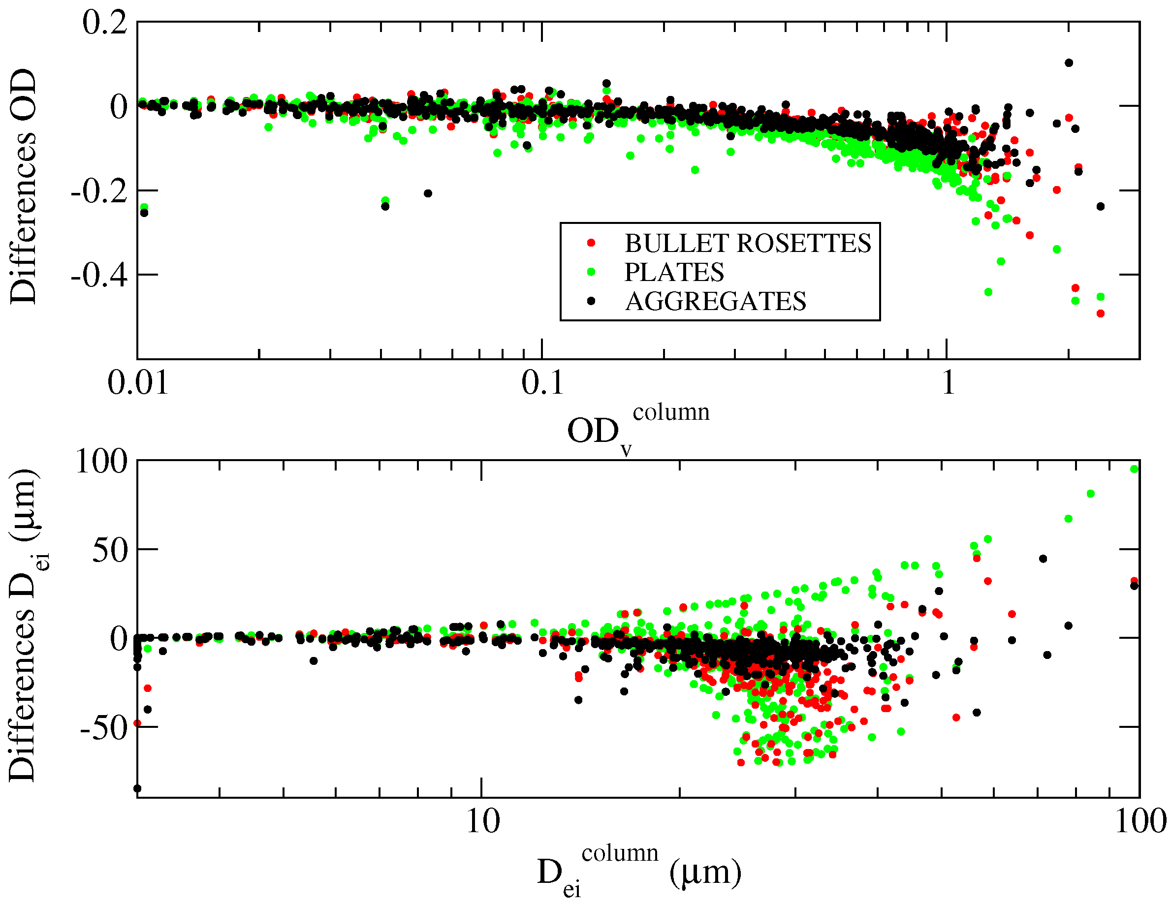
4.4. Sensitivity of Retrieved Parameters to the Crystal Habit
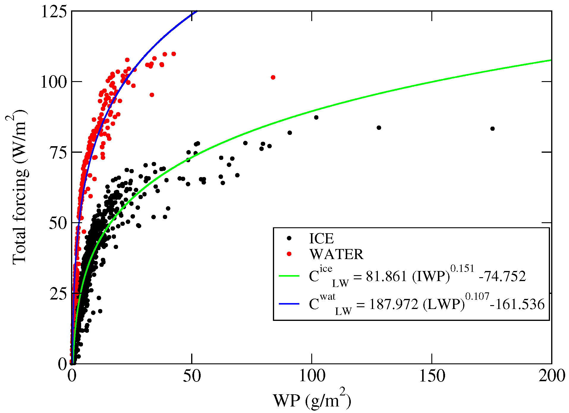
5. Assessment of Cloud Forcing
6. Summary of the Results
Author Contributions
Funding
Acknowledgments
Conflicts of Interest
References
- Cox, C.V.; Harries, J.E.; Taylor, J.P.; Green, P.D.; Baran, A.J.; Pickering, J.C.; Last, A.E.; Murray, J.E. Measurement and simulation of mid-and far-infrared spectra in the presence of cirrus. Q. J. R. Meteor. Soc. 2010, 136, 718–739. [Google Scholar] [CrossRef]
- Kiehl, J.T.; Trenberth, K.E. Earth’s annual global mean energy budget. Bull. Am. Meteorol. Soc. 1997, 78, 197–207. [Google Scholar] [CrossRef] [Green Version]
- Harries, J.; Carli, B.; Rizzi, R.; Serio, C.; Mlynczak, M.; Palchetti, L.; Maestri, T.; Brindley, H.; Masiello, G. The Far Infrared Earth. Rev. Geophys. 2008, 46. [Google Scholar] [CrossRef]
- Maesh, A.; Walden, V.P.; Warren, S.G. Ground-Based Infrared Remote Sensing of Cloud Properties over the Antarctic Plateau. Part I: Cloud-Base Heights. J. Appl. Meteorol. 2001, 40, 1265–1277. [Google Scholar] [CrossRef] [Green Version]
- Lubin, D.; Chen, B.; Bromwitch, D.H.; Somerville, R.C.J.; Lee, W.H.; Hines, K.M. The Impact of Antarctic Cloud Radiative Properties on a GCM Climate Simulation. J. Clim. 1998, 11, 447–462. [Google Scholar] [CrossRef] [Green Version]
- Palchetti, L.; Bianchini, G.; Di Natale, G.; Del Guasta, M. Far-Infrared radiative properties of water vapor and clouds in Antarctica. B. Am. Meteorol. Soc. 2015, 96, 1505–1518. [Google Scholar] [CrossRef]
- Maestri, T.; Cossich, W.; Sbrolli, I. Cloud identification and classification from high spectral resolution data in the far infrared and mid-infrared. Atmos. Meas. Tech. 2019, 12, 3521–3540. [Google Scholar] [CrossRef] [Green Version]
- Van Tricht, K.; Gorodetskaya, I.; Lhermitte, S.; Turner, D.; Schween, J.; Lipzig, N. An improved algorithm for cloud base detection by ceilometer over the ice sheets. Atmos. Meas. Tech. Discuss. 2013, 6, 9819–9855. [Google Scholar] [CrossRef]
- Di Natale, G.; Palchetti, L.; Bianchini, G.; Ridolfi, M. The two-stream δ-Eddington approximation to simulate the far infrared Earth spectrum for the simultaneous atmospheric and cloud retrieval. J. Quant. Spectrosc. Radiat. Transf. 2020, 246, 106927. [Google Scholar] [CrossRef]
- Di Natale, G.; Palchetti, L.; Bianchini, G.; Guasta, M.D. Simultaneous retrieval of water vapor, temperature and cirrus clouds properties from measurements of far infrared spectral radiance over the Antarctic Plateau. Atmos. Meas. Tech. 2017, 10, 825–837. [Google Scholar] [CrossRef] [Green Version]
- Clough, S.A.; Shephard, M.W.; Mlawer, E.J.; Delamere, J.S.; Iacono, M.J.; Cady-Pereira, K.; Boukabara, S.; Brown, P.D. Atmospheric radiative transfer modeling: A summary of the AER codes. J. Quant. Spectrosc. Radiat. Transf. 2005, 91, 233–244. [Google Scholar] [CrossRef]
- Mlawer, E.J.; Payne, V.H.; Moncet, J.L.; Delamere, J.S.; Alvarado, M.J.; Tobin, D.D. Development and recent evaluation of the MT_CKD model of continuum absorption. Phil. Trans. R. Soc. A 2012, 370, 2520–2556. [Google Scholar] [CrossRef] [PubMed] [Green Version]
- Yang, P.; Bi, L.; Baum, B.A.; Liou, K.N.; Kattawar, G.W.; Mishchenko, M.I.; Cole, B. Spectrally Consistent Scattering, Absorption, and Polarization Properties of Atmospheric Ice Crystals at Wavelengths from 0.2 to 100 μm. J. Atmos. Sci. 2013, 70, 330–347. [Google Scholar] [CrossRef]
- Rodgers, C.D. Inverse Methods for Atmospheric Sounding: Theory and Practice; World Scientific: Singapore, 2000. [Google Scholar] [CrossRef]
- Bianchini, G.; Castagnoli, F.; Di Natale, G.; Palchetti, L. A Fourier transform spectroradiometer for ground-based remote sensing of the atmospheric downwelling long-wave radiance. Atmos. Meas. Tech. 2019, 12, 619–635. [Google Scholar] [CrossRef] [Green Version]
- Palchetti, L.; Di Natale, G.; Bianchini, G. Remote sensing of cirrus microphysical properties using spectral measurements over the full range of their thermal emission. J. Geophys. Res. 2016, 121, 10–804. [Google Scholar] [CrossRef]
- Yang, P.; Wei, H.; Huang, H.; Baum, B.A.; Hu, Y.X.; Kattawar, G.W.; Mishchenko, M.I.; Fu, Q. Scattering and absorption property database for nonspherical ice particles in the near-through far-infrared spectral region. Appl. Opt. 2005, 44, 5512–5523. [Google Scholar] [CrossRef] [Green Version]
- Yang, P.; Mlynczak, M.G.; Wei, H.; Kratz, D.P.; Baum, B.A.; Hu, Y.X.; Wiscombe, W.J.; Heidinger, A.; Mishchenko, M.I. Spectral signature of ice clouds in the far-infrared region: Single-scattering calculations and radiative sensitivity study. J. Gophysical Res. 2003, 108, 1–15. [Google Scholar] [CrossRef]
- Kobayashi, T. Vapour growth of ice crystal between −40 and −90 °C. J. Meteorol. Soc. Jpn. 1965, 43, 359–367. [Google Scholar] [CrossRef] [Green Version]
- Shimizu, H. “Long prism” crystals observed in the precipitation in Antarctica. J. Meteorol. Soc. Jpn. 1963, 41, 305–307. [Google Scholar] [CrossRef] [Green Version]
- Lawson, R.P.; Baker, B.A.; Zmarzly, P.; O’Connor, D.; Mo, Q.; Gayet, J.F.; Shcherbakov, V. Microphysical and Optical Properties of Atmospheric Ice Crystals at South Pole Station. J. Appl. Meteorol. Climatol. 2006, 45, 1505–1524. [Google Scholar] [CrossRef]
- Turner, D.D. Arctic mixed-Phase cloud properties from AERI LiDAR observation: Algorithm and results from SHEBA. J. Appl. Meteorol. 2005, 44, 427–444. [Google Scholar] [CrossRef]
- Wiser, K.; Yang, P. Average ice crystal size and bulk short-wave single-scattering properties of cirrus clouds. Atmos. Res. 1998, 49, 315–335. [Google Scholar] [CrossRef]
- Remedios, J.J.; Leigh, R.J.; Waterfall, A.M.; Moore, D.P.; Sembhi, H.; Parkes, I.; Greenhough, J.; Chipperfield, M.P.; Hauglustaine, D. MIPAS reference atmospheres and comparisons to V4.61/V4.62 MIPAS level 2 geophysical data sets. Atmos. Chem. Phys. Discuss. 2007, 7, 9973–10017. [Google Scholar] [CrossRef] [Green Version]
- Stone, R.S. Properties of austral winter clouds derived from radiometric profiles at the South Pole. J. Geophys. Res. Atmos. 1993, 98, 12961–12971. [Google Scholar] [CrossRef]
- Maesh, A.; Walden, V.P.; Warren, S.G. Ground-based remote sensing of cloud properties over the Antarctic Plateau: Part II: Cloud optical depth and particle sizes. J. Appl. Meteorol. 2001, 40, 1279–1294. [Google Scholar] [CrossRef] [Green Version]
- Saxena, V.K.; Ruggiero, R.H. Antarctic Coastal Stratus Clouds: Microstructure and Acidity. In Contributions to Antarctic Research I; American Geophysical Union (AGU): Washington, DC, USA, 2013; pp. 7–18. [Google Scholar] [CrossRef]
- O’Shea, S.J.; Choularton, T.W.; Flynn, M.; Bower, K.N.; Gallagher, M.; Crosier, J.; Williams, P.; Crawford, I.; Fleming, Z.L.; Listowski, C.; et al. In situ measurements of cloud microphysics and aerosol over coastal Antarctica during the MAC campaign. Atmos. Chem. Phys. 2017, 17, 13049–13070. [Google Scholar] [CrossRef] [Green Version]
- Cady-Pereira, K.E.; Shephard, M.W.; Turner, D.D.; Mlawer, E.J.; Clough, S.A.; Wagner, T.J. Improved Daytime Column-Integrated Precipitable Water Vapor from Vaisala Radiosonde Humidity Sensors. J. Atmos. Ocean. Technol. 2008, 25, 873–883. [Google Scholar] [CrossRef]
- Dzambo, A.M.; Turner, D.D.; Mlawer, E.J. Evaluation of two Vaisala RS92 radiosonde solar radiative dry bias correction algorithms. Atmos. Meas. Tech. 2016, 9, 1613–1626. [Google Scholar] [CrossRef] [Green Version]
- Rizzi, R.; Maestri, T.; Arosio, C. Estimate of Radiosonde Dry Bias From Far-Infrared Measurements on the Antarctic Plateau. J. Geophys. Res. Atmos. 2018, 123, 3205–3211. [Google Scholar] [CrossRef]
- Miloshevich, L.M.; Vömel, H.; Paukkunen, A.; Heymsfield, A.J.; Oltmans, S.J. Characterization and Correction of Relative Humidity Measurements from Vaisala RS80-A Radiosondes at Cold Temperatures. J. Atmos. Ocean. Technol. 2001, 18, 135–156. [Google Scholar] [CrossRef]
- Heymsfield, A.J.; Matrosov, S.; Baum, B. Ice Water Path–Optical Depth Relationships for Cirrus and Deep Stratiform Ice Cloud Layers. J. Appl. Meteorol. 2003, 42, 1369–1390. [Google Scholar] [CrossRef]
- Lubin, D.; Harper, D.A. Cloud Radiative Properties over the South Pole from AVHRR Infrared Data. J. Clim. 1996, 9, 3405–3418. [Google Scholar] [CrossRef]
- Maestri, T.; Arosio, C.; Rizzi, R.; Palchetti, L.; Bianchini, G.; Del Guasta, M. Antarctic Ice Cloud Identification and Properties Using Downwelling Spectral Radiance From 100 to 1400 cm-1. J. Geophys. Res. Atmos. 2019, 124, 4761–4781. [Google Scholar] [CrossRef]
- Lachlan-Cope, T.; Ladkin, R.; Turner, J.; Davison, P. Observations of cloud and precipitation particles on the Avery Plateau, Antarctic Peninsula. Antarct. Sci. 2001, 13, 339–348. [Google Scholar] [CrossRef]
- Helt, J.E. Effects of Supersaturation and Temperature on Nucleation and Crystal Growth in a MSMPR Crystallizer. Ph.D. Thesis, Iowa State University Capstones, Ames, IA, USA, 1976; pp. 1–115. [Google Scholar]
- Town, M.S.; Walden, V.P.; Warren, S.G. Spectral and Broadband Longwave Downwelling Radiative Fluxes, Cloud Radiative Forcing, and Fractional Cloud Cover over the South Pole. J. Clim. 2005, 18, 4235–4252. [Google Scholar] [CrossRef]
- Intrieri, J.M.; Fairall, C.W.; Shupe, M.D.; Persson, P.O.G.; Andreas, E.L.; Guest, P.S.; Moritz, R.E. An annual cycle of Arctic surface cloud forcing at SHEBA. J. Geophys. Res. Ocean. 2002, 107, SHE 13-1–SHE 13-14. [Google Scholar] [CrossRef]
- Clough, S.A.; Iacono, M.J.; Moncet, J.L. Line-by-line calculations of atmospheric fluxes and cooling rates: Application to water vapor. J. Geophys. Res. Atmos. 1992, 97, 15761–15785. [Google Scholar] [CrossRef]
- Pavolonis, M.J.; Key, J.R. Antarctic Cloud Radiative Forcing at the Surface Estimated from the AVHRR Polar Pathfinder and ISCCP D1 Datasets, 1985–93. J. Appl. Meteorol. 2003, 42, 827–840. [Google Scholar] [CrossRef]
- Allan, R.P. Evaluation of Simulated Clear-Sky Longwave Radiation Using Ground-Based Observations. J. Clim. 2000, 13, 1951–1964. [Google Scholar] [CrossRef] [Green Version]
- Stone, R.; Dutton, E.; DeLuisi, J. Surface radiation and temperature variations associated with cloudiness at the South Pole. Antarct. J. 1989, 24, 230–232. [Google Scholar]
- Dutton, E.G.; Stone, R.S.; Nelson, D.W.; Mendonca, B.G. Recent Interannual Variations in Solar Radiation, Cloudiness, and Surface Temperature at the South Pole. J. Clim. 1991, 4, 848–858. [Google Scholar] [CrossRef]
- Palchetti, L.; Brindley, H.; Bantges, R.; Buehler, S.A.; Camy-Peyret, C.; Carli, B.; Cortesi, U.; Del Bianco, S.; Di Natale, G.; Dinelli, B.M.; et al. FORUM: Unique far-infrared satellite observations to better understand how Earth radiates energy to space. Bull. Am. Meteorol. Soc. 2020, 1–52. [Google Scholar] [CrossRef]


| Instrument | Measure | Exploited Spectral Band | Retrieved Parameters | Algorithm |
|---|---|---|---|---|
| REFIR-PAD | spectral radiance | 200–980 cm | , OD, HO/T profiles | SACR |
| REFIR-PAD | spectral radiance | 380–1000 cm | phase (ice or liquid) | CIC |
| LiDAR | Backscatt./depolar. signal | 532 nm | CBH, CTH | PT |
| Authors | Location | (m) | Crystals Type |
|---|---|---|---|
| This work | Concordia (2013–2014), 1439 spectra | 28 | Columns |
| 55 | Plates | ||
| 51 | Bullet rosettes | ||
| 35 | Aggregates | ||
| Lawson et al. (2006) | South Pole (February 2001) | 21 () * | Columns |
| 38 () * | Plates | ||
| 54 () * | Bullet rosettes | ||
| Walden et al. (2003) | South Pole (winter 1992) | 20 | Columns |
| 30 | Plates | ||
| 50 | Bullet cluster | ||
| Mahesh et al. (2001) | South Pole (1992) | 30 | |
| Stone (1993) | South Pole (1959–1963) | 8–32 | All crystals |
| Lubin and Harper (1996) | South Pole (summer, 1992) | 25 | |
| South Pole (winter, 1992) | 11 | ||
| Maestri et al. (2019) | Concordia (2013), 26 selected spectra | 50 | Columns |
| 40 | Plates | ||
| 38 | Bullet rosettes | ||
| 50 | Aggregates | ||
| Shimizu (1963) | Byrd Station (winter, 1961) | 100–1000 (length) | Long columns |
| Lachlan-Cope et al. (2001) | Avery Plateau (1995) | 20–200 | All crystals |
| Authors | Location | Lat, Lon | Alt (m a.s.l.) | Forcing (W/m) |
|---|---|---|---|---|
| This work | Concordia (2013–2014) | 75S, 123E | 3233 | 30 (ice clouds only) |
| This work | Concordia (2013–2014) | 75S, 123E | 3233 | 46 (ice + water clouds) |
| Town et al. (2005) | South Pole (2001) | 90S | 2835 | 20 |
| South Pole (1992) | 90S | 2835 | 24 | |
| Pavolonis and Key (2003) | Antarctic cont.(1985–1993) | 75S | ∼30 | |
| Intrieri et al. (2002) | SHEBA (Nov.1997– Oct.1998) | 77N, 165W | 0 | 38 |
| Allan (2000) | Barrow, Alaska (1992) | 71.3N, 156.6W | 0 | 44 |
Publisher’s Note: MDPI stays neutral with regard to jurisdictional claims in published maps and institutional affiliations. |
© 2020 by the authors. Licensee MDPI, Basel, Switzerland. This article is an open access article distributed under the terms and conditions of the Creative Commons Attribution (CC BY) license (http://creativecommons.org/licenses/by/4.0/).
Share and Cite
Di Natale, G.; Bianchini, G.; Del Guasta, M.; Ridolfi, M.; Maestri, T.; Cossich, W.; Magurno, D.; Palchetti, L. Characterization of the Far Infrared Properties and Radiative Forcing of Antarctic Ice and Water Clouds Exploiting the Spectrometer-LiDAR Synergy. Remote Sens. 2020, 12, 3574. https://doi.org/10.3390/rs12213574
Di Natale G, Bianchini G, Del Guasta M, Ridolfi M, Maestri T, Cossich W, Magurno D, Palchetti L. Characterization of the Far Infrared Properties and Radiative Forcing of Antarctic Ice and Water Clouds Exploiting the Spectrometer-LiDAR Synergy. Remote Sensing. 2020; 12(21):3574. https://doi.org/10.3390/rs12213574
Chicago/Turabian StyleDi Natale, Gianluca, Giovanni Bianchini, Massimo Del Guasta, Marco Ridolfi, Tiziano Maestri, William Cossich, Davide Magurno, and Luca Palchetti. 2020. "Characterization of the Far Infrared Properties and Radiative Forcing of Antarctic Ice and Water Clouds Exploiting the Spectrometer-LiDAR Synergy" Remote Sensing 12, no. 21: 3574. https://doi.org/10.3390/rs12213574