Article

Consistent Comparison of Remotely Sensed Sea Ice Concentration Products with ERA-Interim Reanalysis Data in Polar Regions

1
Key Laboratory of Digital Earth Science, Aerospace Information Research Institute, Chinese Academy of Sciences, Beijing 100094, China
2
University of Chinese Academy of Sciences, Beijing 100049, China
3
State Key Laboratory of Remote Sensing Science, Aerospace Information Research Institute, Chinese Academy of Sciences, Beijing 100101, China
4
College of Surveying and Geo-Informatics, North China University of Water Resources and Electric Power, Zhengzhou 450045, China
5
State Key Laboratory of Earthquake Dynamics, Institute of Geology, China Earthquake Administration, Beijing 100029, China
*
Author to whom correspondence should be addressed.
Remote Sens. 2020, 12(18), 2880; https://doi.org/10.3390/rs12182880
Submission received: 22 June 2020 / Revised: 17 August 2020 / Accepted: 31 August 2020 / Published: 5 September 2020
(This article belongs to the Special Issue Recent Advances in Cryospheric Sciences)

Abstract

:
Sea ice concentration (SIC) plays a significant role in climate change research and ship’s navigation in polar regions. Satellite-based SIC products have become increasingly abundant in recent years; however, the uncertainty of these products still exists and needs to be further investigated. To comprehensively evaluate the consistency of the SIC derived from different SIC algorithms in long time series and the whole polar regions, we compared four passive microwave (PM) satellite SIC products with the ERA-Interim sea ice fraction dataset during the period of 2015–2018. The PM SIC products include the SSMIS/ASI, AMSR2/BT, the Chinese FY3B/NT2, and FY3C/NT2. The results show that the remotely sensed SIC products derived from different SIC algorithms are generally in good consistency. The spatial and temporal distribution of discrepancy among satellite SIC products for both Arctic and Antarctic regions are also observed. The most noticeable difference for all the four SIC products mostly occurs in summer and at the marginal ice zone, indicating that large uncertainties exist in satellite SIC products in such period and areas. The SSMIS/ASI and AMSR2/BT show relatively better consistency with ERA-Interim in the Arctic and Antarctic, respectively, but they exhibit opposite bias (dry/wet) relative to the ERA-Interim data. The sea ice extent (SIE) and sea ice area (SIA) derived from PM and ERA-Interim SIC were also compared. It is found that the difference of PM SIE and SIA varies seasonally, which is in line with that of PM SIC, and the discrepancy between PM and ERA-Interim data is larger in Arctic than in Antarctic. We also noticed that different algorithms have different performances in different regions and periods; therefore, the hybrid of multiple algorithms is a promising way to improve the accuracy of SIC retrievals. It is expected that our findings can contribute to improving the satellite SIC algorithms and thus promote the application of these useful products in global climate change studies.

1. Introduction

Sea ice concentration (SIC) is defined as the percentage of the area occupied by sea ice, which is a common parameter used in climate models [1,2], and it also plays a vital role in ship navigation [3,4]. Long-term and large-scale SIC data of polar regions are essential for climate change studies, especially with the recent decline of Arctic sea ice and increase of Antarctic sea ice [5,6,7,8,9].
Passive microwave (PM) remote sensing has been proved to be an effective way to observe sea ice in polar regions both temporally and spatially, mainly due to its high sensitivity to dielectric properties of sea ice and its capability of all-time and all-weather coverage. Over the last few decades, considerable efforts have been devoted to developing various SIC retrieval algorithms from PM observations, but only some of them, e.g., the NASA Team (NT) [10], enhanced NT (NT2) [11], NASA Bootstrap (BT) [12], Arctic Radiation and Turbulence Interaction Study Sea Ice (ASI) [13,14], and Ocean and Sea ice Satellite Application Facility (OSI-SAF) sea ice algorithms [15,16], are used to operationally generate SIC products. To date, various satellite PM sensors, such as Scanning Multichannel Microwave Radiometer (SMMR), Special Sensor Microwave Imager/Sounder (SSMI/SSMIS), Advanced Microwave Scanning Radiometer for Earth Observing System (AMSR-E), and its successor AMSR2, as well as the Chinese Feng Yun-3 (FY3) Microwave Radiation Imager (MWRI), have routinely provided SIC products to the public free of charge. Although satellite-based SIC products have become increasingly abundant in recent years, they can only be applied in practical applications after being fully validated. A good knowledge of the quality of the satellite SIC products is of great importance for their application and improvement, and can not only help users to better select suitable products for their research, but also help algorithm developers for further algorithm refinements. Thus, it is necessary and essential to examine the uncertainties and limitations of various remotely sensed SIC products in polar regions.
A number of validation activities have been conducted for the PM SIC products in recent years. Ivanova et al. [17] presented some key results of an extensive algorithm inter-comparison and evaluation experiment. Meier et al. [18] compared the SIC from operational data with PM estimates and assessed the uncertainties in sea ice extent climate indicators [19]. Wiebe et al. [20] examined the accuracy of AMSR-E ASI products by using Landsat-7 ETM+ and synthetic aperture radar (SAR) images during the Arctic spring. Cavalieri et al. [21] assessed the AMSR-E Antarctic winter SIC using Aqua Moderate Resolution Imaging Spectroradiometer (MODIS) data. Several researches investigated the skill of satellite SIC by using ship observations from Chinese National Arctic Research Expedition (CHINARE) [22,23] or Antarctic Sea Ice Processes and Climate (ASPeCt) [24,25,26]. Though many studies have been conducted to validate the PM SIC products using optical data, SAR images, ship observation records, or their combination [4,21,27,28,29,30,31,32,33,34,35], these methods have some limitations in both space and time [19]. For example, the optical data are vulnerable to weather conditions, such as cloud cover, which is particularly prominent in polar regions. The SAR data may suffer from the ambiguity issue in SIC classification, though they are all-weather, daylight independent, and fine-resolution data. Ship observations are usually treated as “ground truth” as they are the only ground SIC observations; however, they are usually biased towards thin, easy to navigate sea ice and cover a comparably small region. Moreover, these validation activities were conducted only over a short time period in a few locations, and therefore the results may be regionally dependent and sometimes even lead to inconsistent conclusions. The reanalysis dataset, which has a comparable spatial and temporal resolution as the PM SIC products, provides an opportunity to evaluate the consistency between PM and reanalysis SIC dataset. This can help us understand the spatial and temporal distribution of discrepancy in the SIC products in the whole polar regions for a long time series. Furthermore, to our knowledge, there is little information available in the literature about the quality of the new Chinese FY3 SIC products in the whole polar regions. Therefore, it is imperative to assess the FY3 SIC products to get more useful feedback for further improvement of the product quality. Even though the reanalysis dataset cannot be regarded as the true SIC, it is a valuable source of reference information. The comparison will be useful to detect the inconsistency and assess the consistency between the two kinds of SIC products and find possible errors in the PM SIC products for further algorithm improvement.
In this study, we provide the assessment of four PM SIC products, including the DMSP SSMIS with ASI algorithm (SSMIS/ASI), the GCOM-W AMSR2 with BT algorithm (AMSR2/BT), the new Chinese Feng Yun-3B with enhanced NT2 algorithm (FY3B/NT2), and the Chinese Feng Yun-3C with NT2 algorithm (FY3C/NT2) in whole Arctic and Antarctic regions by adopting a reanalysis SIC, namely, the ERA-Interim sea ice fraction data (ERA SIC) as the reference to evaluate the consistency between PM SIC and ERA SIC. This paper aims to improve the understanding of the similarities and differences of different SIC datasets, which not only can guide the users to take maximum advantage of these valuable data, but also can identify the possible error sources for future algorithm refinements. The paper is organized as follows. The data used in the study are briefly introduced in Section 2. Section 3 describes the data processing and evaluation method. Then, the detailed comparison of the PM SIC with respect to ERA SIC is presented in Section 4. Finally, the discussion and concluding remarks are given in Section 5 and Section 6, respectively.

2. Materials

Due to a lack of long-time series of sea ice measurements at satellite footprint scale, it is challenging to assess the consistency of PM SIC products. Compared with traditional optical and SAR images, or ship-based records, the sea ice fraction dataset from ERA-Interim can be used as reference data for a polar-wide and long-time series comparison with other PM SIC data. A brief description of the SIC products are presented in the following Table 1.
The SSMIS boarded on DMSP has been used to monitor SIC for almost forty years. The SIC values estimated by using the ASI algorithm from SSMIS brightness temperatures at 91 GHz were used in this study. The ASI algorithm was originated from the Arctic Radiation and Turbulence Interaction Study Project in 1998. It improves the SIC algorithm by using 90 GHz brightness temperature from SMMR proposed by Svendsen et al. [36]. Compared with other algorithms which used 85/89/90/91 GHz, it has the advantage of no extra data to introduce but with the same performance as other high-frequency algorithms. In order to reduce the weather influence, a 5-day median filter was applied in the product [37]. More details of the ASI algorithm can be found in [13,14]. The SSMIS/ASI SIC product used in this study is provided from 1991 onwards with a grid resolution of 12.5 km [13]. It is freely provided by the University of Hamburg and can be downloaded (http://icdc.cen.uni-hamburg.de).
The AMSR2 sensor has been operating aboard the JAXA GCOM-W1 satellite from 2012 onwards. It is the successor of AMSR-E boarded on the NASA Aqua satellite. It provides data on both horizontal and vertical polarized brightness temperatures at six different frequencies in the range between 6.9 and 89.0 GHz. In this study, the AMSR2 SIC products retrieved by using the BT algorithm were adopted. The BT algorithm, which is developed by Comiso [12], uses brightness temperature at both 37 GHz and 19 GHz to retrieve SIC. A detailed description of the BT algorithm can be found in [12]. The AMSR2/BT SIC product used in this study is provided by the University of Bremen. However, it should be mentioned that the University of Bremen does not deliver AMSR2/BT SIC product nowadays. Other sources for BT algorithm are the AMSR2/BT product provided by the Japan Aerospace Exploration Agency (JAXA) (https://gportal.jaxa.jp/gpr/) and the SSMIS/BT product provided by the National Snow and Ice Data Center (NSIDC) (https://nsidc.org/data/nsidc-0079).
The Chinese FY3B and FY3C satellites were launched in 2010 and 2013, respectively. The microwave sensor loaded on the FY3B and FY3C satellites is the MWRI, which provides observations with frequencies ranging from 10.7 to 89.0 GHz. The only main difference of FY3B and FY3C is that their overpass time is different. The FY3B scans the Earth’s surface in an ascending (1:40 P.M. local solar time) and descending (1:40 A.M. local solar time) mode, while the local equatorial overpass time of the FY3C is 10:15 P.M. (ascending) and 10:15 A.M. (descending). Both FY3B and FY3C adopted the NT2 algorithm to generate SIC products. The NT2 algorithm improves the atmosphere radiation characteristics based on the NT algorithm by using the polarization gradient ratio and the polarization rotation gradient ratio. An optimization algorithm that includes a look-up table for brightness temperatures calculated for various atmospheric conditions is used in the NT2 algorithm. More details of the NT2 algorithm can be found in [11]. The FY3B/NT2 and FY3C/NT2 SIC products (namely, FY3 SIC) include daily ascending averages, daily descending averages, and daily averages, which are produced by the Chinese National Satellite Meteorological Centre (CNSMC) since 2011 and 2014, respectively. The daily SIC averages with a grid resolution of 12.5 km were used for comparison with other two SIC products and ERA SIC. The FY3B and FY3C SIC products can be freely obtained from CNSMC after registration (http://satellite.nsmc.org.cn).
ERA-Interim is a reanalysis of the global atmosphere produced by the European Centre for Medium-Range Weather Forecasts (ECMWF), which covers the data-rich period since 1979 and continues in real-time [38]. Sea ice area fraction, the fraction of a grid box which is covered by sea ice, is an analysis variable in ERA-Interim, which can be retrieved at latitude/longitude grid resolution of 0.125°–3°. The SIC dataset used in ECMWF for the period of 2015–2018 comes from the operational EUMETSAT OSI SAF SIC product [38], which is derived from SSMIS based on a smooth combination of BT and Bristol algorithms [39]. It should be noted that ERA-Interim does not incorporate its analysis of the SIC, but rather as boundary conditions for the atmospheric forecast model. At ECMWF, the SIC fields are resampled to the reduced Gaussian grid used in the Integrated Forecasting System (IFS). In the study, we used the ERA-Interim sea ice fraction data in the period of 2015 to 2018, and the grid resolution of ERA-Interim SIC is quarter-degree latitude by quarter-degree longitude grid (i.e., 0.125°) consistent with other SIC products. Moreover, compared to the original SIC data source, ERA has more additional processing, including coarse quality control bounds, weather filtering on the grid, a posteriori filtering, sea surface temperature filtering, and land mask, which potentially provide reliable mapping of the SIC.

3. Methods

For a consistent and fair comparison, the nearest interpolation method was adopted to resample ERA SIC to a grid resolution of 12.5 km to match with PM SIC grids [40]. Both monthly and annual SIC calculated from daily SIC during the period from 1 January 2015 to 31 December 2018 (a total of four years) were selected to compare and evaluate the consistency of the PM SIC products with respect to the ERA SIC product. For the monthly SIC data, the error metrics were calculated on a grid-by-grid basis by using all the data in every month (e.g., for January, all the data in January of each year from 2015 to 2018 were used). For the annual SIC data, the error metrics were calculated on a grid-by-grid basis by using all the data for the four years (e.g., for a specific grid, the data from 1 January 2015 to 31 December 2018 were used). The null data (e.g., the land) were not considered in the calculation. In our study, Arctic and Antarctic are individually evaluated using monthly and annual SIC. Moreover, the daily sea ice extent (SIE) and sea ice area (SIA) derived from PM and ERA SIC data are compared. The 15% threshold is usually used for both SIE and SIA calculations [41]. Specifically, SIA is defined as the sum of the product of pixel area and SIC for SIC greater than 15%, while SIE is simply the sum of all the pixel areas with SIC greater than 15% [42]. The 15% threshold was chosen because it on average corresponded with the true ice edge in validation studies when the algorithms were being developed [43]. As ERA-Interim SIC data is not considered as the “true” SIC values and may contain errors, we use the root mean square difference (RMSD) instead of root mean square error (RMSE) to characterize the discrepancy of the SIC products. Besides, we consider standard deviation ratio (σ), which can describe the product fluctuation. Four statistical indicators, including the mean bias (Bias), RMSD, σ, and the Spearman correlation coefficient (R), were computed to quantitatively evaluate the consistency between four PM SIC products and reanalysis dataset: RMSD is the representation of absolute difference between satellite data and reference data; the Bias represents the mean difference between satellite retrievals and reference data; R is a measure of the strength of an association between two variables and the Spearman correlation coefficient is able to describe a relationship between two variables without making any assumptions about the frequency distribution of the variables [44]; the standard deviation ratio represents the volatility of satellite SIC compared to the reference data. If σ > 1, it implies that the volatility of satellite SIC is larger than that of ERA SIC, and if σ < 1, it indicates the volatility of satellite SIC is smaller than that of ERA SIC.
R M S D = i = 1 n ( x i y i ) 2 n 1
B i a s = i = 1 n ( x i y i ) n
σ = σ P M σ E R A
R = 1 6 i = 1 n ( y i x i ) 2 n ( n 2 1 )
where x i and x ¯ represent PM remotely sensed SIC and its average, respectively. y i and y ¯ denote ERA SIC and its average, respectively. n is the total number of samples. σ P M and σ E R A are the standard deviation of PM SIC and ERA SIC, respectively, which can be explained the volatility and dynamic changes of products. The larger the value of σ, the greater the fluctuation of products.

4. Results

In this section, the statistical indicators of four PM SIC, SIE, and SIA concerning RMSD, Bias, σ, and R with regard to ERA SIC were computed in both Arctic and Antarctic. First, the spatial patterns of daily SIC were presented, which can illustrate the polar-scale consistency and discrepancy between four PM SIC and ERA SIC, shown in Figure 1 and Figure 2 for Arctic and Antarctic, respectively. Then, we examined the temporal behavior of monthly SIC during the study period, which can reveal how the temporal distribution characteristic of the discrepancy between PM SIC and ERA SIC products varies seasonally. The statistical metrics of the four average monthly PM SIC products are displayed in Figure 3 and Figure 4. Four error metrics (RMSD, Bias, σ, and R) used to quantify the consistency of the four SIC products were computed for average monthly SIC, which are summarized in Table 2. To further investigate the annual discrepancy of each satellite algorithm, we examined the spatial pattern of annual SIC to make a clearer view of the consistency between them, shown in Figure 5 for Arctic and Figure 6 for Antarctic. Moreover, Figure 7 and Figure 8 present the temporal evolution of daily SIE and its bias between four PM SIC and ERA SIC. Figure 9 and Figure 10 are similar to Figure 7 and Figure 8 but for daily SIA. Finally, the detailed statistical indicators of the daily SIE and SIA are described in Table 3 and Table 4 respectively.

4.1. Daily average SIC Calculated from PM SIC and ERA SIC

The daily average spatial pattern of four PM SIC and ERA SIC in the Arctic for the period of 2015–2018 is shown in Figure 1. Four remotely sensed SIC products exhibit a similar spatial distribution with ERA SIC, with a noticeable decrease from near polar center to sea ice marginal zone. In marginal ice zones (e.g., Bering Sea and Okhostsk Sea), the SIC is generally below 20%. The high SIC locates in the high latitudes, where the PM SIC is generally consistent with ERA SIC, though with some discrepancies. The SSMIS/ASI has the highest consistency with ERA SIC in general while AMSR2 SIC product exhibits more sea ice in the marginal ice zone. The spatial distribution of the FY3B/NT2 and FY3C/NT2 is highly consistent, which is in line with expectations, as they adopted the same algorithm to generate SIC products.
Figure 2 depicts the spatial pattern regarding the daily average PM and ERA SIC products in Antarctic. The spatial distribution of the four PM SIC products agree even better with ERA SIC in Antarctic than in Arctic. Similar to Arctic, the SIC values decrease as the latitude decreases in Antarctic. This is because high latitude regions (e.g., Weddell Sea) more commonly have higher multiyear ice fractions, resulting in higher SIC values. The AMSR2/BT, FY3B/NT2, and FY3C/NT2 are somewhat different from the SSMIS/ASI product when compared with ERA SIC in the location where SIC is above 90%. It can be seen that in these regions the SSMIS/ASI product shows lower SIC values, whereas the others present marginally higher SIC values. In the Ross Sea, the FY3B/NT2 and FY3C/NT2 overestimate the ERA SIC than the AMSR2/BT. Meanwhile, the SSMIS/ASI slightly underestimate the ERA SIC. In general, the AMSR2/BT product seems in best agreement with ERA SIC in Antarctic visually.

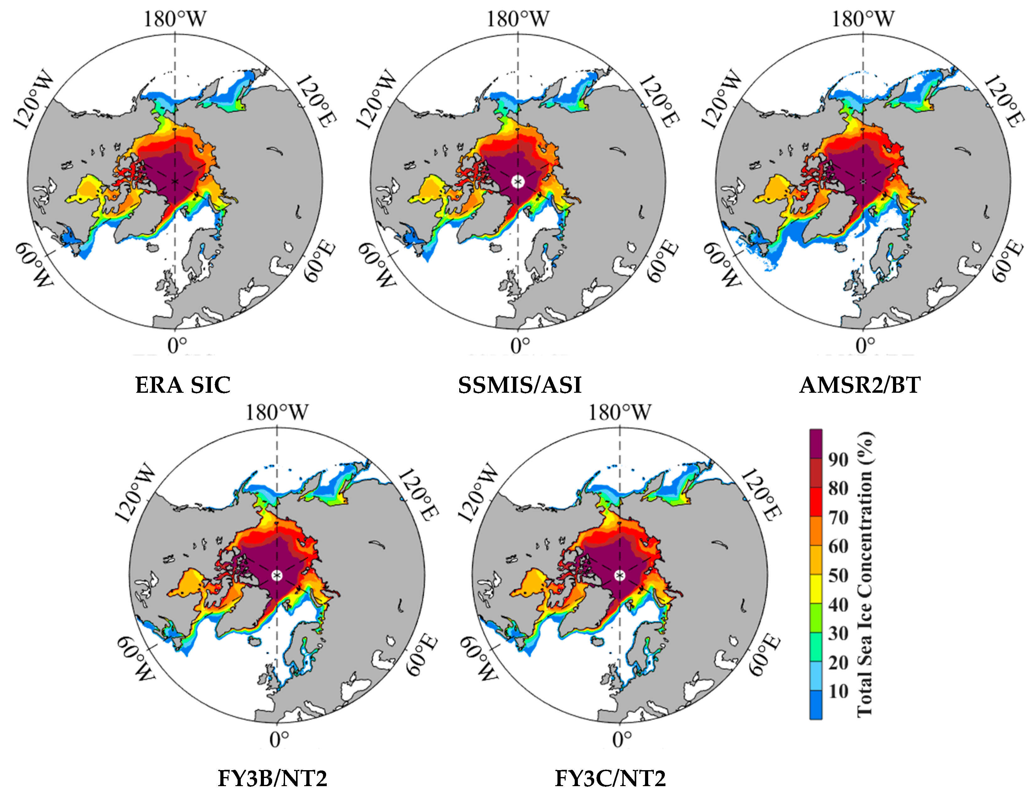
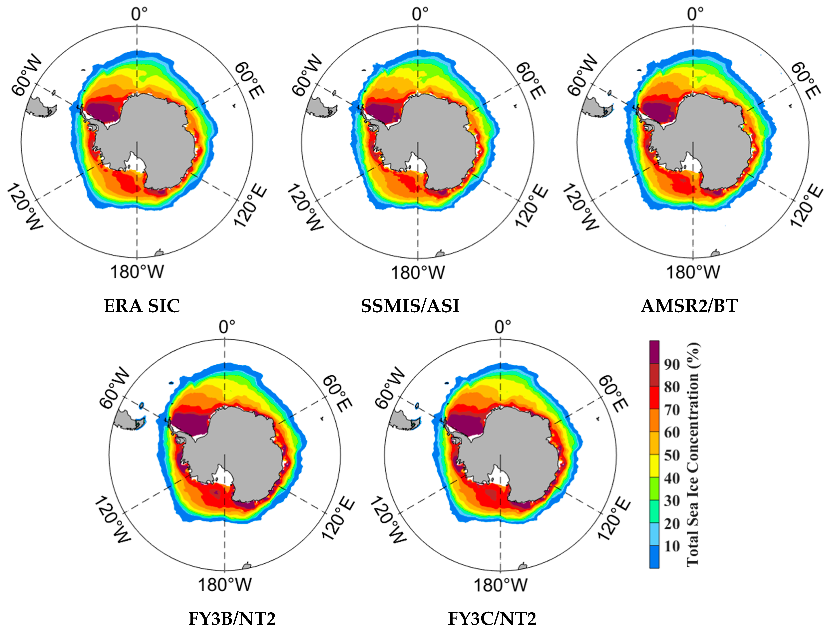
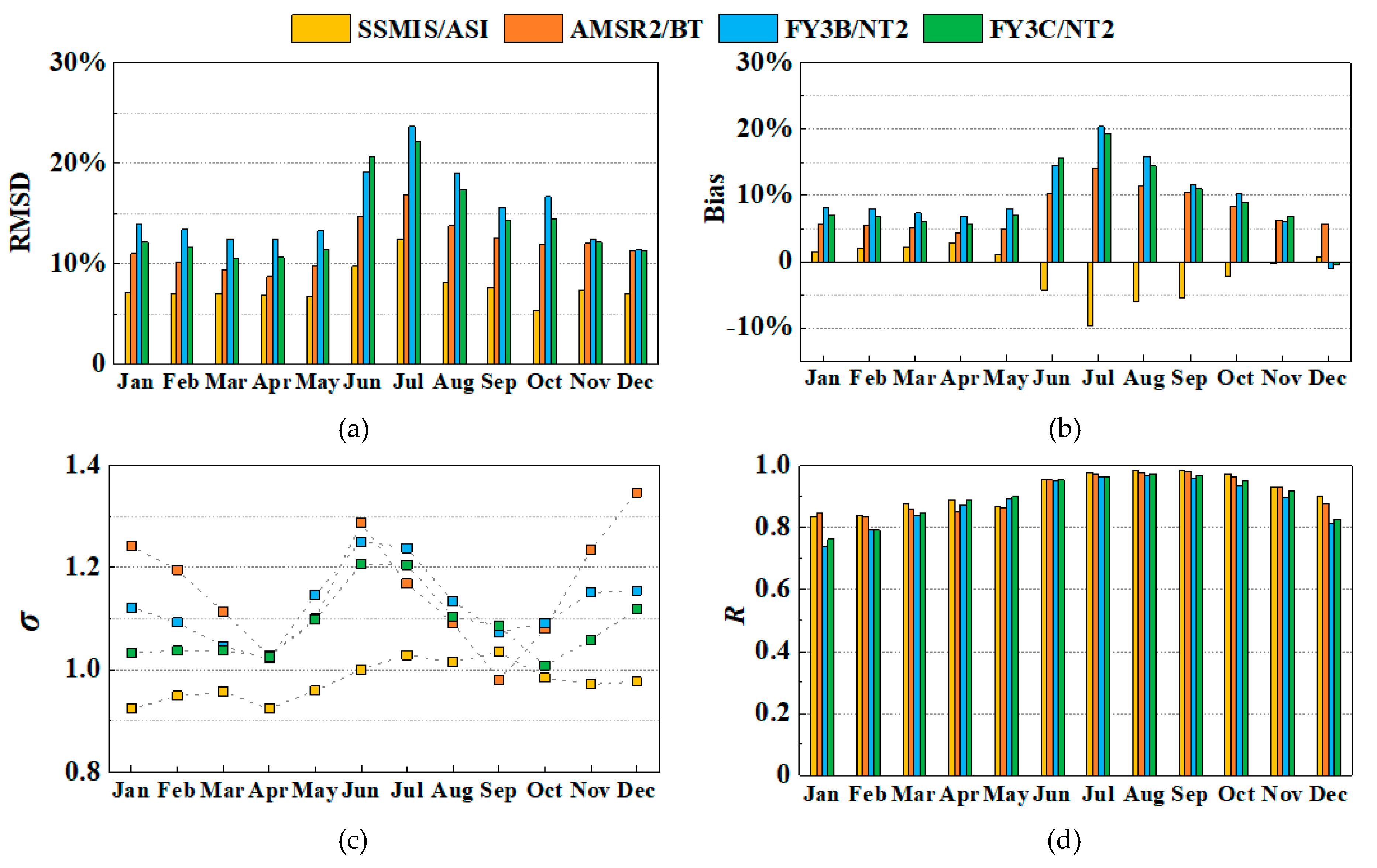
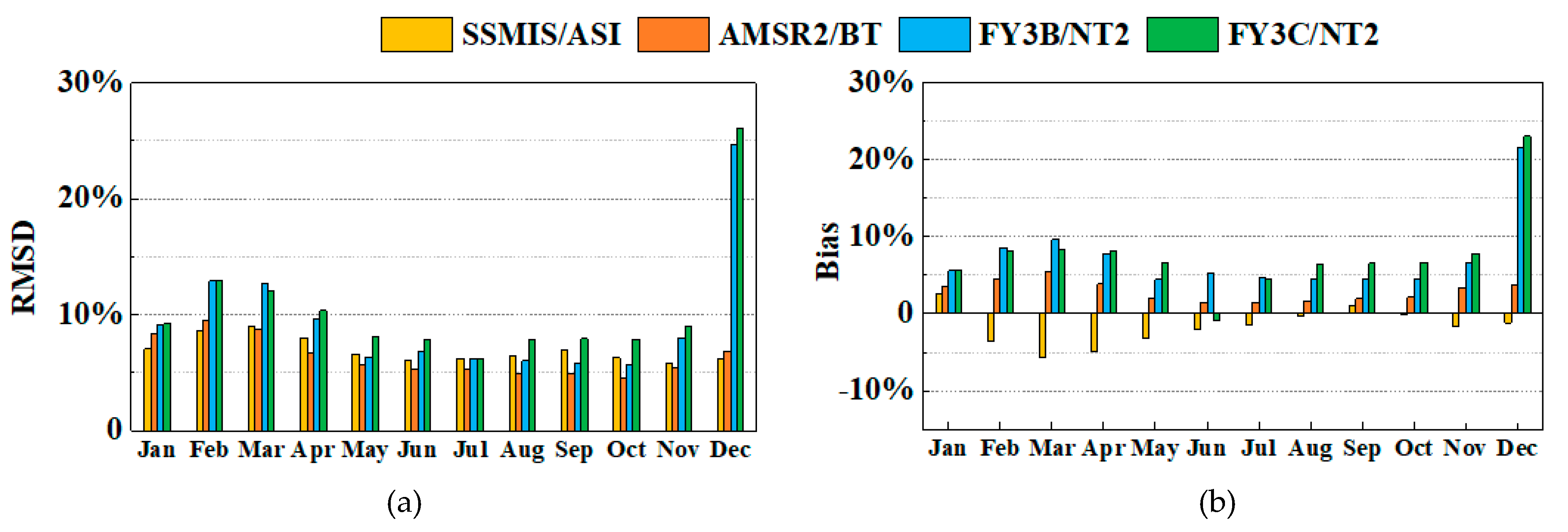
4.2. Comparison of PM SIC with ERA SIC

The monthly statistical metrics between the PM SIC and ERA SIC in Arctic are shown in Figure 3. As can be seen from Figure 3a,b, the RMSD and Bias values vary seasonally, and larger difference and inconsistency between PM SIC and ERA SIC substantially occur in July to September in Arctic region. The reason is that there is a large uncertainty in detecting sea ice by satellite observations during the sea ice melting season, due to the existence of snow melt pools on the sea ice surface in summer, which will influence the radiation signal received by microwave sensors [17]. The SSMIS/ASI has the lowest RMSD and Bias less than 10%, whereas the FY3 SIC products (particularly FY3B/NT2) show the largest RMSD compared to the other SIC products, with the RMSD even larger than 20% in June and July. Besides, the FY3 SIC and AMSR2/BT products continuously overestimate ERA SIC with a positive bias (except FY3 SIC products in December), whereas the SSMIS/ASI product underestimates ERA SIC in summer (July to September) and shows a very small positive bias in the remaining months. It should be mentioned that the archived grid resolution of ERA-Interim is in the reduced Gaussian grid N128/T255 [45], which is approximately 80 km in resolution. Therefore, there may be some uncertainties in the resampled ERA SIC (0.125°) used in the study.
The results indicate that different PM SIC algorithms have a notable different performance in summer. Meanwhile, we found that the monthly FY3/NT2 SIC are highest, followed by AMSR2/BT and SSMIS/ASI SIC. Besides, it can be seen from the standard deviation ratio in Figure 3c that the variation of the four PM SIC products with respect to that of ERA SIC is significant. The monthly fluctuation of the SSMIS/ASI product is smaller than that of the ERA SIC (i.e., σ < 1) at most of the time, while the fluctuations of the other three products are larger than ERA SIC. It also shows the fluctuation varies seasonally, with fewer fluctuations in April, September, and October. In addition, Figure 3d presents that all PM SIC products have a high correlation with ERA SIC (R > 0.73) in Arctic, which indicates that the PM SIC can well capture the temporal trend of ERA SIC.
Figure 4 shows the monthly SIC statistical metrics of four PM SIC in comparison with ERA SIC in the Antarctic. According to Figure 4a, the RMSD of PM SIC products varies seasonally, which is in line with the results in Arctic. The overall RMSD of AMSR2/BT is similar to that of SSMIS/ASI. The FY3 SIC products demonstrate the largest RMSD, especially in December (>20 %). Similar to the results of Arctic, the largest divergence between PM SIC and ERA SIC occurs in summer (January to March) except for FY3 SIC products in December, implying that there are still large uncertainties in SIC products in summer. Furthermore, the SSMIS/ASI product exhibits similar performance to that in Arctic by showing an underestimation of ERA SIC in summer, while the other three products still overestimate ERA SIC continuously. However, it is noted that the bias of the PM SIC is significantly lower than that of the Arctic region as detailed in Figure 4b. In addition, from the standard deviation ratio in Figure 4c, it is seen that the variation of the SSMIS/ASI product in May–November is smaller than that of ERA SIC, whereas the AMSR2/BT product exhibits the largest variation in general and the fluctuation of the FY3 SIC products is closest to that of ERA SIC during this period. Besides, as illustrated by Figure 4d, the monthly SIC of PM SIC products are highly consistent with ERA SIC in the Antarctic region with an average correlation coefficient higher than 0.85.
The statistical metrics of the four average monthly PM SIC products are summarized in Table 2. In Arctic region, the SSMIS/ASI product shows the lowest bias and RMSD of −1.46% and 7.7%, respectively, and the highest correlation coefficient of 0.92 relative to the ERA SIC. The FY3 SIC products have the largest bias and RMSD higher than 9.03% and 14.06%, respectively, but the correlation coefficients of both products are higher than 0.89, revealing the good temporal consistency of the two products with ERA SIC. The AMSR2/BT also shows good agreement with ERA SIC with a bias of 7.71% and a RMSD of 11.84%. In the Antarctic region, the FY3B/NT2, FY3C/NT2, and AMSR2/BT products all overestimate ERA SIC with a bias of 2.93%, 7.31%, and 7.55%, respectively, while the SSMIS/ASI underestimates ERA SIC with a bias of −2.13%. Similar phenomenon has also observed in Arctic. Overall, the variation in SSMIS/ASI product is slightly smaller than that in ERA SIC, while the fluctuations of the other three products are larger than ERA SIC in the whole polar region. All the four PM SIC products show a good temporal consistency with ERA SIC in the Arctic and Arctic regions, with an average correlation coefficient higher than 0.9 (expect FY3B/NT2 in Arctic with an R value of 0.89). Furthermore, to evaluate the consistency of PM SIC products in each season, the four error metrics in spring, summer, autumn, and winter in Arctic and Antarctic were calculated, also displayed in Table 2. In this study, April–June, July–September, October–December, and January–March were classified as spring, summer, autumn, and winter in Arctic, respectively [46], and October–December, January–March, April–June, July–September were classified as spring, summer, autumn, and winter in Antarctic, respectively [47]. The results clearly indicate that all the PM products exhibit the largest discrepancy to ERA SIC in summer in both Arctic and Antarctic except the results of FY3 SIC in Antarctic. The largest RMSD of FY3 SIC in spring in Antarctic is due to its abnormal behavior in December, which is shown in Figure 4b. Overall, the results of Table 2 and Figure 3 and Figure 4 indicate that large uncertainties exist in satellite SIC products in summer.
In summary, compared with ERA SIC, the SSMIS/ASI performs the best in Arctic but shows negative bias, while AMSR2/BT exhibits the highest absolute accuracy in Antarctic but overestimates SIC. The FY3/NT2 SIC products have the highest monthly SIC value leading to a relatively large positive bias, but they display good temporal consistency with ERA SIC. On average, the SSMIS/ASI shows the best agreement with ERA SIC in the whole polar regions, particularly in terms of RMSD and bias.

4.3. Comparison of Annual SIC

The statistical indicators between annual PM SIC products and ERA SIC in the period of 2015–2018 are shown in Figure 5. The four PM SIC products consistently present a similar spatial pattern in terms of RMSD, σ, and R. It is also found that the most noticeable discrepancy between PM and ERA SIC occurs in the marginal ice zone, with the RMSD larger than 20%, where the daily average SIC is below 20% (see in Figure 1). In these regions, all PM products also show large variations than ERA SIC with the standard deviation ratio (σ) larger than 1. In high concentration sea ice zones (the daily average SIC is above 90%), the RMSD and bias of PM SIC are smaller, indicating that the four PM SIC products are close to ERA SIC in these zones. In addition, the SSMIS/ASI has a negative bias in the Okhostsk Sea and high concentration sea ice zones, while the other PM SIC products present a positive bias. The discrepancies of RMSD among the AMSR2/BT, FY3B/NT2, and FY3C/NT2 are not apparent. The AMSR2/BT performs similarly with the FY3B/NT2 and FY3C/NT2 in terms of bias, and they all overestimate ERA SIC in most areas in the Arctic region. However, the PM SIC products all are highly correlate with ERA SIC. It should be noted that the lower correlation coefficient primary occurs in the zones near the Arctic center. This is because that the sea ice type in these zones is almost multiyear or perennial sea ice, and the variation of sea ice is much smaller in these regions than other areas.
The comparison results of annual SIC in Antarctic are presented in Figure 6. The comparisons indicate that the results in Antarctic are generally in line with those in Arctic, but the discrepancies between PM and ERA SIC are smaller in Antarctic. The spatial distribution of RMSD for the four PM SIC products is similar and the largest RMSD also occurs in the marginal ice zone. In this zone, the four PM SIC products all overestimate the ERA SIC and their bias is larger than that of other regions. Similarly, the PM products exhibit larger temporal variations than ERA SIC in the marginal ice zone. In terms of tracking temporal evolution of SIC, the four PM SIC products are all highly correlated with ERA SIC, with the R value higher than 0.6 in most areas. In the Weddell Sea, the RMSD and R are both the smallest as the multiyear sea ice is the main sea ice type in this zone. The sea ice nearly remains the same during the period, which leads to the highest absolute accuracy of PM SIC, but also the lowest correlation values due to the small variation of the sea ice in this region. The FY3C SIC products still overestimate ERA SIC clearly than the SSMIS/ASI and the AMSR2/BT in terms of bias.

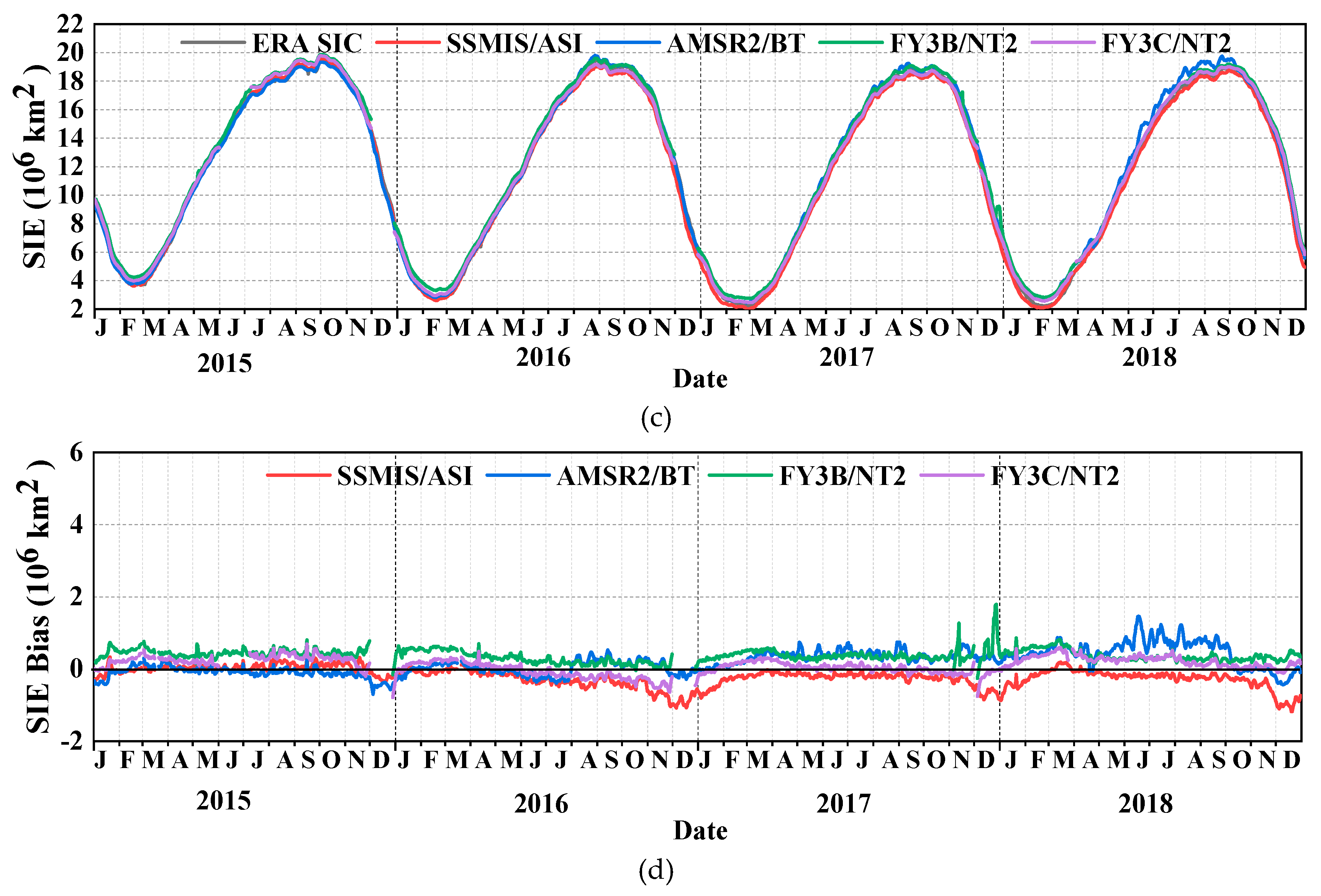
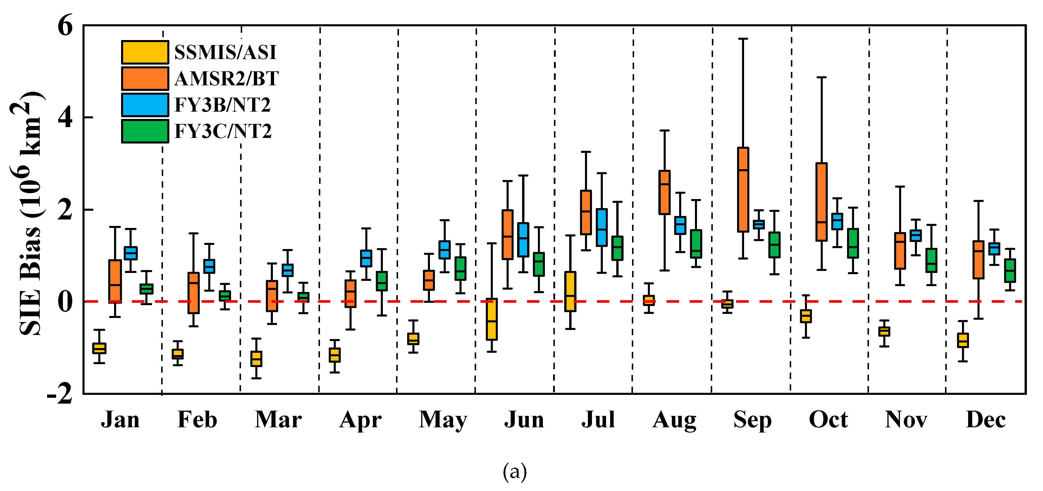
4.4. Comparison of Four PM Products Concerning the SIE

From Figure 7 it can be seen that the four PM SIC and ERA SIC all can reflect the variability of daily SIE in the whole polar region. For each product, the minimum/maximum SIE occurs in September/March in Arctic and in February/September in Antarctic. However, a fairly large difference in numerical values is noticed in these products. In the Arctic, it is evident that when the SIE is the largest, the SSMIS/ASI tends to underestimate ERA SIE, and when the SIE is small, the SSMIS/ASI product is closer to ERA SIE. The other three products all overestimate the minimum SIE (see Figure 7a).
In the Arctic, the SSMIS/ASI SIE mainly exhibits negative bias in comparison with ERA SIE, within ±2 × 10⁶ km2 (nearly ±13.33% of the investigated range). To be consistent with all products, we roughly used 15 × 106 km2 and 20 × 106 km2 as the range of measured values (corresponding to ERA data) for SIE in Arctic and Antarctic, respectively. The minimum SIE of the AMSR2/BT in 2016, 2017, and 2018 is larger than others and the AMSR2/BT significantly overestimates the SIE derived from ERA SIC, with a maximum daily bias reaches 5 × 10⁶ km2 (~33.33% of the investigated range). It may be ascribed to the more erroneous sea ice (SIC is greater than 15%) which results from the false sea ice caused by weather filtering [12]. The FY3B/NT2 remains similar SIE with the FY3C/NT2, but the FY3C/NT2 is closer to ERA SIE.
It can be observed in Figure 7c,d that all products exhibit very similar changes of SIE in Antarctic. Compared with the Arctic region, the differences in SIE derived from four PM SIC and ERA SIC are not significant, whose range is ~± 1 × 10⁶ km2 (nearly ±5% of the investigated range). The SSMIS/ASI and the AMSR2/BT SIE are the closest to ERA SIE, while the FY3 SIC has a higher SIE with a positive bias.
The SIE bias distribution of the four products in month is given in Figure 8. The SIE bias in the Arctic presents noticeable seasonal variation, and the large bias is mainly concentrated in July to October. In contrast, the SIE bias of PM products in the Antarctic is stable, and the range is within ±1 × 10⁶ km2 (nearly ±5% of the investigated range). Additionally, except the SSMIS/ASI, the other PM products all present positive SIE bias, illustrating that larger SIE was estimated by PM SIC products than ERA SIC. It is also seen from Figure 8a that the SSMIS/ASI has lower SIE than ERA in every month. The fluctuation of SIE bias of the AMSR2/BT is larger than other products in the whole polar region. Though the FY3 SIC products have the largest bias in December in Antarctic, there is no significant difference in SIE bias.
Table 3 provides the quantitative statistic metrics of the SIE derived from four PM SIC products in the whole polar region. In the Arctic region, the SSMIS/ASI is closest to the ERA SIE, with the lowest bias of −0.43 × 10⁶ km2 (nearly ±2.87% of the investigated range) and RMSD of 1.66 × 10⁶ km2 (nearly ±11.07% of the investigated range). On the contrary, in Antarctic region, the FY3C/NT2 shows the best agreement with the ERA SIE, with the lowest bias of 0.15 × 10⁶ km2 (nearly ±0.75% of the investigated range) and RMSD of 0.53 × 10⁶ km2 (nearly ±2.65% of the investigated range). Overall, the results indicate that the SIC product obtained by the same retrieval algorithm has different performance in different polar regions.

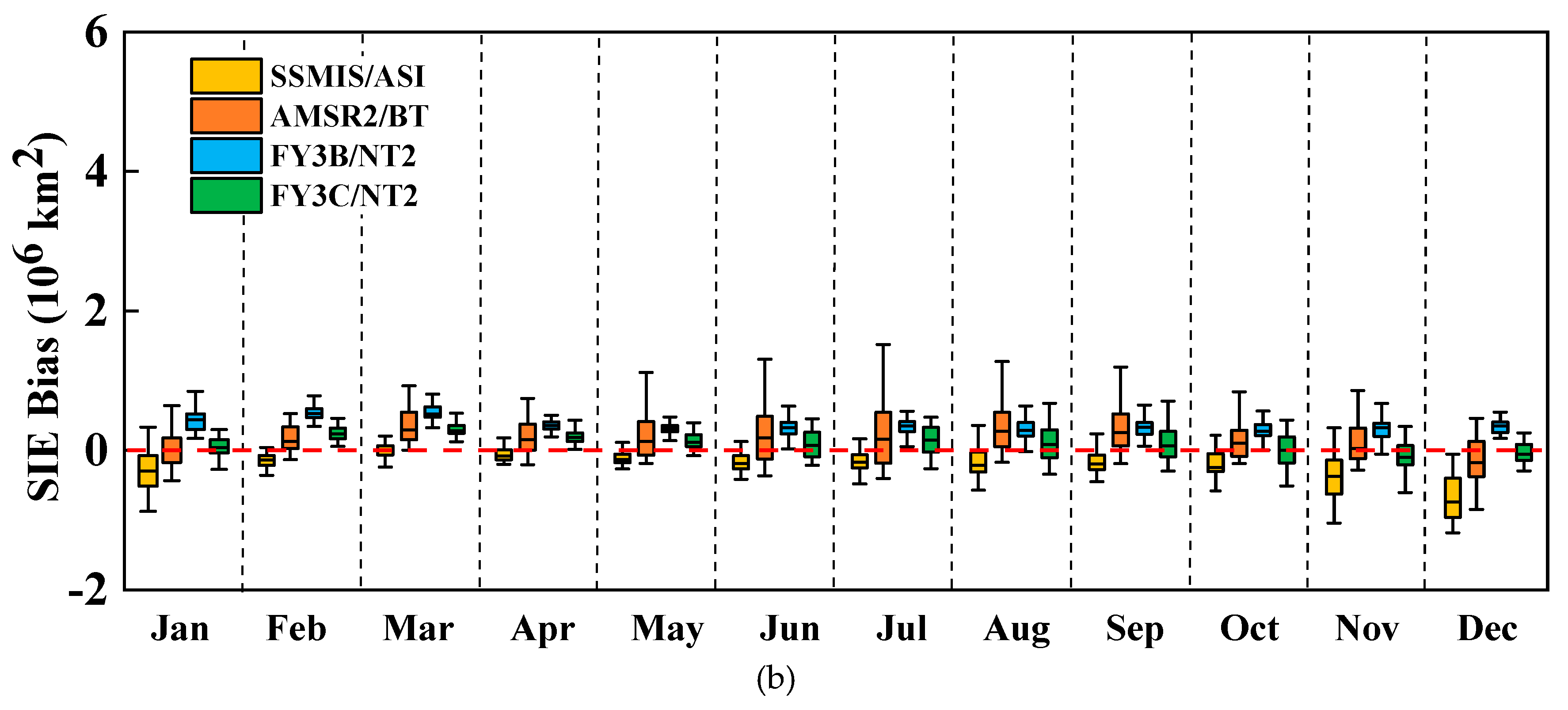
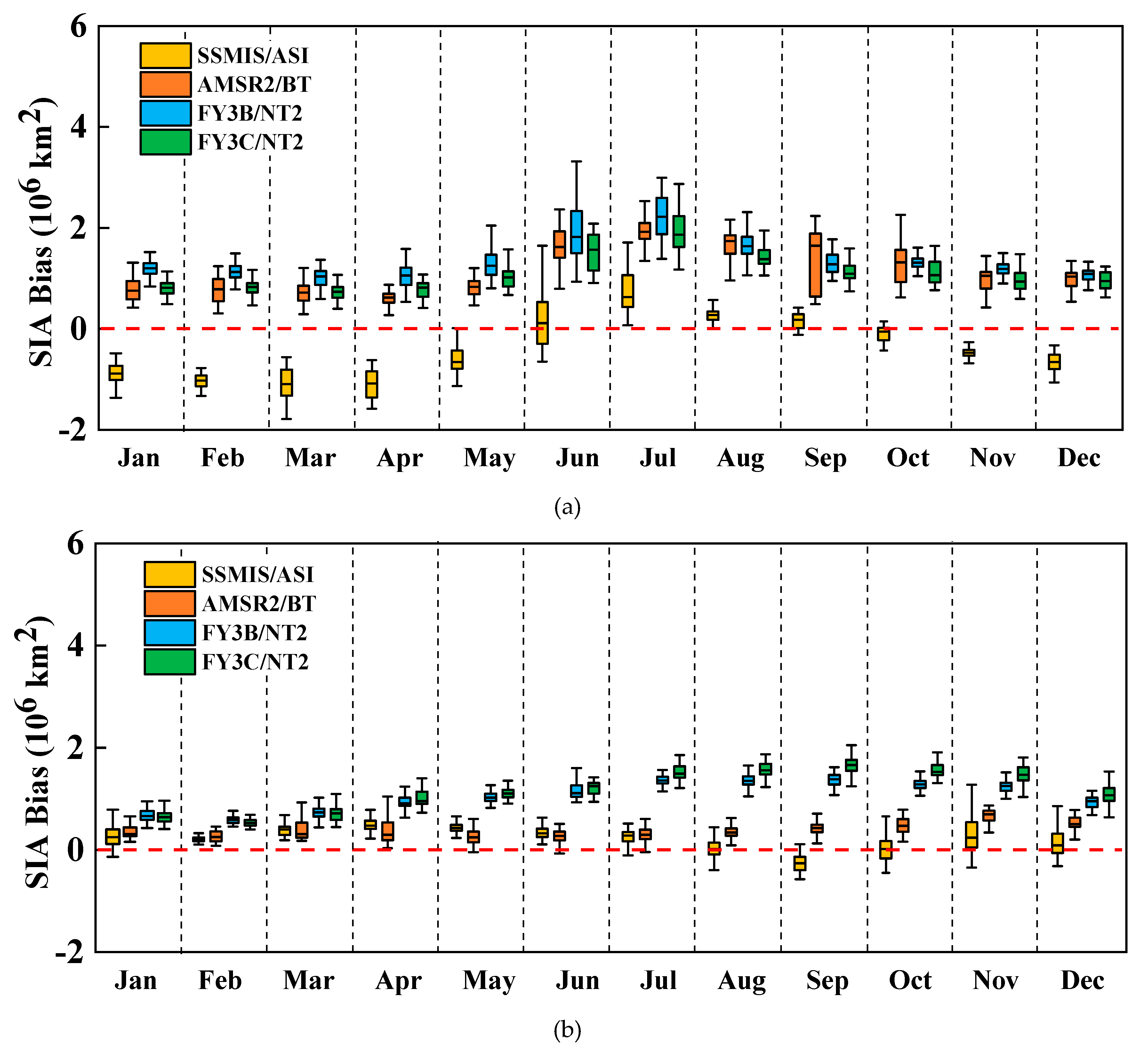
4.5. Comparison of Four PM Products Concerning the SIA

From Figure 9, it can be observed that the all PM and ERA data can well reflect the variability of daily SIA in polar regions, and the variations of SIA are slightly smoother than those of SIE. Moreover, the results indicate that the largest inconsistency between PM and ERA products locates at the maximum and minimum SIA in Arctic (see Figure 9a,b). The SSMIS/ASI exhibits the lowest SIA, while the FY3B/NT2 displays the largest SIA. From Figure 9b, it is seen that the range of bias is from −2 × 10⁶ km2 to 4 × 10⁶ km2 (nearly −14.29% to 28.57% of the investigated range). To be consistent with all products, we roughly used 14 × 106 km2 and 18 × 106 km2 as the range of measured values (corresponding to ERA data) for SIA in Arctic and Antarctic, respectively. The discrepancy of SIA in Antarctic is smaller than that in Arctic, and the largest discrepancy locates at maximum SIA. Figure 9d reveals that the FY3 SIC products have the largest positive bias, and the SSMIS/ASI and the AMSR2/BT have lower bias.
The SIA bias distribution of Arctic and Antarctic in month is shown in Figure 10. Similar to the results of SIE, the SIA bias varies seasonally in Arctic, with larger bias in June, July, and August for the AMSR2/BT and the FY3/NT2 SIC products, and from January to April for the SSMIS/ASI. Though the SIA bias in Antarctic also presents seasonal variation, its fluctuation is smaller than that in Arctic. The overall SIA bias is larger than SIE owing to the different SIC values estimated by different PM SIC algorithms. According to Figure 10a,b, we can find that the range of SIA bias is from −2 × 10⁶ km2 to 4 × 10⁶ km2 (−14.29% to 28.57% of the investigated range) and from −1 × 10⁶ km2 to 2×10⁶ km2 (−5.56% to 11.11% of the investigated range) in Arctic and Antarctic, respectively.
The error metrics of daily SIA between four PM and ERA data in the period of 2015–2018 are listed in Table 4. The SSMIS/ASI presents the overall lowest bias and RMSD among the four PM SIA, but it underestimates the ERA SIA in Arctic while overestimates ERA SIA in Antarctic. The AMSR2/BT is closer to ERA data than FY3C/NT2 and FY3B/NT2 with a lower RMSD in polar regions. In addition, the SIA calculated by the AMSR/BT and FY3/NT2 SIC products all overestimate the SIA derived from ERA SIC.

5. Discussion

In this study, we attempt to investigate the consistency of PM SIC products over the entire Arctic and Antarctic regions, and we also want to compare the performance of the new Chinese FY3 SIC products with other products. As no single satellite/sensor delivers all the products with different algorithms, we have chosen the four SIC products (SSMIS, AMSR2, FY3B, and FY3C) that derived from three well-established algorithms (ASI, BT, and NT2) with the same grid resolution. As the results shown in Section 4, although the four PM SIC products can generally well reflect the temporal and spatial pattern of sea ice, the discrepancy between PM and ERA SIC still exists in Arctic and Antarctic regions. It is necessary to investigate and discuss the possible error sources of the SIC retrievals, and the difference may be the results of combined effects of many factors, especially in the polar region with various sea ice types and conditions. First, in our study, the four PM SIC products are originated from three SIC retrieval algorithms (i.e., ASI, BT, and NT2), which adopts different retrieval schemes. The discrepancy of SIC can be attributed to the choice and utilization of different channels and weather filter approaches. It should be noted that a 5-day median filter was applied to the SSMIS/ASI product to remove spurious sea ice over open ocean and to reduce weather-induced elevated sea ice concentrations along the ice edge [48]. Thus, the differences of the SSMIS/ASI product compared to other datasets may be partially attributed to the nature of this dataset. Additionally, the brightness temperature acquired by different microwave radiometers (i.e., SSMIS, AMSR2, and MWRI), which have its own properties, are used in SIC algorithms, and the inter-sensor calibration discrepancies of brightness temperature can also lead to the discrepancies in SIC products.
The results indicate that larger bias of four PM SIC products in comparison with the ERA SIC occurs in summer, which is in line with previous studies [49,50]. The large uncertainty in SIC retrievals during the summer period is caused by increased variability in sea ice emissivity due to the surface wetness and presence of melt ponds. The performance of SIC algorithm heavily depends on sea ice conditions, particularly the surface melt and thin ice. Surface melt generally reduces concentration (the algorithm interprets the liquid water as open water) and thin ice is underestimated due to emission from the water beneath the ice [19]. Thin ice also occurs more commonly along the ice edge and satellite SIC algorithms usually have a low accuracy in those regions [35]. In our study, we also found that large inconsistency of the four products mainly occurs in the marginal ice zone, which is consistent with previous studies (see, e.g., in [17,29,33]). Ivanova et al. [17] reported that the areas with large uncertainty in PM SIC are often located at the marginal ice zone, which is caused by atmospheric contributions and wind roughening of open water areas. The marginal ice zone is also characterized by increased uncertainties due to smearing and footprint mismatch effects. Moreover, different algorithms use different combinations of frequency and polarization channels. The ASI algorithm only uses the high-frequency channel (e.g., 91 GHz for SSMIS and 89 GHz for AMSR2) to estimate SIC. At this high frequency, emission comes primarily from the snow or ice surface. Therefore, this channel is less sensitive to inhomogeneity in the snow or ice (particularly icy, refrozen layers within the snow) [29] compared with low-frequency channels, such as 19 GHz and 37 GHz used in the AMSR2 BT algorithm. Moreover, the spatial resolution becomes higher with the increase of observation frequency. Therefore, the nominal spatial resolution of SIC obtained by ASI algorithm is higher than that of BT and NT2 (if the same satellite/sensor is used), though they are usually resampled to the same grid resolution to facilitate the application of users. Due to the higher resolution, the ASI algorithm will more precisely detect the sea ice edge. Lower resolution (e.g., BT and NT2 SIC) may lead to a “smearing out” of the ice edge, leading to an overestimate of the edge [19]. However, higher frequency (e.g., 91 GHz for SSMIS) is more susceptible to atmospheric cloud liquid water and water vapor, which will impose a negative effect on brightness temperatures. This effect takes place more frequently in summer and early autumn at marginal ice zone [35]. The BT algorithm [12] is based on cluster analysis of the emissivity scatter plots for two frequencies (19 GHz and 37 GHz for AMSR2). Comiso, et al. [51] reported that the BT formulation tends to be less sensitive to thin ice and layering effects with a polarization signature. However, BT algorithm will be sensitive to anomalous volume scattering characteristics in the snow and sea ice. Overall, the low-frequency channels will respond more to changes in the sea ice, whereas the high-frequency channels (89/91 GHz) barely penetrate the typical snow cover [33]. For the NT2 algorithm, it is an enhancement to the original NT algorithm. The enhancements in NT2 algorithm include the incorporation of the high-frequency (89 GHz for AMSR2) channel to reduce sensitivity to surface inhomogeneity. Compared with ASI, which also incorporates the high-frequency channel, a radiative transfer model is employed in NT2 to correct the atmospheric contribution to the high-frequency brightness temperature. This is a unique feature of the NT2 algorithm. In general, each algorithm has its own advantages and limitations. Ivanova et al. [17] compared the skill of 13 SIC retrieval algorithms and pointed out that a hybrid approach is suggested to retrieve SIC globally.
Moreover, the divergence of the PM SIC products varies seasonally. This may be due to the fact that the ice consolidation in winter results in the values of the tie points and brightness temperature being stable. In contrast, this consolidation is easily destroyed by surface melt in summer [52]. This phenomenon can be attributed to the presence of melt ponds, which is already known to be a problem for most of the SIC algorithms [4]. Furthermore, our results reveal that the same SIC product has different performance in the Arctic and Antarctic. In general, the uncertainty and discrepancy in Arctic is more pronounced than in Antarctic. It is known that there are different ice types and ice conditions in the Arctic and Antarctic. To simplify the inversion process, the sea ice in Arctic is widely identified as two types, i.e., the multiyear sea ice and first-year sea ice, whereas in Antarctic the sea ice is classified into types A and B [10], [51]. The presence of complex ice types (e.g., young ice, new ice, and floe, etc.) makes the PM SIC products more uncertain in Arctic than Antarctic. For this reason, the discrepancy of SIE and SIA is not significant especially for the Antarctic. The discrepancy in SIE and SIA is also likely related to the difference in land mask used in the algorithms. Since a fully independent with high-quality and hemisphere-wide SIC product does not exist, we adopted the ERA SIC to compare the consistency of PM SIC products in long-time series for the whole polar region. We acknowledge that there are still some errors and uncertainties in the ERA SIC product, and the work presented here is more appropriately treated as a comparison and not a validation work. We believe that the inconsistencies between different types of SIC products found in our study can assist in identifying potential problems with PM SIC products highlighting areas for improvement. It is also noteworthy that it is not our intention to conclude which algorithm (or product) is the best choice in the whole polar regions. The PM SIC algorithms are still under refinement and we expect these valuable satellite products can evolve and advance through positive comparison.

6. Conclusions

The quality and consistency of the satellite PM SIC products need to be examined for their applications and improvement. In this study, the consistency of PM products concerning daily/monthly/annual SIC as well as daily SIE and SIA were compared and evaluated with a reanalysis SIC product (i.e., ERA-Interim) in long time series (from 2015–2018) and the whole polar region. Moreover, the performance of the new Chinese FY3 SIC products was examined, which is being considered to integrate into the ESA CCI sea ice product [53]. These comparisons yield a better understanding of remotely sensed SIC products, which is conducive to the improvement of the SIC retrieval algorithms.
Overall, the spatial patterns of PM SIC products agree well with ERA SIC. The comparison of monthly and annual SIC shows that the largest bias and RMSD (even >20%) for the PM SIC products mainly occur in summer and the marginal ice zone, indicating that there are still many uncertainties in PM SIC products in such period and region. Meanwhile, the daily SIE and SIA derived from the four PM SIC products can generally well reflect the variation trend of SIE and SIA in Arctic and Antarctic. However, the largest bias of SIE and SIA are above 4×10⁶ km2 when the sea ice reaches the maximum and minimum value. Besides, the daily bias of SIE and SIA vary seasonally and regionally, which is particularly concentrated from June to October in the Arctic. The results of monthly and annual SIC are consistent with those of daily SIE and SIA. Generally, our results show that, among the four PM SIC products, the SSMIS/ASI product is closest to ERA SIC in the Arctic but it usually underestimates SIC with a negative bias, while the AMSR2/BT product exhibits the best consistency in Antarctic relative to ERA SIC but it overestimates SIC with a positive bias. The consistency of the four PM products with respect to ERA SIC in the Antarctic region is generally superior to that in Arctic. On average, the SIC, SIE and SIA derived from SSMIS/ASI are in the best agreement with ERA data.
In the future, the hybrid of multiple SIC algorithms can be considered, which will further improve the accuracy of the SIC retrievals. To further understand the accuracy of the PM SIC products, based on the findings in the study especially the inconsistency among the products, we will take SAR and optical images into account to ascertain regional uncertainties in the satellite-based SIC products in the next stage.

Author Contributions

Conceptualization, S.L. and J.Z.; Methodology, S.L. and J.Z.; Software, S.L. and D.Q.; Validation, S.L. and J.Z.; Formal Analysis, S.L., J.Z and Z.L.; investigation, J.Z.; Resources, J.Z; Data Curation, S.L.; Writing—Original Draft Preparation, S.L., J.Z., and D.Q.; Writing—Review & Editing, J.Z, P.Z., and H.B.; Visualization, S.L. and D.Q.; Supervision, Z.L.; Project Administration, Z.L. and J.Z.; Funding Acquisition, Z.L. and J.Z. All authors have read and agreed to the published version of the manuscript.

Funding

This research was funded by the National Key Research and Development Program of China (No. 2018YFA0605403). Jiangyuan Zeng was supported by the Youth Innovation Promotion Association CAS (No. 2018082).

Acknowledgments

The authors thank the four anonymous reviewers for their helpful reviews and suggestions. The authors also thank the University of Hamburg, University of Bremen, and CNSMC for providing the satellite SIC products, and the ECMWF for providing the ERA-Interim dataset.

Conflicts of Interest

The authors declare no conflict of interest.

References

  1. Johannessen, O.M.; Bengtsson, L.; Miles, M.W.; Kuzmina, S.I.; Semenov, V.A.; Alekseev, G.V.; Nagurnyi, A.P.; Zakharov, V.F.; Bobylev, L.P.; Pettersson, L.H. Arctic climate change: Observed and modelled temperature and sea-ice variability. Tellus A Dyn. Meteorol. Oceanogr. 2004, 56, 328–341. [Google Scholar] [CrossRef]
  2. Hurrell, J.W.; Hack, J.J.; Shea, D.; Caron, J.M.; Rosinski, J. A new sea surface temperature and sea ice boundary dataset for the Community Atmosphere Model. J. Clim. 2008, 21, 5145–5153. [Google Scholar] [CrossRef]
  3. Mahlstein, I.; Knutti, R. September Arctic sea ice predicted to disappear near 2 C global warming above present. J. Geophys. Res. Atmos. 2012, 117. [Google Scholar] [CrossRef]
  4. Han, H.; Kim, H.-C. Evaluation of summer passive microwave sea ice concentrations in the Chukchi Sea based on KOMPSAT-5 SAR and numerical weather prediction data. Remote Sens. Environ. 2018, 209, 343–362. [Google Scholar] [CrossRef]
  5. Deser, C.; Teng, H. Evolution of Arctic sea ice concentration trends and the role of atmospheric circulation forcing, 1979–2007. Geophys. Res. Lett. 2008, 35. [Google Scholar] [CrossRef] [Green Version]
  6. Budikova, D. Role of Arctic sea ice in global atmospheric circulation: A review. Glob. Planet. Chang. 2009, 68, 149–163. [Google Scholar] [CrossRef]
  7. Stroeve, J.C.; Serreze, M.C.; Holland, M.M.; Kay, J.E.; Malanik, J.; Barrett, A.P. The Arctic’s rapidly shrinking sea ice cover: A research synthesis. Clim. Chang. 2012, 110, 1005–1027. [Google Scholar] [CrossRef] [Green Version]
  8. Simpkins, G.R.; Ciasto, L.M.; Thompson, D.W.; England, M.H. Seasonal relationships between large-scale climate variability and Antarctic sea ice concentration. J. Clim. 2012, 25, 5451–5469. [Google Scholar] [CrossRef] [Green Version]
  9. Parkinson, C.L. A 40-y record reveals gradual Antarctic sea ice increases followed by decreases at rates far exceeding the rates seen in the Arctic. Proc. Natl. Acad. Sci. USA 2019, 116, 14414–14423. [Google Scholar] [CrossRef] [Green Version]
  10. Cavalieri, D.J.; Gloersen, P.; Campbell, W.J. Determination of sea ice parameters with the Nimbus 7 SMMR. J. Geophys. Res. Atmos. 1984, 89, 5355–5369. [Google Scholar] [CrossRef]
  11. Markus, T.; Cavalieri, D.J. An enhancement of the NASA Team sea ice algorithm. IEEE Trans. Geosci. Remote Sens. 2000, 38, 1387–1398. [Google Scholar] [CrossRef] [Green Version]
  12. Comiso, J.C. Characteristics of Arctic winter sea ice from satellite multispectral microwave observations. J. Geophys. Res. Ocean. 1986, 91, 975–994. [Google Scholar] [CrossRef]
  13. Kaleschke, L.; Lüpkes, C.; Vihma, T.; Haarpaintner, J.; Bochert, A.; Hartmann, J.; Heygster, G. SSM/I sea ice remote sensing for mesoscale ocean-atmosphere interaction analysis. Can. J. Remote Sens. 2001, 27, 526–537. [Google Scholar] [CrossRef]
  14. Spreen, G.; Kaleschke, L.; Heygster, G. Sea ice remote sensing using AMSR-E 89-GHz channels. J. Geophys. Res. Ocean. 2008, 113. [Google Scholar] [CrossRef] [Green Version]
  15. Breivik, L.-A.; Eastwood, S.; Godøy, Ø.; Schyberg, H.; Andersen, S.; Tonboe, R. Sea ice products for EUMETSAT satellite application facility. Can. J. Remote Sens. 2001, 27, 403–410. [Google Scholar] [CrossRef]
  16. Tonboe, R.; Lavelle, J.; Pfeiffer, R.-H.; Howe, E. Product User Manual for OSI SAF Global Sea Ice Concentration; Danish Meteorological Institute: Copenhagen, Denmark, 2016. [Google Scholar]
  17. Ivanova, N.; Pedersen, L.; Tonboe, R.; Kern, S.; Heygster, G.; Lavergne, T.; Sørensen, A.; Saldo, R.; Dybkjær, G.; Brucker, L. Inter-comparison and evaluation of sea ice algorithms: Towards further identification of challenges and optimal approach using passive microwave observations. Cryosphere 2015, 9, 1797–1817. [Google Scholar] [CrossRef] [Green Version]
  18. Meier, W.N.; Fetterer, F.; Stewart, J.S.; Helfrich, S. How do sea-ice concentrations from operational data compare with passive microwave estimates? Implications for improved model evaluations and forecasting. Ann. Glaciol. 2015, 56, 332–340. [Google Scholar] [CrossRef] [Green Version]
  19. Meier, W.N.; Stewart, J.S. Assessing uncertainties in sea ice extent climate indicators. Environ. Res. Lett. 2019, 14, 035005. [Google Scholar] [CrossRef]
  20. Wiebe, H.; Heygster, G.; Markus, T. Comparison of the ASI ice concentration algorithm with Landsat-7 ETM+ and SAR imagery. IEEE Trans. Geosci. Remote Sens. 2009, 47, 3008–3015. [Google Scholar] [CrossRef]
  21. Cavalieri, D.J.; Markus, T.; Hall, D.K.; Ivanoff, A.; Glick, E. Assessment of AMSR-E Antarctic winter sea-ice concentrations using Aqua MODIS. IEEE Trans. Geosci. Remote Sens. 2010, 48, 3331–3339. [Google Scholar] [CrossRef]
  22. Shi, L.; Lu, P.; Cheng, B.; Karvonen, J.; Wang, Q.; Li, Z.; Han, H. An assessment of arctic sea ice concentration retrieval based on “HY-2” scanning radiometer data using field observations during CHINARE-2012 and other satellite instruments. Acta Oceanol. Sin. 2015, 34, 42–50. [Google Scholar] [CrossRef]
  23. Ji, Q.; Li, F.; Pang, X.; Luo, C. Statistical analysis of SSMIS sea ice concentration threshold at the Arctic Sea Ice Edge during summer based on MODIS and ship-based observational data. Sensors 2018, 18, 1109. [Google Scholar] [CrossRef] [PubMed] [Green Version]
  24. Knuth, M.A.; Ackley, S.F. Summer and early-fall sea-ice concentration in the Ross Sea: Comparison of in situ ASPeCt observations and satellite passive microwave estimates. Ann. Glaciol. 2006, 44, 303–309. [Google Scholar] [CrossRef] [Green Version]
  25. Ozsoy-Cicek, B.; Xie, H.; Ackley, S.; Ye, K. Antarctic summer sea ice concentration and extent: Comparison of ODEN 2006 ship observations, satellite passive microwave and NIC sea ice charts. Cryosphere 2009, 3, 1. [Google Scholar] [CrossRef] [Green Version]
  26. Zhao, X.; Su, H.; Stein, A.; Pang, X. Comparison between AMSR-E ASI sea-ice concentration product, MODIS and pseudo-ship observations of the Antarctic sea-ice edge. Ann. Glaciol. 2015, 56, 45–52. [Google Scholar] [CrossRef] [Green Version]
  27. Steffen, K.; Schweiger, A. NASA team algorithm for sea ice concentration retrieval from Defense Meteorological Satellite Program special sensor microwave imager: Comparison with Landsat satellite imagery. J. Geophys. Res. Ocean. 1991, 96, 21971–21987. [Google Scholar] [CrossRef]
  28. Kern, S.; Kaleschke, L.; Clausi, D.A. A comparison of two 85-GHz SSM/I ice concentration algorithms with AVHRR and ERS-2 SAR imagery. IEEE Trans. Geosci. Remote Sens. 2003, 41, 2294–2306. [Google Scholar] [CrossRef]
  29. Meier, W.N. Comparison of passive microwave ice concentration algorithm retrievals with AVHRR imagery in Arctic peripheral seas. IEEE Trans. Geosci. Remote Sens. 2005, 43, 1324–1337. [Google Scholar] [CrossRef]
  30. Cavalieri, D.J.; Markus, T.; Hall, D.K.; Gasiewski, A.J.; Klein, M.; Ivanoff, A. Assessment of EOS Aqua AMSR-E Arctic sea ice concentrations using Landsat-7 and airborne microwave imagery. IEEE Trans. Geosci. Remote Sens. 2006, 44, 3057–3069. [Google Scholar] [CrossRef]
  31. Heinrichs, J.F.; Cavalieri, D.J.; Markus, T. Assessment of the AMSR-E Sea Ice-Concentration product at the ice edge using RADARSAT-1 and MODIS imagery. IEEE Trans. Geosci. Remote Sens. 2006, 44, 3070–3080. [Google Scholar] [CrossRef]
  32. Shokr, M.; Markus, T. Comparison of NASA Team2 and AES-York ice concentration algorithms against operational ice charts from the Canadian ice service. IEEE Trans. Geosci. Remote Sens. 2006, 44, 2164–2175. [Google Scholar] [CrossRef]
  33. Andersen, S.; Tonboe, R.; Kaleschke, L.; Heygster, G.; Pedersen, L.T. Intercomparison of passive microwave sea ice concentration retrievals over the high-concentration Arctic sea ice. J. Geophys. Res. Ocean. 2007, 112. [Google Scholar] [CrossRef]
  34. Hao, G.; Su, J. A study on the dynamic tie points ASI algorithm in the Arctic Ocean. Acta Oceanol. Sin. 2015, 34, 126–135. [Google Scholar] [CrossRef]
  35. Pang, X.; Pu, J.; Zhao, X.; Ji, Q.; Qu, M.; Cheng, Z. Comparison between AMSR2 sea ice concentration products and pseudo-ship observations of the Arctic and Antarctic sea ice edge on cloud-free days. Remote Sens. 2018, 10, 317. [Google Scholar] [CrossRef] [Green Version]
  36. Svendsen, E.; Matzler, C.; Grenfell, T.C. A model for retrieving total sea ice concentration from a spaceborne dual-polarized passive microwave instrument operating near 90 GHz. Int. J. Remote Sens. 1987, 8, 1479–1487. [Google Scholar] [CrossRef]
  37. Kern, S.; Kaleschke, L.; Spreen, G. Climatology of the Nordic (Irminger, Greenland, Barents, Kara and White/Pechora) Seas ice cover based on 85 GHz satellite microwave radiometry: 1992–2008. Tellus A Dyn. Meteorol. Oceanogr. 2010, 62, 411–434. [Google Scholar] [CrossRef]
  38. Dee, D.P.; Uppala, S.M.; Simmons, A.; Berrisford, P.; Poli, P.; Kobayashi, S.; Andrae, U.; Balmaseda, M.; Balsamo, G.; Bauer, d.P. The ERA-Interim reanalysis: Configuration and performance of the data assimilation system. Q. J. R. Meteorol. Soc. 2011, 137, 553–597. [Google Scholar] [CrossRef]
  39. Eastwood, S.; Larsen, K.; Lavergne, T.; Neilsen, E.; Tonboe, R. OSI SAF Global Sea Ice Concentration Reprocessing: Product User Manual, Version 1.3; EUMETSAT OSI SAF (Product 0SIOSI-409): Darmstadt, Germany, 2011. [Google Scholar]
  40. Zeng, J.; Li, Z.; Chen, Q.; Bi, H.; Qiu, J.; Zou, P. Evaluation of remotely sensed and reanalysis soil moisture products over the Tibetan Plateau using in-situ observations. Remote Sens. Environ. 2015, 163, 91–110. [Google Scholar] [CrossRef]
  41. Cavalieri, D.J.; Parkinson, C.L. Arctic sea ice variability and trends, 1979–2010. Cryosphere 2012, 6, 881. [Google Scholar] [CrossRef] [Green Version]
  42. Bjorgo, E.; Johannessen, O.M. Sea ice concentrations derived from SMMR and SSMI: Parameter retrieval and algorithm evaluation. Proceedings of Oceanic Remote Sensing and Sea Ice Monitoring, Rome, Italy, 21 December 1994; pp. 114–125. [Google Scholar]
  43. Cavalieri, D.; Crawford, J.; Drinkwater, M.; Eppler, D.; Farmer, L.; Jentz, R.; Wackerman, C. Aircraft active and passive microwave validation of sea ice concentration from the Defense Meteorological Satellite Program Special Sensor Microwave Imager. J. Geophys. Res. Ocean. 1991, 96, 21989–22008. [Google Scholar] [CrossRef]
  44. Hauke, J.; Kossowski, T. Comparison of values of Pearson’s and Spearman’s correlation coefficients on the same sets of data. Quaest. Geogr. 2011, 30, 87–93. [Google Scholar] [CrossRef] [Green Version]
  45. Berrisford, P.; Dee, D.; Poli, P.; Brugge, R.; Fielding, K.; Fuentes, M.; Kallberg, P.; Kobayashi, S.; Uppala, S.; Simmons, A. The ERA-Interim Archive Version 2.0. Available from ECMWF Technical Report; ECMWF, Shinfield Park: Reading, UK, 2011. [Google Scholar]
  46. Wang, Y.; Bi, H.; Huang, H.; Liu, Y.; Liu, Y.; Liang, X.; Fu, M.; Zhang, Z. Satellite-observed trends in the Arctic sea ice concentration for the period 1979–2016. J. Oceanol. Limnol. 2019, 37, 18–37. [Google Scholar] [CrossRef]
  47. Shi, Q.; Yang, Q.; Mu, L.; Wang, J.; Massonnet, F.; Mazloff, M. Evaluation of Sea-Ice Thickness from four reanalyses in the Antarctic Weddell Sea. Cryosphere Discuss. 2020, 1–31. [Google Scholar] [CrossRef] [Green Version]
  48. Kern, S.; Lavergne, T.; Notz, D.; Pedersen, L.T.; Tonboe, R.T.; Saldo, R.; Sorensen, M. Satellite passive microwave sea-ice concentration data set intercomparison: Closed ice and ship-based observations. Cryosphere 2019, 13, 3261–3307. [Google Scholar] [CrossRef] [Green Version]
  49. Meier, W.; Notz, D. A note on the accuracy and reliability of satellite-derived passive microwave estimates of sea-ice extent. In Clic Arctic Sea Ice Working Group Consensus Document; World Climate Research Program: Case Postale, Switzerland, 2010. [Google Scholar]
  50. Ivanova, N.; Johannessen, O.M.; Pedersen, L.T.; Tonboe, R.T. Retrieval of Arctic sea ice parameters by satellite passive microwave sensors: A comparison of eleven sea ice concentration algorithms. IEEE Trans. Geosci. Remote Sens. 2014, 52, 7233–7246. [Google Scholar] [CrossRef]
  51. Comiso, J.C.; Cavalieri, D.J.; Parkinson, C.L.; Gloersen, P. Passive microwave algorithms for sea ice concentration: A comparison of two techniques. Remote Sens. Environ. 1997, 60, 357–384. [Google Scholar] [CrossRef]
  52. Liu, T.; Liu, Y.; Huang, X.; Wang, Z. Fully constrained least squares for antarctic sea ice concentration estimation utilizing passive microwave data. IEEE Geosci. Remote Sens. Lett. 2015, 12, 2291–2295. [Google Scholar] [CrossRef]
  53. Lavergne, T.; Sørensen, A.M.; Kern, S.; Tonboe, R.; Notz, D.; Aaboe, S.; Bell, L.; Dybkjær, G.; Eastwood, S.; Gabarro, C. Version 2 of the EUMETSAT OSI SAF and ESA CCI sea-ice concentration climate data records. Cryosphere 2019, 13, 49–78. [Google Scholar] [CrossRef] [Green Version]
Figure 1. Daily average PM and ERA-Interim sea ice fraction data (ERA SIC) products in the period of 2015–2018 in Arctic.
Remotesensing 12 02880 g001
Figure 2. Daily average PM and ERA SIC products in the period of 2015–2018 in Antarctic.
Remotesensing 12 02880 g002
Figure 3. Monthly SIC error metrics between PM SIC products and ERA SIC in the period of 2015–2018 in the Arctic region for (a) root mean square difference (RMSD), (b) bias, (c) σ, and (d) R.
Remotesensing 12 02880 g003
Figure 4. Monthly SIC error metrics between PM SIC products and ERA SIC in the period of 2015–2018 in the Antarctic region for (a) RMSD, (b) bias, (c) σ, and (d) R.
Remotesensing 12 02880 g004aRemotesensing 12 02880 g004b
Figure 5. Statistical indicators between annual PM SIC products and ERA SIC in the period of 2015–2018 in Arctic region for (a) RMSD, (b) bias, (c) σ, and (d) R.
Remotesensing 12 02880 g005
Figure 6. Statistical indicators between annual PM SIC products and ERA SIC in the period of 2015–2018 in Antarctic region for (a) RMSD, (b) bias, (c) σ, and (d) R.
Remotesensing 12 02880 g006
Figure 7. Temporal evolution of daily SIE and its bias between four PM SIC and ERA SIC in the period of 2015–2018 in Arctic and Antarctic for (a) SIE in Arctic, (b) SIE bias in Arctic, (c) SIE in Antarctic, and (d) SIE bias in Antarctic.
Remotesensing 12 02880 g007aRemotesensing 12 02880 g007b
Figure 8. The SIE bias regarding comparison between PM SIC and ERA SIC in every month during the period of 2015–2018 for (a) Arctic and (b) Antarctic.
Remotesensing 12 02880 g008aRemotesensing 12 02880 g008b
Figure 9. Temporal evolution of daily SIA and its bias between four PM SIC and ERA SIC in the period of 2015–2018 in Arctic and Antarctic for (a) SIA in Arctic, (b) SIA bias in Arctic, (c) SIA in Antarctic, and (d) SIA bias in Antarctic.
Remotesensing 12 02880 g009
Figure 10. The SIA bias regarding the comparison between PM SIC and ERA SIC during the period of 2015-2018 for (a) Arctic and (b) Antarctic.
Remotesensing 12 02880 g010
Table 1. The main information of the passive microwave sea ice concentration (PM SIC) products used in the study.
ProductsGrid ResolutionAlgorithmSensorFrequencySource
SSMIS/ASI12.5 kmASISSMIS91 V, 91 HUniversity of Hamburg
AMSR2/BT12.5 kmBTAMSR219V, 37VUniversity of Bremen
FY3B/NT212.5 kmNT2MWRI19V, 19H, 37V, 89 H, 89 VNational Satellite Meteorological Centre
FY3C/NT212.5 kmNT2MWRI19V, 19H, 37V, 89 H, 89 VNational Satellite Meteorological Centre
Table 2. Error metrics of monthly SIC between four PM SIC and ERA SIC in the period of 2015–2018. RMSD and bias are in %. σ is the standard deviation ratio and R is the correlation coefficient (p-value < 0.01). N is the number of samples. April–June, July–September, October–December, and January–March were classified as spring, summer, autumn, and winter in Arctic, respectively, and October–December, January–March, April–June, July–September were classified as spring, summer, autumn, and winter in Antarctic, respectively.
SeasonProductsArcticAntarctic
RMSDBiasσRNRMSDBiasσRN
SpringSSMIS/ASI6.92−0.090.960.90246,5756.10−0.970.960.96368,938
AMSR2/BT11.266.531.140.89263,3865.583.081.060.98375,966
FY3B/NT211.359.831.140.91253,97412.7710.911.040.97374,912
FY3C/NT211.279.481.110.91253,45214.3312.491.070.97373,897
SummerSSMIS/ASI9.39−7.081.030.98141,2178.25−2.181.040.97140,258
AMSR2/BT14.4112.081.080.98150,8278.864.511.040.97143,170
FY3B/NT219.4215.961.150.96144,84511.587.941.100.97144,345
FY3C/NT217.9714.931.130.97144,85511.427.331.110.97142,590
AutumnSSMIS/ASI6.55−0.590.980.94195,0666.91−3.410.980.95262,077
AMSR2/BT11.736.771.220.92210,3025.862.431.060.98267,057
FY3B/NT213.475.061.130.88201,1127.615.841.050.97266,609
FY3C/NT212.625.091.060.90199,9568.804.561.060.96263,247
WinterSSMIS/ASI7.051.910.940.85281,2836.55−0.190.890.86405,259
AMSR2/BT10.175.431.180.85302,7015.061.681.150.94413,891
FY3B/NT213.297.821.080.80290,5746.024.561.020.94412,003
FY3C/NT211.426.631.040.80288,8957.325.801.020.94409,887
AllSSMIS/ASI7.70−1.460.980.92864,1416.95−2.130.970.931,176,532
AMSR2/BT11.847.711.160.91927,2166.342.931.080.971,200,084
FY3B/NT215.299.671.130.89890,5059.507.311.050.961,197,869
FY3C/NT214.069.031.090.90887,15810.497.551.070.961,189,621
Table 3. Error metrics of daily SIE derived from four PM SIC with respect to ERA data in the period of 2015–2018. RMSD and bias are in 106 km2. R is the correlation coefficient (p-value < 0.01).
ProductsArcticAntarctic
BiasRMSDRBiasRMSDR
SSMIS/ASI−0.431.660.93−0.170.540.99
AMSR2/BT1.362.450.920.220.590.99
FY3B/NT21.462.190.930.420.650.99
FY3C/NT20.941.900.930.150.530.99
Table 4. Error metrics of daily SIA between four PM SIC and ERA SIC in the period of 2015–2018. RMSD and Bias are in 106 km2. R is the correlation coefficient (p-value < 0.01).
ProductsArcticAntarctic
BiasRMSDRBiasRMSDR
SSMIS/ASI−0.231.480.930.260.500.99
AMSR2/BT1.271.900.940.420.540.99
FY3B/NT21.532.120.921.101.170.99
FY3C/NT21.251.930.931.221.310.99

