Detecting Classic Maya Settlements with Lidar-Derived Relief Visualizations

1
The Field Museum of Natural History, Chicago, IL 60605, USA
2
Department of Geography and the Environment, University of Texas at Austin, Austin, TX 78712, USA
Remote Sens. 2020, 12(17), 2838; https://doi.org/10.3390/rs12172838
Submission received: 4 July 2020
/
Revised: 22 August 2020
/
Accepted: 29 August 2020
/
Published: 1 September 2020
Abstract
:In the past decade, Light Detection and Ranging (lidar) has fundamentally changed our ability to remotely detect archaeological features and deepen our understanding of past human-environment interactions, settlement systems, agricultural practices, and monumental constructions. Across archaeological contexts, lidar relief visualization techniques test how local environments impact archaeological prospection. This study used a 132 km2 lidar dataset to assess three relief visualization techniques—sky-view factor (SVF), topographic position index (TPI), and simple local relief model (SLRM)—and object-based image analysis (OBIA) on a slope model for the non-automated visual detection of small hinterland Classic (250–800 CE) Maya settlements near the polities of Uxbenká and Ix Kuku’il in Southern Belize. Pedestrian survey in the study area identified 315 plazuelas across a 35 km2 area; the remaining 90 km2 in the lidar dataset is yet to be surveyed. The previously surveyed plazuelas were compared to the plazuelas visually identified on the TPI and SLRM. In total, an additional 563 new possible plazuelas were visually identified across the lidar dataset, using TPI and SLRM. Larger plazuelas, and especially plazuelas located in disturbed environments, are often more likely to be detected in a visual assessment of the TPI and SLRM. These findings emphasize the extent and density of Classic Maya settlements and highlight the continued need for pedestrian survey to ground-truth remotely identified archaeological features and the impact of modern anthropogenic behaviors for archaeological prospection. Remote sensing and lidar have deepened our understanding of past human settlement systems and low-density urbanism, processes that we experience today as humans residing in modern cities.

1. Introduction
For nearly a century, remote sensing has been used for archaeological prospection to locate otherwise hidden features and better understand past human-landscape interactions. While advances in higher quality and more easily accessible remote-sensing data have drastically increased our ability to conduct archaeological prospection [1,2,3,4,5], they also highlight how landscapes, vegetation, and visualization tools directly impact our ability to detect small archaeological features [6,7,8,9,10]. Particularly in the past two decades, novel technologies such as Light Detection and Ranging (lidar) revolutionized the use of remote sensing for archaeological prospection. In the tropics, these technologies can improve archaeological prospection through the remote and digital identification of archaeological features [11,12,13,14,15,16], thus increasing the efficiency of pedestrian archaeological survey [17,18]. Here, I assess the applicability of four methods (three relief visualization techniques and an object-based image analysis (OBIA)) based on aerial lidar-derived data, to remotely detect small archaeological features associated with hinterland settlements in the Maya Lowlands.
Archaeological features must be “reasonable representations of on-the-ground features” for archaeologists to use remotely sensed features in analyses [19] (p. 7). While lithic scatters and other ephemeral archaeological sites may be nearly impossible to identify by using remote sensing, the remains of small and large archaeological and historic masonry or earthen features can be recognized by using remote sensing [20,21,22,23]. Specifically, lidar inherently changed the nature of archaeological survey in tropical regions [11,12] and is used to identify archaeological features on a variety of geographic and environmental landscapes. Remote-sensing methods have been used to test lidar-derived models for archaeological prospection in a variety of spatial and temporal regions, including the Archaic period (pre-1000 BCE), Woodland Period (1000 BCE–1000 CE), and Mississippian Era (900–1200 CE) of the Eastern and Southeastern United States [21,24,25,26,27,28]; Bronze Age (2000–800 BCE), Iron Age (800–1 BCE), and Medieval (800–1300 CE) Europe [29,30]; Preclassic (1000 BCE–250 CE) and Classic period (250–800 CE) Maya in Central America [1,2]; Khmer Empire (800–1400 CE) in Cambodia [12,31]; and the Four Corners region of the American Southwest (600–1300 CE) [32].
The application of aerial lidar in archaeological contexts has gained immense popularity in the last decade and has fundamentally shifted the effectiveness of archaeological survey [11] (see Reference [33] for an in-depth review of the use of lidar within archaeological contexts). Archaeologists use a variety of spatial analyses and relief visualization techniques to aid in archaeological prospection. These techniques include hillshades of varying illumination angles [6,9,34,35], slope models [6,9,19,35,36], local relief models and simple local relief models (LRM/SLRM) [1,35,36,37,38], sky-view factor (SVF) [1,6,17,29,30,35,36,39], topographic position index (TPI) [40,41,42], geomorphon [33], topographic openness [29], prismatic openness [1], Principal Components Analysis (PCA) [6,17], Red Relief Image Maps (RRIM) [1,8,25,43], and OBIA [8,21,25,44].
Lidar analyses are increasingly popular [45], especially in areas with dense vegetation such as the Maya Lowlands, where traditional satellite imagery produced challenges for archaeological prospection [2,46]. Lidar produces a high-resolution Digital Terrain Model (DTM) of the bare earth, allowing users to detect minor features on the landscape, without the hindrance of vegetation. The quality of lidar data and ability to detect small archaeological features vary depending on the density and height of vegetation, as a consequence of modern human activities [7,8,9,10,41], and will affect the resulting topographic visualizations and computer-based learning analyses [21]. In the tropical environments of the Maya Lowlands, smaller archaeological remains, such as house mounds, have proven more difficult to detect through satellite imagery [47] and lidar [9,17,41,42]. Here, I compare relief visualization techniques for the identification of archaeological features and how the size of the feature, vegetation height, and modern land use impact remote archaeological prospection.
The present study focused on the visual identification of small, Classic (250–800 CE) Maya settlements, dispersed across an upland landscape in Southern Belize (Figure 1). Between 2005 and 2018, pedestrian settlement survey was conducted at two Classic Maya centers, Uxbenká and Ix Kuku’il, covering approximately 35 km2 [48]. This survey identified more than 230 household groups [49,50,51] that are further divided into 339 discrete plazuelas. Plazuelas contain archaeological features such as house mound structures and public architecture situated around a central plaza. In 2011, the Uxbenká Archaeological Project (UAP) obtained a 132 km2 swath of lidar coverage [9]. Pedestrian archaeological survey is expensive and time-consuming [42] (pp. 351–353), and only a fraction (26.5%) of the UAP lidar area has been surveyed. An extensive pedestrian survey is yet to be conducted between the major Maya centers of Southern Belize, and this study informs the extent and density of previously undocumented hinterland settlements, specifically between Uxbenká and Lubaantun (Figure 1). Here, I expand on previous studies [9,18,52], to compare three topographic relief visualization techniques—SVF, TPI, and SLRM—and OBIA on a slope model, derived from a high-resolution (1 m DEM) lidar dataset for the detection of Classic Maya plazuelas and archaeological features associated with hinterland household groups. SVF, TPI, and SLRM relief visualization techniques were selected for this analysis because they proved successful in the identification of Maya house mounds and plazuelas among other Classic Maya centers, using lidar datasets [1,8,41]. OBIA was selected because, recently, Davis and colleagues [25] successfully used OBIA and segmentation on lidar-derived relief models to identify mounded archaeological features. While OBIA is traditionally applied to satellite imagery, using OBIA on a slope model is a novel application that allowed me to circumvent the dense vegetation and apply the concept of segmentation to identify archaeological features (i.e., plazuelas) on the lidar data. The two techniques where archaeological features were easiest to visually detect on the UAP lidar (i.e., not using automated feature extraction) were TPI and SLRM. These two techniques were used to identify archaeological features (Classic Maya plazuelas) and then compared to archaeological features previously documented during pedestrian survey. The impact of vegetation height and modern land use on the ability to remotely detect archaeological features is also evaluated.
These findings suggest hundreds of new possible plazuelas exist within the 132 km2 lidar zone. The results show variations in the SLRM and TPI for the non-automated visual identification of small archaeological features. When compared to the pedestrian survey data, the remotely identified plazuelas had a false-positive rate of approximately 14.7%. The results of this study add to the discussion of the utility and drawbacks of using remote sensing for archaeological prospection. Unsurprisingly, the findings of this study suggest that larger plazuelas and archaeological features are generally more discernable in the lidar-derived relief visualizations, although this relationship is inconsistent among smaller features, due to the size of structures and plazuelas and vegetation cover. This study emphasizes both the utility of relief visualization for the detection of archaeological features and the importance of ground-truthing and pedestrian survey [17]. These findings further our understanding of the extent and density of Classic Maya settlements in previously undocumented survey zones, highlighting the variations in the relief visualization techniques, continued need for pedestrian survey in conjunction with remote sensing, and the utility and shortcomings of remote archaeological prospection.
2. Materials and Methods
2.1. Study Area
Uxbenká and Ix Kuku’il are in the southern foothills of the Maya Mountains of Belize. The Southern Belize foothills were home to several large polities including Uxbenká, Ix Kuku’il, Lubaantun, Xnaheb, Nim Li Punit, and Tzimin Che, some of which erected carved and dated stone monuments [53,54,55] (Figure 1). The topography of Southern Belize varies from mountain and foothill uplands, with elevations between 250 and 500 m above sea level, to flat coastal plains. The topography largely influenced the location of Classic Maya settlements, as most sites are situated on areas of hilly relief in the foothills of the Toledo Uplands [56], which comprise only 6% of the Southern Belize landscape [57] (p.169).
2.2. Dataset
The National Center for Airborne Laser Mapping (NCALM) at the University of Houston collected aerial lidar data in May 2011 (see Reference [9] for details on the UAP lidar acquisition). The UAP dataset averages 20.1 returns per m2 (for all returns) for the core of the dataset, and 13.8 returns per m2 on the periphery of the dataset. The UAP data have an average of 2.72 ground returns per m2 [9]. Ground returns for other lidar datasets in the Maya region are similar, ranging from 1.1 to 5.3 ground returns per m2 (gr/m2) in Central Petén [1], to 1.35 gr/m2 at Caracol [58], to 1.5 gr/m2 at Yaxnohcah [59], to 2.8 gr/m2 in the Belize Valley [60] (p. 8674), to 2.84 to 42.84 gr/m2 at Ceibal, based on varying vegetation height [43]. The differences in ground returns are due to variations in sensors [46,61] and vegetation cover and density. Variations in vegetation include semi-urban and developed areas [41], shifting agricultural cycles [6,8,9], vegetation types in different microenvironments [10], and heavily forested regions such as preserves, reserves, and parks that have not undergone major anthropogenic modifications for decades [2,8,17]. Old forest growth on protected lands results in cleaner point clouds that facilitate the ability to detect archaeological remains on the resulting relief visualizations [62]. The number of ground returns directly impacts the ability to detect archaeological features. In general, higher ground returns (5–10 gr/m2) result in the detection of more archaeological features, while lower ground returns (1 gr/m2) yield lower detection rates [63]. Combined, the relatively low ground returns (2.72 gr/m2) and variations in vegetation height and density in the UAP lidar dataset will likely decrease the ability to detect some archaeological features. However, these variations also enable the assessment of how vegetation height and land use impact archaeological prospection on different relief visualizations.
2.3. Previously Detected Archaeological Features
The UAP conducted pedestrian archaeological settlement survey at Uxbenká and Ix Kuku’il from 2005 to 2018 [50,51]. The efficiency of the survey drastically increased with the acquisition of lidar data in 2011 and the ability to target minor hilltops for survey [9,18]. The survey identified a total of 339 plazuelas, which are spatially discrete groupings of archaeological features, including house mounds or monumental architecture, situated around a central plaza and often on an isolated hilltop or knoll of a hill (Figure 2). Of these, 315 were located within the lidar dataset. The survey identified an additional 68 hilltops in the lidar area that lacked archaeological features, which provided a basis for assessing the visual appearance of hilltops without archaeological features. The UAP survey data were used to test the effectiveness of remotely sensed archaeological prospection for both confirmed positives where known plazuelas are located and false positives where pedestrian survey identified no archaeological features. Most of the previously documented archaeological features are composed of ancient house mounds rather than monumental architecture.
Previous studies using the UAP lidar data [9,18,52] focused on hillshades, slope models, and LAS point clouds to identify Classic Maya house mound structures, concluding that individual structures are difficult to detect using a hillshade. In the 4 km2 area surrounding the Uxbenká site core, only three of the 135 documented structures were visible on the hillshade [9] (p. 8). However, modified hilltops are more easily detected with a slope model: 56.5% (n=13) of 23 documented settlement groups near the Uxbenká site core were visible on the slope model [9]. The previous analyses focused on a 4 km2 subsample constituting approximately 3% of the lidar data; this study is unique in that it expands on the previous research to areas of hinterland settlements across the 132 km2 area, including lands that have yet to be surveyed, and appear diverse in regard to plazuela and architectural size and complexity, similar to the settlement systems of Uxbenká and Ix Kuku’il.
2.4. Relief Visualization Techniques
Different relief visualization techniques work better in certain contexts, based on local topography and vegetation, which impact the lidar point cloud and resulting raster files [6,8,41,64]. I used three relief visualization techniques (SVF, TPI, and SLRM) plus OBIA (on a slope model) on the UAP lidar dataset, with the goal of identifying new archaeological features. The average Classic Maya house mound in Southern Belize is small, varying from 20 to 275 m2, and is less than 1.2 m in height [65], although the majority of house mounds are only a few courses of stone tall and generally less than 0.5 m in height. Non-domestic structural platforms are larger, with greater basal areas and heights. The tallest documented building at Uxbenká is 12 m high [9] (p. 3). The average household plazuela group is between 20 and 40 m in diameter, while the civic ceremonial plazuelas are upwards of 100 m in diameter.
To test for the ideal parameters in the identification of archaeological features, I ran several iterations of each tool with different inputs (see Figure 3 for final inputs). After the raster images were created from the iterations of analyses, I selected the best raster image from each method for identifying archaeological sites. Like others (see Reference [64]), to improve the visual detection of archaeological features, I modified the color ramp display for each raster output. Then, I visually assessed each raster image for its utility to identify Maya plazuelas and house mounds. I visually examined un-surveyed areas and previously surveyed plazuelas, to determine which outputs were best for identifying new plazuelas.
Of the four methods, SLRM and TPI produced results conducive to non-automated visual identification of modified hilltops and structures of the Classic Maya. Using a red (high) to blue (low) stretched color ramp classification for both the SLRM and TPI, I identified plazuelas based on the presence of flattened and modified hilltops which generally appear as a yellow plaza surrounded by a ring of red (Figure 4e). Plazuelas were also identified by the appearance of several red structures situated around a central plaza, even if the hilltop modification was less visible. Possible looting activity, indicated by small “donuts” of a dark red outline with a lighter red or yellow hole in center (Figure 4f), also suggested the presence of archaeological features.
After I visually identified modified hilltops on the SLRM and TPI raster outputs, I compared the newly identified plazuelas in each method (e.g., SLRM) to the following: (1) the other method (e.g., TPI); (2) previously surveyed and documented plazuelas (residential and public groups); (3) areas that contained no archaeological features; and (4) the impacts of modern anthropogenic activities (i.e., varying height of vegetation because of swidden or milpa agriculture) on the ability to remotely detect archaeological features (Figure 3). No additional analyses were conducted on the OBIA and SVF raster outputs.
2.4.1. Object-Based Image Analysis (OBIA)
The application of OBIA to satellite imagery, and more recently lidar data, allows for the detection of object-based features based on user inputs [66]. OBIA uses segmentation to distinguish individual objects based on grouped pixels or features. The strength of OBIA is its ability to detect and delineate geographic features, including buildings, streets, and vegetation. In recent years, the detection of objects and features, using OBIA on lidar-derived data, has proved successful in archaeological contexts (see References [3,67]). While OBIA was not developed as a relief visualization technique, it can be used on relief models. Specifically, OBIA was conducted on lidar data, to identify archaeological features in the Southeastern United States [21,25].
Here, I applied the concepts of OBIA and segmentation to detect and delineate flattened and modified hilltops and structures on a lidar-derived slope (degrees) model. On the slope model, the flattened, modified hilltops are visibly different than the surrounding hilly landscape [9], allowing for the delineation of these anthropogenically modified features. OBIA can be conducted in several software programs, including eCognition, GRASS GIS, and Esri ArcMap [66]. Using the Mean Segmentation tool in ArcMap, I set the spectral and spatial details to 15 and the minimum segmentation size to 20 pixels (m). The output raster delineated flat spaces, including modified hilltops and some structures (Figure 4d), but also delineated other flat spaces, such as valley bottoms. Other applications of OBIA to the UAP lidar dataset may yield more productive results.
2.4.2. Sky-View Factor (SVF)
SVF is a visualization technique that overcomes sunlight illumination issues present in typical hillshades [33,39,68,69] and provides the relative elevation of neighboring points, allowing the user to identify small relief features [30]. This technique is useful in archaeological contexts because it identifies steeper anomalies and corners associated with structures [35] (p. 238). SVF was calculated, using the open source Relief Visualization Toolbox (RVT [70]), version 1.3 [30,68,71]. Inputs for the SVF model included a GEOTIFF of the Digital Elevation Model (DEM), the number of directions, the search radius, and options for noise removal. Other archaeological studies used 16 directions and a 10 m search radius to identify small-to-medium anthropogenic landscape modifications in Slovakia [29], and the same inputs were suggested for larger hillforts in Slovenia [30]. Kokalj and colleagues [71] suggest using a search radius between 5 and 10 pixels (cells/meters) for smaller archaeological features. Because the Classic Maya plazuelas and house mounds in Southern Belize are much smaller than Roman Hillforts, I ran several iterations of the tool with various inputs, but ultimately used the raster output with 16 directions (the optimal number of directions according to [71]) and a search radius of 5 m.
2.4.3. Topographic Position Index (TPI)
TPI reflects the difference in values of a central pixel and the mean of the pixels around it [72] and relief variations in both large- and small-scale landscapes, based on the neighborhood input parameters [41]. TPI is calculated manually, using the Raster Calculator in ArcMap [73], or using an open-source toolkit (Topography Toolkit [72,74]). GIS4Geomorphology [73] describes the raster calculator method where the user creates three new DEMs (minimum DEM, maximum DEM, and smoothed DEM) based on a desired neighborhood size, using the Zonal Statistics tool within Spatial Analyst [73]. After the three new DEMs are created, a simple raster calculation is conducted, using the following formula [73]:
where 10 × 10 is the size of the cells used in focal statistics.
(“10 × 10” − “minDEM”)/(“maxDEM” − “minDEM”)
The final TPI raster is then manipulated to create the ideal imagery based on color ramp shading and classifications for the given dataset. In my analysis, this method, the raster calculator method, did not work well on the hilly topography of Southern Belize, but perhaps produces better results on datasets with less topographic variations, such as plains and floodplains.
The second TPI method uses the Topography Toolkit [72,74], which is freely available to download. I used several inputs for the search radii of the height and weight (e.g., 33 and 33; 10 and 10; and 2 and 10) to test which variables resulted in the best TPI image for archaeological features including plazuelas and structures. The Topography Toolkit TPI method produced excellent results for the UAP lidar dataset.
2.4.4. Local Relief Model (LRM) and Simple Local Relief Model (SLRM)
LRM/SLRM identifies local variations in topography, essentially flattening extreme variations on the landscape such as peaks and valleys and highlighting minor landscape variations [33] (p. 93) and is ideal for small variations in elevations, such as building foundations, structures, and depressions [1]. There are several methods to produce an LRM/SLRM dataset, including a free LRM toolbox download [75], a model builder work-flow [38], and the RVT version 1.3 [30,68,71]. Like other archaeologists in the Maya region [1], I used the RVT to calculate the SLRM. Kokalj and colleagues [71] suggest using an input radius that is slightly larger than half of the size of the feature that one is trying to identify. I used “10” for the radius for trend assessment in 1-x-1-m pixels because the goal was to identify Classic Maya house mounds and small hinterland plazuelas (Figure 3).
3. Results
The visibility of Classic Maya plazuelas and archaeological features varied in the four methods. While other studies successfully used OBIA [21,25] and SVF [1,35] to identify archaeological features, the OBIA and SVF produced results where plazuelas and structures were difficult to identify on the UAP data (Figure 4c,d). Therefore, no further analyses were conducted on the OBIA or SVF datasets.
3.1. Topographic Position Index (TPI)
The TPI raster was calculated using two different methods. I used the previously described Raster Calculator method [73] with 10 × 10 m cells to calculate the TPI. The outcomes of this method did not produce a raster image where archaeological features were easily visible (Figure 5c). The second method used the TPI function within the Topography Toolkit [72,74]. I inputted several heights and widths (Figure 5d–f), to produce the best visual image. The best TPI output (parameters: neighborhood: rectangle; height: 33; width: 33) clearly shows flattened, modified hilltops and structures (Figure 5f), and therefore was used to visually identify Classic Maya plazuelas.
In total, I identified 503 possible plazuelas using TPI across the UAP lidar zone. Of the 503 possible plazuelas, 381 were also identified by using SLRM (see below), and 122 were only identified on TPI (Figure 6; Table 1 and Table 2; and Supplementary Materials Tables S1 and S2). Of the 503 possible plazuelas identified using the TPI raster image, 111 aligned with previously documented plazuelas from the UAP survey, and 385 were newly identified possible plazuelas (Table 1). The TPI had a 35.2% confirmed positive rate through the identification of 111 of the 315 previously surveyed plazuelas. The plazuelas identified in the TPI were also compared to the 68 hilltops that have no known archaeological features, based on the UAP survey (Supplementary Materials Table S3). The TPI identified seven (10.3%) false positives. Because only 35% of known plazuelas were identified, it is possible that the 385 new possible plazuelas represent only a fraction of the actual plazuelas located within the UAP lidar zone. Overall, the output of the TPI proved to be useful for remotely identifying possible Classic Maya plazuelas.
3.2. Simple Local Relief Model (SLRM)
I used the open-source RVT [30,68,71] to create the SLRM raster model. Overall, the SLRM produced the best model of the three relief visualizations and OBIA. Classic Maya plazuelas are most visible on the SLRM (Figure 4f, Table 1 and Table 2). The SLRM allows the user to see the modified hilltops of possible plazuelas, as well as possible structures, based on small differences in local topography, due to human modifications to the landscape. These include transitions in topography where the sides of building platforms meet the plaza and the edge of the plaza at the crest of the hillslope.
In total, I identified 580 possible plazuelas across the UAP lidar dataset (Figure 6 and Table 1). Of the 580 possible plazuelas, 381 were also identified using TPI, and 199 were only identified on the SLRM (Table 2). Among the 580 possible plazuelas, 117 (37.1%) align with confirmed positive plazuela groups from the UAP survey (Figure 7). Thus, 457 new possible plazuelas were identified using the SLRM. The possible plazuelas were compared to the 68 hilltops known to contain no archaeological features resulting in a false positive rate of 8.8% (n=6) within the previously surveyed area (Figure 7). SLRM identified approximately 37% of known plazuelas, suggesting that hundreds more possible plazuelas exist in addition to the 457 SLRM possible plazuelas. In the upland landscape of the study region, SLRM was the most useful model for archaeological prospection.
3.3. SLRM and TPI Comparisons to Known Archaeological Features
The size of plazuelas and number of structures within each plazuela was compared between all surveyed plazuelas (n = 315) and confirmed plazuelas identified in remote archaeological prospection (n = 129). SLRM identified 117 previously surveyed plazuelas and TPI identified 111 previously surveyed plazuelas, 99 of which overlapped. TPI identified 12 surveyed plazuelas that were not identified by using SLRM, and SLRM identified 18 surveyed plazuelas that were not identified by using TPI. In total, 129 previously surveyed plazuelas were identified by using the two relief visualization techniques; of these 129 plazuelas, the plazuela area is known for 127, and the number of structures is known for 125 plazuelas.
3.3.1. Plazuela Size and Vegetation Cover
In general, archaeological prospection identifies larger plazuelas in terms of the size of plazuela and the size and number of structures in the plazuela group. However, this relationship is not consistent and is also impacted by vegetation. Previously surveyed plazuelas vary in size, from 43 to 11,760 m2, although of the 315 plazuelas, 307 are less than 5000 m2, and eight are larger than 5000 m2 (Supplementary Materials Table S2). The largest plazuelas are the civic and ceremonial core areas of Uxbenká, which underwent massive anthropogenic landscape modifications during the first half of the Early Classic (250–600 CE) [52,76,77]. The average area of the previously surveyed plazuelas is 976 m2 (Table 3).
The remotely identified plazuelas vary in size from 223 to 11,760 m2. Seven of the eight plazuelas greater than 5000 m2 were remotely identified. However, no plazuelas under 223 m2 were identified by using SLRM or TPI. These smaller plazuelas account for approximately 11% (n = 36) of the 315 surveyed plazuelas. The average size of plazuelas identified through remote sensing was higher when the disproportionately large plazuelas (greater than 5000 m2) were included (Table 3). These results varied from 1452 m2 (total of all SLRM and TPI) to 1613 m2 (plazuelas identified with both SLRM and TPI) (Table 3). Even when the plazuelas greater than 5000 m2 are removed, the average size of remotely identified plazuelas remains larger than the average of the 307 plazuelas (804 m2). These results varied from 1074 m2 (total of all SLRM and TPI) to 1127 m2 (plazuelas identified with both SLRM and TPI) (Table 3). In general, larger plazuelas were identified by both SLRM and TPI, while smaller plazuelas varied, being identified by only SLRM, only TPI, or both techniques (Figure 8).
In addition to the size of the plazuela, vegetation cover impacts the ability to remotely detect plazuelas. Even small modified hilltops are visible if the hilltop was a milpa in 2011 when the lidar was acquired (Figure 8f). Medium plazuelas varied in their visibility, with densely vegetated plazuelas being more difficult to detect than plazuelas in 2011 milpas (Figure 8e,f). The largest plazuelas were visible even with dense forest cover (Figure 8d).
3.3.2. Number of Structures and Structure Size
Plazuelas with more structures and larger structures are more likely to be identified by using SLRM and TPI. Generally, larger plazuelas contain more structures and larger structures than smaller plazuelas, resulting in greater visibility on the SLRM and TPI of larger plazuelas and associated architecture. However, this relationship is not consistent (Figure 8b,e). Structure counts among surveyed plazuelas vary from one structure to 12 structures (Supplementary Materials Table S2), with an average of 2.8 structures per plazuela (Table 3). Nearly a third of surveyed plazuelas contain only one structure (Table 4). Across all surveyed plazuelas that were identified with SLRM and TPI, confirmed structure counts also varied from 1 to 12 with a 3.4 average number of structures. However, plazuelas with higher structure counts were remotely identified more often, with 24% of all plazuelas with one structure identified with SLRM and TPI, whereas any plazuela with more than four structures had a greater than 50% confirmed positive rate (Table 4).
These results parallel the findings from the previous study that examined a 4 km2 subsample of the UAP lidar [9] but also indicate the advantages to using multiple relief visualization techniques. The previous 2015 study concluded that structures were difficult to detect on the bare earth hillshade and in the point cloud, and that hilltop modifications were most visible in the varied topography and vegetation [9]. Here, the SLRM and TPI outputs are useful for remotely identifying plazuelas; however, there is a bias for larger plazuelas and plazuelas with more structures.
3.4. Archaeological Prospection Compared to Land Use
Vegetation height and density varies based on land use practices. Previous studies observed that vegetation type and height across the landscape has a direct impact on the visibility of archaeological remains [6,9,35,41,62,78]. Modern Maya populations in Southern Belize practice slash-and-burn (swidden) agriculture resulting in a mosaicked patchwork of forest re-growth [9,79,80]. Previously, using a combination of a false color infrared (FCIR) GeoEye-1 multispectral satellite imagery to pinpoint color variations among patches of vegetation regrowth, lidar Digital Surface Model (DSM) which reflects vegetation foliage, and LAS point clouds, milpas from 2008 to 2011 in a 40 km2 area within the UAP lidar dataset were mapped. These mapped milpas were used to test if vegetation growth (as a direct reflection of which year the land patch underwent milpa cultivation) influenced the visibility of archaeological remains using the SLRM and TPI model and comparing them to surveyed plazuelas.
milpas cleared in spring 2011 had an average of 6.3 ground returns per m2. milpas cleared in 2010 to 2008 had decreasing ground returns due to the re-growth of tropical vegetation during fallow periods. In 2010 and 2009 milpas, ground returns were 3.9 and 3.3 returns per m2. In 2008 milpas, the average ground returns of 1.6 per m2 represented a nearly 75% reduction, as compared to 2011 milpas [9] (pp. 5–7). Recent milpas from 2009 to 2011 have higher average ground returns than milpas older than 2008 and the associated vegetation growth.
An example of the impact of milpas is visible at Settlement Group 83 from Uxbenká. Settlement Group 83 is divided into two plazuelas, A and B, which are similar in size: Plazuela A is 508 m2, and Plazuela B is 442 m2. While these plazuelas are of similar size, Plazuela A, which is in a 2011 milpa, is visible on both the SLRM and TPI, but Plazuela B, which is in a more vegetated patch of forest, is not visible on the SLRM or TPI. The small structures are not easily discernable in either Plazuela A or B (Figure 9).
Within the boundary of mapped milpas, 36.8% of confirmed plazuelas were identified using SLRM and TPI (Table 5). These results parallel the findings of the larger dataset, with a total of 129 confirmed positives among the 315 confirmed plazuelas (41%). Within the annual milpas, 65% of surveyed plazuelas were confirmed positives within 2011 milpas. The ability to remotely detect archaeological features, including modified hilltops, drastically decreases within a year of vegetation regrowth. Among 2008 and 2010 milpas, the confirmed positive rate was reduced to roughly 25% (Figure 10 and Table 5). Ultimately, the ability to remotely identify archaeological features varies based on the plazuela size, structure size, and vegetation cover, and while general trends are present (larger plazuelas with bigger structures are easier to detect), these relationships are inconsistent among medium- and smaller-size plazuelas, due to variations in vegetation cover.
4. Discussion
This study tested three lidar relief visualization techniques and OBIA on a slope model for the identification of archaeological features—plazuelas and house mound structures—in Southern Belize. Using a lidar-derived DEM, I used OBIA (on slope), SVF, TPI, and SLRM to assess remote archaeological prospection of hinterland Classic Maya settlements. Ultimately, TPI and SLRM were used to identify possible plazuelas. These new data were compared with pedestrian survey data for both the location of plazuela groups, the location of hilltops that do not contain archaeological features, and the impact of modern land use on archaeological prospection. These findings illuminate how lidar relief visualization techniques vary for archaeological prospection in the context of the southern foothills of the Maya Mountains in Southern Belize.
One of the largest challenges in Maya archaeology is the identification of hinterland settlements. While satellite imagery is a cost-effective way to remotely conduct archaeological prospection, the major limiting factor of freely available satellite imagery, including the newest versions, such as Landsat-8 and Sentinel radar imagery, is the relatively low resolution compared to the size of hinterland settlements. Additionally, because satellite imagery is a passive method of remote sensing (whereas lidar is an active remote sensing method), the vegetation in satellite imagery prevents and obscures visual access to the bare ground. Satellite imagery is useful for the detection of large archaeological sites and associated administrative architecture [5,81], and, while the detection of small hinterland (i.e., non-elite) settlements and household plazuelas has remained elusive [47], analyses of ecological zones were used to model potential hinterland populations [82]. The use of satellite imagery for archaeological prospection is complemented by the lidar revolution in archaeology since 2000.
The seminal lidar survey at Caracol in 2009 proved the potential of lidar-derived products for modeling ancient landscapes and detecting hinterland settlements in the Maya region [83]. Across the Maya Lowlands, archaeologists have relied on a variety of relief visualization techniques to test the applicability of lidar for the identification of archaeological features [1,4,8,9,33,35,41,43,59,84]. Combined, these previous studies suggest that no single technique is best for archaeological prospection due to the varied geography, including topography and modern human land use, and character of archaeological features such as the height/elevation, depth, size, and geometrical shape. In Southern Belize, SLRM and TPI were the most useful of the four methods evaluated for the identification of Classic Maya settlements.
Previous studies successfully applied OBIA and segmentation to lidar data [20]. For example, OBIA combined with Automated Feature Extraction (AFE) was used for the detection of archaeological sites in the Southeastern United States [21,25] and to identify more than 10,000 grave mounds in Tonga [44]. In Southern Belize, however, the homogenously hilly landscape resulted in a less-than-ideal OBIA raster for the detection of archaeological features. This is likely because the variations in topography are visually similar to the minor topographic changes from Classic Maya structures and plazuelas. OBIA on a lidar slope model would likely work well in a location that is relatively flat, as the topographic images would “pop out” or be identified with segmentation methods.
Similar to the studies with OBIA, other studies have successfully used SVF in archaeological prospection. Scholars studying prehistoric hillforts in Slovakia [29] and Slovenia [30] used SVF for the identification of archaeological features. SVF was successfully applied to the detection of ancient Maya plazuelas and structures at El Pilar [17]—which is a protected forest reserve—as well as Chichén Itzá [35]. SVF proved less successful both on the UAP data and in the Northern Maya Lowlands at Ucanha [6]. The quality of the SVF output for identifying archaeological sites is not likely caused by the direction input features (see Reference [71]) but is more likely due to the variations in vegetation height.
In this study, the two most successful relief visualization techniques were SLRM and TPI. Combined, 563 new possible plazuelas were identified in this study. Other archaeological studies in the Maya region, including the Belize River Valley [41] and Caracol [40], used TPI to identify archaeological features including terraces and house mounds. In the Belize River Valley, TPI was used to identify ancient Maya house mounds among a modern semi-urban community and to test the impact of land use (developed vs. undeveloped) and vegetation class (pasture, orchard, or forest) on the visibility of archaeological remains using a TPI landscape model [41]. These techniques have also been used outside of the Maya region, in places such as Western Romania, for the detection of hillforts [38].
Here, I identified a total of 702 possible plazuelas using both TPI and SLRM. Out of the 315 surveyed plazuelas, only 41% (n=129) were identified by using SLRM and TPI (Table 2). The confirmed positive rate (41%) of identified settlements on the UAP lidar dataset is similar to other confirmed positive rates in the Maya region. In the Yaxuná-Popola-Tzacauil area, 32% of mapped residential structures were identified in lidar relief visualizations [35]. In Western Belize, 27% (4 of 15) mapped residential structures were identified on the lidar hillshade and TPI raster [42]. In the Northern Yucatan, 47% of mapped buildings were visible on the lidar between Ucí and Cansahcab, and at Ucanha, 48% of architectural features were visible [7].
In total, 563 new possible plazuelas were identified (702 total plazuelas, minus 129 surveyed plazuelas and 10 false positives). If the 563 new possible plazuelas represent a similar proportion of remotely identified plazuelas (approximately 40%), it is possible that more than 1370 plazuela groups are present on the landscape within the UAP lidar zone. Factoring in a 14.7% rate for false positives, the number of new possible plazuelas is still over 1150. The ability to remotely detect large plazuelas informs the extent of the settlement system, but the inability to detect more than half of the surveyed plazuelas groups, and especially smaller plazuelas groups often associated with hinterland households [49], highlights the need for ground-truthing in conjunction with remotely identified archaeological features [17,35].
Previous settlement pattern studies suggest diversity in the size, clustering, and distribution of Classic Maya plazuelas in Southern Belize [50,85]. The diversity and variability in the size of documented plazuelas is likely representative of the variability in the size of newly identified plazuelas. Furthermore, in the Maya region, the size of households—in this study, they are referred to as plazuelas—is often directly linked to land tenure and the intergenerational transmission of wealth, where the oldest households develop into the largest and wealthiest households [49,86]. Others have used lidar to assess changing settlement patterns over time, based on temporal variations in architecture [4,43,84]. Among the newly identified plazuelas, larger plazuelas were distributed across the landscape, possibly indicating long-standing households in the hinterlands between Uxbenká and Ix Kuku’il and the Maya center Lubaantun to the east, although ground-truthing and test-unit excavations to gain chronologic information are needed to confirm this hypothesis. Little pedestrian survey has occurred between the regional Maya centers of Southern Belize, with the exception of a transect survey between Nim Li Punit and Xnaheb [57] and extensive survey between Ix Kuku’il and Uxbenká. The survey between Nim Li Punit and Xnaheb suggests a decrease in settlement density acting as a boundary between the centers [87]; similar trends have been noted at Uxbenká and Ix Kuku’il based on decreased settlement density in a river valley between the centers [48]. However, the results from this study suggest a more densely populated landscape between Lubaantun and Uxbenká, highlighting the importance of ground-truthing and diversity in settlement patterns and household clustering within the Southern Belize region [50].
Areas where archaeologists work are constantly changing as living landscapes. Within the UAP lidar zone, there are expanding modern villages; shifting agricultural fields where maize, beans, pumpkins, and rice are grown; tree orchards of cacao and palm groves; and, more recently, cow pastures [80,88,89]. These constantly changing diverse settings must be accounted for during the use of remote-sensing imagery to assess the landscape for archaeological features. For example, modern house building often requires leveling of the land, resulting in rectangular cuts in the landscape that are visible in the lidar data and resulting outputs (Figure 11). Likewise, modern footpaths, tracks (unpaved roads), and football (soccer) fields are visible on the lidar DSM, DTM, and TPI and SLRM raster files (Figure 11). The untrained eye could easily mistake these modern landscape modifications for ancient modifications associated with archaeological features. Furthermore, modern anthropogenic landscape modifications must be considered if conducting AFE [90].
Vegetation type, height, and density impact the lidar returns. In the Yucatan [6], Pasion region [8,43], and in Southern Belize [9,18], medium-growth vegetation results in decreased visibility of archaeological remains. The findings presented here and elsewhere [6,43] indicate that recently burned milpas and low pastures positively impact the ability to detect small structures. Here, the number of ground returns is higher for 2011 milpas than for older milpas or areas of forest regrowth (Figure 12 and Figure 13).
In addition to the height of vegetation, the type and density of vegetation impacts archaeological prospection [10,62], especially in the identification of small architectural features such as house mounds (see Figure 9). Within medium to high canopies, the variation in underbrush height and density impact the ability of lidar laser shots to hit the ground [6], resulting in patches of land containing little-to-no ground points [8]. These patches with few ground points directly impact the ability to remotely detect small archaeological features. Areas with recent milpas and low grass of cow pastures contain higher ground points than areas of forest regrowth or even orchards, where the dense, low foliage of the trees prevent the laser from passing to the ground (Figure 13b).
5. Conclusions
The use of remote sensing and lidar technology has revolutionized the effectiveness and efficiency of archaeological prospection and survey [11]. Every relief visualization technique has benefits and disadvantages based on topography, vegetation, and archaeology type, including feature size and shape [64]. In this case study from Southern Belize, lidar-derived relief visualization methods SLRM and TPI were selected to visually identify Classic Maya plazuelas and structures. In total, 580 possible plazuelas were identified by using SLRM, and 503 were identified by using TPI, of which 381 overlap. Combined, a total of 702 possible plazuelas were remotely identified, 129 of which align with previously surveyed plazuelas, and 10 were known false positives, for a total of 563 newly identified possible plazuelas. These data help shed light on the density and dispersal of Maya settlements in areas that lack pedestrian survey.
While the results of these methods underestimate the number of plazuelas, in conjunction with previous pedestrian survey data, it is possible to estimate the total number of Classic Maya plazuelas within the lidar area. In total, 563 new possible plazuelas were identified by using SLRM and TPI, although many more likely exist. The 41% confirmed positive rate of previously surveyed plazuelas indicates that upwards of 1370 previously unrecorded Classic Maya plazuelas could be present on the landscape. Considering the 14.7% false-positive rate of SLRM and TPI, combined there could still be more than 1150 possible plazuelas on the landscape that are yet to be documented. These results emphasize the need for ground-truthing, in order to identify false positives, record the number of the structures which are difficult to detect on the relief visualization, and survey areas that were not identified through the use of SLRM and TPI, as they may contain ephemeral archaeological features.
Manual feature extraction is effective and allows the user to apply checks and balances to their processes [19]. Here, I used previously surveyed data to assess the accuracy of remote archaeological prospection to the location and size of known plazuelas. Future work will expand on this study by using AFE to test the utility of machine intelligence for archaeological prospection, in comparison to manual identification of archaeological features. AFE is increasingly popular for archaeological prospection [91] and has been successful in a variety of archaeological contexts using satellite imagery [5,92,93]. The application of AFE to lidar data has taken off in recent years (see References [21,64,94]), but it is yet to be extensively applied to settlement studies for the identification of small archaeological features within the Maya Lowlands (see Reference [90] for a recent application of AFE on Airborne Laser Scanning data in the Maya region). Applications of AFE to settlement studies in the Maya region has the potential to further advance the geospatial revolution in Mesoamerican archaeology.
Relief visualization methods are useful for archaeological prospection, but results can vary based on local vegetation, landscapes, and type of archaeological features. Modern human behaviors such as expanding villages, agroforestry (orchards), cow pastures, and shifting agriculture cycles impact lidar data and the ability to remotely detect archaeological features in the different ways. Remote sensing and lidar relief visualization techniques such as SLRM and TPI can increase our understanding of Classic Maya settlement systems, forcing us to re-evaluate the extent of settlement systems, population estimates, and the relationships of people in the past.
Supplementary Materials
The following are available online at https://www.mdpi.com/2072-4292/12/17/2838/s1. Table S1: SLRM and TPI data. Table S2: Surveyed plazuela data. Table S3: Location of hilltops with no archaeological features. All coordinates were equally skewed to protect the exact location of archaeological sites, as required under the NICH Act and the laws of Belize.
Funding
Data used in this study were funded by the National Science Foundation (BCS-DDIG-1649080, K.M. Prufer and A.E. Thompson; BCS-0620445, K.M. Prufer; HSD-0827305, K.M. Prufer), the Explorer’s Club of New York Exploration Fund (A.E. Thompson), the UNM Roger’s Research Award (A.E. Thompson), and the Alphawood Foundation (K.M. Prufer).
Acknowledgments
All data used in this study were provided courtesy of the Uxbenká Archaeological Project (UAP; K.M. Prufer, PI). Archaeological data collection occurred under the auspices of the UAP, from 2005 to 2018, with permissions and support from the Belize Institute of Archaeology (J. Morris) and the villages of Santa Cruz and San Jose, Toledo District, Belize. Aspects of spatial analyses occurred in the Environmental Archaeological Lab (EAL) at the University of New Mexico (K.M. Prufer, PI). S. Zhang, B.A. Houk, J.A. Thompson Jobe, K.M. Prufer, M.I. Smith, and three anonymous reviewers provided feedback on spatial analyses and drafts of the manuscript.
Conflicts of Interest
The author declares no conflict of interest.
References
- Canuto, M.A.; Estrada-Belli, F.; Garrison, T.G.; Houston, S.D.; Acuña, M.J.; Kováč, M.; Marken, D.; Nondédéo, P.; Auld-Thomas, L.; Castanet, C.; et al. Ancient lowland Maya complexity as revealed by airborne laser scanning of northern Guatemala. Science 2018, 361, eaau0137. [Google Scholar] [CrossRef] [PubMed] [Green Version]
- Chase, A.F.; Chase, D.Z.; Weishampel, J.F.; Drake, J.B.; Shrestha, R.L.; Slatton, K.C.; Awe, J.J.; Carter, W.E. Airborne LiDAR, archaeology, and the ancient Maya landscape at Caracol, Belize. J. Archaeol. Sci. 2011, 38, 387–398. [Google Scholar] [CrossRef]
- Davis, D.S. Object-based image analysis: A review of developments and future directions of automated feature detection in landscape archaeology. Archaeol. Prospect. 2018, 26, 155–163. [Google Scholar] [CrossRef]
- Inomata, T.; Triadan, D.; López, V.A.V.; Fernandez-Diaz, J.C.; Omori, T.; Bauer, M.B.M.; Hernández, M.G.; Beach, T.; Cagnato, C.; Aoyama, K.; et al. Monumental architecture at Aguada Fénix and the rise of Maya civilization. Nature 2020, 582, 1–4. [Google Scholar] [CrossRef]
- LaRocque, A.; Leblon, B.; Ek, J. Detection of potential large Maya settlements in the northern Petén area (State of Campeche, Mexico) using optical and radar remote sensing. J. Archaeol. Sci. Rep. 2019, 23, 80–97. [Google Scholar] [CrossRef]
- Hutson, S.R. Adapting LiDAR data for regional variation in the tropics: A case study from the Northern Maya Lowlands. J. Archaeol. Sci. Rep. 2015, 4, 252–263. [Google Scholar] [CrossRef] [Green Version]
- Hutson, S.R.; Kidder, B.; Lamb, C.; Vallejo-Cáliz, D.; Welch, J. Small buildings and small budgets: Making Lidar work in northern Yucatán, Mexico. Adv. Archaeol. Pract. 2016, 4, 268–283. [Google Scholar] [CrossRef]
- Inomata, T.; Pinzón, F.; Ranchos, J.R.; Haraguchi, T.; Nasu, H.; Fernandez-Diaz, J.C.; Aoyama, K.; Yonenobu, H. Archaeological application of airborne LiDAR with object-based vegetation classification and visualization techniques at the lowland Maya site of Ceibal, Guatemala. Remote Sens. 2017, 9, 563. [Google Scholar] [CrossRef] [Green Version]
- Prufer, K.M.; Thompson, A.E.; Kennett, D.J. Evaluating airborne LiDAR for detecting settlements and modified landscapes in disturbed tropical environments at Uxbenká, Belize. J. Archaeol. Sci. 2015, 57, 1–13. [Google Scholar] [CrossRef]
- Reese-Taylor, K.; Hernández, A.A.; Esquivel, F.A.F.; Monteleone, K.; Uriarte, A.; Carr, C.; Acuña, H.G.; Fernandez-Diaz, J.C.; Peuramaki-Brown, M.; Dunning, N. Boots on the ground at Yaxnohcah: Ground-truthing LiDAR in a complex tropical landscape. Adv. Archaeol. Pract. 2016, 4, 314–338. [Google Scholar] [CrossRef]
- Chase, A.F.; Chase, D.Z.; Fisher, C.T.; Leisz, S.J.; Weishampel, J.F. Geospatial revolution and remote sensing LiDAR in Mesoamerican archaeology. Proc. Natl. Acad. Sci. USA 2012, 109, 12916–12921. [Google Scholar] [CrossRef] [PubMed] [Green Version]
- Evans, D.H.; Fletcher, R.J.; Pottier, C.; Chevance, J.B.; Soutif, D.; Tan, B.S.; Im, S.; Ea, D.; Tin, T.; Kim, S.; et al. Uncovering archaeological landscapes at Angkor using LiDAR. Proc. Natl. Acad. Sci. USA 2013, 110, 12595–12600. [Google Scholar] [CrossRef] [PubMed] [Green Version]
- Fisher, C.T.; Cohen, A.S.; Fernández-Diaz, J.C.; Leisz, S.J. The application of airborne mapping LiDAR for the documentation of ancient cities and regions in tropical regions. Quat. Int. 2017, 448, 129–138. [Google Scholar] [CrossRef]
- Harmon, J.M.; Leone, M.P.; Prince, S.D.; Snyder, M. LiDAR for archaeological landscape analysis: A case study of two eighteenth-century Maryland plantation sites. Am. Antiq. 2006, 71, 649–670. [Google Scholar] [CrossRef]
- Iriate, J.; Robinson, M.; Jonas de Souza, J.; Damasceno, A.; da Silva, F.; Nakahara, F.; Ranzi, A.; Aragao, A. Geometry by design: Contribution of lidar to the understanding of settlement patterns of the mound villages in SW Amazonia. J. Comput. Archaeol. 2020, 3, 151–169. [Google Scholar]
- Štular, B.; Kokalj, Ž.; Oštir, K.; Nuninger, L. Visualization of LiDAR-derived relief models for detection of archaeological features. J. Archaeol. Sci. 2012, 39, 3354–3360. [Google Scholar] [CrossRef]
- Horn, S.W., III; Ford, A. Beyond the magic wand: Methodological developments and results from integrated Lidar survey at the ancient Maya Center El Pilar. STAR Sci. Technol. Archaeol. Res. 2019, 1–15. [Google Scholar] [CrossRef] [Green Version]
- Thompson, A.E.; Prufer, K.M. Airborne LiDAR for detecting ancient settlements and landscape modifications at Uxbenká, Belize. Res. Rep. Belizean Archaeol. 2015, 12, 251–259. [Google Scholar]
- Quintus, S.; Day, S.S.; Smith, N.J. The efficacy and analytical importance of manual feature extraction using lidar datasets. Adv. Archaeol. Pract. 2017, 5, 351–364. [Google Scholar] [CrossRef]
- Cornett, R.L.; Ernenwein, E.G. Object-based image analysis of ground-penetrating radar data for archaic hearths. Remote Sens. 2020, 12, 2539. [Google Scholar] [CrossRef]
- Davis, D.S.; Lipo, C.P.; Sanger, M.C. A comparison of automated object extraction methods for mound and shell-ring identification in coastal South Carolina. J. Archaeol. Sci. Rep. 2019, 23, 166–177. [Google Scholar] [CrossRef]
- Howey, M.C.; Sullivan, F.B.; Tallant, J.; Kopple, R.V.; Palace, M.W. Detecting precontact anthropogenic microtopographic features in a forested landscape with lidar: A case study from the upper great lakes region, AD 1000–1600. PLoS ONE 2016, 11, e0162062. [Google Scholar] [CrossRef] [PubMed]
- Risbøl, O.; Bollandsås, O.M.; Nesbakken, A.; Ørka, H.O.; Næsset, E.; Gobakken, T. Interpreting cultural remains in airborne laser scanning generated digital terrain models: Effects of size and shape on detection success rates. J. Archaeol. Sci. 2013, 40, 4688–4700. [Google Scholar] [CrossRef]
- Barbour, T.E.; Sassaman, K.E.; Zambrano, A.M.A.; Broadbent, E.N.; Wilkinson, B.; Kanaski, R. Rare pre-Columbian settlement on the Florida Gulf Coast revealed through high-resolution drone LiDAR. Proc. Natl. Acad. Sci. USA 2019, 116, 23493–23498. [Google Scholar] [CrossRef] [PubMed]
- Davis, D.S.; Sanger, M.C.; Lipo, C.P. Automated mound detection using lidar and object-based image analysis in Beaufort County, South Carolina. Southeast. Archaeol. 2018, 37, 1–15. [Google Scholar] [CrossRef]
- Henry, E.R.; Shields, C.R.; Kidder, T.R. Mapping the adena-hopewell landscape in the Middle Ohio Valley, USA: Multi-scalar approaches to LiDAR-derived imagery from Central Kentucky. J. Archaeol. Method Th. 2019, 26, 1513–1555. [Google Scholar] [CrossRef]
- Henry, E.R.; Wright, A.P.; Sherwood, S.C.; Carmody, S.B.; Barrier, C.R.; Van de Ven, C. Beyond Never-Never Land: Integrating LiDAR and geophysical surveys at the Johnston Site, Pinson Mounds State Archaeological Park, Tennessee, USA. Remote Sens. 2020, 12, 2364. [Google Scholar] [CrossRef]
- Thompson, V.D.; Marquardt, W.H.; Cherkinsky, A.; Roberts Thompson, A.D.; Walker, K.J.; Newsom, L.A.; Savarese, M. From shell midden to midden-mound: The geoarchaeology of Mound Key, an anthropogenic island in southwest Florida, USA. PLoS ONE 2016, 11, e0154611. [Google Scholar] [CrossRef]
- Horňáka, M.; Zachara, J. Some examples of good practice in LiDAR prospection in preventive archaeology. Interdiscip. Archaeol.Nat. Sci. Archaeol. 2017, VIII, 113–124. [Google Scholar]
- Zakšek, K.; Oštir, K.; Kokalj, Ž. Sky-view factor as a relief visualization technique. Remote Sens. 2011, 3, 398–415. [Google Scholar] [CrossRef] [Green Version]
- Hanus, K.; Evans, D. Imaging the waters of angkor: A method for semi-automated pond extraction from LiDAR data. Archaeol. Prospect. 2016, 23, 87–94. [Google Scholar] [CrossRef]
- Friedman, R.A.; Sofaer, A.; Weiner, R.S. Remote sensing of chaco roads revisited: Lidar documentation of the Great North Road, Pueblo Alto Landscape, and Aztec Airport Mesa Road. Adv. Archaeol. Pract. 2017, 5, 365–381. [Google Scholar] [CrossRef] [Green Version]
- Chase, A.S.Z.; Chase, D.Z.; Chase, A.F. LiDAR for archaeological research and the study of historical landscapes. In Sensing the Past: From Artifact to Historical Site; Masini, N., Soldovieri, F., Eds.; Springer: New York, NY, USA, 2017; pp. 89–100. [Google Scholar]
- Ford, A. Unexpected discovery with LiDAR: Uncovering the citadel at El Pilar in the context of the Maya Forest GIS. Res. Rep. Belizean Archaeol. 2016, 13, 87–98. [Google Scholar]
- Magnoni, A.; Stanton, T.W.; Barth, N.; Fernandez-Diaz, J.C.; León, J.F.O.; Ruíz, F.P.; Wheeler, J.A. Detection thresholds of archaeological features in airborne LiDAR data from Central Yucatán. Adv. Archaeol. Pract. 2016, 4, 232–248. [Google Scholar] [CrossRef]
- Masini, N.; Gizzi, F.; Biscione, M.; Fundone, V.; Sedile, M.; Sileo, M.; Pecci, A.; Lavovra, B.; Lasaponara, R. Medieval archaeology under the canopy with LiDAR. The (Re) discovery of a medieval fortified settlement in Southern Italy. Remote Sens. 2018, 10, 1598. [Google Scholar] [CrossRef] [Green Version]
- Moyes, H.; Montgomery, S. Mapping ritual landscapes using Lidar. Adv. Archaeol. Pract. 2016, 4, 249–267. [Google Scholar] [CrossRef] [Green Version]
- Vizireanu, I.; Mateescu, R. The potential of airborne LiDAR for detection of new archaeological site in Romania. In Diversity in Coastal Marine Sciences; Finkl, C.W., Makowski, C., Eds.; Springer International Publishing: Cham, Switzerland, 2018; pp. 617–630. [Google Scholar]
- Kokalj, Z.; Ostir, K.; Zaksek, K. Sky-View Factor Visualization for Detection of Archaeological Remains. EGU General Assembly Conference Abstracts. 2013, Volume 15, pp. EGU2013–EGU12781. Available online: https://ui.adsabs.harvard.edu/abs/2013EGUGA..1512781K/abstract (accessed on 1 September 2020).
- Chase, A.S.Z.; Weishampel, J. Using LiDAR and GIS to investigate water and soil management in the agricultural terracing at Caracol, Belize. Adv. Archaeol. Practice 2016, 4, 357–370. [Google Scholar] [CrossRef]
- Ebert, C.E.; Hoggarth, J.A.; Awe, J.J. Integrating quantitative LiDAR analysis and settlement survey in the Belize River Valley. Adv. Archaeol. Pract. 2016, 4, 284–300. [Google Scholar] [CrossRef]
- Yaeger, J.; Brown, M.K.; Cap, B. Locating and dating sites using Lidar survey in a mosaic landscape in Western Belize. Adv. Archaeol. Pract. 2016, 4, 339–356. [Google Scholar] [CrossRef]
- Inomata, T.; Triadan, D.; Pinzón, F.; Burham, M.; Ranchos, J.R.; Aoyama, K.; Haraguchi, T. Archaeological application of airborne LiDAR to examine social changes in the Ceibal region of the Maya lowlands. PLoS ONE 2018, 13, e0191619. [Google Scholar] [CrossRef]
- Freeland, T.; Heung, B.; Burley, D.V.; Clark, G.; Knudby, A. Automated feature extraction for prospection and analysis of monumental earthworks from aerial LiDAR in the Kingdom of Tonga. J. Archaeol. Sci. 2016, 69, 64–74. [Google Scholar] [CrossRef]
- Cohen, A.; Klassen, S.; Evans, D. Ethic in archaeological Lidar. J. Comput. Archaeol. 2020, 3, 76–91. [Google Scholar] [CrossRef]
- Garrison, T.G. Settlement patterns. In The Maya World; Hutson, S.R., Ardren, T., Eds.; Routledge: New York, NY, USA, 2020; pp. 250–268. [Google Scholar]
- Garrison, T.G.; Chapman, B.; Houston, S.; Román, E.; Garrido López, J.L. Discovering ancient Maya settlements using airborne radar elevation data. J. Archaeol. Sci. 2011, 38, 1655–1662. [Google Scholar] [CrossRef]
- Thompson, A.E. Comparative Processes of Sociopolitical Development in the Foothills of the Southern Maya Mountains. Ph.D. Thesis, University of New Mexico, Albuquerque, NM, USA, 2019. [Google Scholar]
- Prufer, K.M.; Thompson, A.E.; Meredith, C.R.; Culleton, B.J.; Jordan, J.M.; Ebert, C.E.; Winterhalder, B.; Kennett, D.J. The Classic Period Maya transition from an ideal free to an ideal despotic settlement system at the middle-level polity of Uxbenká. J. Anth. Archaeol. 2017, 45, 53–68. [Google Scholar] [CrossRef] [Green Version]
- Thompson, A.E.; Meredith, C.R.; Prufer, K.M. Comparing geostatistical analyses for the identification of neighborhoods, districts, and social communities in archaeological contexts: A case study from two Ancient Maya Centers in Southern Belize. J. Archaeol. Sci. 2018, 97, 1–13. [Google Scholar] [CrossRef]
- Thompson, A.E.; Prufer, K.M. Archaeological research in Southern Belize at Uxbenká and Ix Kuku’il. Res. Rep. Belizean Archaeol. 2019, 16, 311–322. [Google Scholar]
- Prufer, K.M.; Thompson, A.E. Lidar-based analyses of anthropogenic landscape alterations as a component of the built environment. Adv. Archaeol. Pract. 2016, 4, 393–409. [Google Scholar] [CrossRef]
- Braswell, G.; Prufer, K.M. Political organization and interaction in southern Belize. Res. Rep. Belizean Archaeol. 2009, 6, 43–54. [Google Scholar]
- Leventhal, R.M. Southern Belize: An ancient Maya region. In Vision and Revision in Maya Studies; Clancy, F.S., Harrison, P.D., Eds.; University of New Mexico Press: Albuquerque, NM, USA, 1990; pp. 125–141. [Google Scholar]
- Leventhal, R.M. The development of a regional tradition in southern Belize. In New Theories on the Ancient Maya; Danien, E.C., Sharer, R.J., Eds.; The University Museum, University of Pennsylvania: Philadelphia, PA, USA, 1992; pp. 145–154. [Google Scholar]
- Keller, G.; Stinnesbeck, W.; Adatte, T.; Holland, B.; Stüben, D.; Harting, M.; de Leon, C.; de la Cruz, J. Spherule deposits in Cretaceous Tertiary boundary sediments in Belize and Guatemala. J. Geolog. Soc. Lond. 2003, 160, 783–795. [Google Scholar] [CrossRef]
- Dunham, P.S. Coming Apart at the Seams: The Classic Development and Demise of the Maya Civilization (A Segmentary View from Xnaheb, Belize). Ph.D. Thesis, State University of New York at Albany, Albany, NY, USA, 1990. [Google Scholar]
- Weishampel, J.F.; Hightower, J.N.; Chase, A.F.; Chase, D.Z. Use of airborne LiDAR to delineate canopy degradation and encroachment along the Guatemala-Belize border. Trop. Conserv. Sci. 2012, 5, 12–24. [Google Scholar] [CrossRef]
- Brewer, J.L.; Carr, C.; Dunning, N.P.; Walker, D.S.; Hernández, A.A.; Peuramaki-Brown, M.; Reese-Taylor, K. Employing airborne lidar and archaeological testing to determine the role of small depressions in water management at the ancient Maya site of Yaxnohcah, Campeche, Mexico. J. Archaeol. Sci. Rep. 2017, 13, 291–302. [Google Scholar] [CrossRef] [Green Version]
- Chase, A.F.; Chase, D.Z.; Awe, J.J.; Weishampel, J.F.; Iannone, G.; Moyes, H.; Yaeger, J.; Brown, M.K.; Shrestha, R.L.; Carter, W.E. Ancient Maya regional settlement and inter-site analysis: The 2013 west-central Belize LiDAR Survey. Remote Sens. 2014, 6, 8671–8695. [Google Scholar] [CrossRef] [Green Version]
- Fernandez-Diaz, J.C.; Carter, W.E.; Glennie, C.; Shrestha, R.L.; Pan, Z.; Ekhtari, N.; Singhania, A.; Hauser, D.; Sartori, M. Capability assessment and performance metrics for the Titan multispectral mapping lidar. Remote Sens. 2016, 8, 936. [Google Scholar] [CrossRef] [Green Version]
- Chase, A.F.; Chase, D.Z. Detection of Maya ruins by LiDAR: Applications, case study, and issues. In Sensing the Past: From Artifact to Historical Site; Masini, N., Soldovieri, F., Eds.; Springer: New York, NY, USA, 2017; pp. 455–468. [Google Scholar]
- Bollandsås, O.M.; Risbøl, O.; Ene, L.T.; Nesbakken, A.; Gobakken, T.; Næsset, E. Using airborne small-footprint laser scanner data for detection of cultural remains in forests: An experimental study of the effects of pulse density and DTM smoothing. J. Archaeol. Sci. 2012, 39, 2733–2743. [Google Scholar] [CrossRef]
- Mayoral, A.; Toumazet, J.P.; Simon, F.X.; Vautier, F.; Peiry, J.L. The highest gradient model: A new method for analytical assessment of the efficiency of LiDAR-derived visualization techniques for landform detection and mapping. Remote Sens. 2017, 9, 120. [Google Scholar] [CrossRef] [Green Version]
- Hammond, N. Lubaantun: A Classic Maya Realm; Peabody Museum Monographs, Number 2; Harvard University: Cambridge, MA, USA, 1975. [Google Scholar]
- Kucharczyk, M.; Hay, G.J.; Ghaffarian, S.; Hugenholtz, C.H. Geographic object-based image analysis: A primer and future directions. Remote Sens. 2020, 12, 2012. [Google Scholar] [CrossRef]
- Meyer, M.F.; Pfeffer, I.; Jürgens, C. Automated detection of field monuments in digital terrain models of Westphalia using OBIA. Geosciences 2019, 9, 109. [Google Scholar] [CrossRef] [Green Version]
- Kokalj, Ž.; Zakšek, K.; Oštir, K. Application of sky-view factor for the visualisation of historic landscape features in LiDAR-derived relief models. Antiquity 2011, 85, 263–273. [Google Scholar] [CrossRef]
- Souza, L.C.L.; Rodrigues, D.S.; Mendes, J.F. Sky view factors estimation using a 3D-GIS extension. In Proceedings of the Eighth International IBPSA Conference, Eindhoven, The Netherlands, 11–14 August 2003. [Google Scholar]
- Relief Visualization Toolbox (RVT) Version 1.3. Available online: https://iaps.zrc-sazu.si/en/rvt#v (accessed on 20 November 2018).
- Kokalj, Ž.; Zaksek, K.; Oštir, K.; Pehani, P.; Čotar, K. Relief Visualization Toolbox, Ver. 1.3 Manual; Research Centre of the Slovenian Academy of Sciences and Arts: Ljubljana, Slovenia, 2016. [Google Scholar]
- Jenness Enterprises. 2006. Available online: http://www.jennessent.com/arcview/tpi.htm (accessed on 1 September 2020).
- Cooley, S.W. Watershed Delineation Lesson. Available online: http://gis4geomorphology.com/roughness-topographic-position/ (accessed on 16 November 2018).
- Dilts, T.E. Topography Tools for ArcGIS 10.1. University of Nevada Reno, 2018. Available online: http://www.arcgis.com/home/item.html?id=b13b3b40fa3c43d4a23a1a09c5fe96b9 (accessed on 1 September 2020).
- Novák, D. Local Relief Model (LRM) Toolbox for ArcGIS; Institute of Archaeology, Czech Academy of Science: Prague, Czech Republic, 2014. [Google Scholar]
- Culleton, B.J.; Prufer, K.M.; Kennett, D.J. A Bayesian AMS 14C chronology of the Classic Maya center of Uxbenká, Belize. J. Archaeol. Sci. 2012, 39, 1572–1586. [Google Scholar] [CrossRef]
- Prufer, K.M.; Moyes, H.; Culleton, B.J.; Kindon, A.; Kennett, D.J. Formation of a complex polity on the eastern periphery of the Maya Lowlands. Lat. Am. Antiq. 2011, 22, 199–223. [Google Scholar] [CrossRef]
- Crow, P.; Benham, S.; Devereux, B.J.; Amable, G.S. Woodland vegetation and its implications for archaeological survey using LiDAR. Forestry 2007, 80, 241–252. [Google Scholar] [CrossRef] [Green Version]
- Fedick, S.L. (Ed.) The Managed Mosaic: Ancient Maya Agriculture and Resource Use; University of Utah Press: Salt Lake City, UT, USA, 1996. [Google Scholar]
- Wainwright, J.; Jiang, S.; Mercer, K.; Liu, D. The political ecology of a highway through Belize’s forested borderlands. Environ. Plan. A Econ. Space 2015, 47, 833–849. [Google Scholar] [CrossRef] [Green Version]
- Garrison, T.G.; Houston, S.D.; Golden, C.; Inomata, T.; Nelson, Z.; Munson, J. Evaluating the use of IKONOS satellite imagery in lowland Maya settlement archaeology. J. Archaeol. Sci. 2008, 35, 2770–2777. [Google Scholar] [CrossRef]
- Garrison, T.G. Remote sensing ancient Maya rural populations using QuickBird satellite imagery. Int. J. Remote Sens. 2010, 31, 213–231. [Google Scholar] [CrossRef]
- Chase, A.F.; Reese-Taylor, K.; Fernandez-Diaz, J.C.; Chase, D.Z. Progression and issues in the Mesoamerican geospatial revolution: An introduction. Adv. Archaeol. Practice 2016, 4, 219–231. [Google Scholar] [CrossRef]
- Garrison, T.G.; Houston, S.; Firpi, O.A. Recentering the rural: Lidar and articulated landscapes among the Maya. J. Anth. Archaeol. 2019, 53, 133–146. [Google Scholar] [CrossRef]
- Prufer, K.M.; Thompson, A.E. Settlements as neighborhoods and districts at Uxbenká: The social landscape of Maya Community. Res. Rep. Belizean Archaeol. 2014, 11, 281–289. [Google Scholar]
- LeCount, L.J.; Walker, C.P.; Blitz, J.H.; Nelson, T.C. Land tenure systems at the ancient Maya site of Actuncan, Belize. Lat. Am. Antiq. 2019, 30, 245–265. [Google Scholar] [CrossRef]
- Jamison, T. Social organization and architectural context: A comparison of Nim Li Punit and Xnaheb. In The Past and Present Maya; Weeks, J., Ed.; Labyrinthos: Lancaster, CA, USA, 2001; pp. 73–87. [Google Scholar]
- Baines, K. Embodying Ecological Heritage in a Maya Community: Health, Happiness, and Identity; Lexington Books: London, UK, 2015. [Google Scholar]
- Stanley, E. Monilia (Moniliophtora roreri) and the post-development of Belizean Cacao. Cult. Agric. Food Environ. 2016, 38, 28–37. [Google Scholar] [CrossRef]
- Somrak, M.; Džeroski, S.; Kokalj, Ž. Learning to classify structures in ALS-derived visualizations of ancient Maya Settlements with CNN. Remote Sens. 2020, 12, 2215. [Google Scholar] [CrossRef]
- Davis, D.S. Geographic disparity in machine intelligence approaches for archaeological remote sensing research. Remote Sens. 2020, 12, 921. [Google Scholar] [CrossRef] [Green Version]
- Davis, D.S.; Andriankaja, V.; Carnat, T.L.; Chrisostome, Z.M.; Colombe, C.; Fenomanana, F.; Hubertine, L.; Justome, R.; Lahiniriko, F.; Léonce, H.; et al. Satellite-based remote sensing rapidly reveals extensive record of Holocene coastal settlement on Madagascar. J. Archaeol. Sci. 2020, 115, 105097. [Google Scholar] [CrossRef]
- Kirk, S.D.; Thompson, A.E.; Lippitt, C.D. Predictive modeling for site detection using remotely sensed phenological data. Adv. Archaeol. Pract 2016, 4, 87–101. [Google Scholar] [CrossRef]
- Lambers, K.; Verschoof-van der Vaart, W.B.; Bourgeois, Q.P. Integrating remote sensing, machine learning, and citizen science in Dutch archaeological prospection. Remote Sens. 2019, 11, 794. [Google Scholar] [CrossRef] [Green Version]
Figure 1.
Map of the Classic Maya polities (black triangles) of Southern Belize region mentioned in the text (main) and location within the Maya region (inset). The 132 km2 lidar area (darkened) and pedestrian survey area (red outline) are highlighted, along with the location Ix Kuku’il and Uxbenká. (Base map images are the intellectual property of Esri and is used herein under license. Copyright 2014 Esri and its licensors. All rights reserved.).

Figure 2.
Settlement map of all documented Classic Maya structures at Uxbenká and Ix Kuku’il. Area of pedestrian survey is highlighted in red. (Note: Ix Kuku’il settlement system extends north beyond the lidar acquisition area. These plazuelas were not included in the comparative analysis).
Figure 2.
Settlement map of all documented Classic Maya structures at Uxbenká and Ix Kuku’il. Area of pedestrian survey is highlighted in red. (Note: Ix Kuku’il settlement system extends north beyond the lidar acquisition area. These plazuelas were not included in the comparative analysis).

Figure 3.
Flowchart of methods (blue boxes), inputs (green boxes), and outputs (purple boxes) used in the analysis of relief visualization techniques (yellow boxes) for archaeological prospection.
Figure 3.
Flowchart of methods (blue boxes), inputs (green boxes), and outputs (purple boxes) used in the analysis of relief visualization techniques (yellow boxes) for archaeological prospection.

Figure 4.
Relief visualization techniques used this this study, and the ability to visually detect archaeological features. This new identified plazuela is larger than most in the lidar dataset but nicely reflects the variations in visualizations for archaeological prospection (see Figure 5). (a) Hillshade: Modified (flattened) hilltops are difficult to detect, but some structures are visible. (b) Slope: The flattened hilltop is visible, as are some of the structures. (c) Sky-view factor (SVF): Flattened plazuelas and structures are difficult to detect, although potential looting activity stands out as dark spots on the image. (d) Object-based image analysis (OBIA): Flattened plazuelas are visually detectable, but structures are difficult to detect. (e) Topographic position index (TPI): Flattened plazuelas are visually detectable by the red circular/rectangular perimeter; structures are also visible. (f) Simple local relief model (SLRM): Plazuelas are easy to detect by the lighter plaza surrounded by a darker red perimeter suggestive of a flattened hilltop. Structures and possible looting activity are also easily visible. Plazuelas are most easily visually detectable on the SLRM and TPI images, compared to the OBIA and SVF images.

Figure 5.
TPI results of a newly identified plazuela on (a) the bare earth model (Digital Terrain Model (DTM)) hillshade, (b) the DSM with annual milpas emphasized, and (c–f) TPI results. Input parameters for TPI: TPI raster calculator method, using (c) 10x10 cells; (d) topography tool (TT) height of 2 and width of 10; (e) topography tool (TT) height of 10 and width of 10; and (f) topography tool (TT) height of 33 and width of 33.

Figure 6.
The location of plazuelas identified with both SLRM and TPI (green dots), only SLRM (blue dots), and only TPI (pink dots). The background is the TPI raster.
Figure 6.
The location of plazuelas identified with both SLRM and TPI (green dots), only SLRM (blue dots), and only TPI (pink dots). The background is the TPI raster.

Figure 7.
The location of all the plazuelas identified with SLRM and TPI (green dots), compared to plazuelas documented during pedestrian survey (blue dots) and hilltops with no archaeological features documented during pedestrian survey (red dots). Pedestrian survey boundaries are indicated by the gray outline. The background is the TPI raster.

Figure 8.
A comparison of (a) large, (b) medium, and (c) medium and small plazuelas. Larger plazuelas and structures on them (indicated on the maps) tend to be more visible than smaller plazuelas and associated structures. However, these relationships are not always consistent, as vegetation cover and structure size also impact the ability to detect archaeological features. Plazuela outlines are in gray on the SLRM raster background. (d–f) Point-cloud profiles of images (a–c) showing all (point) returns (upper profiles; filter: classification; gray and green = vegetation; orange = ground return) and ground returns (lower profiles; filter: elevation). Elevations are marked on the left of the all returns point cloud profiles, indicating the lowest elevation (bottom elevation), highest ground elevation (middle elevation), and highest vegetation elevation (upper elevation).

Figure 9.
An example of the impact of vegetation on the relief visualization of small plazuelas from Uxbenká Settlement Group 83. (a) The location of structures and the location and size of Plazuelas A and B on a lidar hillshade DTM in comparison to (b) 2011 milpas and forest areas on the lidar DSM. (c) A 2010 milpa is visible on the GeoEye-1 false color infrared (FCIR) satellite image acquired in 2010. The plazuela in the 2011 milpa is easier to identify on (d) OBIA, (e) TPI, and (f) SLRM, compared to the plazuela within the forested area. Point cloud profiles with (g) all returns (filter: classification; gray = unclassified (vegetation); orange = ground) and (h) ground returns (filter: elevation) showing that areas with forest regrowth often have fewer ground return points.

Figure 10.
The location of milpas from (a) 2008, (b) 2009, (c) 2010, and (d) 2011, on a GeoEye-1 FCIR satellite image. Surveyed plazuelas within the annual milpa (large dark gray dot), and SLRM and TPI identified plazuelas (medium light gray dot) are indicated on the maps. More plazuelas are visible in 2011 milpas than in milpas from previous years. The location of surveyed (small white dot) and SLRM and TPI identified (small black dot) plazuelas are also noted.

Figure 11.
The visual effect of anthropogenic landscape modifications on the (a) DSM, (d) DTM, (e) TPI, and (f) SLRM, which should be considered during the remote detection of archaeological features. The GeoEye-1 satellite image in (b) color and (c) FCIR show the location of structures, roads and tracks, and modified landscapes.

Figure 12.
Vegetation type and height impacts archaeological prospection. (a–c,f) Shifting agriculture and (a–c,e) tree orchards have differing effects on the (d) lidar cloud, creating a mosaic landscape.
Figure 12.
Vegetation type and height impacts archaeological prospection. (a–c,f) Shifting agriculture and (a–c,e) tree orchards have differing effects on the (d) lidar cloud, creating a mosaic landscape.

Figure 13.
(a) Vegetation types, 2011 milpas, orchards, and areas of forest regrowth are visible on the lidar DSM and impact the lidar point cloud. (b) Ground points are randomly dispersed in the forest regrowth area and show the outline of orchard trees resulting in large patches, with few points, especially when compared to (c) the total point cloud coverage, creating challenges for archaeological prospection of small features. The ground points of the 2011 milpa are higher than the surrounding landscape, thus facilitating archaeological prospection.


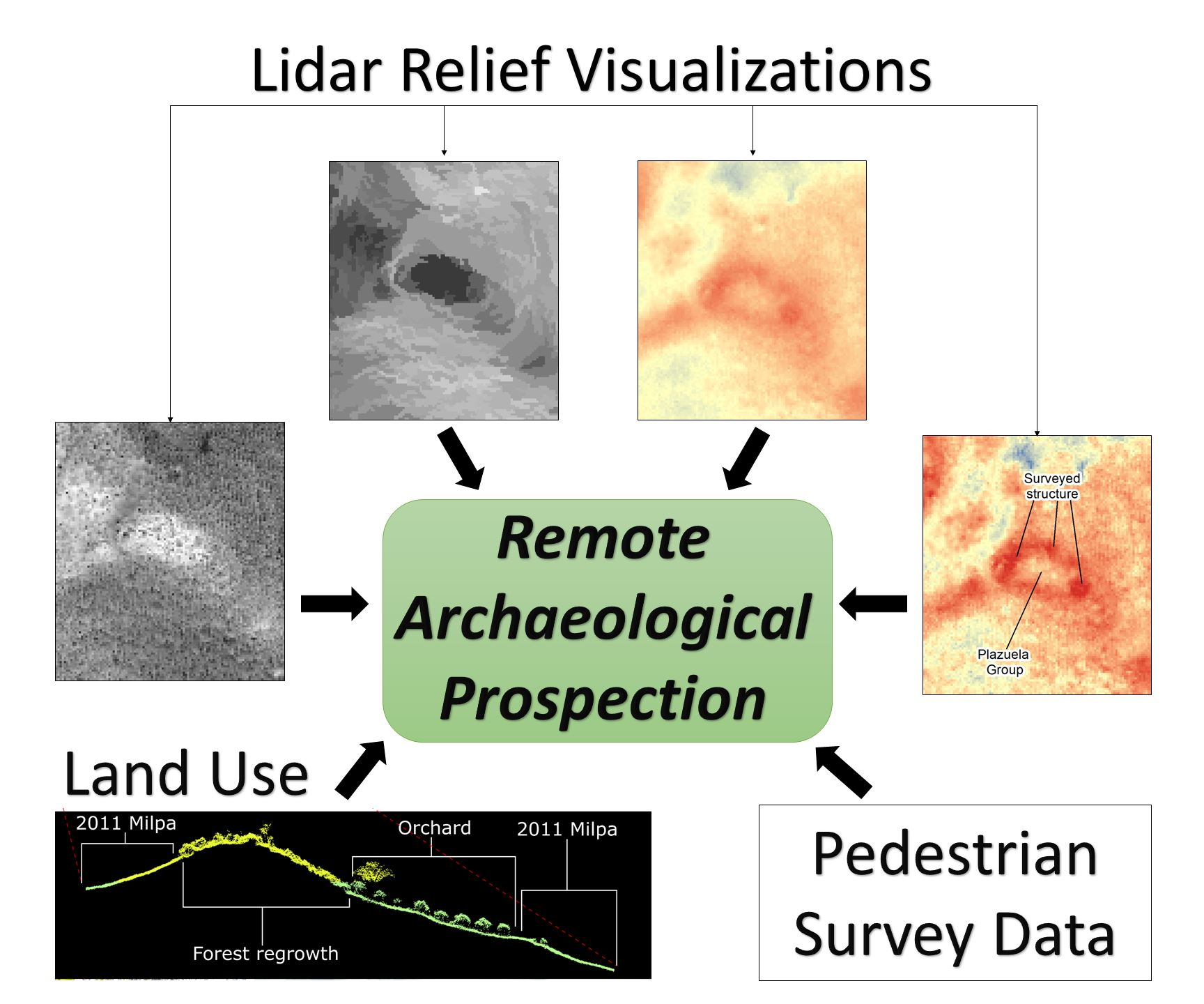
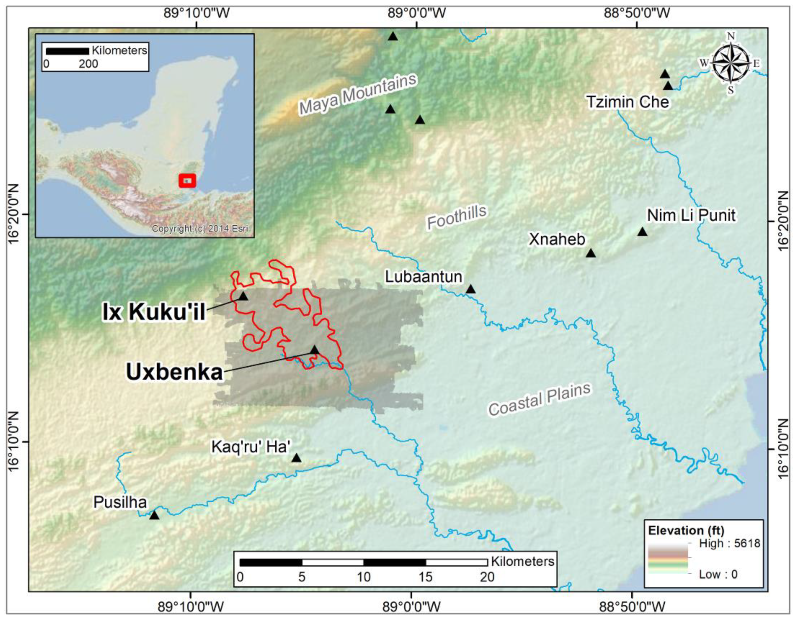
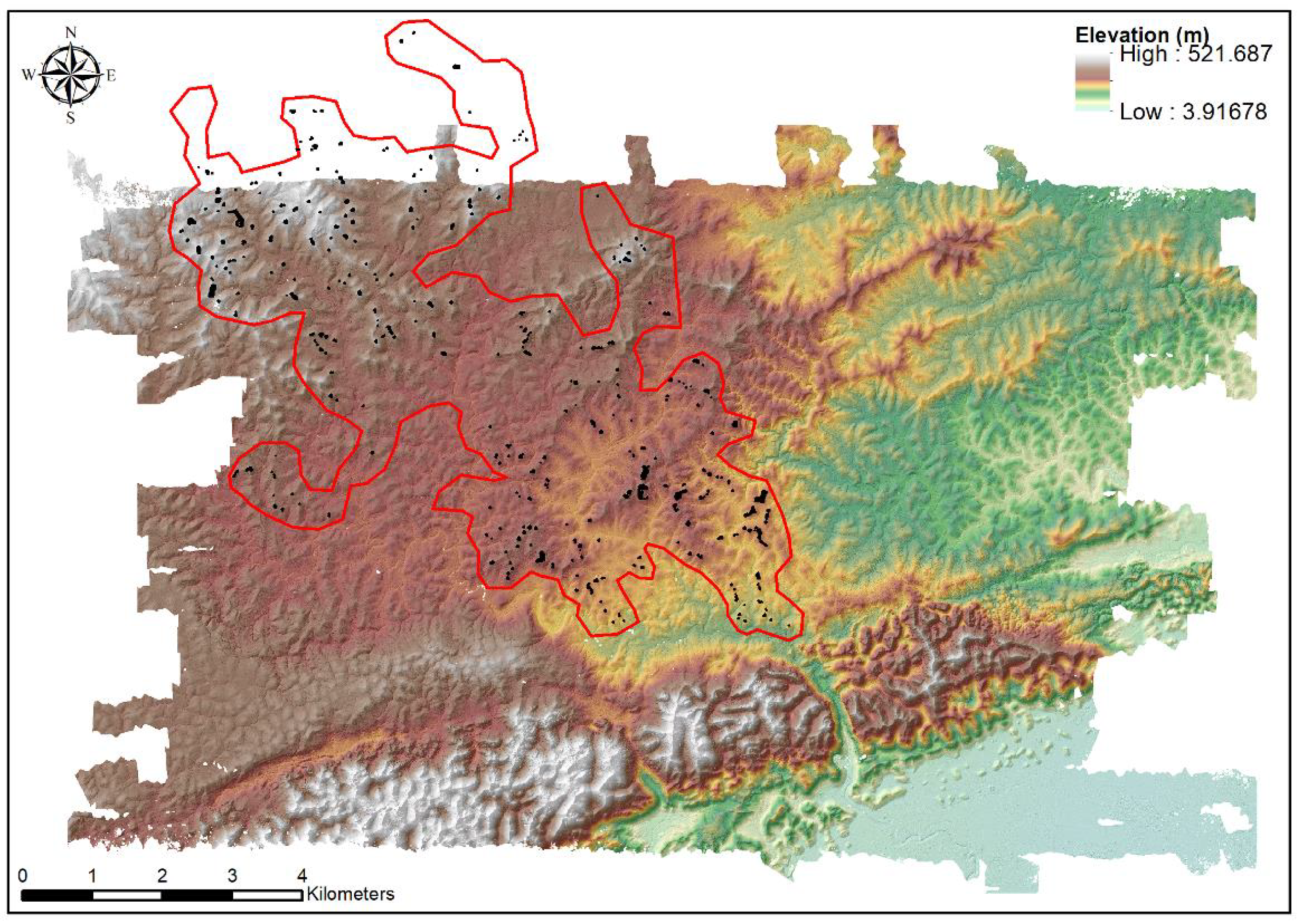
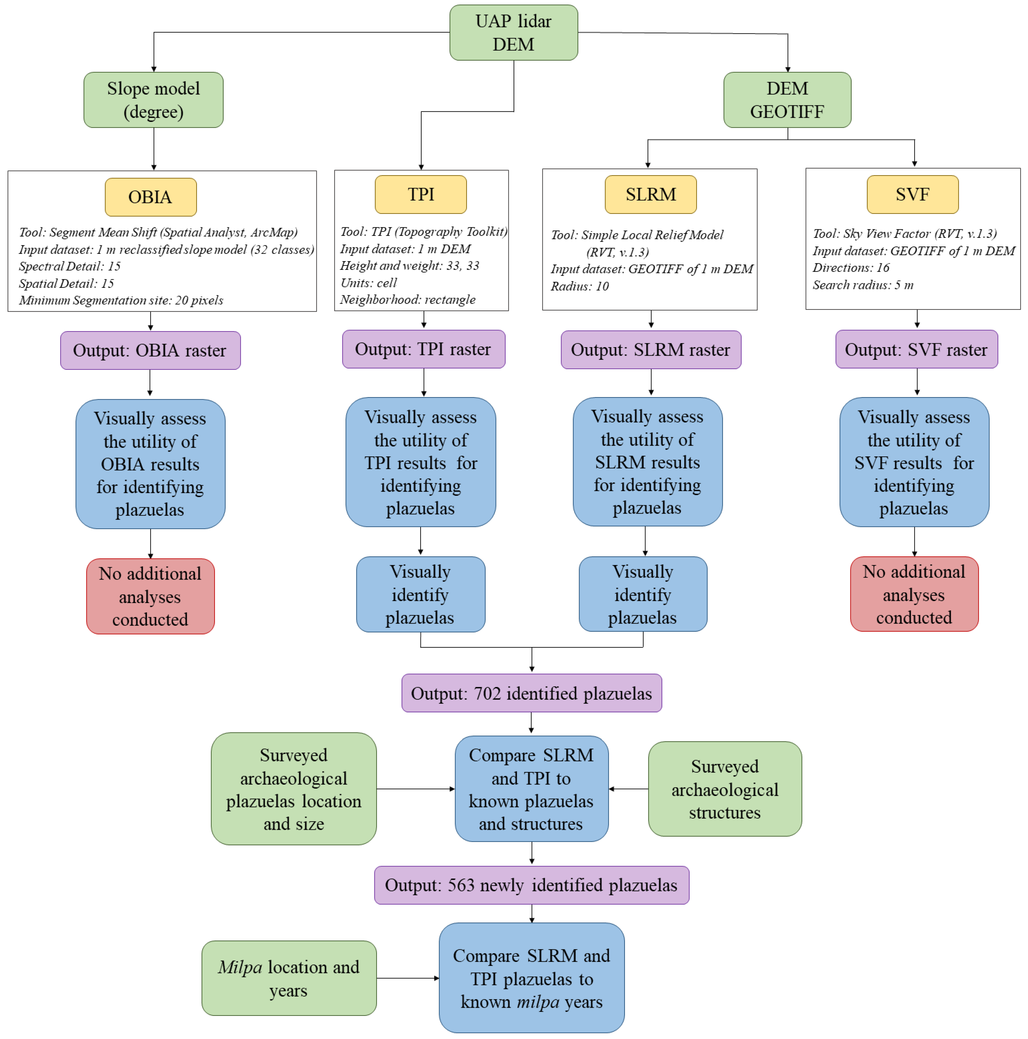
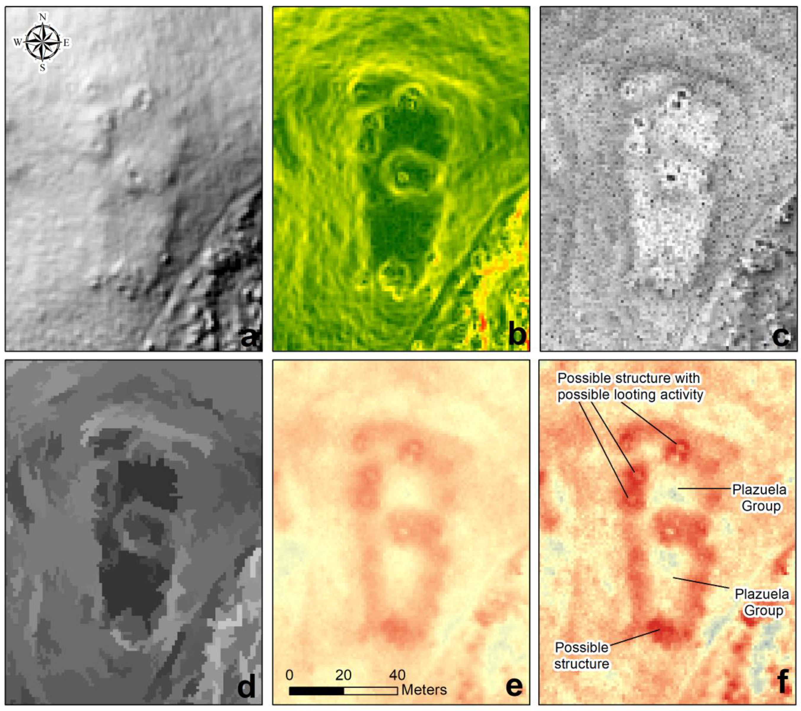
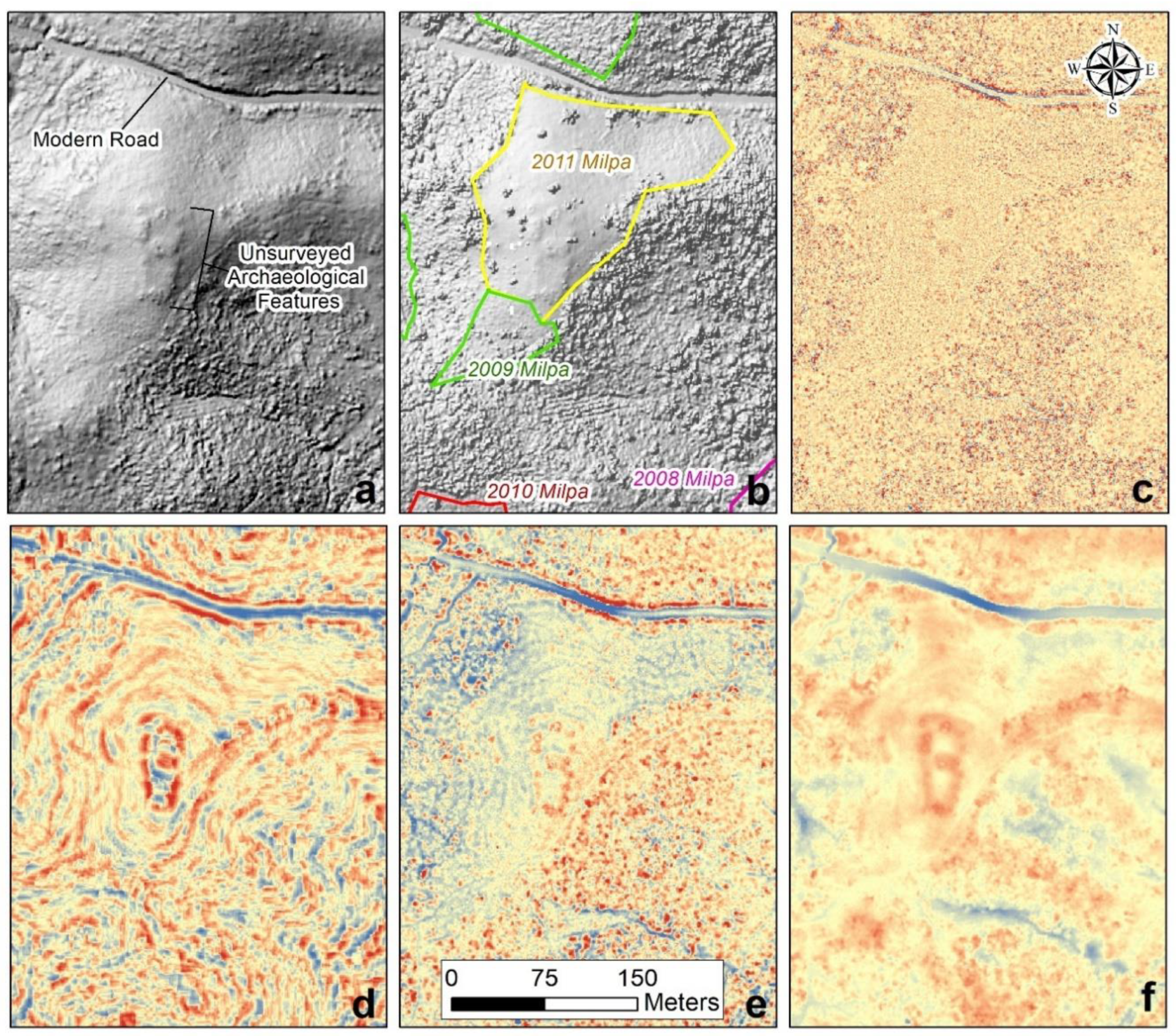
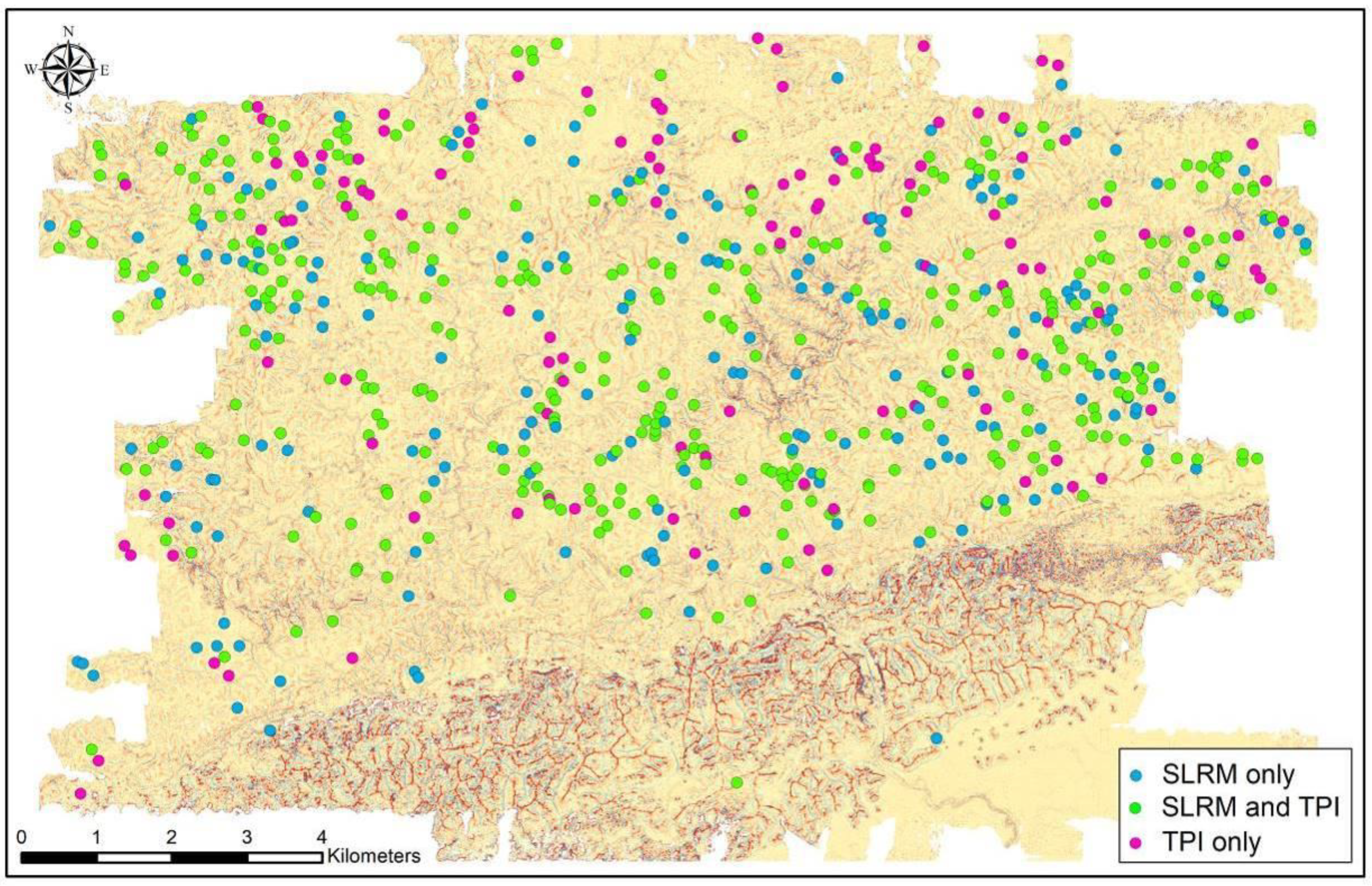
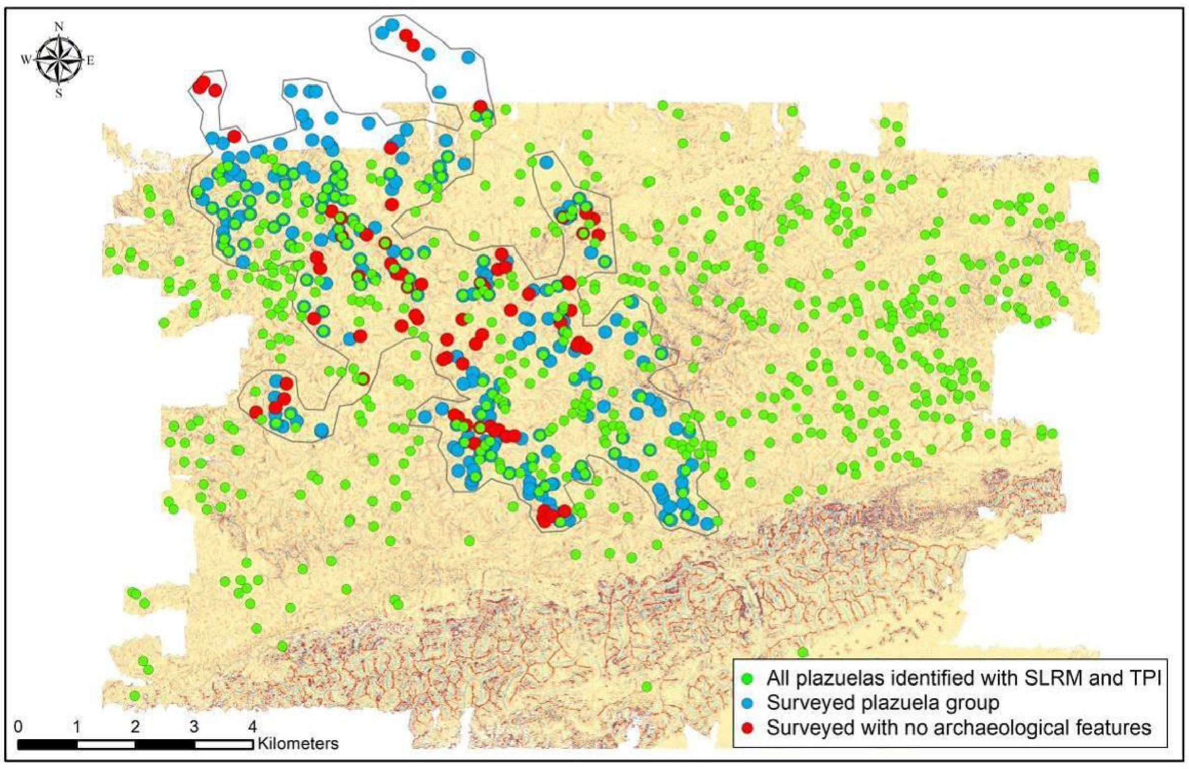
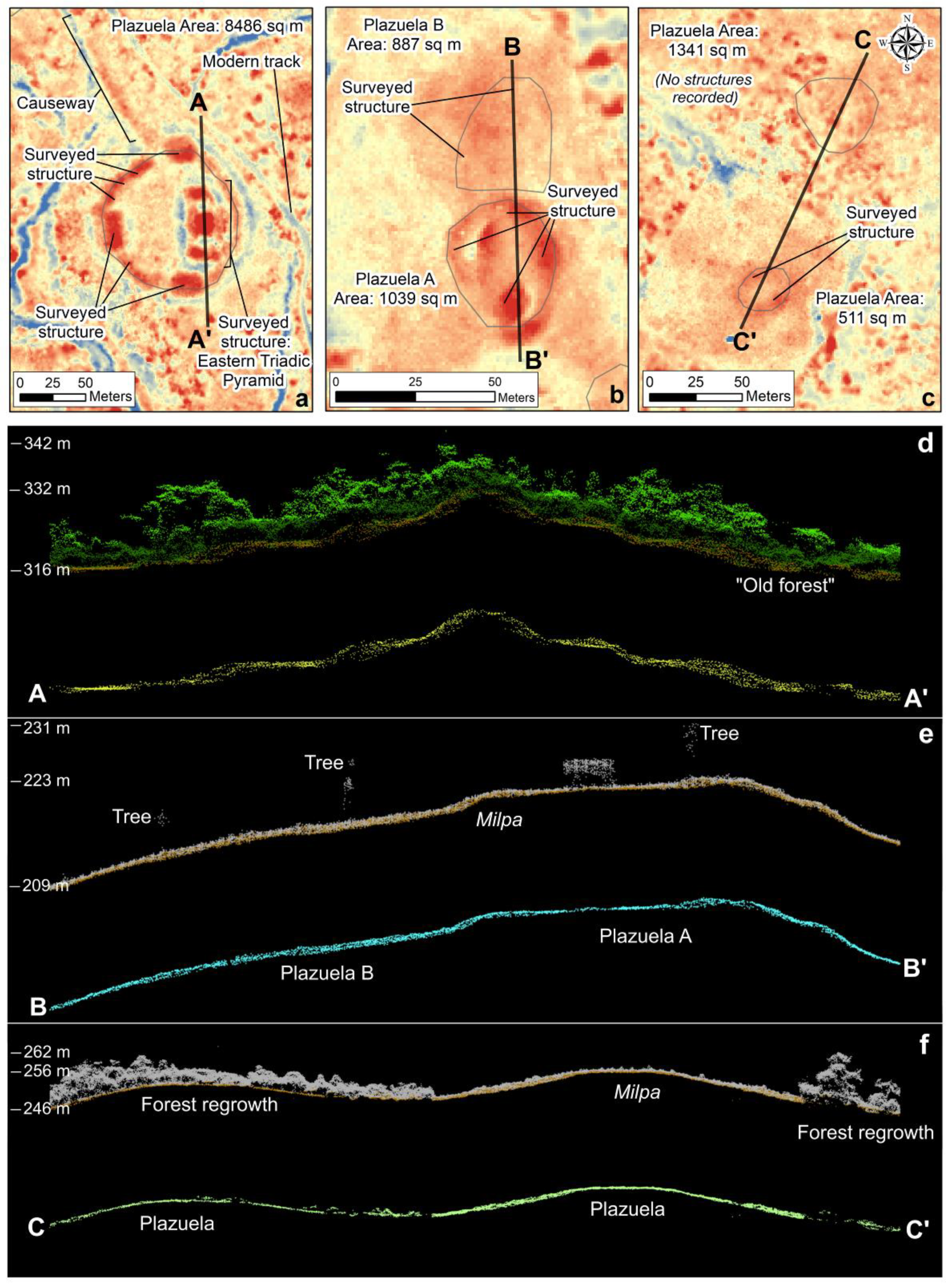
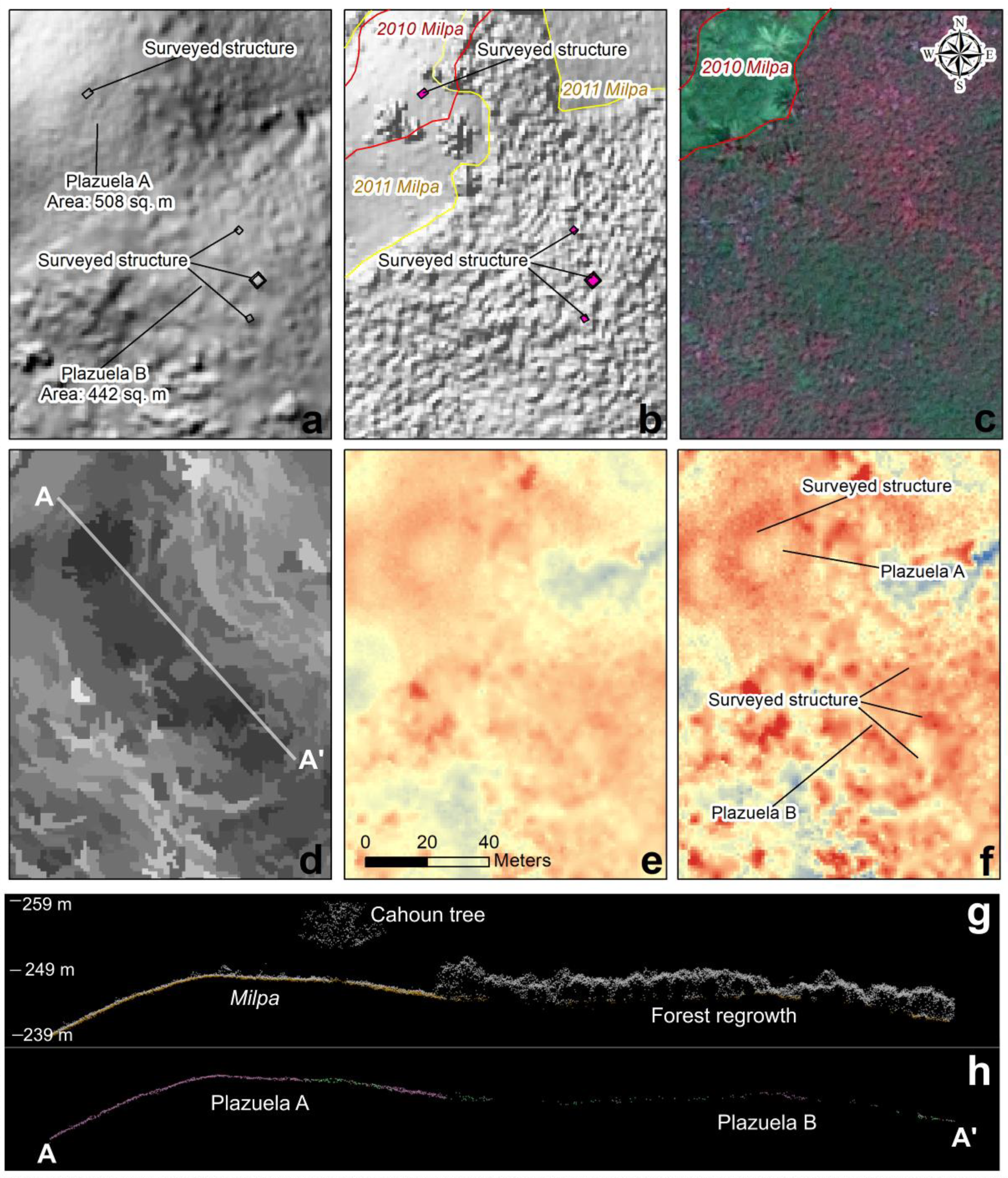
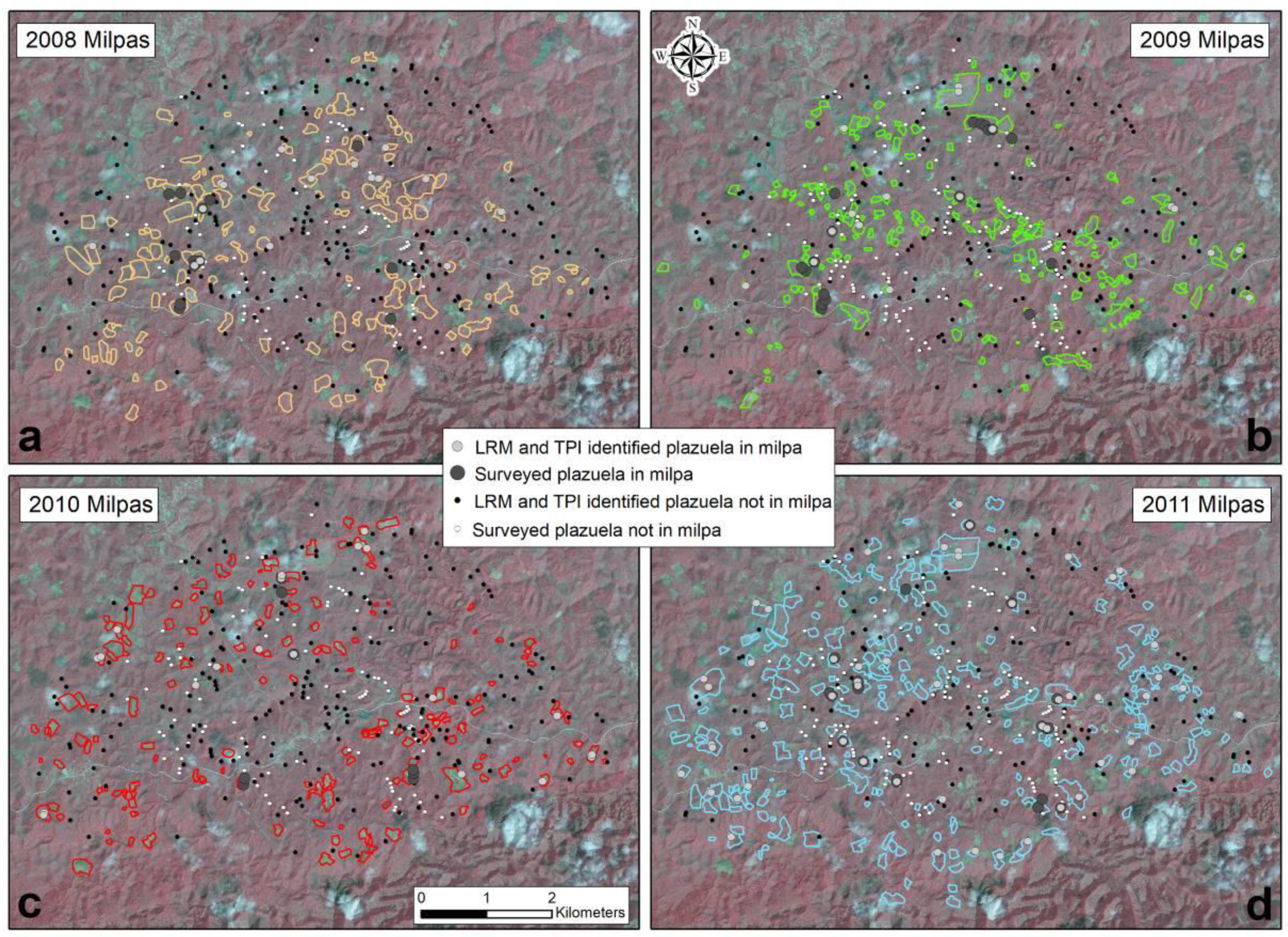
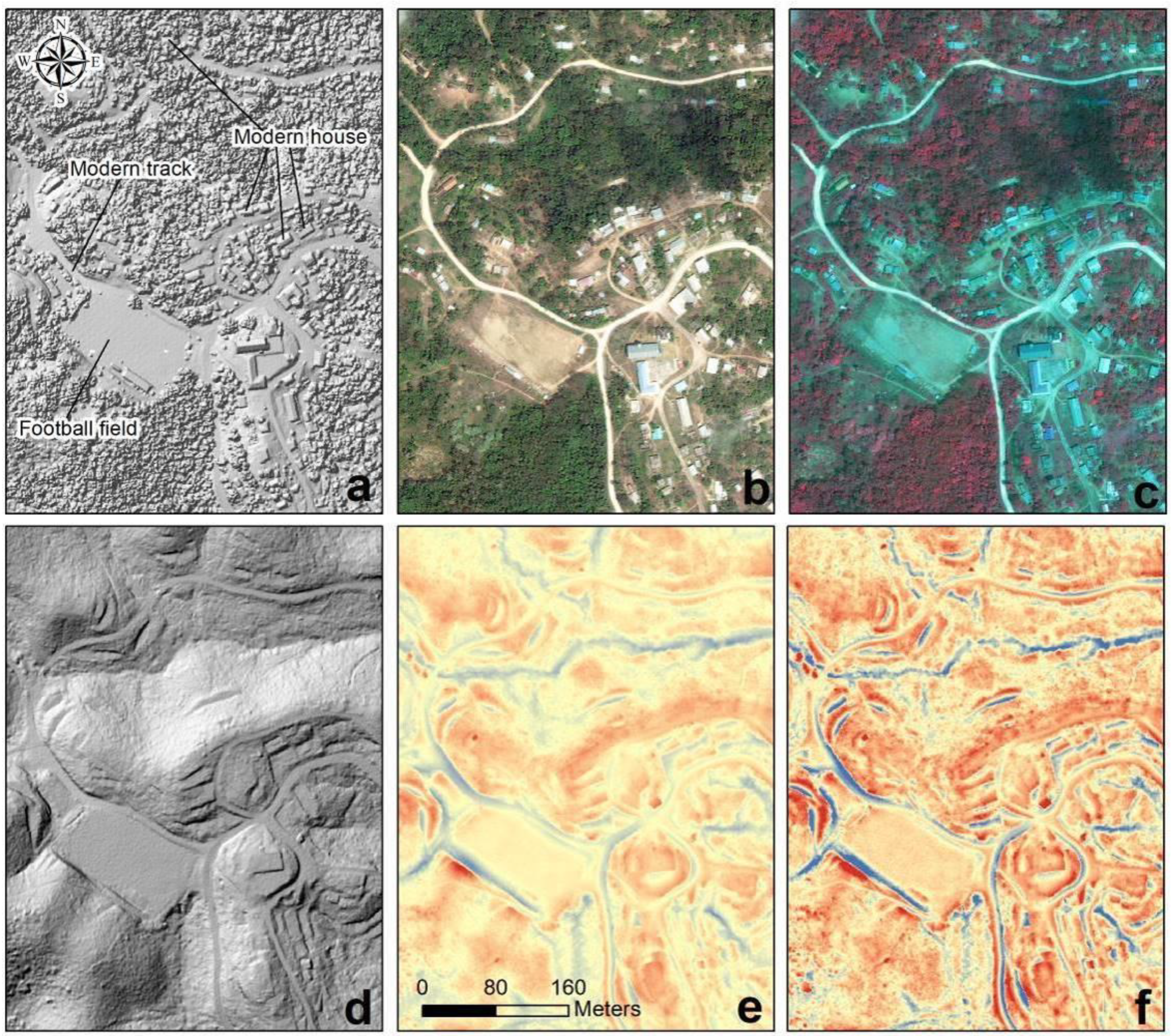
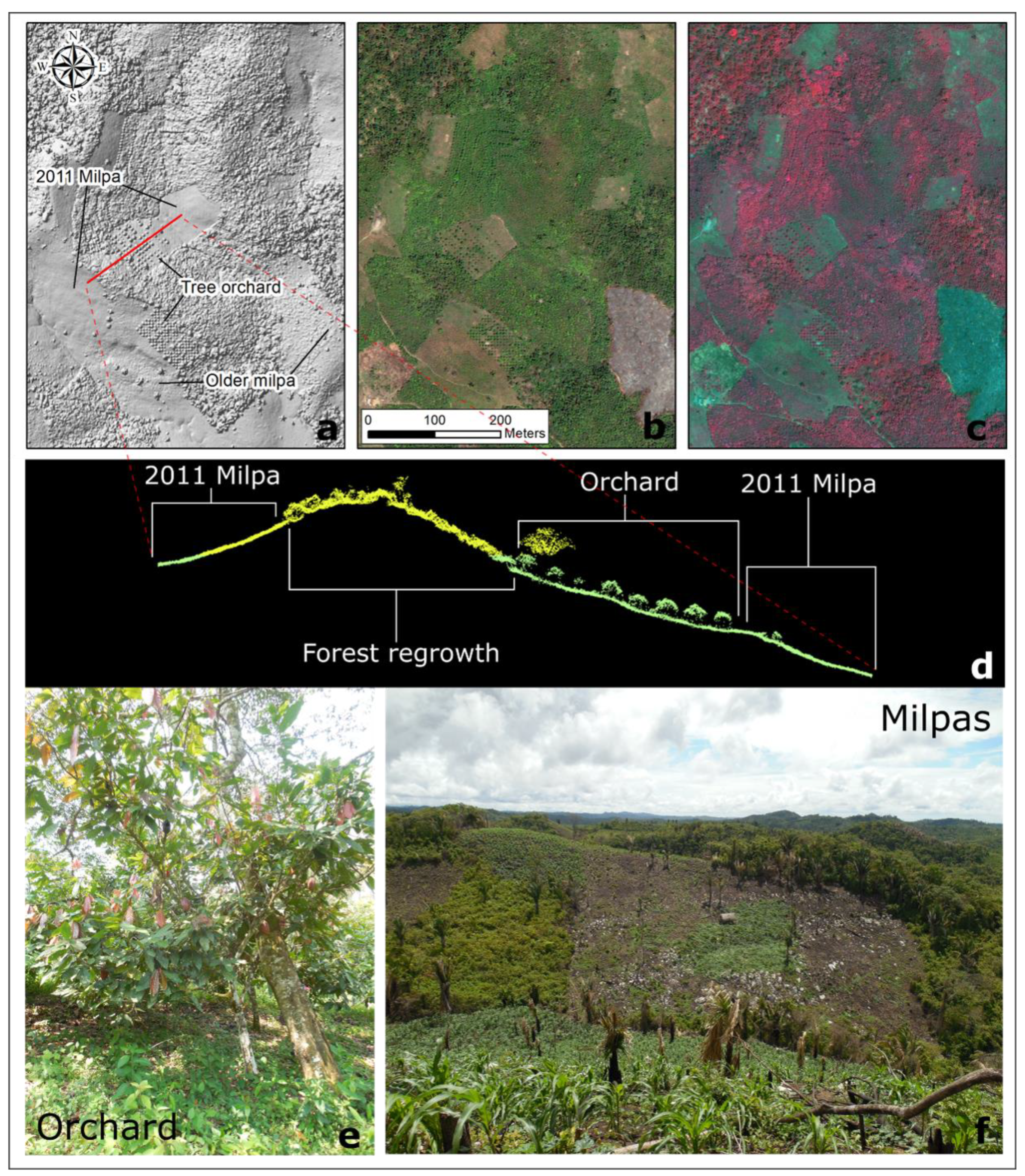
Table 1.
Comparison of plazuelas identified with SLRM and TPI.
| All TPI | All SLRM | Total all SLRM and TPI | |
|---|---|---|---|
| Total plazuelas identified | 503 | 580 | 702 |
| Number of confirmed positives (Previously surveyed plazuelas identified) | 111 | 117 | 129 |
| Number of the 315 surveyed plazuelas not identified | 204 | 198 | 186 |
| Percent of 315 surveyed plazuelas identified | 35.20% | 37.14% | 40.95% |
| Total newly identified plazuelas | 385 | 457 | 563 |
| Number of false positives (Previously documented hilltops with no archaeological features) | 7 | 6 | 10 |
| Percent of 68 previously documented hilltops with no archaeological features | 10.30% | 8.80% | 14.70% |
Table 2.
Detailed comparisons of results from only SLRM, only TPI, and both SLRM and TPI, as well as all plazuelas identified with SLRM and TPI (see Table 1).
Table 2.
Detailed comparisons of results from only SLRM, only TPI, and both SLRM and TPI, as well as all plazuelas identified with SLRM and TPI (see Table 1).
| SLRM Only | SLRM and TPI | TPI Only | All SLRM | All TPI | Total of all SLRM and TPI | |
|---|---|---|---|---|---|---|
| Plazuelas identified | 199 | 381 | 122 | 580 | 503 | 702 |
| Confirmed positives | 18 | 99 | 12 | 117 | 111 | 129 |
| Newly identified plazuelas | 178 | 279 | 106 | 457 | 385 | 563 |
| False positives | 3 | 3 | 4 | 6 | 7 | 10 |
| 2011 milpas | 14 | 39 | 1 | 53 | 40 | 54 |
| 2010 milpas | 8 | 12 | 0 | 20 | 12 | 20 |
| 2009 milpas | 6 | 9 | 2 | 15 | 11 | 17 |
| 2008 milpas | 8 | 6 | 2 | 14 | 8 | 16 |
Table 3.
Size of plazuelas and number of structures (based on pedestrian survey data) that were identified with SLRM and TPI. Larger plazuelas are more likely to be remotely identified. * Some plazuelas do not have areas calculated or number of structures recorded.
Table 3.
Size of plazuelas and number of structures (based on pedestrian survey data) that were identified with SLRM and TPI. Larger plazuelas are more likely to be remotely identified. * Some plazuelas do not have areas calculated or number of structures recorded.
| Average Area (m2) | Sample Size * | Average Number of Surveyed Structures | Sample Size * | |
|---|---|---|---|---|
| All previously surveyed plazuelas | 976.3 | 315 | 2.8 | 305 |
| SLRM only | 943.3 | 17 | 3.4 | 17 |
| SLRM and TPI | 1613.6 | 98 | 3.5 | 97 |
| TPI only | 855.6 | 12 | 3.1 | 12 |
| All SLRM | 1514.5 | 115 | 3.5 | 114 |
| All TPI | 1530.9 | 110 | 3.5 | 109 |
| Total all SLRM and TPI plazuelas | 1452.3 | 127 | 3.5 | 125 |
| All previously surveyed plazuelas (except plazuelas > 5000 sq. m) | 804.1 | 307 | - | - |
| SLRM and TPI (except plazuelas > 5000 sq. m) | 1127.4 | 91 | - | - |
| All SLRM (except plazuelas > 5000 sq. m) | 1098.4 | 108 | - | - |
| All TPI (except plazuelas > 5000 sq. m) | 1095.7 | 103 | - | - |
| Total all SLRM and TPI plazuelas except 7 largest (> 5000 sq. m) | 1074.1 | 120 | - | - |
Table 4.
Total structure counts of surveyed plazuelas compared to structure counts of plazuelas identified with SLRM and TPI. Plazuelas with more structures are more likely to be remotely identified.
Table 4.
Total structure counts of surveyed plazuelas compared to structure counts of plazuelas identified with SLRM and TPI. Plazuelas with more structures are more likely to be remotely identified.
| Number of Structures | Surveyed Plazuelas Containing the Number Structures in the First Column | SLRM and TPI Plazuelas Containing the Number Structures in the First Column | % Identified |
|---|---|---|---|
| unknown | 10 | 1 | 10% |
| 1 | 100 | 24 | 24% |
| 2 | 60 | 20 | 33% |
| 3 | 53 | 23 | 43% |
| 4 | 39 | 24 | 62% |
| 5 | 26 | 14 | 54% |
| 6 | 13 | 11 | 85% |
| 7 | 7 | 5 | 71% |
| 8 | 4 | 2 | 50% |
| 9 | 1 | 1 | 100% |
| 10 | 1 | 0 | 0% |
| 12 | 1 | 1 | 100% |
| Total plazuelas (not including unknowns) | 305 | 125 | 41% |
Table 5.
Surveyed, SLRM, and TPI plazuelas identified within milpas from 2008 to 2011 (see Reference [9]). (* Note: One SLRM and TPI plazuela identified within the milpa boundary is a false positive).
Table 5.
Surveyed, SLRM, and TPI plazuelas identified within milpas from 2008 to 2011 (see Reference [9]). (* Note: One SLRM and TPI plazuela identified within the milpa boundary is a false positive).
| milpa Year | Total in the Mapped milpa Boundary | ||||
|---|---|---|---|---|---|
| 2008 | 2009 | 2010 | 2011 | ||
| Total plazuelas through SLRM and TPI | 16 | 17 | 20 | 54 | 229 * |
| Possible plazuelas through SLRM and TPI | 13 | 12 | 18 | 41 | 165 |
| Confirmed plazuelas through SLRM and TPI | 3 | 5 | 2 | 13 | 63 |
| Confirmed plazuelas total | 13 | 18 | 8 | 20 | 171 |
| Percent of confirmed plazuelas identified with SLRM and TPI | 23.1 | 27.8 | 25.0 | 65.0 | 36.8 |
© 2020 by the author. Licensee MDPI, Basel, Switzerland. This article is an open access article distributed under the terms and conditions of the Creative Commons Attribution (CC BY) license (http://creativecommons.org/licenses/by/4.0/).
Share and Cite
MDPI and ACS Style
Thompson, A.E. Detecting Classic Maya Settlements with Lidar-Derived Relief Visualizations. Remote Sens. 2020, 12, 2838. https://doi.org/10.3390/rs12172838
AMA Style
Thompson AE. Detecting Classic Maya Settlements with Lidar-Derived Relief Visualizations. Remote Sensing. 2020; 12(17):2838. https://doi.org/10.3390/rs12172838
Chicago/Turabian StyleThompson, Amy E. 2020. "Detecting Classic Maya Settlements with Lidar-Derived Relief Visualizations" Remote Sensing 12, no. 17: 2838. https://doi.org/10.3390/rs12172838
Note that from the first issue of 2016, this journal uses article numbers instead of page numbers. See further details here.