Object-Based Multi-Temporal and Multi-Source Land Cover Mapping Leveraging Hierarchical Class Relationships

Abstract

European satellite missions Sentinel-1 (S1) and Sentinel-2 (S2) provide at high spatial resolution and high revisit time, respectively, radar and optical images that support a wide range of Earth surface monitoring tasks, such as Land Use/Land Cover mapping. A long-standing challenge in the remote sensing community is about how to efficiently exploit multiple sources of information and leverage their complementarity, in order to obtain the most out of radar and optical data. In this work, we propose to deal with land cover mapping in an object-based image analysis (OBIA) setting via a deep learning framework designed to leverage the multi-source complementarity provided by radar and optical satellite image time series (SITS). The proposed architecture is based on an extension of Recurrent Neural Network (RNN) enriched via a modified attention mechanism capable to fit the specificity of SITS data. Our framework also integrates a pretraining strategy that allows to exploit specific domain knowledge, shaped as hierarchy over the set of land cover classes, to guide the model training. Thorough experimental evaluations, involving several competitive approaches were conducted on two study sites, namely the Reunion island and a part of the Senegalese groundnut basin. Classification results, 79% of global accuracy on the Reunion island and 90% on the Senegalese site, respectively, have demonstrated the suitability of the proposal.

1. Introduction

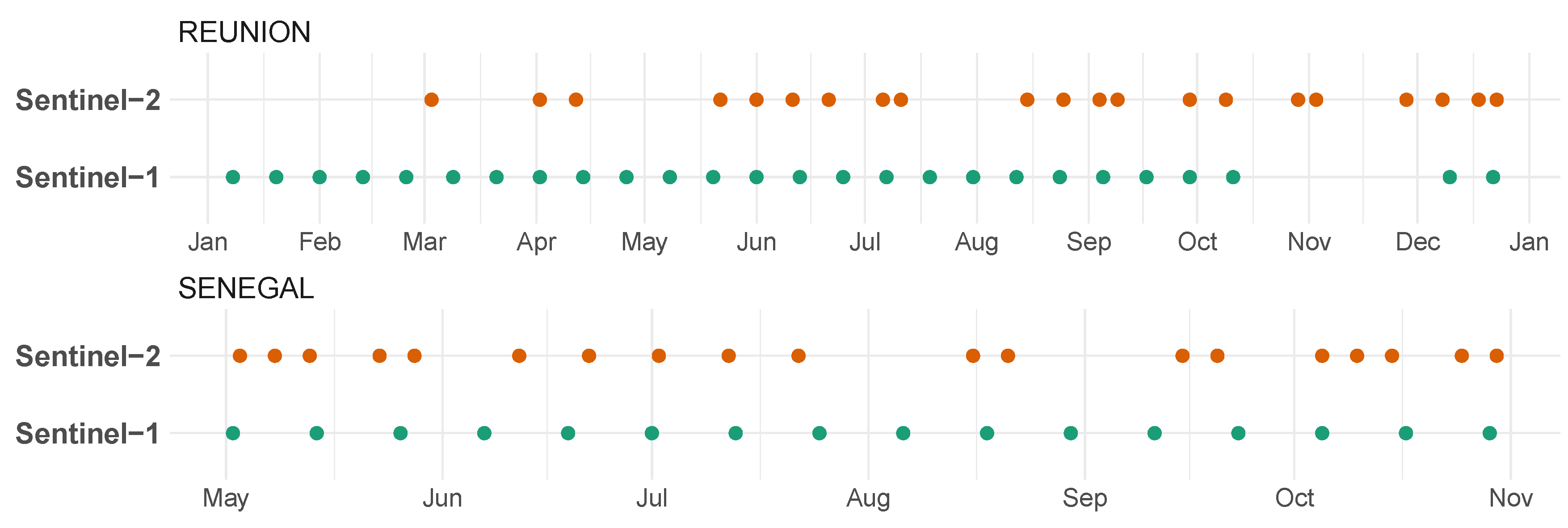
Remotely sensed data collected by modern Earth Observation systems, such as the European Sentinel programme [1], are getting increasing attention in recent years to cope with Earth surface monitoring. In particular, the Sentinel-1 and Sentinel-2 missions are of interest, since they provide publicly available multi-temporal radar and optical images respectively, with high spatial resolution (up to 10 m) and high revisit time (up to five days). Thanks to these unprecedented spatial and temporal resolutions, data coming from such sensors can be arranged in Satellite Image Time Series (SITS). SITS have been employed to deal with several tasks in multiple domains ranging from ecology [2], agriculture [3], land management planning [4], and forest and natural habitat monitoring [5,6].

Among these fields, Land Use/Land cover (LULC) mapping has received large attention in the last years [7,8,9,10], since it provides essential components on which further indicators can be built on [11]. As example, an accurate mapping of croplands and crop types is the cornerstone of agricultural monitoring systems, as it allows providing information on food production for developing countries or global market. However, cropland mapping has been identified as an important gap in agricultural monitoring systems [12].

As regards LULC mapping, both radar and optical sources have been employed, often solely, disregarding the well-known complementary existing between them, as recently underlined [13,14,15,16]. Additionally, when both sources of information are jointly used, they are independently processed without really leveraging the interplay between them, i.e., through a simple concatenation with machine learning algorithms [7,17,18] or an integration via a data fusion techniques [19,20]. In addition, such techniques ignore the spatial and temporal dependencies carried out by SITS.

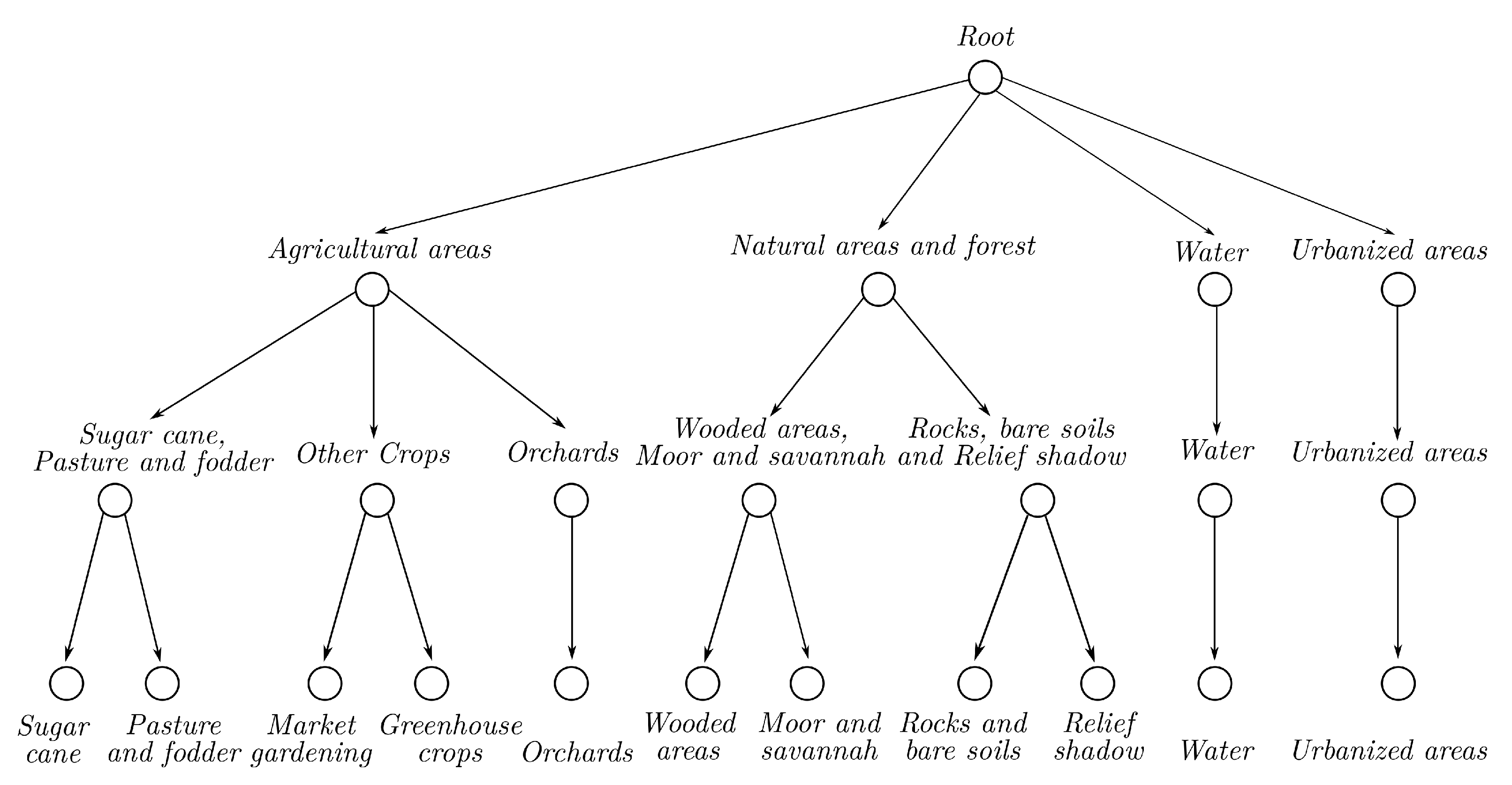
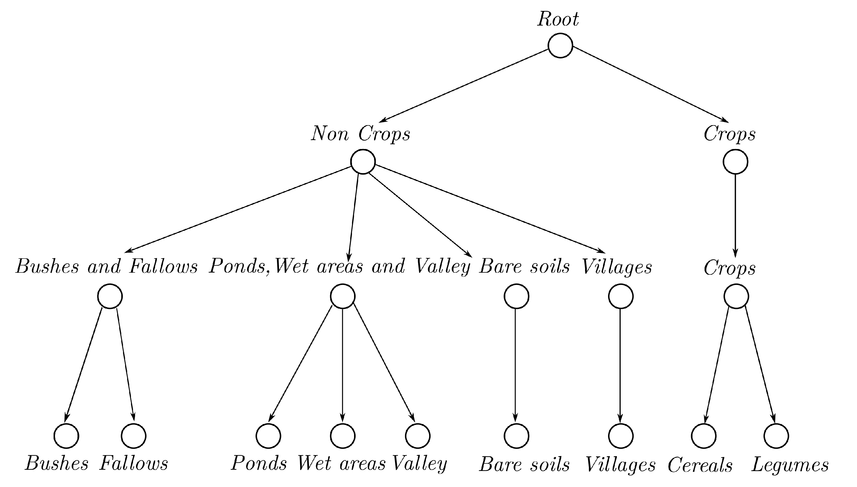
Furthermore, concerning LULC mapping domain, specific knowledge about LULC classes can be available. LULC classes can be organized hierarchically via class/subclass relationships. For instance, agricultural land cover can be organized in crop types and subsequently crop types in specific crops. A notable example of such hierarchical organization is the Food and Agriculture Organization (FAO)–Land Cover Classification System (LCCS) [21]. Because of the presence of such class/subclass relationships, most of the time, we can derive a hierarchical or taxonomic organization of LULC classes that could be appealing to consider in subsequent land cover mapping process. Only few studies, today, have considered the use of such hierarchical information to deal with land cover mapping [22,23,24]. Generally, such frameworks build an independent classification model for each level of the hierarchy and the decision made at a certain level of the taxonomy cannot be modified, further, in the decision process.

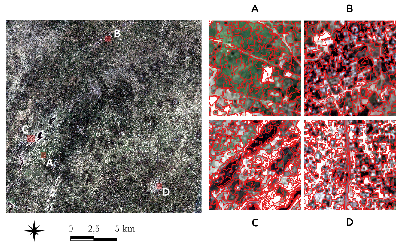
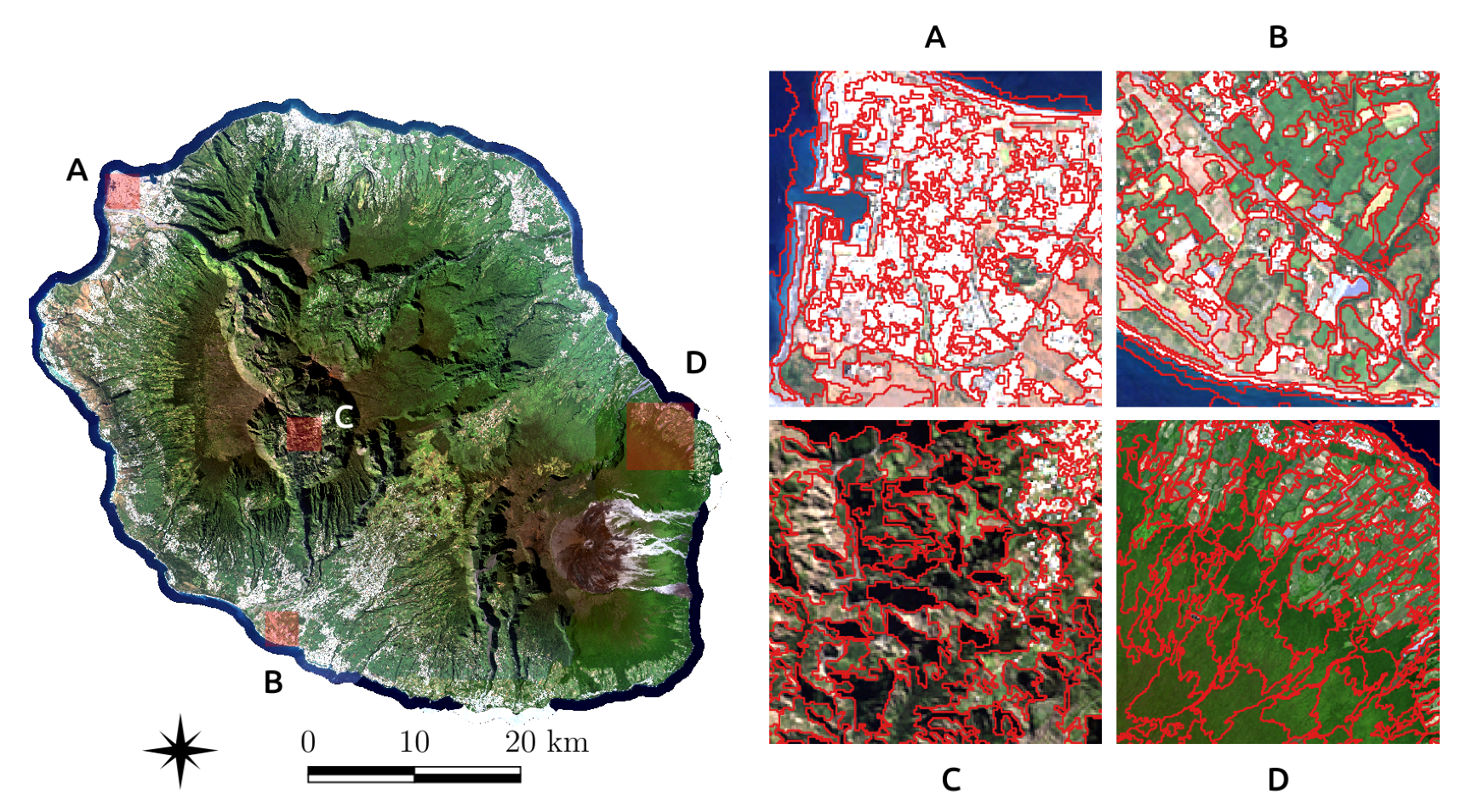
Another challenge to deal with when carrying out land cover mapping is related to the spatial granularity at which the remote sensing time series data are analysed: pixel or object [25]. While in the pixel based analysis, the basic units are the pixels, in object-based image analysis (OBIA), the images are first segmented obtaining groups of radiometrically homogeneous pixels: the objects, which become the basic units in any further analysis. Considering objects instead of pixels has the main advantage to work with more coherent piece of information that are simpler to interpret [26] for an end user or field expert.

Nowadays, Deep Learning (DL) is pervasive in many domains including remote sensing [27,28,29,30]. When considering the use of multi-source (radar and optical) data in the context of LULC mapping, authors in [3] employed a Convolutional Neural Network (CNN) based architecture to combine Sentinel-1 and Landsat-8 images for land cover and crop types mapping. This CNN architecture processed the data with convolutions in both spatial and spectral domains while the temporal domain was not taken into account. Authors in [14] proposed the TWINNS architecture, a combination of CNN and Convolutional Recurrent Neural Network [31] (ConvRNN) aiming to leverage both spatial and temporal dependencies in the SITS data as well as the complementarity of radar and optical sensors. Such approaches work at pixel level and do not exploit additional background information (i.e., class/subclass relationships) during their learning process. Furthermore they are not directly transferable to object-level analysis as it is. Recently, authors in [15] proposes a preliminary investigation of Recurrent Neural Network (RNN) approaches introducing the OD2RNN model for multi-source land cover mapping. Recurrent Neural Networks are exploited to deal with SITS in an OBIA framework instead of ConvRNN, since the latter cannot be applied to the agglomerate statistics describing the object-level SITS.

We introduce in this work the DL-based HOb2sRNN (Hierarchical Object based two-Stream Recurrent Neural Network) architecture in order to deal with land cover mapping at object level using multi-source (radar and optical) SITS data and exploiting hierarchical relationships among land cover classes. Our framework is tailored for a common OBIA setting, where a prior segmentation is typically performed to provide a suitable object layer, and the so-obtained segments are attributed using agglomerate statistics starting from the available image set, to be subsequently used as samples for training and classification. HOb2sRNN is therefore conceived to perform object-based LULC mapping given the radar and optical object SITS available on the study area, the relative ground truth data and the associated land cover class hierarchy. Building upon the preliminary work presented in [15], as a major further contribution, here, we propose an architecture that is based on an extended RNN model enriched via a modified attention mechanism capable of fitting the specificity of SITS data. In addition, we also introduce a pretraining strategy to get the most out of the information available under the shape of hierarchical relationships between land cover classes. Last but not least important, differently from previous works on multi-source and multi-temporal land cover mapping that exploits DL methods [14,15], we also provide, in this study, a contribution related to the interpretability of the proposed model. More specifically, we investigate and discuss how the side information provided by HOb2sRNN can be leveraged to draw some connections between the way in which the model takes its decision and the agronomic knowledge we have.

With the aim to provide an in-depth assessment of the HOb2sRNN behaviour, an extensive experimental evaluation is conducted on two study sites with diverse land cover characteristics, namely the Reunion island and a part of the Senegalese groundnut basin, the latter being dominated by small scale agriculture and limited in the amount of available data. The results have underlined the effectiveness of our proposal when compared to competitive and recent approaches commonly leveraged to deal with land cover mapping task, including the work presented in [15].

The remainder of this work is structured, as follows: first, the study sites and associated data are introduced in Section 2; and then Section 3 describes the proposed method while the experimental settings and the evaluations are carried out and discussed in Section 4 and Section 5, respectively, and finally, Section 6 draws the conclusion.

2. Materials

The analysis was carried out on 2 study sites characterized by different landscapes and land cover classes: the Reunion island, a French overseas department located in the Indian Ocean and a part of the Senegalese groundnut basin located in central Senegal. The Reunion island covers an area of a little over 3000 km${}^2$, while the Senegalese site area is about 500 km${}^2$. The former benchmark involves 26 Sentinel-1 (S1) and 21 Sentinel-2 (S2) satellite images acquired during the year 2017 while the latter consists of 16–S1 and 19–S2 images collected between May and October 2018 (see Figure 1 for acquisition date details).

2.1. Sentinel-1 Data

The radar images were acquired in C-band Interferometric Wide Swath (IW) mode with dual polarization (VH and VV) and in ascending orbit. All images as retrieved at level-1C Ground Range Detected (GRD) from the PEPS platform (https://peps.cnes.fr/) were first radiometrically calibrated in backscatter values (decibels, dB) using parameters that were included in the metadata file, then coregistered with the Sentinel-2 grid and orthorectified at the same 10-m spatial resolution. Finally, multi-temporal filtering was applied to the time series in order to reduce the speckle effect.

2.2. Sentinel-2 Data

The optical images were downloaded from the THEIA pole platform (http://theia.cnes.fr) at level-2A top of canopy reflectance. Only 10-m spatial resolution bands (i.e., Blue, Green, Red and Near Infrared spectrum) containing less than 50% of cloudy pixels were considered in this analysis. A preprocessing was performed over each band to replace cloudy observations as detected by the supplied cloud masks through a multi-temporal gapfilling [4]. Cloudy pixel values were linearly interpolated using the previous and following cloud-free dates. Finally, the Normalized Difference Vegetation Index (NDVI) [32] was calculated for each date. NDVI was considered as supplementary optical descriptor since it captures well the vegetation activity which is subject to change over time.

2.3. Ground Truth

Considering the Reunion island (Reunion island land cover dataset is available online on the CIRAD dataverse under doi:10.18167/DVN1/TOARDN), the ground truth (GT) was built from various sources: the Registre Parcellaire Graphique (RPG) (RPG is part of the European Land Parcel Identification System (LPIS), provided by the French Agency for services and payment) reference data for 2014, GPS land cover records from June 2017 and the visual interpretation of very high spatial resolution (VHSR) SPOT6/7 images (1.5-m) completed by a field expert with knowledge of territory. Additional information about this dataset can be found in [33]. As regards the Senegalese site, the ground truth was built from GPS land cover records that were collected during the 2018 field campaign with the same approach as for the Reunion site followed by a visual interpretation of a VHSR PlanetScope image (3-m). Both operations were conducted by a specialist of the study area. For each site, the GT was assembled in Geographic Information System vector file, containing a collection of polygons each attributed with the corresponding land cover class. The Reunion island GT includes 6265 polygons that were distributed over 11 classes while the Senegalese site includes 734 polygons distributed over nine classes (See

Table 1. Characteristics of the Reunion island ground truth.

Class	Label	Polygons	Segments
0	Sugarcane	869	1258
1	Pasture and fodder	582	869
2	Market gardening	758	912
3	Greenhouse crops or shadows	260	233
4	Orchards	767	1014
5	Wooded areas	570	1106
6	Moor and Savannah	506	850
7	Rocks and natural bare soil	299	573
8	Relief shadows	81	107
9	Water	177	261
10	Urbanized areas	1396	725
Total		6265	7908

and

Table 2. Characteristics of the Senegalese site ground truth.

Class	Label	Polygons	Segments
0	Bushes	50	100
1	Fallows and Uncultivated areas	69	322
2	Ponds	33	59
3	Banks and bare soils	35	132
4	Villages	21	767
5	Wet areas	22	156
6	Valley	22	56
7	Cereals	260	816
8	Legumes	222	676
Total		734	3084

).

In order to inject specific knowledge in the learning process, we obtained from field experts, for each study site, a taxonomy of land cover classes (See Figure 2 and Figure 3), getting two levels of representation before the target classification level described in Table 1 and Table 2.

To analyse data at object-level, a segmentation was performed for each study site in close collaboration with the field experts to provide a convenient object layer. To this end, we used the VHSR images at hand (i.e., SPOT6/7 and PlanetScope) which have been coregistered with the corresponding Sentinel-2 grid to ensure a precise spatial matching. The VHSR images were segmented using the Large Scale Generic Region Merging (LSGRM) module in the Orfeo Toolbox [34] obtaining 14,465 segments on the Reunion island and 116,937 segments on the Senegalese site, respectively. The segmentation algorithm parameters were adjusted by visual interpretation via several trial processes, so that the final obtained segments fit as closely as possible land cover units of the study sites. Figure 4 and Figure 5 show some details about the segmentation outcomes. Subsequently, for each study site, the GT polygons were spatially intersected with the obtained segments to provide radiometrically homogeneous class samples. This process resulted in new labeled segments of comparable size: 7908 for the Reunion island and 3084 segments for the Senegalese site (see Table 1 and Table 2). Finally, the average pixel values corresponding to each of these segments were extracted over the time series, giving 157 features per segment (26 time stamps × two bands for S1 + 21 time stamps × five bands for S2) for classification on the Reunion island and 127 features per segment (16 time stamps × two bands for S1 + 19 time stamps × five bands for S2) for classification on the Senegalese site.

3. Method

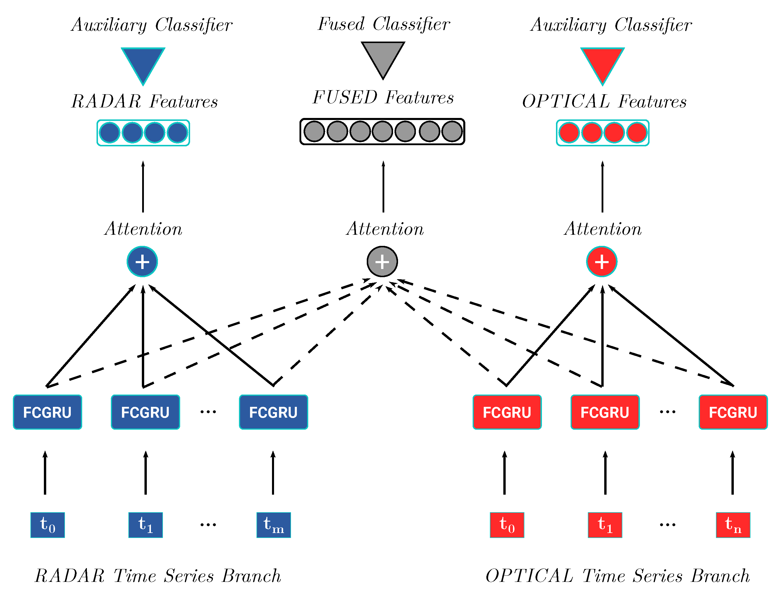
Figure 6 depicts the proposed deep learning architecture, named HOb2sRNN, for the multi-source SITS classification process. The architecture involves two branches: one for the radar SITS (left) and one for the optical SITS (right). At the end of the per-source analysis, the results of the two branches are merged and a final decision is made. The model automatically combines the multi-source and multi-temporal information in an end-to-end process. The output of the model is a land cover classification for each pair of time series (radar and optical). Each branch of the HOb2sRNN architecture can be decomposed in two parts: (i) the time series analysis through the extended Gated Recurrent Unit cell, we named FCGRU and (ii) the multi-temporal combination to generate per-source features employing a modified attention mechanism. Moreover, the per branch FCGRU outputs are concatenated and the attention mechanism is employed again to extract fused features. Finally, the extracted per branch and fused features are leveraged to produce the final land cover classification. Such learned features, named $fea{t}_{rad}$, $fea{t}_{opt}$, and $fea{t}_{fused}$, indicate, respectively, the output of the radar branch, the optical branch, and the source fusion. In addition, the architecture is trained leveraging domain knowledge represented under the shape of hierarchy that organizes land cover classes in a taxonomy with class/subclass relationships. The hierarchical information is exploited to pretrain the HOb2sRNN architecture considering tasks of increasing complexity. Section 3.4 details the process.

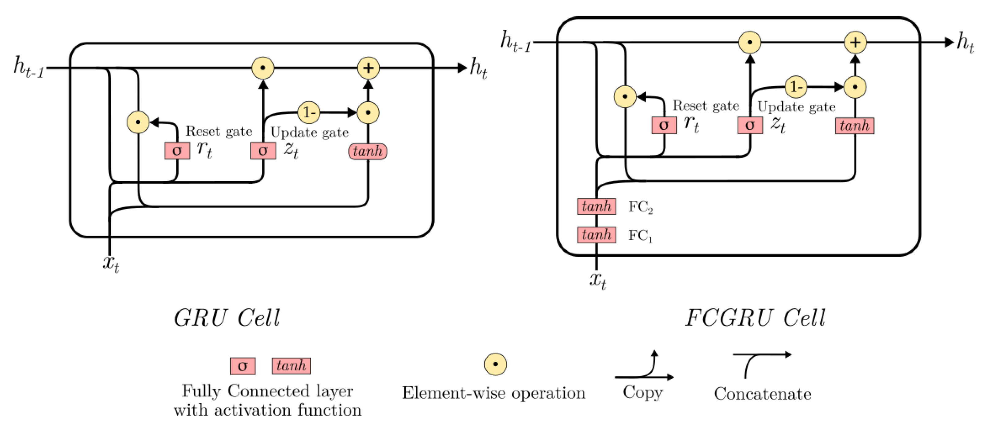
3.1. Fully Connected Gated Recurrent Unit (FCGRU)

The first part of each branch is constituted by an enriched Gated Recurrent Unit that extends standard GRU [35]. We name such enriched GRU as Fully Connected GRU (FCGRU). In Figure 7 we illustrate the standard GRU unit and the introduced FCGRU. The FCGRU cell extends the GRU unit by involving two fully connected layers namely $F{C}_1$ and $F{C}_2$ at the beginning of the cell pipeline. Such layers preprocess the input time series information before starting the standard GRU unit transformation. Therefore, they allow for the architecture to extract an useful input combination for the classification task, enriching the original representation of the object time series. More specifically, $F{C}_1$ takes as input the object time series (radar or optical) and its output is used to feed $F{C}_2$. A Hyperbolic Tangent ($tanh$) non-linearity is associated to each of the fully connected layers for the sake of consistency with the GRU unit that is mainly based on Sigmoid and $tanh$ functions. The $tanh$ activation function has an S-shape and is delimited in the range [$-1,1$]. Successively, the standard GRU unit transformation is employed over the enriched representation (output of $F{C}_2$). It is composed of a hidden state $h_{t-1}$, the reset gate $r_t$, and the update gate $z_t$. The gates regulate the information to be forgotten or remembered during the learning process and deal with the vanishing and exploding gradient problem. The output of the unit is the new hidden state $h_t$. Dropout was employed in the FCGRU cell on the ongoing states and between the two fully connected layers to prevent overfitting. The following equations formally describe the extended GRU cell:

$$x_{t^{\prime }}=tanh(W_{2}tanh(W_1{x}_t+b_1)+b_2)$$

(1)

$$z_t=\sigma (W_{zx}{x}_{t^{\prime }}+W_{zh}{h}_{t-1}+b_z)$$

(2)

$$r_t=\sigma (W_{rx}{x}_{t^{\prime }}+W_{rh}{h}_{t-1}+b_r)$$

(3)

$$h_t=z_t\odot h_{t-1}+(1-z_t)\odot tanh(W_{hx}{x}_t+W_{hr}(r_t\odot h_{t-1})+b_h)$$

(4)

The ⊙ symbol indicates an element-wise multiplication while $\sigma$ and tanh represent Sigmoid and Hyperbolic Tangent function, respectively. $x_t$ is the time stamp input vector and $x_{t^{\prime }}$ is the enriched input vector representation. The different weight matrices $W_{*}$, $W_{**}$, and bias vectors $b_{*}$ are the parameters learned during the training of the model.

3.2. Modified Attention Mechanism

The second part of the branches consists of a modified neural attention mechanism on top of the output hidden states produced by the FCGRU cell. Attention strategies [36,37,38] are widely used in one-dimensional (1D) signal or natural language processing to combine RNN outputs at different time stamps through a set of attention weights. In the traditional attention mechanism, the set of weights is computed using a $SoftMax$ function so that their values ranges in [$0,1$] and their sum is equal to 1 providing at the same time a probabilistic interpretation. Due to the sum constraint, the $SoftMax$ attention has the property to prioritize one instance over the others making it well suited for tasks such as machine translation where each target word is aligned to one of the source word [39]. However, in the remote sensing time series classification context, forcing the sum of weights to 1 may not be fully beneficial for the attention model. In fact, considering a specific time series classification task where almost all of the time stamps are relevant for the problem, the use of a SoftMax function to compute attention weights will squash towards zero the attention weights since their sum should be one and finally the attention combination may not be efficient as expected. Therefore, relaxing this constraint could help the model to better weight the relevant time stamps independently. In our attention formulation, we attempted to address this point by substituting the $SoftMax$ function with a Hyperbolic Tangent to compute attention weights. The motivation behind the $tanh$ attention, in addition to the sum constraint relaxation, is that the learned attention weights will be in a wider range i.e., [$-1,1$], also allowing negative values. The equations below describe the $tanh$ attention formulation that we introduced:

$$score=tanh(H·W+b)·u$$

(5)

$$\lambda =tanh\left(score\right)$$

(6)

$$feat=\sum _{i=1}^N{\lambda }_i{h}_{t_i}$$

(7)

where $H\in {\mathbb{R}}^{N,d}$ is a matrix obtained by vertically stacking all hidden state vectors $h_{t_i}\in {\mathbb{R}}^d$ learned at the N different time stamps by the FCGRU; $\lambda \in {\mathbb{R}}^d$ is the attention weight vector traditionally computed by a $SoftMax$ function that we replaced by a $tanh$ function; matrix $W\in {\mathbb{R}}^{d,d}$ and vectors $b,u\in {\mathbb{R}}^d$ are parameters learned during the process.

The described attention mechanism is employed over the FCGRU outputs (hidden states) in the radar and optical branches to generate per-source features ($fea{t}_{rad}$ and $fea{t}_{opt}$). Such features encode the temporal information related to the input sources. Furthermore, the per-source hidden states are concatenated and an additional attention mechanism is employed over them to generate fused features ($fea{t}_{fused}$). Such features encode both temporal information and complementarity of radar and optical SITS. Thus, the architecture involves learning three sets of attention weights: ${\lambda }_{rad}$, ${\lambda }_{opt}$ and ${\lambda }_{fused}$, which refers, respectively, to the attention mechanisms employed over the radar, optical and concatenated hidden states.

3.3. Feature Combination

Once each set of features has been yielded, they are directly leveraged to perform the final land cover classification. The combination process involves three classifiers: one main classifier on top of the fused features and two auxiliary classifiers, one for each source features. The main classifier is composed of two fully connected layers and a $SoftMax$ layer. The fully connected layers are associated to a ReLU non linearity and followed by a dropout layer each. The auxiliary classifiers are composed of one $SoftMax$ layer each. Auxiliary classifiers [10,14,40] are used to strengthen the complementarity as well as the discriminative power of the per-source learned features. 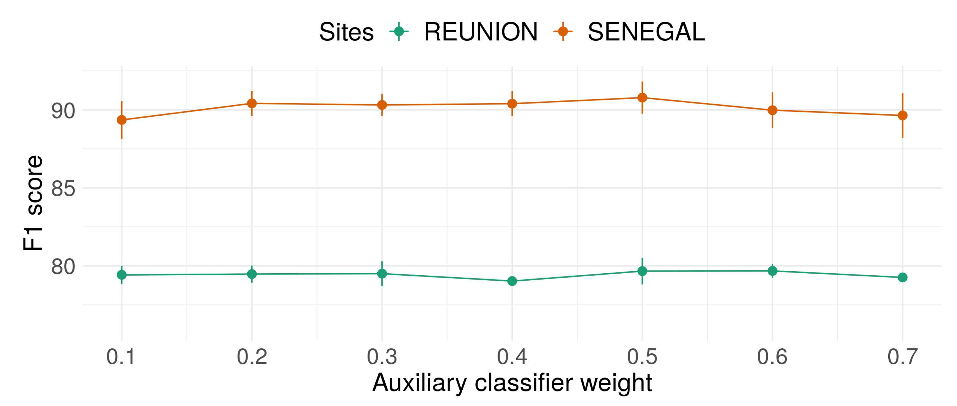Their goal is to stress the fact that the learned features need to be discriminative alone i.e., independently from each other [10,14,41]. Subsequently, the cost function associated to the optimization of the three classifiers is:

$$L_{total}=L\left(fea{t}_{fused}\right)+\alpha \sum _{source\in \{rad,opt\}}L\left(fea{t}_{source}\right)$$

(8)

where $L\left(feat\right)$ is the loss computed by the categorical Cross-Entropy function and associated to the classifier fed with the features $feat$. The contribution of the auxiliary classifiers is weighted by the parameter $\alpha$. The final land cover class is obtained by combining the three classifier outcomes with the same weighting schema employed in the loss computation:

$$score=scor{e}_{fused}+\alpha \sum _{source\in \{rad,opt\}}scor{e}_{source}$$

(9)

where $scor{e}_{fused}$ and $scor{e}_{source}$ are respectively the prediction scores of the fused classifier and the auxiliary classifier associated to one of the radar or optical branch. We empirically set the value of $\alpha$ to 0.5 with the aim to enforce the discriminative power of the per-source learned features while privileging the fused features in the combination.

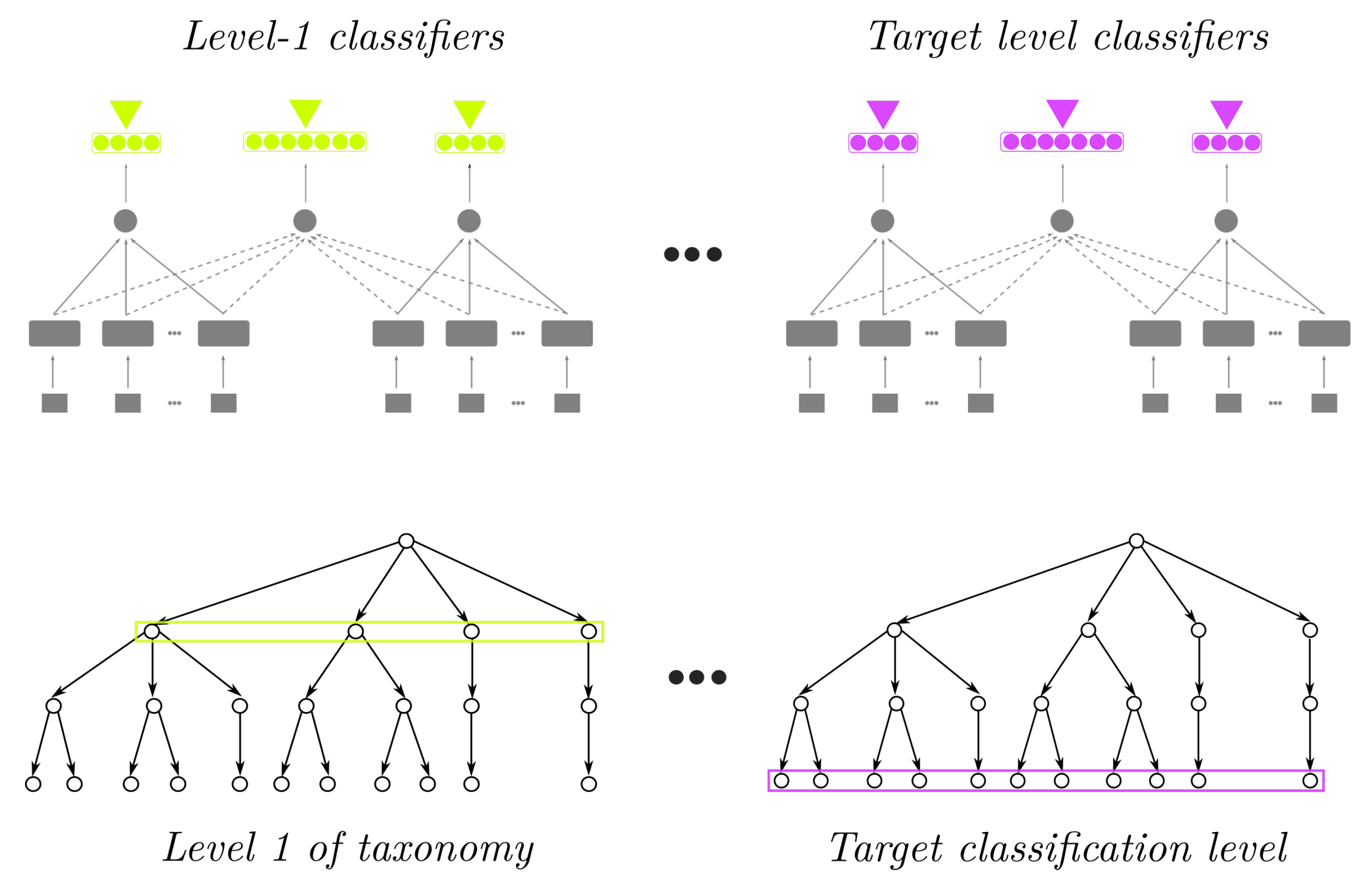
3.4. Hierarchical Pretraining Strategy

With the aim to leverage specific domain knowledge about the LULC classes, the HOb2sRNN parameters were learned exploiting the taxonomic organization associated to the classes. The training of the model is repeated for each level of the taxonomy, from the more general to the most specific (the target classification level). Specifically, we start training the model from the highest level of the hierarchy and then, continue training at the next level by reusing the previously learned weights for the whole architecture, excepting those that are associated to the classifiers, since level specific (see Figure 8). New weights were learned for the classifiers at each level of the taxonomy. The process is performed until we reach the target classification level. In summary, the hierarchical pretraining strategy allows for the model to focus first on high level classification problems (i.e., crops vs non crops) and, step by step, to smoothly adapt its behaviour to deal with classification problems of increasing complexity. In addition, this process allows the model to tackle the classification at the target level integrating a kind of prior knowledge on the task (based on high level classes) instead of addressing it completely from scratch.

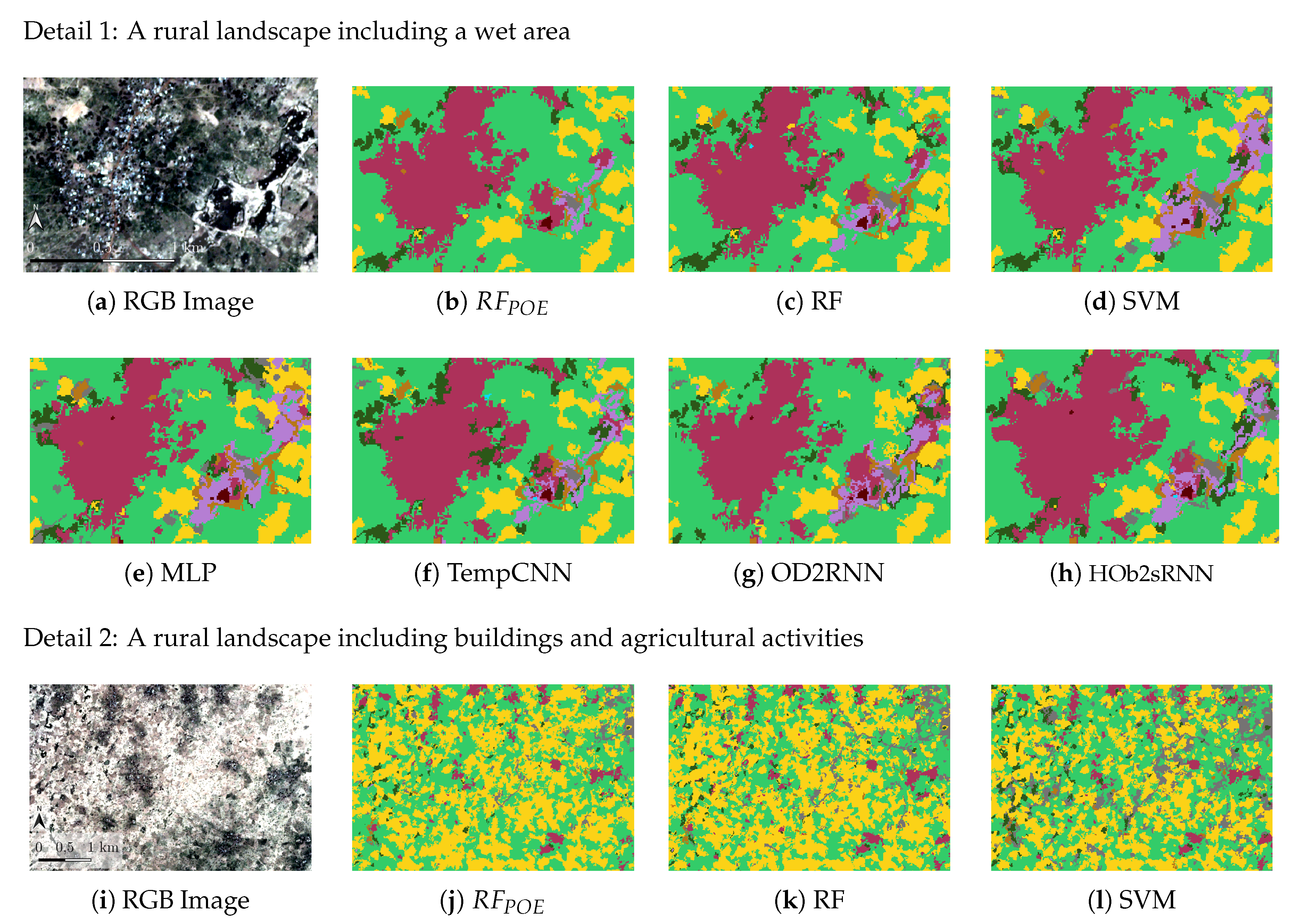
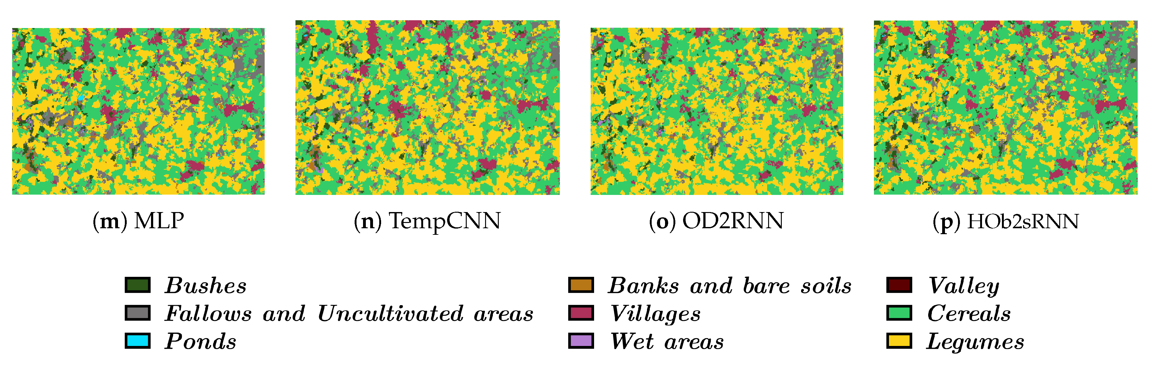
4. Experiments

In this section, we present and examine the experimental results obtained on the study sites introduced in Section 2. We carried out several experimental analysis to provide a deep assessment of the HOb2sRNN behaviour:

• an in-depth evaluation of the quantitative performances of HOb2sRNN model with respect to several other competitors;
• a sensitivity analysis of the $\alpha$ hyperparameter to weight the auxiliary classifier contributions and an ablation study of input sources and main components of the architecture in order to characterize the interplay among them;
• a qualitative analysis of land cover maps produced by HOb2sRNN and its competitors; and,
• an inspection of the attention parameters learnt by the HOb2sRNN model with the aim to investigate to what extent such side information contributes to the model interpretability.

4.1. Experimental Settings

To assess the quality of HOb2sRNN, we chose several approaches as competitors: a version of the Random Forest classifier that works on the early fusion of the radar/optical sources: the radar and optical information are concatenated together and the model is fed with this information [17] (RF); a version of the Random Forest classifier that works on the late fusion of the source information, as described in [42]: a RF model is trained for each of the input sources and, then, the combination is achieved via the product of per-source RF model outputs (RF${}_{\mathbf{POE}}$); a Support Vector Machine (SVM), a Multi Layer Perceptron (MLP) as the one employed as main classifier of the HOb2sRNN architecture, the Temporal Convolutional Neural Network (TempCNN) proposed by [43] that performs convolutions on the temporal dimension of the time series information and the OD2RNN model proposed in [15]. Like the RF, the SVM and MLP models were run on the concatenation of the multi-temporal and multi-source data. For the TempCNN model, we set up an architecture with 2 branches, one per source, sharing the same convolutional structure as described in [43]. The outputs of the two branches were successively concatenated and fed into the classifier module. The OD2RNN model was employed with the same structure and parametrization considered in [15]. Trainable parameters of neural network approaches i.e., MLP, TempCNN, OD2RNN, and HOb2sRNN models are reported in

Table 3. Trainable parameters of neural network approaches i.e., MLP, TempCNN, OD2RNN, and HOb2sRNN on both study sites.

Trainable Parameters	Reunion	Senegal
MLP	349,195	332,809
TempCNN	465,739	268,617
OD2RNN	2,173,761	2,160,667
HOb2sRNN	4,391,810	4,382,576

.

The values of the datasets were normalized per band, when considering the time series, in the interval $[0,1]$. The datasets were split into training, validation and test set with a proportion of 50%, 20% and 30% of samples (labeled segments), respectively. We imposed that segments belonging to the same ground truth polygon before the spatial intersection (see Section 2.3) were exclusively assigned to one of the data partition (training, validation or test) with the aim to avoid possible spatial bias in the evaluation procedure. The models were optimized via training/validation procedure [28] (settings are reported in

Table 4. Hyperparameter settings of the competing methods. RF and SVM method hyperparamaters were optimized by varying associated values while MLP, TempCNN, OD2RNN and HOb2sRNN model hyperparameters were empirically fixed.

Method	Hyperparameter	Value or Range
RF	Number of trees	{100, 200, 300, 400, 500}
	Maximum depth	{20, 40, 60, 80, 100}
	Maximum features	{’sqrt’, ’log2’, None}
SVM	Kernel	{’linear’, ’poly’, ’rbf’, ’sigmoid’}
	Gamma	{0.25, 0.5, 1,2}
	Penalty	{0.1, 1, 10}
MLP	Hidden units	512
	Hidden layers	2
	Dropout rate	0.4
HOb2sRNN	FCGRU units	512 for each hidden state
	$F{C}_1$ units	64
	$F{C}_2$ units	128
	Main classifier units	512 for each layer
	Dropout rate	0.4
All neural network models	Batch size	32
	Optimizer	Adam [45]
	Learning rate	1 × 10−4
	Number of epochs	2000 (per level for HOb2sRNN)

). Their assessment was done using test set and considering following metrics: Accuracy (global precision), F1 score (harmonic mean of precision and recall), and Cohen’s Kappa (level of agreement between two raters relative to chance). Because the model performances may vary depending on the split of the data due to simpler or more complex samples involved in the different partitions, all metrics were averaged over ten random splits of the datasets following the strategy mentioned above. Experiments were carried out on a workstation with an Intel Xeon CPU, 256 GB of RAM and four TITAN X GPU. In such environment, the HOb2sRNN model takes approximately 16 h (resp. 4.5 h) to complete training on Reunion island (resp. Senegalese site) while testing needs around one minute on both study sites. The neural net models were implemented using the Python Tensorflow library, while other implementations were obtained from the Python Scikit-learn library [44]. The implementation of the HOb2sRNN model is available at https://github.com/eudesyawog/HOb2sRNN.

4.2. Comparative Analysis

In this evaluation, we compare the results that were obtained by the different competing methods, considering their overall and per-class behaviours.

4.2.1. General Behaviour

Table 5. F1 score, Kappa, and Accuracy considering the different methods on each study site (results averaged over ten random splits). We have highlighted the best scores in bold.

Reunion	F1 Score	Kappa	Accuracy
RF${}_{POE}$	74.26 ± 0.75	0.713 ± 0.009	74.72 ± 0.78
RF	75.62 ± 1.00	0.726 ± 0.011	75.75 ± 0.98
SVM	75.34 ± 0.88	0.722 ± 0.010	75.39 ± 0.89
MLP	77.96 ± 0.70	0.752 ± 0.008	78.03 ± 0.66
TempCNN	77.76 ± 1.06	0.749 ± 0.012	77.79 ± 1.05
OD2RNN	74.39 ± 1.14	0.712 ± 0.012	74.50 ± 1.09
HOb2sRNN	79.66 ± 0.85	0.772 ± 0.009	79.78 ± 0.82
Senegal	F1 Score	Kappa	Accuracy
RF${}_{POE}$	85.31 ± 0.50	0.816 ± 0.006	85.45 ± 0.48
RF	86.31 ± 0.91	0.828 ± 0.012	86.35 ± 0.90
SVM	89.95 ± 0.85	0.875 ± 0.011	89.96 ± 0.85
MLP	90.05 ± 0.56	0.876 ± 0.007	90.07 ± 0.57
TempCNN	88.81 ± 0.58	0.861 ± 0.007	88.83 ± 0.58
OD2RNN	88.35 ± 0.72	0.855 ± 0.009	88.34 ± 0.72
HOb2sRNN	90.78 ± 1.03	0.885 ± 0.013	90.78 ± 1.03

reports the average performances obtained on the two study sites. We can note that the proposed method outperformed its competitors on both study sites, although the performance gap is more pronounced on the Reunion island dataset than on the Senegalese site. This behaviour may be due to the fact that the Reunion island benchmark has more ground truth samples (about eight times) than the Senegalese dataset. In fact, deep learning models are known to be effective when trained on huge volumes of data. Concerning the other competing methods, RF and SVM achieve similar scores on the Reunion island, while SVM surpasses RF on the Senegalese site. On this latter benchmark, the SVM algorithm demonstrates to be well suited for dataset characterized by a limited set of labeled samples. We also note that, on both study sites, the $R{F}_{POE}$ competitor was less effective than the RF variant which is fed with the concatenated sources. As regards the MLP and TempCNN competitors, both achieved lower scores than HOb2sRNN on the Reunion island, while the performance of the MLP is comparable to that of HOb2sRNN on the Senegalese site. Moreover, the OD2RNN model performances on both study sites indicate the added value of extensions provided by the HOb2sRNN model. It should be noted that the relatively better performance obtained on the Senegalese site compared to the Reunion island (90.78 vs. 79.66) may come from the topography of the two sites. In fact, Reunion island is characterized by a rugged topography while the Senegalese site is essentially flat. Relief effects, like shadow or orientation, can induce biases in the discrimination of land cover classes impacting much more the Reunion island [14].

4.2.2. Per-Class Analysis

Figure 9 and Figure 10 show the per-class F1 scores obtained by the different methods on the Reunion island and the Senegalese site, respectively. Concerning the Reunion site, we can observe that HOb2sRNN achieves the best performances on the majority of land cover classes excepted some classes where other competing methods i.e., RF or MLP obtained slightly better scores that are still comparable to the ones achieved by our framework. It is worth noting how the proposed method outperforms its competitors particularly on agricultural/vegetation classes such as Sugarcane, Pasture and fodder, Market gardening or Orchards. This particular efficiency on such classes suggests that the HOb2sRNN architecture is well suited to deal with the temporal dependencies characterizing these land cover classes. As regards the Senegalese site, HOb2sRNN per-class scores are moderate. It achieved the best scores on 4 land cover classes over 9 namely Fallows, Ponds, Cereals and Legumes while other competing methods outperformed its results especially on the Valley class. Nonetheless, it should be remarked that also in this case, HOb2sRNN obtained the best results on land cover classes that exhibit a time-varying behaviour. It is common to observe natural vegetation activity on fallows areas; ponds appear during the rainy season while cereals and legumes follow crop growth cycle. These findings are inline with the previous observations made on the Reunion island and confirm the fact that the proposed method is capable to leverage temporal dependencies to made its decisions. To go further with the per-class analysis, we also investigated the confusions matrices of each method on the two study sites. Concerning the Reunion island (Figure 11), all of the methods exhibit similar behaviours. This is particularly evident between Greenhouse crops and Urbanized areas classes even if confusions between land cover classes are reduced from $R{F}_{POE}$ (Figure 11a) to HOb2sRNN (Figure 11b) as can be observed. Overall, the per-class analysis is coherent with the findings we got from the previous analysis. Apropos of the Senegalese site (Figure 12), confusions vary sensibly regarding the different methods. $R{F}_{POE}$ (Figure 12a) and RF (Figure 12b) exhibits more confusions on Bushes and Fallows classes that are highly misclassified with Cereals and a little bit less with Legumes, while Ponds are often confused with Wet areas. The other competitors tend to reduce these confusions, as underlined by their confusion matrix.

4.3. Sensitivity and Ablation Analysis

In this part of the evaluation, we conduct a sensitivity analysis regarding the influence of the weights of the auxiliary classifiers and, then, we perform several ablation studies to better characterize the behaviour of our framework. For the latter point, we considered the role of multi-source information (radar vs optical SITS), the role of the different architecture components disentangling their contributions and the interplay between spectral bands and radiometric indices (NDVI) regarding the optical signal.

4.3.1. Sensitivity Analysis on the Weights of Per-Source Auxiliary Classifiers

Here, we analyse how the $\alpha$ weights that are associated to the contribution of the auxiliary classifiers influence the classification performances of our framework. To this end, we vary $\alpha$ in the range [0.1, 0.7] with a step of 0.1 and we consider the F1 score measure. Figure 13 reports the results of such analysis. Regarding the Senegal study site, the F1 score varies from 89.35 when $\alpha$ is equal to 0.1 to 90.78 when $\alpha$ is equal to 0.5. Concerning the Reunion study site, the F1 score varies from 79.02 when $\alpha$ is equal to 0.4 to 79.87 when the weight is equal to 0.6.

Generally, we can note that all of the obtained F1 score are competitive w.r.t. the behaviour exhibited by the other methods (see Table 5) and, the performances of HOb2sRNN are quite stable when considering the different values on which $\alpha$ ranges.

4.3.2. Ablation on the Multi-Source Data

In this stage of experiments, we considered only one source time series (radar or optical) to perform the land cover classification. An unique branch was employed for the TempCNN, OD2RNN and HOb2sRNN models. Regarding the results that are reported in

Table 6. F1 score, Kappa, and Accuracy of the different methods considering the per-source ablation analysis on the Reunion island (results averaged over ten random splits). We have highlighted the best scores in bold.

Sentinel-1	F1 Score	Kappa	Accuracy
RF	36.77 ± 0.93	0.291 ± 0.011	37.85 ± 0.95
SVM	6.56 ± 0.36	0.018 ± 0.009	16.85 ± 0.53
MLP	34.93 ± 1.42	0.271 ± 0.016	36.01 ± 1.39
TempCNN	32.28 ± 1.19	0.239 ± 0.013	33.17 ± 1.17
OD2RNN	31.83 ± 0.98	0.234 ± 0.012	32.71 ± 1.01
HOb2sRNN	31.80 ± 1.10	0.231 ± 0.011	32.39 ± 1.04
Sentinel-2	F1 Score	Kappa	Accuracy
RF	76.24 ± 0.59	0.732 ± 0.007	76.32 ± 0.63
SVM	75.55 ± 0.80	0.724 ± 0.009	75.60 ± 0.80
MLP	77.95 ± 0.69	0.751 ± 0.008	77.98 ± 0.73
TempCNN	78.25 ± 0.88	0.755 ± 0.010	78.27 ± 0.90
OD2RNN	74.55 ± 0.81	0.714 ± 0.008	74.66 ± 0.72
HOb2sRNN	78.69 ± 0.95	0.761 ± 0.010	78.79 ± 0.91
RF${}_{POE}$	74.26 ± 0.75	0.713 ± 0.009	74.72 ± 0.78
RF	75.62 ± 1.00	0.726 ± 0.011	75.75 ± 0.98
SVM	75.34 ± 0.88	0.722 ± 0.010	75.39 ± 0.89
MLP	77.96 ± 0.70	0.752 ± 0.008	78.03 ± 0.66
TempCNN	77.76 ± 1.06	0.749 ± 0.012	77.79 ± 1.05
OD2RNN	74.39 ± 1.14	0.712 ± 0.012	74.50 ± 1.09
HOb2sRNN	79.66 ± 0.85	0.772 ±0.009	79.78 ± 0.82

and

Table 7. F1 score, Kappa, and Accuracy of the different methods when considering the per-source ablation analysis on the Senegalese site (results averaged over ten random splits). We have highlighted the best scores in bold.

Sentinel-1	F1 Score	Kappa	Accuracy
RF	75.71 ± 1.03	0.703 ± 0.013	76.56 ± 1.00
SVM	71.27 ± 0.82	0.653 ± 0.010	72.82 ± 0.78
MLP	78.96 ± 1.28	0.738 ± 0.015	79.05 ± 1.23
TempCNN	77.79 ± 0.79	0.725 ± 0.010	78.01 ± 0.80
OD2RNN	75.07 ± 1.59	0.692 ± 0.019	75.34 ± 1.50
HOb2sRNN	77.42 ± 1.33	0.721 ± 0.016	77.63 ± 1.27
Sentinel-2	F1 Score	Kappa	Accuracy
RF	84.51 ± 1.17	0.806 ± 0.015	84.60 ± 1.17
SVM	88.64 ± 0.47	0.858 ± 0.006	88.63 ± 0.45
MLP	88.38 ± 0.61	0.855 ± 0.008	88.40 ± 0.62
TempCNN	87.42 ± 1.02	0.843 ± 0.013	87.42 ± 1.04
OD2RNN	86.03 ± 0.75	0.826 ± 0.010	86.01 ± 0.75
HOb2sRNN	87.56 ± 1.33	0.845 ± 0.017	87.55 ± 1.33
Both Sources	F1 Score	Kappa	Accuracy
RF${}_{POE}$	85.31 ± 0.50	0.816 ± 0.006	85.45 ± 0.48
RF	86.31 ± 0.91	0.828 ± 0.012	86.35 ± 0.90
SVM	89.95 ± 0.85	0.875 ± 0.011	89.96 ± 0.85
MLP	90.05 ± 0.56	0.876 ± 0.007	90.07 ± 0.57
TempCNN	88.81 ± 0.58	0.861 ± 0.007	88.83 ± 0.58
OD2RNN	88.35 ± 0.72	0.855 ± 0.009	88.34 ± 0.72
HOb2sRNN	90.78 ± 1.03	0.885 ± 0.013	90.78 ± 1.03

, the radar time series has a specific behaviour for each of the considered study site. If radar signal is quite discriminating on the Senegalese site, this is not really the same for the Reunion island, considering how poorly the competing methods trained on the radar SITS performed, especially the SVM algorithm. As mentioned earlier (Section 4.2.1), the Reunion island is characterized by a rugged relief compared to the Senegalese site which is almost flat. Because radar signal is much more sensitive to high ground relief than optical, the performances of the competing methods are negatively impacted when trained with radar data only on the Reunion. Thus, the majority of the models i.e., (RF, SVM, MLP, TempCNN, and OD2RNN) performed slightly worst or equally when combining both sources due to the noise that seems to come from the radar signal. However, HOb2sRNN was able to better leverage the complementarity between radar and optical data to improve with both sources. This behaviour is also noticeable on the Senegalese site where HOb2sRNN achieved better performances than its competitors even though all the competitors improved with both sources. For the rest, regardless of the study site, there is no trend on which competing the method better deals with radar or optical time series. Nonetheless, we have observed on both sites that the SVM algorithm seems not well suited to exploit radar information.

4.3.3. Ablation on the Main Components of the Architecture

In this part, we investigate the interplay among the different components of HOb2sRNN and we disentangle their benefits in the architecture. We considered both time series (radar and optical), but excluded one of the following components at a time: the three attention mechanisms involved in the architecture (naming $\mathbf{NoAtt}$), the hierarchical pretraining process (naming $\mathbf{NoHierPre}$) and the enrichment step involved the FCGRU cell which is equivalent to using a GRU cell (naming $\mathbf{NoEnrich}$). We also investigated the use of traditional $SoftMax$ attention mechanism instead of the modified one in the HOb2sRNN architecture. More in detail, this variant also involves the feature enrichment component in the FCGRU cell and the hierarchical pretraining process. We named it $\mathbf{SoftMaxAtt}$. The results are reported in

Table 8. F1 score, Kappa, and Accuracy considering different ablations of HOb2sRNN on the study sites (results averaged over ten random splits). We have highlighted the best scores in bold.

Reunion	F1 Score	Kappa	Accuracy
$noAtt$	77.66 ± 0.99	0.749 ± 0.011	77.74 ± 0.99
$SoftMaxAtt$	77.32 ± 1.22	0.746 ± 0.013	77.47 ± 1.18
$noHierPre$	78.35 ± 0.70	0.756 ± 0.007	78.43 ± 0.66
$noEnrich$	79.09 ± 0.57	0.764 ± 0.006	79.10 ± 0.50
HOb2sRNN	79.66 ± 0.85	0.772 ± 0.009	79.78 ± 0.82
Senegal	F1 Score	Kappa	Accuracy
$noAtt$	89.86 ± 0.62	0.874 ± 0.008	89.89 ± 0.63
$SoftMaxAtt$	89.91 ± 0.54	0.874 ± 0.007	89.92 ± 0.52
$noHierPre$	89.25 ± 0.88	0.866 ± 0.011	89.24 ± 0.87
$noEnrich$	89.12 ± 0.64	0.864 ± 0.008	89.11 ± 0.64
HOb2sRNN	90.78 ± 1.03	0.885 ± 0.013	90.78 ± 1.03

. Concerning the use of attention mechanisms or not ($NoAtt$, $SoftMaxAtt$ and HOb2sRNN), we can observe how these components contribute to the final classification performances on both study sites, more on the Reunion island (about 2 points of improvement) than the Senegalese site (approximately one point). We can also note that the $SoftMaxAtt$ variant performs similarly to the $NoAtt$ variant and lower than the HOb2sRNN architecture confirming our hypothesis that relaxing the constraint that the attention weights may sum to 1 in the attention process could be more suitable for remote sensing context. As regards the use of the hierarchical pretraining process ($noHierPre$ vs HOb2sRNN), we can note the added value of such step on both study sites obtaining more than 1 point of improvement. These results seem to underline that involving domain specific knowledge in the pretraining process of neural networks can improve the final classification performances. Finally, the enrichment step carried out in the FCGRU cell ($noEnrich$ vs. HOb2sRNN) also demonstrates its usefulness in both study sites, however it seems to be more effective on the Senegalese site.

4.3.4. Ablation on Optical Information

We evaluate here whether the NDVI index as additional optical descriptor has an impact on the final land cover classification obtained using the HOb2sRNN architecture. Indeed, considering NDVI index as additional feature in land cover classification task was obvious when training conventional machine learning algorithms, since such techniques cannot extract specialized features for a specific task at hand [46]. Nowadays, the new paradigm related to deep (representational) learning [46] is emerging and demonstrating to be more and more effective in the field of remote sensing [47]. Neural networks have the ability to extract features optimised for a specific task (when enough data are available) avoiding the necessity to extract hand-crafted features. Thus, employing spectral indices, like NDVI, as additional features to deal with land cover classification could not be necessary when using neural networks. Therefore, we evaluate on the two study sites our model performances while excluding the NDVI index from the input (optical) time series. We named such variant $\mathbf{noNDVI}$. The results are reported in

Table 9. F1 score, Kappa, and Accuracy when considering the exclusion of Normalized Difference Vegetation Index (NDVI) index on the study sites (results averaged over ten random splits). We have highlighted the best scores in bold.

Reunion	F1 Score	Kappa	Accuracy
$noNDVI$	79.83 ± 0.70	0.774 ± 0.008	79.95 ± 0.68
HOb2sRNN	79.66 ± 0.85	0.772 ± 0.009	79.78 ± 0.82
Senegal	F1 Score	Kappa	Accuracy
$noNDVI$	90.46 ± 0.82	0.881 ± 0.010	90.46 ± 0.82
HOb2sRNN	90.78 ± 1.03	0.885 ± 0.013	90.78 ± 1.03

.

We can note on both study sites that there is no significant difference in the model performance when NDVI is excluded. $noNDVI$ performs slightly better than HOb2sRNN on the Reunion island and inversely on the Senegalese site. These small variations come from model properties such as kernel weight initialization or parameter optimization that can induce such kind of performance fluctuations. To conclude, this experiment underlines that our model, considering the two study sites involved in the experimental evaluation, is able to overcome the use of such common hand-crafted features achieving the same performances in the land cover classification task. Such a result makes a step further on the comprehension of which hand-crafted features are convenient (or not) to be extracted during the preprocessing step as well as save time, computation, and storage resources during the analysis pipeline.

4.4. Qualitative Analysis of Land Cover Maps

With the purpose to investigate some differences in the land cover maps produced by the competing methods, we highlight in Figure 14 and Figure 15 some representative map details of the Reunion island and the Senegalese site, respectively. For each study site, we remind that land cover maps were produced by labeling each of the segments (14,465 on the Reunion island or 116,937 on the Senegalese site) obtained after the VHSR image segmentation (SPOT6/7 or PlanetScope). For each example, we supplied the corresponding VHSR image displayed in RGB colour as reference. Concerning Reunion island, we focused in the first example (Figure 14b–h), on the Saint-Pierre mixed coastal urban and agricultural area. In this example, we can note the confusions highlighted in the per-class analysis between urbanized areas and greenhouse crops. Visually, RF models ($R{F}_{POE}$ particularly) better classifies urbanized areas. The second example (Figure 14j–p) depicts a mixed agricultural area with natural vegetation neighboring. We can note here that HOb2sRNN detects a realistic amount of orchards with respect to other methods, according to field experts. In addition, we can also observe on the right of this extract that RF wrongly classified as sugar cane plantations some wooded areas, moor, and savannah objects. Moreover, at the bottom left of the OD2RNN map, we can highlight the misclassification that arises between Rocks and Water classes. Regarding the Senegalese site, the first example (Figure 15b–h) depicts a wet area near the Diohine village located in the east. While other competitors tend to provide the correct representation of the wet area, RF methods wrongly detect villages. As pointed out in previous map details concerning Sugarcane and Orchards on the Reunion island study site, RF predictions is sometimes biased towards most represented classes in the training data i.e., Sugarcane, Orchards in the case of Reunion island and Villages here. In fact, RF is known to be sensible to class imbalance [48]. The second example (Figure 15j–p) focused on a rural landscape, including built-up (villages) and agricultural activities. Here, RF models map more legumes than the other methods while the rest of the approaches detect fallows and cereals instead. To sum up, these visual inspections of land cover maps are consistent with the previously obtained quantitative results.

4.5. Attention Parameters Analysis

In this last part of our experimental results, we explore the side information provided by the attention mechanism introduced in Section 3.2 in order to get meaningful insights about how HOb2sRNN handles the multi-source time series for the land cover classification task. Attention weights have been successfully employed in the field of NLP [36,38,49] to explain which parts of the input signal contribute to the final decision of RNN models. With the aim to set up an analogous analysis in the remote sensing time series classification context, we considered attention weights on the Senegalese site with a particular interest on crops (cereals and legumes) motivated by the agronomic knowledge we obtained from discussions with field experts.

Figure 16 depicts the distribution of the attention weights on cereals and legumes land covers. For the sake of simplicity, we only focused on the attention mechanism employed to support the fused classifier. At first glance, we can observe that the model weights quite similarly the radar and optical time stamps on both classes. We can also notice that some time stamps towards the end of each time series are highly weighted. It is interesting to note that correlation exists between these high attention values and the crops growth. In the Senegalese groundnut basin, vegetation reaches its peak activity, in fact, during the August month (middle of the time series) also characterized by heavy rain amount, all inducing more differentiation among land cover classes. However, on the two last optical time stamps (25/10/2018 and 30/10/2018), attention weights were differently attributed when considering the two crop types. Cereals get more important weights for these two timestamps than legumes. This behaviour seems to be associated to the agricultural practices adopted in the area at the end of the season. While cereals (mainly millet) are harvested cutting only the ears, legumes (mainly groundnut) are torn off. Thus, on these latter time stamps, cereal plots are covered by senescent plants while legume plots turn into bare soils. These practices are visible in the SITS and illustrated in Figure 17. To wrap up this analysis, we have observed that correlations exist between the attention weights learnt by HOb2sRNN and agricultural practices that characterized the considered study areas. As underlined by our findings, the exploration of the attention parameters can support the understanding of the decision made by our model and provides useful insights about the information that is contained in the SITS under the lens of agricultural field practices.

5. Discussion

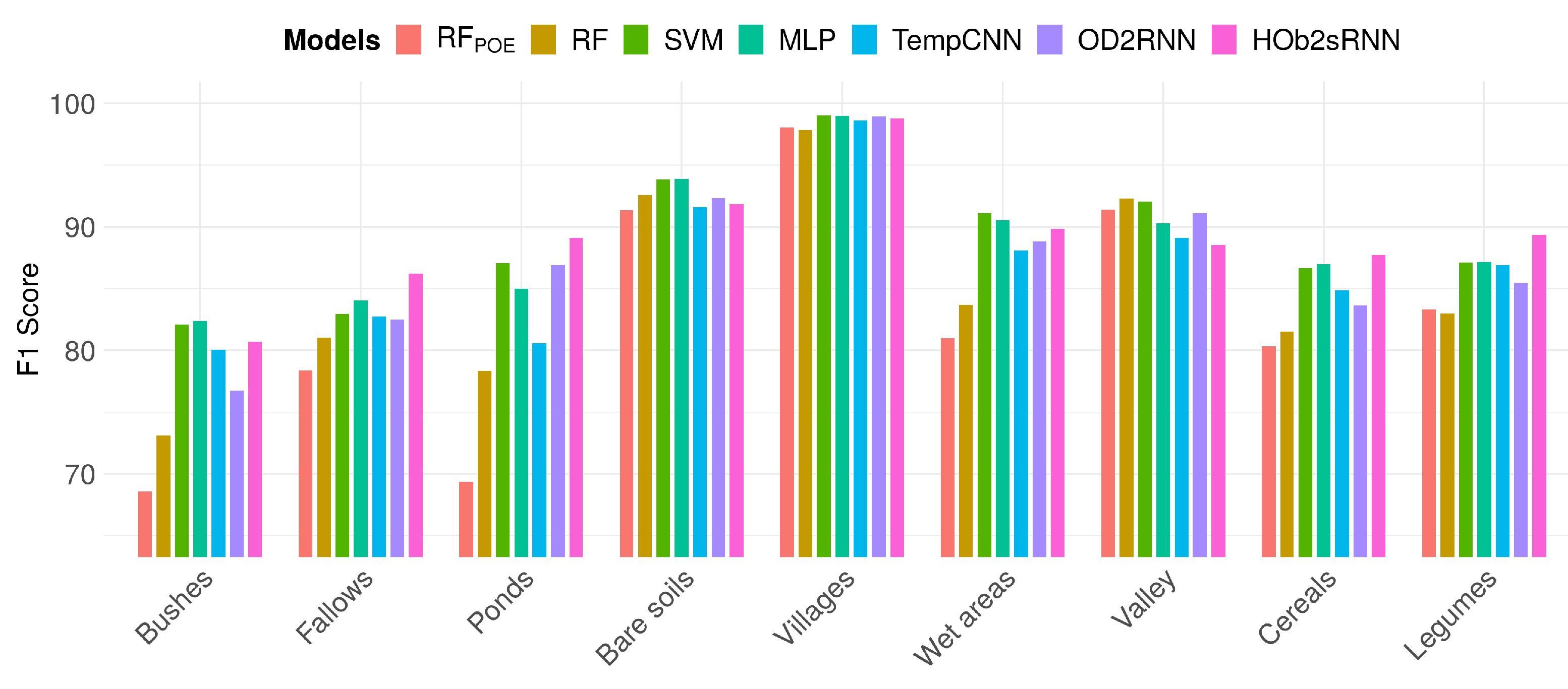
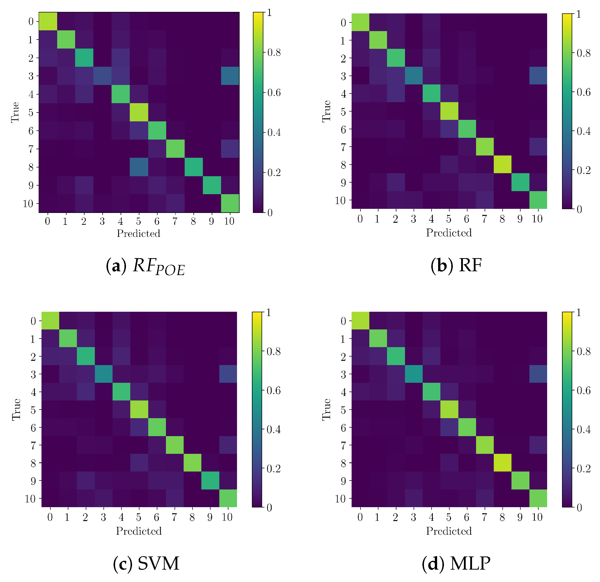
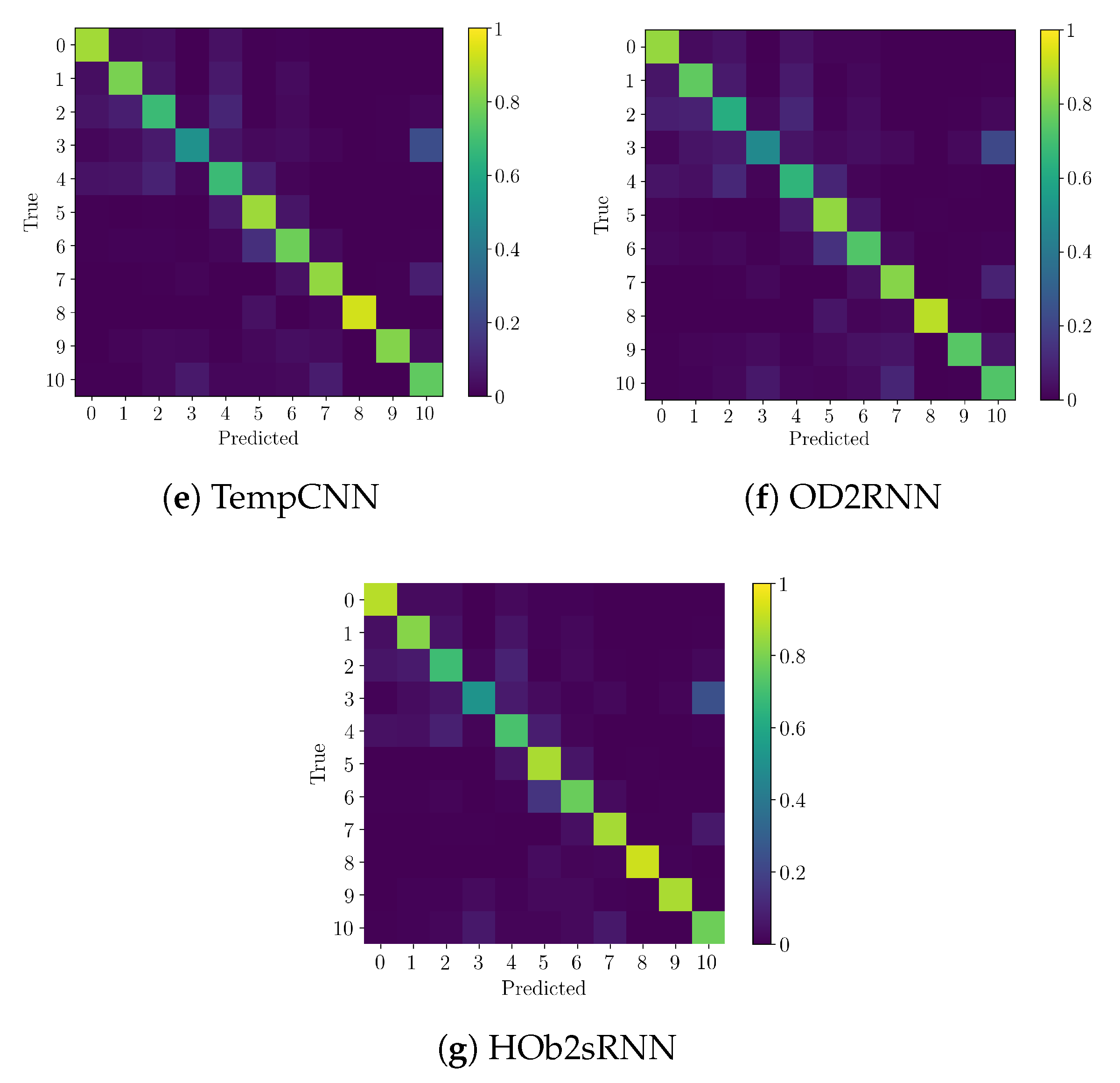
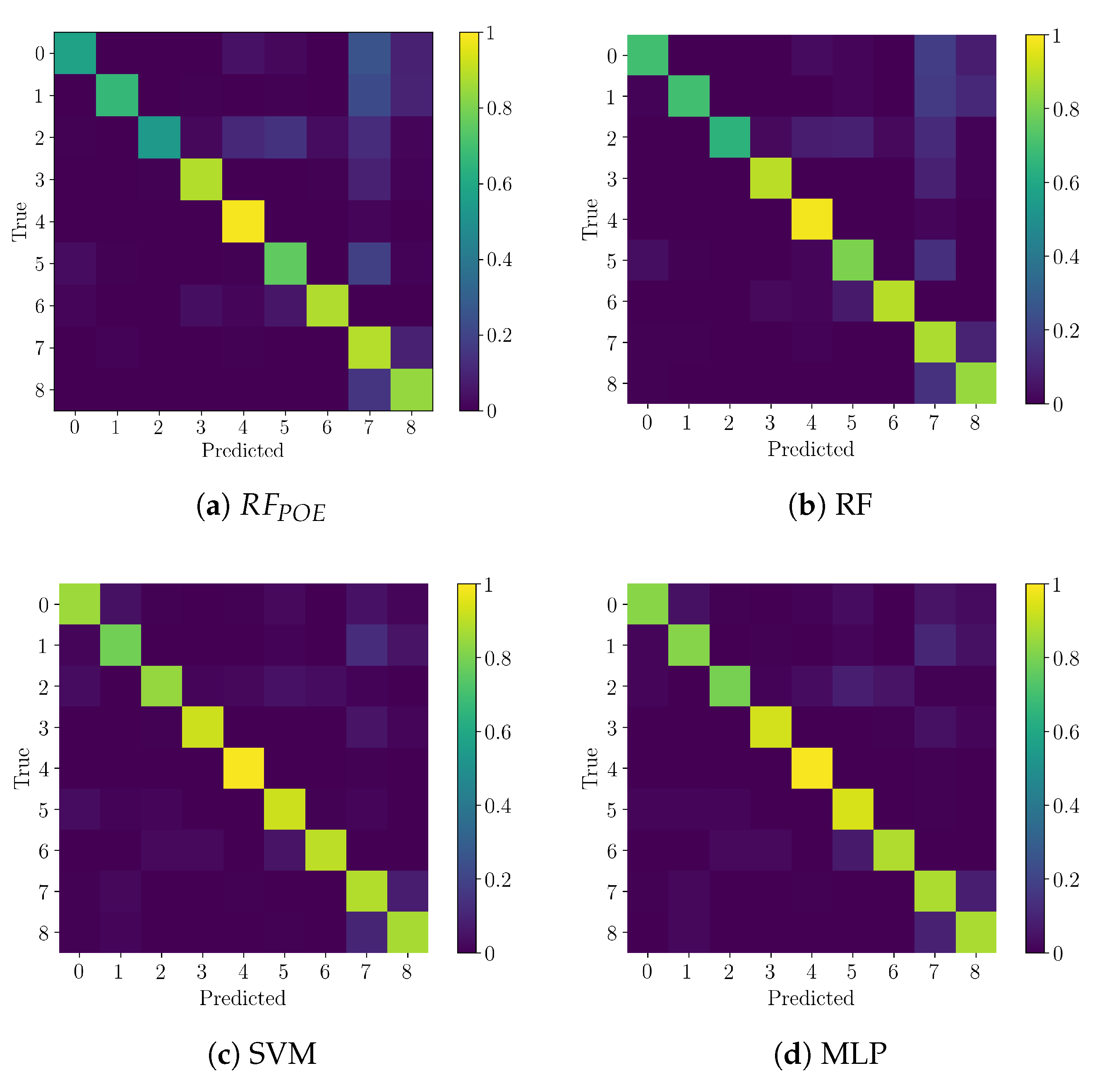
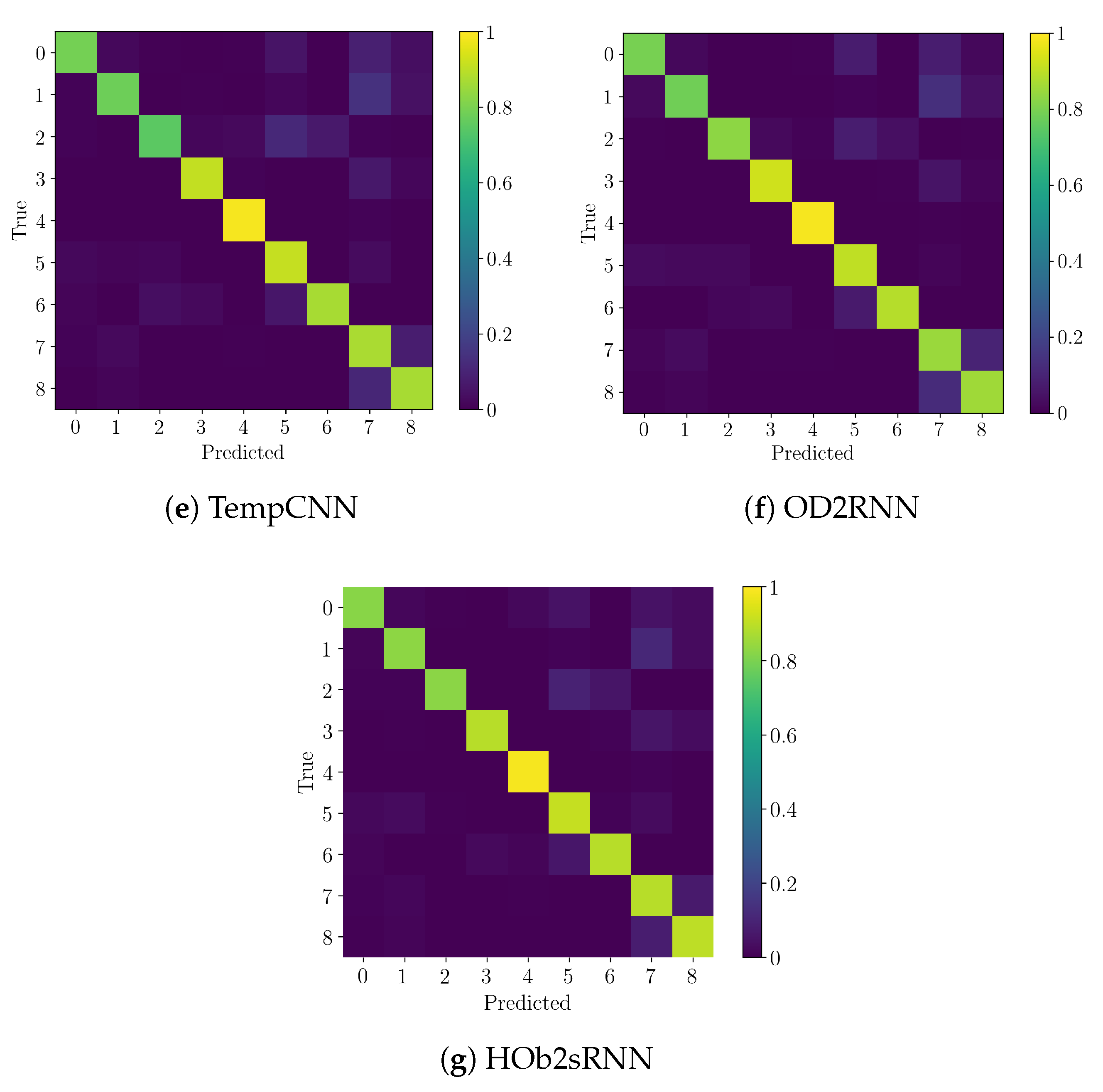
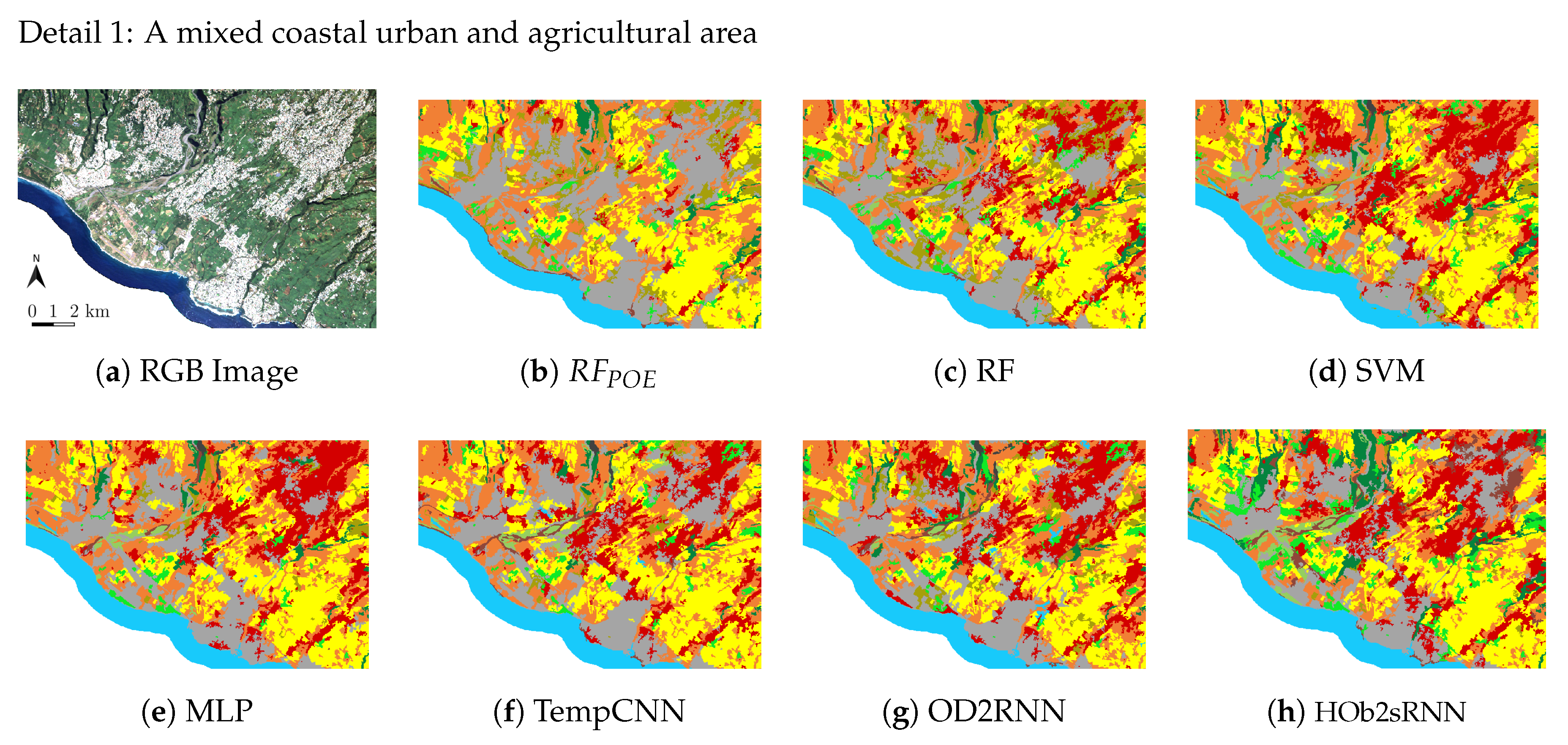
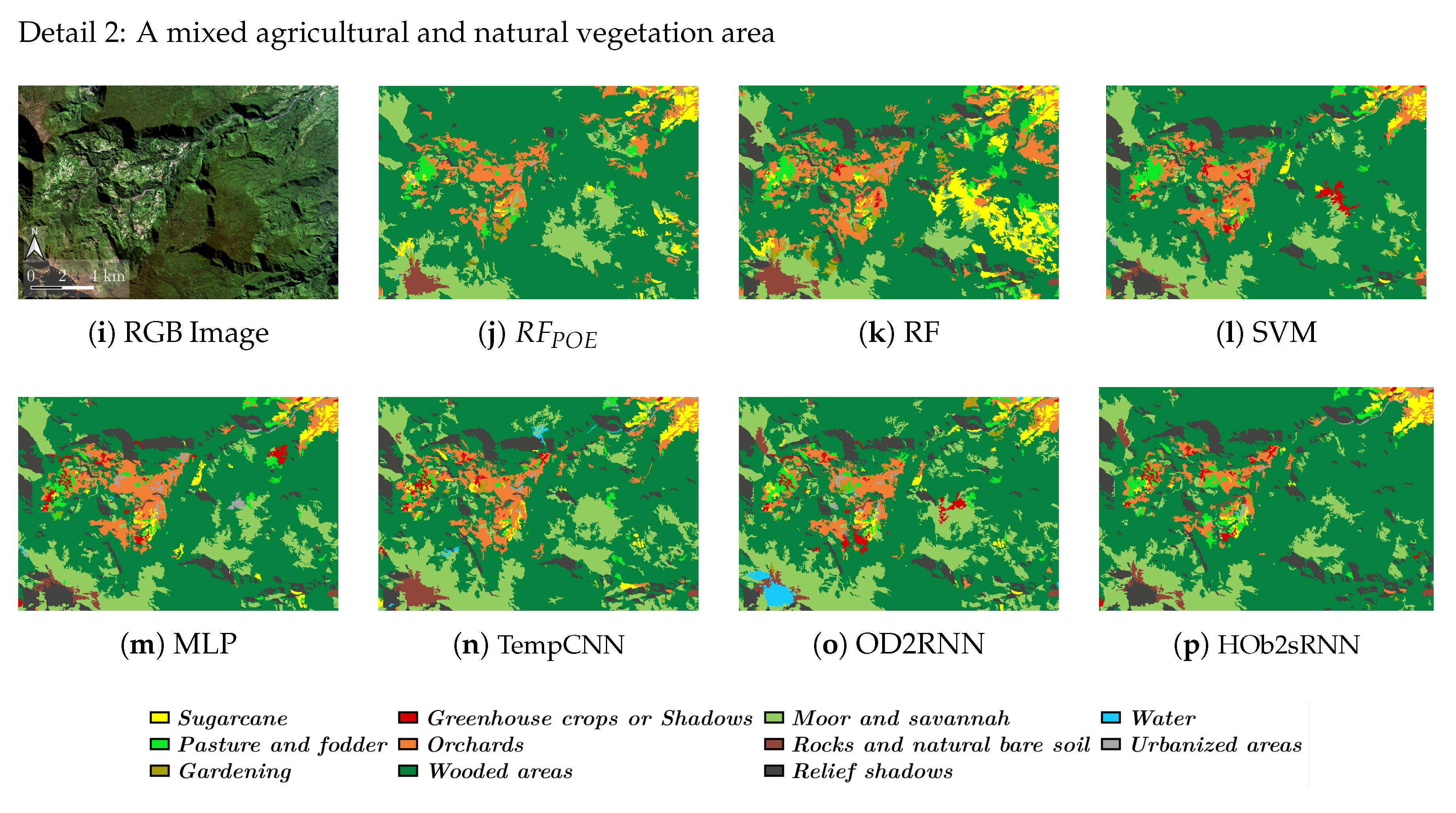
To summarize, the proposed deep learning framework exhibits convincing performances in land cover mapping considering situations characterized by a realistic amount of available training samples. The comparison with other machine learning approaches underlines three points: (i) our approach clearly outperforms the RF classifier that is a common strategy employed to deal with SITS classification; (ii) other standard machine learning methods, i.e., SVM and MLP, exhibit competitive behaviours with respect to our method on a study site that involves a small amount of labeled samples; and, (iii) our proposal surpasses, on both study sites, the adaptation of the recent TempCNN competitor for the multi-source scenario. Such result points out again that, beyond modelling the temporal correlation exhibited by SITS data via RNN or CNN approaches, in a multi-source context other features be worthy to be considered: the hierarchical class relationships as well as the way in which radar/optical information may be combined.

The ablation study indicates that HOb2sRNN is capable to exploit the complementarity between the radar and optical information, always improving its performances with respect to using only one of the two sources. Our framework integrates background knowledge via hierarchical pretraining leveraging taxonomic relationships between land cover classes. The experiments highlight that such knowledge seems valuable for the model and it systematically ameliorates its behaviour. On the other hand, some other type of considered knowledge, i.e., the NDVI index, seems less effective due to the fact that, probably, the model is capable to overcome it. Such observation was also highlighted by [43]. These points clearly pave the way to further investigation about which and how knowledge can be injected to guide/regularize the learning process of such techniques. In addition, the analysis conducted on the $\alpha$ hyperparameter demonstrates that the integration of the auxiliary classifiers, in the training procedure, brings added value still considering small weighting values.

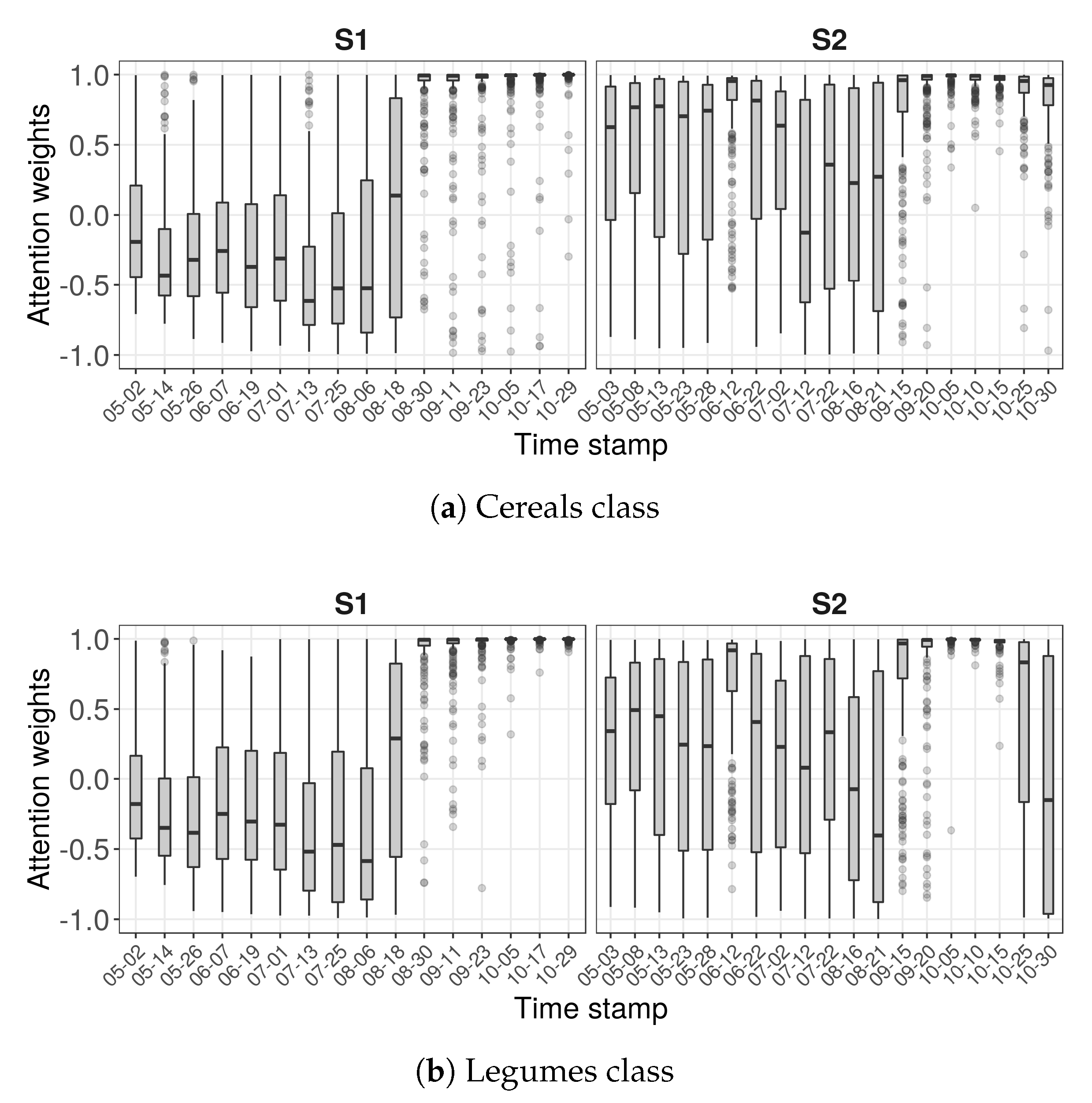
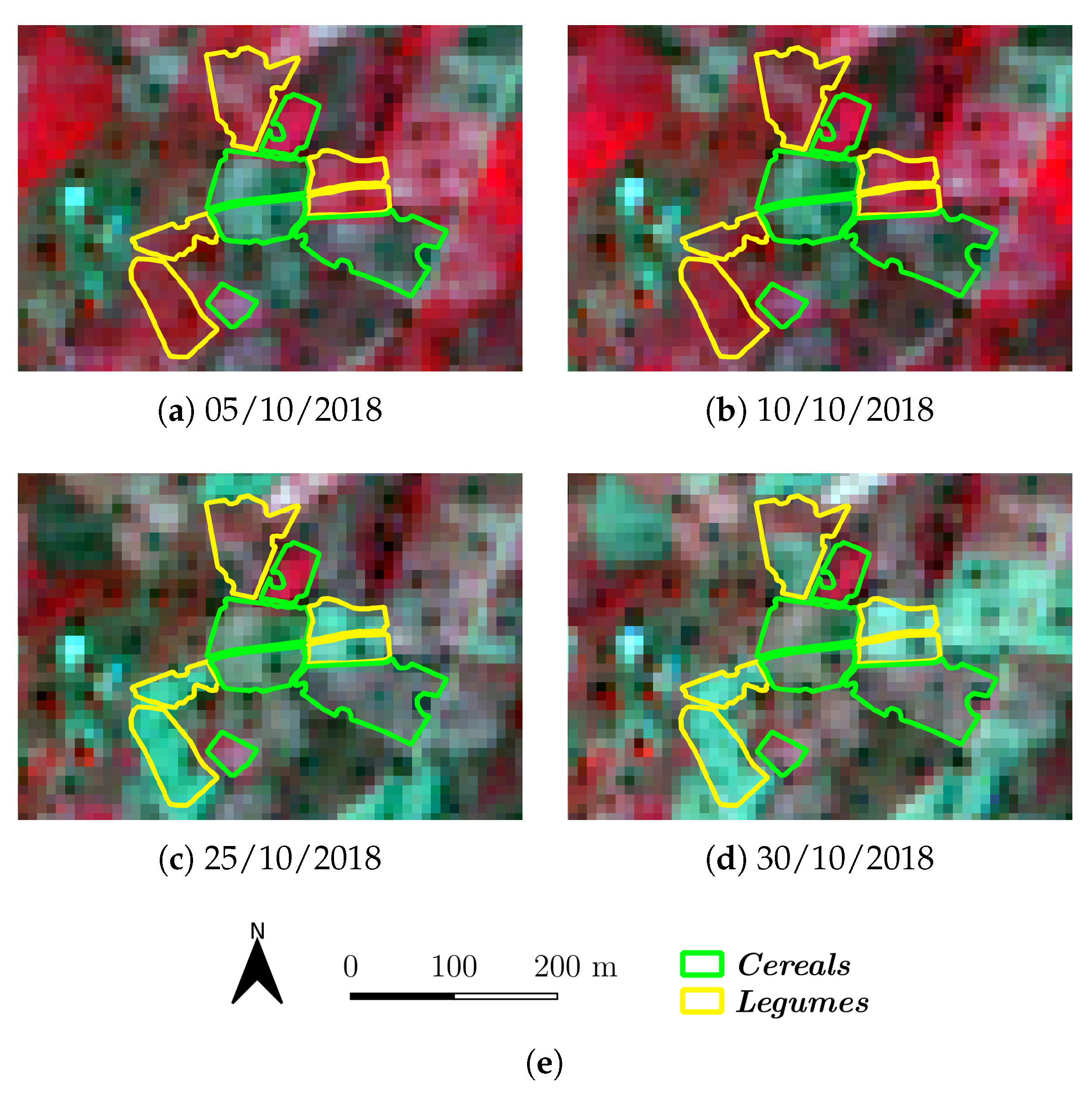
When considering the model interpretability, we have also provided some qualitative studies about the side information that can be extracted from our framework. The qualitative results we obtain are in line with the agronomic knowledge we obtained from the considered study area. Make the black box grey is an hot topic today in the machine learning community [50] and we can state, with a certain margin of confidence, that solutions or answers associated to this question will be available in a near future.

We recall that our framework works under an OBIA setting. This means that its performances are tightly related to the quality of the underlying segmentation process that is sensitive to several elements [51], for example: the employed segmentation algorithm, since different algorithms show different pros and cons; the determination of the scale parameter for the particular segmentation algorithm, since useful information can be available at different scales and the co-registration among different sources when working with multi-source data. If on one side, all of these elements carrying in opportunities to properly model the underlying information available in the considered remote sensing data for the analysis at hand, on the other side they can constitute possible sources of errors that are propagated until the land cover mapping result. We underline that it is out of the scope of this work to investigate how such elements impact the subsequent analysis since they deserve a complete and extensive study also in light of the recent adoption of deep learning techniques in the remote sensing domain. Here, we have focused our effort on the multi-source land cover mapping task assuming that the object layer, derived by the segmentation, is an input of our framework. For this reason, we believe that progress in the OBIA field, improving the extraction of the object layer from remote sensing data, can only ameliorate downstream analysis, like the one proposed in this work.

Finally, we remind that operational/realistic constraints might be considered when dealing with remote sensing analysis. Constraints can be related to available resources, i.e., timely production of land cover maps or limited access to training samples. We are aware that, in operational/realistic scenario characterized by the almost real-time production of land cover maps (i.e., disaster management [52]), more computationally efficient solutions needs to be preferred (i.e., MLP or SVM) to deep learning approaches. On the other hand, in our work, we deal with (agricultural-oriented) land cover mapping where, land cover maps need to be provided with a relative low time frequency (once or twice per year). Due to this fact, here, the operational constraints are mainly intended regarding the limited amount of available labeled samples. In such data paucity setting, our approach clearly outperforms the Random Forest classifier, which is the de facto strategy involved in the operational classification of SITS data [53]. In addition, the experimental evaluation pointed out that, less explored machine learning techniques in the context of SITS analysis, i.e., SVM and MLP, deserve much attention, since they constitute valuable strategies to which compare future proposals.

6. Conclusions

In this work, we propose dealing with land cover mapping at object level, from multi-temporal and multi-source (radar and optical) data. Our approach is based on an enriched RNN cell and involved a modified attention mechanism devised to better suit the SITS data context. We also introduce a hierarchical pretraining approach for the architecture which integrates specific knowledge from land cover classes to support the land cover mapping task. Extensive quantitative and qualitative evaluations on two study sites demonstrate the effectiveness of our solution as compared to competitive approaches in the field of land cover mapping with SITS data. As future work, we plan to extend the current framework in order to also leverage spatial dependencies in multi-source SITS, which are often neglected, especially in the OBIA setting. In addition, the great popularity of Transformer models [54] in the field of Natural Language Processing for handling sequential data makes them a potential way of fusing multi-temporal and multi-source remote sensing data in subsequent research.

References

1. Berger, M.; Moreno, J.; Johannessen, J.A.; Levelt, P.F.; Hanssen, R.F. ESA’s sentinel missions in support of Earth system science. Remote Sens. Environ. 2012, 120, 84–90. [Google Scholar] [CrossRef]
2. Kolecka, N.; Ginzler, C.; Pazur, R.; Price, B.; Verburg, P.H. Regional Scale Mapping of Grassland Mowing Frequency with Sentinel-2 Time Series. Remote Sens. 2018, 10, 1221. [Google Scholar] [CrossRef] [Green Version]
3. Kussul, N.; Lavreniuk, M.; Skakun, S.; Shelestov, A. Deep Learning Classification of Land Cover and Crop Types Using Remote Sensing Data. IEEE Geosci. Remote Sens. Lett. 2017, 14, 778–782. [Google Scholar] [CrossRef]
4. Inglada, J.; Vincent, A.; Arias, M.; Tardy, B.; Morin, D.; Rodes, I. Operational High Resolution Land Cover Map Production at the Country Scale Using Satellite Image Time Series. Remote Sens. 2017, 9, 95. [Google Scholar] [CrossRef] [Green Version]
5. Guttler, F.; Ienco, D.; Nin, J.; Teisseire, M.; Poncelet, P. A graph-based approach to detect spatiotemporal dynamics in satellite image time series. ISPRS J. Photogramm. Remote Sens. 2017, 130, 92–107. [Google Scholar] [CrossRef] [Green Version]
6. Khiali, L.; Ienco, D.; Teisseire, M. Object-oriented satellite image time series analysis using a graph-based representation. Ecol. Inform. 2018, 43, 52–64. [Google Scholar] [CrossRef] [Green Version]
7. Steinhausen, M.J.; Wagner, P.D.; Narasimhan, B.; Waske, B. Combining Sentinel-1 and Sentinel-2 data for improved land use and land cover mapping of monsoon regions. Int. J. Appl. Earth Obs. Geoinf. 2018, 73, 595–604. [Google Scholar] [CrossRef]
8. Minh, D.H.T.; Ienco, D.; Gaetano, R.; Lalande, N.; Ndikumana, E.; Osman, F.; Maurel, P. Deep Recurrent Neural Networks for Winter Vegetation Quality Mapping via Multitemporal SAR Sentinel-1. IEEE Geosci. Remote Sens. Lett. 2018, 15, 464–468. [Google Scholar] [CrossRef]
9. Gbodjo, Y.J.E.; Ienco, D.; Leroux, L. Toward Spatio-Spectral Analysis of Sentinel-2 Time Series Data for Land Cover Mapping. IEEE Geosci. Remote Sens. Lett. 2019, 17, 307–311. [Google Scholar] [CrossRef]
10. Interdonato, R.; Ienco, D.; Gaetano, R.; Ose, K. DuPLO: A DUal view Point deep Learning architecture for time series classificatiOn. ISPRS J. Photogramm. Remote Sens. 2019, 149, 91–104. [Google Scholar] [CrossRef] [Green Version]
11. Mousavi, S.M.; Roostaei, S.; Rostamzadeh, H. Estimation of flood land use/land cover mapping by regional modelling of flood hazard at sub-basin level case study: Marand basin. Geomat. Nat. Hazards Risk 2019, 10, 1155–1175. [Google Scholar] [CrossRef] [Green Version]
12. Fritz, S.; See, L.; Bayas, J.C.L.; Waldner, F.; Jacques, D.; Becker-Reshef, I.; Whitcraft, A.; Baruth, B.; Bonifacio, R.; Crutchfield, J.; et al. A comparison of global agricultural monitoring systems and current gaps. Agric. Syst. 2019, 168, 258–272. [Google Scholar] [CrossRef]
13. Gao, F.; Masek, J.G.; Schwaller, M.R.; Hall, F.G. On the blending of the Landsat and MODIS surface reflectance: Predicting daily Landsat surface reflectance. IEEE Trans. Geosci. Remote Sens. 2006, 44, 2207–2218. [Google Scholar]
14. Ienco, D.; Interdonato, R.; Gaetano, R.; Minh, D.H.T. Combining Sentinel-1 and Sentinel-2 Satellite Image Time Series for land cover mapping via a multi-source deep learning architecture. ISPRS J. Photogramm. Remote Sens. 2019, 158, 11–22. [Google Scholar] [CrossRef]
15. Ienco, D.; Gaetano, R.; Interdonato, R.; Ose, K.; Minh, D.H.T. Combining Sentinel-1 and Sentinel-2 Time Series via RNN for Object-Based Land Cover Classification. In Proceedings of the 2019 IEEE International Geoscience and Remote Sensing Symposium (IGARSS 2019), Yokohama, Japan, 28 July–2 August 2019; pp. 4881–4884. [Google Scholar]
16. Iannelli, G.C.; Gamba, P. Jointly Exploiting Sentinel-1 and Sentinel-2 for Urban Mapping. In Proceedings of the 2018 IEEE International Geoscience and Remote Sensing Symposium (IGARSS 2018), Valencia, Spain, 22–27 July 2018; pp. 8209–8212. [Google Scholar]
17. Erinjery, J.; Singh, M.; Kent, R. Mapping and assessment of vegetation types in the tropical rainforests of the Western Ghats using multispectral Sentinel-2 and SAR Sentinel-1 satellite imagery. Remote Sens. Environ. 2018, 216, 345–354. [Google Scholar] [CrossRef]
18. Tricht, K.V.; Gobin, A.; Gilliams, S.; Piccard, I. Synergistic Use of Radar Sentinel-1 and Optical Sentinel-2 Imagery for Crop Mapping: A Case Study for Belgium. Remote Sens. 2018, 10, 1642. [Google Scholar] [CrossRef] [Green Version]
19. Denize, J.; Hubert-Moy, L.; Betbeder, J.; Corgne, S.; Baudry, J.; Pottier, E. Evaluation of using sentinel-1 and-2 time-series to identify winter land use in agricultural landscapes. Remote Sens. 2019, 11, 37. [Google Scholar] [CrossRef] [Green Version]
20. Fernández-Beltran, R.; Haut, J.M.; Paoletti, M.E.; Plaza, J.; Plaza, A.; Pla, F. Multimodal Probabilistic Latent Semantic Analysis for Sentinel-1 and Sentinel-2 Image Fusion. IEEE Geosci. Remote Sens. Lett. 2018, 15, 1347–1351. [Google Scholar] [CrossRef]
21. Di Gregorio, A. Land Cover Classification System: Classification Concepts and User Manual: LCCS; Food & Agriculture Organization: Rome, Italy, 2005; Volume 2. [Google Scholar]
22. Sulla-Menashe, D.; Friedl, M.A.; Krankina, O.N.; Baccini, A.; Woodcock, C.E.; Sibley, A.; Sun, G.; Kharuk, V.; Elsakov, V. Hierarchical mapping of Northern Eurasian land cover using MODIS data. Remote Sens. Environ. 2011, 115, 392–403. [Google Scholar] [CrossRef]
23. Wu, M.F.; Sun, Z.C.; Yang, B.; Yu, S.S. A Hierarchical Object-oriented Urban Land Cover Classification Using WorldView-2 Imagery and Airborne LiDAR data. IOP Conf. Ser. Earth Environ. Sci. 2016, 46, 012016. [Google Scholar] [CrossRef]
24. Sulla-Menashe, D.; Gray, J.M.; Abercrombie, S.P.; Friedl, M.A. Hierarchical mapping of annual global land cover 2001 to present: The MODIS Collection 6 Land Cover product. Remote Sens. Environ. 2019, 222, 183–194. [Google Scholar] [CrossRef]
25. Blaschke, T. Object based image analysis for remote sensing. ISPRS J. Photogramm. Remote Sens. 2010, 65, 2–16. [Google Scholar] [CrossRef] [Green Version]
26. Lillesand, T.; Kiefer, R.W.; Chipman, J. Remote Sensing and Image Interpretation; John Wiley & Sons: Hoboken, NJ, USA, 2015. [Google Scholar]
27. Zhu, X.; Tuia, D.; Mou, L.; Zhang, G.X.L.; Xu, F.; Fraundorfer, F. Deep Learning in Remote Sensing: A Comprehensive Review and List of Resources. IEEE Geosci. Remote Sens. Mag. 2017, 5, 8–36. [Google Scholar] [CrossRef] [Green Version]
28. Ienco, D.; Gaetano, R.; Dupaquier, C.; Maurel, P. Land Cover Classification via Multitemporal Spatial Data by Deep Recurrent Neural Networks. IEEE Geosci. Remote Sens. Lett. 2017, 14, 1685–1689. [Google Scholar] [CrossRef] [Green Version]
29. Mou, L.; Ghamisi, P.; Zhu, X.X. Unsupervised Spectral-Spatial Feature Learning via Deep Residual Conv-Deconv Network for Hyperspectral Image Classification. IEEE Trans. Geosci. Remote Sens. 2018, 56, 391–406. [Google Scholar] [CrossRef] [Green Version]
30. Zhong, L.; Hu, L.; Zhou, H. Deep learning based multi-temporal crop classification. Remote Sens. Environ. 2019, 221, 430–443. [Google Scholar] [CrossRef]
31. Rußwurm, M.; Körner, M. Multi-Temporal Land Cover Classification with Sequential Recurrent Encoders. ISPRS Int. J. Geo-Inf. 2018, 7, 129. [Google Scholar] [CrossRef] [Green Version]
32. Rouse, J.W.; Hass, R.H.; Schell, J.; Deering, D. Monitoring vegetation systems in the great plains with ERTS. In Proceedings of the Third Earth Resources Technology Satellite (ERTS) symposium, Washington, DC, USA, 10–14 December 1973; Volume 1, pp. 309–317. [Google Scholar]
33. Dupuy, S.; Gaetano, R.; Mézo, L.L. Mapping land cover on Reunion Island in 2017 using satellite imagery and geospatial ground data. Data Brief 2020, 28, 104934. [Google Scholar] [CrossRef]
34. Lassalle, P.; Inglada, J.; Michel, J.; Grizonnet, M.; Malik, J. A Scalable Tile-Based Framework for Region-Merging Segmentation. IEEE Trans. Geosci. Remote Sens. 2015, 53, 5473–5485. [Google Scholar] [CrossRef]
35. Cho, K.; Van Merrienboer, B.; Gülçehre, Ç.; Bahdanau, D.; Bougares, F.; Schwenk, H.; Bengio, Y. Learning Phrase Representations using RNN Encoder-Decoder for Statistical Machine Translation. arXiv 2014, arXiv:1406.1078. [Google Scholar]
36. Bahdanau, D.; Cho, K.; Bengio, Y. Neural Machine Translation by Jointly Learning to Align and Translate. arXiv 2014, arXiv:1409.0473. [Google Scholar]
37. Luong, M.; Pham, H.; Manning, C.D. Effective Approaches to Attention-based Neural Machine Translation. In Proceedings of the 2015 Conference on Empirical Methods in Natural Language Processing (EMNLP 2015), Lisbon, Portugal, 17–21 September 2015; pp. 1412–1421. [Google Scholar]
38. Britz, D.; Guan, M.Y.; Luong, M. Efficient Attention using a Fixed-Size Memory Representation. arXiv 2017, arXiv:1707.00110. [Google Scholar]
39. Karamanolakis, G.; Hsu, D.; Gravano, L. Weakly Supervised Attention Networks for Fine-Grained Opinion Mining and Public Health. arXiv 2019, arXiv:1910.00054. [Google Scholar]
40. Hou, S.; Liu, X.; Wang, Z. DualNet: Learn Complementary Features for Image Recognition. In Proceedings of the IEEE International Conference on Computer Vision, Venice, Italy, 22–29 October 2017; pp. 502–510. [Google Scholar]
41. Benedetti, P.; Ienco, D.; Gaetano, R.; Ose, K.; Pensa, R.G.; Dupuy, S. M3 Fusion: A Deep Learning Architecture for Multiscale Multimodal Multitemporal Satellite Data Fusion. IEEE J. Sel. Top. Appl. Earth Obs. Remote Sens. 2018, 11, 4939–4949. [Google Scholar] [CrossRef] [Green Version]
42. Valero, S.; Arnaud, L.; Planells, M.; Ceschia, E.; Dedieu, G. Sentinel’s Classifier Fusion System for Seasonal Crop Mapping. In Proceedings of the 2019 IEEE International Geoscience and Remote Sensing Symposium (IGARSS 2019), Yokohama, Japan, 28 July–2 August 2019; pp. 6243–6246. [Google Scholar]
43. Pelletier, C.; Webb, G.; Petitjean, F. Temporal Convolutional Neural Network for the Classification of Satellite Image Time Series. Remote Sens. 2019, 11, 523. [Google Scholar] [CrossRef] [Green Version]
44. Pedregosa, F.; Varoquaux, G.; Gramfort, A.; Michel, V.; Thirion, B.; Grisel, O.; Blondel, M.; Prettenhofer, P.; Weiss, R.; Dubourg, V.; et al. Scikit-learn: Machine Learning in Python. J. Mach. Learn. Res. 2011, 12, 2825–2830. [Google Scholar]
45. Kingma, D.P.; Ba, J. Adam: A Method for Stochastic Optimization. arXiv 2014, arXiv:1412.6980. [Google Scholar]
46. Lecun, Y.; Bengio, Y.; Hinton, G. Deep learning. Nature 2015, 521, 436–444. [Google Scholar] [CrossRef]
47. Ma, L.; Liu, Y.; Zhang, X.; Ye, Y.; Yin, G.; Johnson, B.A. Deep learning in remote sensing applications: A meta-analysis and review. ISPRS J. Photogramm. Remote Sens. 2019, 152, 166–177. [Google Scholar] [CrossRef]
48. Maxwell, A.E.; Warner, T.A.; Fang, F. Implementation of machine-learning classification in remote sensing: An applied review. Int. J. Remote Sens. 2018, 39, 2784–2817. [Google Scholar] [CrossRef] [Green Version]
49. Choi, H.; Cho, K.; Bengio, Y. Fine-grained attention mechanism for neural machine translation. Neurocomputing 2018, 284, 171–176. [Google Scholar] [CrossRef] [Green Version]
50. Ribeiro, M.T.; Singh, S.; Guestrin, C. “Why Should I Trust You?”: Explaining the Predictions of Any Classifier. In Proceedings of the 22nd ACM SIGKDD International Conference on Knowledge Discovery and Data Mining, San Francisco, CA, USA, 13–17 August 2016; pp. 1135–1144. [Google Scholar]
51. Chen, G.; Weng, Q.; Hay, G.J.; He, Y. Geographic object-based image analysis (GEOBIA): Emerging trends and future opportunities. GISci. Remote Sens. 2018, 55, 159–182. [Google Scholar] [CrossRef]
52. Boccardo, P.; Tonolo, F.G. Remote sensing role in emergency mapping for disaster response. In Engineering Geology for Society and Territory—Volume 5; Springer: Berlin/Heidelberg, Germany, 2015; pp. 17–24. [Google Scholar]
53. Belgiu, M.; Drăguţ, L. Random forest in remote sensing: A review of applications and future directions. ISPRS J. Photogramm. Remote Sens. 2016, 114, 24–31. [Google Scholar] [CrossRef]
54. Vaswani, A.; Shazeer, N.; Parmar, N.; Uszkoreit, J.; Jones, L.; Gomez, A.N.; Kaiser, L.; Polosukhin, I. Attention is All you Need. In Proceedings of the Advances in Neural Information Processing Systems 30: Annual Conference on Neural Information Processing Systems 2017, Long Beach, CA, USA, 4–9 December 2017; pp. 5998–6008. [Google Scholar]
Figure 1. Overview of the acquisition dates of Sentinel-1 (S1) and Sentinel-2 (S2) images over the two study sites. S2 acquisitions were sparsed due to the ubiquitous cloudiness.
Remotesensing 12 02814 g001
Figure 2. Overview of the taxonomy derived from the Reunion island land cover classes.
Remotesensing 12 02814 g002
Figure 3. Overview of the taxonomy derived from the Senegalese site land cover classes.
Remotesensing 12 02814 g003
Figure 4. Some details about the segmentation performed on the Reunion island.
Remotesensing 12 02814 g004
Figure 5. Some details about the segmentation performed on the Senegalese site.
Remotesensing 12 02814 g005
Figure 6. Overview of the HOb2sRNN method. The architecture is composed of two branches, one for each source (radar and optical) SITS. Each branch processes the SITS by means of an enriched RNN cell we named FCGRU and an attention mechanism is employed on its outputs to extract the per source features. Furthermore, the same attention mechanism is employed on the concatenation of the per source outputs allowing to extract fused features. Finally, the per-source and fused feature sets are leveraged in order to provide the final classification.
Remotesensing 12 02814 g006
Figure 7. Visual representation of the GRU and FCGRU cells.
Remotesensing 12 02814 g007
Figure 8. Overview of the hierarchical pretraining strategy adopted for HOb2sRNN architecture.
Remotesensing 12 02814 g008
Figure 9. Per-Class F1 score for the Reunion island (average over ten random splits).
Remotesensing 12 02814 g009
Figure 10. Per-Class F1 score for the Senegalese site (average over ten random splits).
Remotesensing 12 02814 g010
Figure 11. Confusion matrices of the land cover classification produced by (a) R F P O E , (b) RF, (c) SVM, (d) MLP, (e) TempCNN, (f) OD2RNN and (g) HOb2sRNN on the Reunion island. See Table 1 for corresponding labels.
Remotesensing 12 02814 g011aRemotesensing 12 02814 g011b
Figure 12. Confusion matrices of the land cover classification produced by (a) R F P O E , (b) RF, (c) SVM, (d) MLP, (e) TempCNN, (f) OD2RNN and (g) HOb2sRNN on the Senegalese site. See Table 2 for corresponding labels.
Remotesensing 12 02814 g012aRemotesensing 12 02814 g012b
Figure 13. Sensitivity analysis of the α weights that are associated to the importance of the auxiliary classifiers in HOb2sRNN regarding the F1 score. Standard deviation is displayed as error bar.
Remotesensing 12 02814 g013
Figure 14. Qualitative investigation of land cover map details produced on the Reunion island study site over a mixed urban/agricultural area (top) and an agricultural/natural vegetation area (bottom).
Remotesensing 12 02814 g014aRemotesensing 12 02814 g014b
Figure 15. Qualitative investigation of land cover map details produced on the Senegalese study site over heterogeneous landscapes including buildings, agricultural, and wet areas.
Remotesensing 12 02814 g015aRemotesensing 12 02814 g015b
Figure 16. Box plots of the attention weights on cereals and legumes land covers considering the multi-source time series.
Remotesensing 12 02814 g016
Figure 17. Visualization of end of season agricultural practices in the Senegalese groundnut basin concerning cereals and legumes land covers. Background images come from the Sentinel-2 time series and are displayed in Green–Red–Infrared composite colours.
Remotesensing 12 02814 g017