Verification of Fractional Vegetation Coverage and NDVI of Desert Vegetation via UAVRS Technology

1
Shapotou Desert Research and Experiment Station, Northwest Institute of Eco-Environment and Resources, Chinese Academy of Sciences, Donggang West Road 320, Lanzhou 730000, China
2
Key Laboratory of Stress Physiology and Ecology in Cold and Arid Regions, Gansu Province, Lanzhou 730000, China
*
Author to whom correspondence should be addressed.
Remote Sens. 2020, 12(11), 1742; https://doi.org/10.3390/rs12111742
Submission received: 28 April 2020
/
Revised: 22 May 2020
/
Accepted: 22 May 2020
/
Published: 28 May 2020
(This article belongs to the Special Issue Silk-Road Disaster Monitoring and Risk Assessment Using Remote Sensing and GIS)
Abstract
:Desertification control and scientific evaluation of desert ecosystem sustainability are important issues for countries along the Silk Road Economic Belt. Fractional vegetation coverage (FVC) is used as a quantitative indicator to describe the vegetation coverage of desert ecosystems. Although satellite remote sensing technology has been widely used to retrieve FVC at the regional and global scale, the authenticity evaluation of the inversion results has been flawed. To gain insight into the composition, structure and changes of desert vegetation, it is important to assess the accuracy of FVC and explore the relationship between FVC and meteorological factors. Therefore, we adopted unmanned aerial vehicle remote sensing (UAVRS) technology to verify the inversion results and analyse the practicability of MODIS-NDVI (where NDVI = normalized difference vegetation index) products in desert areas. To provide a new method for the estimation of vegetation coverage in the natural state, the relationships between vegetation coverage and four meteorological factors, namely, land surface temperature, temperature, precipitation and evaporation were analysed. The results showed that using the original MODIS-NDVI data product with a spatial resolution of 250 m to invert vegetation coverage is practical in desert areas (coefficient of determination (R2) = 0.83, root mean square error (RMSE) = 0.052, normalized root mean square error (NRMSE) = 42.94%, mean absolute error (MAE) = 0.007) but underestimates vegetation coverage in the study area. MODIS-NDVI data products are different from the real NDVI in the study area. Correcting MODIS-NDVI data products can effectively improve the accuracy of the inversion. When extracting vegetation coverage in this area, the scale has little effect on the results. There is a significant correlation between precipitation, evaporation and FVC in the area, but the interaction of temperature and land surface temperature with precipitation and evaporation also has a considerable impact on FVC, and evaporation has a substantial impact on FVC values inverted from MODIS-NDVI data (FVCM), When exploring the relationship between vegetation coverage and meteorological elements, if vegetation coverage is retrieved from MODIS-NDVI data products or MODIS-NDVI data, when considering temperature and precipitation, the effect of evaporation should also be considered. In addition, meteorological factors can be used to predict FVC (R2 = 0.7364, RMSE = 0.0623), which provides a new method for estimating FVC in areas with less manual intervention.
1. Introduction
Vegetation, as an important part of terrestrial ecosystems, not only plays an important role in the processes of energy flow, ecohydrology, and the biogeochemical cycle but can also effectively prevent soil erosion, purify air, and maintain the stability of the ecological environment [1,2]. Accurate evaluation of vegetation coverage on the land surface helps us to understand the dynamics of land ecosystems [3]. Fractional vegetation coverage (FVC) is a quantitative parameter for describing the vegetation coverage on the land surface and the characteristics of ecosystems [1]. FVC is also an important input variable in weather forecast models, regional and global climate change models, and global climate change monitoring models that affect the accuracy of the prediction results [4,5]. Currently, the metabolic function of plants is being affected by global climate change, which may result in fluctuations in vegetation coverage [6]. Previous research showed that FVC in the middle and high latitudes of the Northern Hemisphere was increasing, and FVC in the arid regions of Northwest China was increasing significantly [7,8,9]. Therefore, accurate evaluation of FVC and exploration of the relationship between meteorological factors and FVC have great importance for improving the accuracy of model predictions and understanding regional ecological changes.
There are two main methods for calculating FVC, i.e., ground-based verification and remote sensing estimation [10,11]. Ground-based verification methods include visual estimation, sampling surveys, and photogrammetry [12]; however, these methods are usually affected by individual differences, weather, timing, and topographical factors. It is difficult to measure FVC in a large area, in general. FVC can only be estimated from survey information in limited areas such as specific plots or belt transects. Moreover, this method is more accurate in regions with homogeneous vegetation than heterogeneous vegetation [13]. Desert area is characterized by spatial heterogeneity, and the accuracy of FVC can be improved by increasing the sampling density or expanding the quadrate area. However, there are many difficulties in practical operation. Remote sensing inversion is a preferred and feasible way to estimate vegetation coverage. Compared with traditional ground-based verification, satellite remote sensing has the advantages of low requirements, rapid acquisition, and large area acquisition [1]. A number of methods for inverting FVC based on remotely sensed data exist, including empirical models [14], spectral mixing analysis [15], dimidiate pixel models [16], artificial neural networks [17], and regression trees [18]. Since the normalized difference vegetation index (NDVI) is sensitive to the spectral information of vegetation, it has been successfully used to monitor vegetation conditions and reflect growth status [19]. The two-endmember model divides a pixel into two types: vegetation and non-vegetation. The spectral information contained in one pixel of the image is also composed of non-vegetated and vegetation-covered areas [20]. Existing research has shown that there is a significant linear correlation between NDVI and FVC, and the dimidiate pixel model that combines the two-endmember model with NDVI can be used to invert FVC at the regional and global scales [16]. The accuracy of ground-based verification is high, but it is more difficult to measure on regional or global scales, especially in areas with high spatial heterogeneity leading to lower accuracy. Satellite remote sensing can solve the problem of vegetation inversion at the regional or global scale, however, due to the influence of soil type, humidity, and image resolution, the actual condition of ground vegetation is not truly retrievable, and the inversion accuracy is greatly dependent on the vegetation conditions. Hence, a method is needed to overcome the shortcomings of both satellite remote sensing and ground-based verification. Currently, a feasible solution is expected for solving such problems with the development of unmanned aerial vehicle remote sensing (UAVRS) technology.
Compared with satellite remote sensing platforms, UAVRS has the advantages of high spatiotemporal resolution, high mobility, good flexibility, robustness to weather conditions, and wide-ranging surveys, less affected by terrain and human resources compared with ground measurements [21]. UAVRS has been used in many fields, including ecological surveys [22], precision agriculture [23], and the estimation of FVC [24]. Chen et al. [25] noted that UAVRS could obtain high-resolution pictures to accurately extract vegetation coverage information, that was more accurate than ground measurements. Riihimakia et al. [26] demonstrated that satellite remote sensing data and UAVRS data can be combined to calculate FVC, and they studied a method that combines two types of data to invert vegetation coverage. Resolution of the images obtained by UAVRS is between that of the ground measurement data and satellite remote sensing images. When FVC is extracted at the regional or global scale, satellite remote sensing data are still the most important original data; however, UAVRS can be used to compensate for the errors caused by scale.
The objective of this study was to adopt UAVRS technology to verify the accuracy of FVC retrieved by satellite remote sensing products and further verify the practicality of MODIS-NDVI products in desert areas. The sampling plots were arranged in the temperate desert ecosystems of Alxa Plateau, Northwest China. FVC values from samples from photos taken by UAVs (FVCU).; meanwhile, the dimidiate pixel model was adopted to analyse the MODIS-NDVI data and to invert the FVC (FVCM). Then, the verification relationships between FVCU and FVCM were discussed. Moreover, the responses of the FVC of desert vegetation to hydrothermal gradients were analysed.We tested a new method for FVC estimation in desert regions and provided evidence for the scientific management of desert grasslands in the context of climate change.
2. Materials and Methods
2.1. Study Area
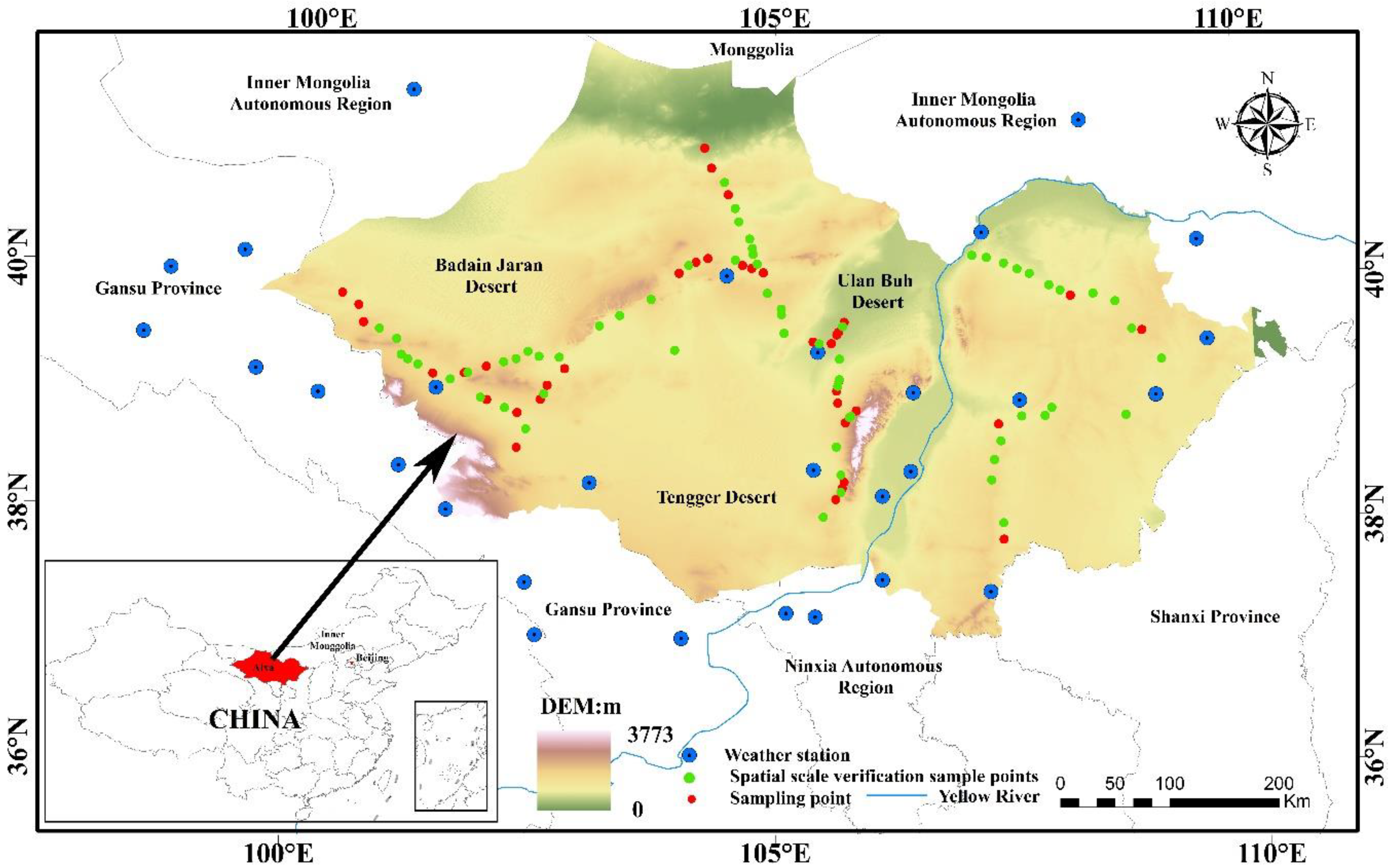
The Alxa Plateau lies in the eastern wing of the desert in central Asia (37°24′–42°47′N, 97°10′–106°53′E, Figure 1). It is adjacent to Mongolia in the north, Helan Mountain in the east, Mashan Mountain in the west, and the Tengger Desert in the south. The study area has a typical temperate continental climate, with a mean annual temperature of 6.8–8.8 °C, mean annual rainfall of 40–200 mm, and annual potential evapotranspiration of 1275–2204 mm. The terrain is high in the south and low in the north, and the altitude is between 900 and 1400 m. Deserts and desertified lands are widely distributed in the area, accounting for approximately 10% of the total area. Affected by extreme arid climate, the vegetation in this area grows intensively. In the southeast of the Helan Mountains, the vegetation type of the flood fan is desert steppe, and the other areas are mainly desert shrubs [27].
2.2. NDVI Data Acquisition
2.2.1. NDVI Data Acquisition by GreenSeeker Handheld Spectrometer
A GreenSeeker handheld spectrometer (Trimble, America) was used to collect actual NDVI values of the ground features. The GreenSeeker handheld spectrometer has been developed by Trimble’s agriculture division. The sensor has its own light source (active sensor), which allows measurements to be taken during the day or night. The sensor’s field of view is an oval whose size increases with the height of the sensor (approximately 10” wide at 24” above the ground, 20” wide at 48” above the ground) As a plat research and diagnostic tool, it can accurately measure and collect the vegetation NDVI and the ratio of red and near infrared spectra of vegetation and other materials. A GreenSeeker handheld spectrometer was used to collect NDVI values from 100 sampling plots in the study area. A 200-metre belt transect was set, and NDVI values were measured once every metre in each sampling plot. To maximize the field of view of the GreenSeeker handheld spectrometer, we tried to keep it as high as 1 metre during the acquisition process. An average of 200 NDVI values within the belt transect were considered as the real NDVI of each sampling plot. The data collection time was August 27 to September 8, 2017.
2.2.2. MODIS NDVI Data
The NDVI data collected by satellite remote sensing were derived from the MOD13Q1 data product in TERRA/MODIS-NDVI, with a spatial resolution of 250 m. The scanning and imaging times of the satellite images were almost in sync with the on-site survey, which was conducted on August 29, 2017. The downloaded MODIS-NDVI data were subjected to radiation calibration and atmospheric correction, eliminating data errors caused by atmospheric conditions, remote sensing platforms, working environments, solar altitude angles, and sensors. First, remotely sensed image data products covering the entire research area were downloaded from https://ladsweb.modaps.eosdis.nasa.gov. Then, the format and coordinates of the data were converted. The hierarchical data format (HDF) of the source data was converted to tiff format, and the sinusoidal map projection of the source data was converted to the WGS84 geographic coordinate system. Finally, the scope of the NDVI data file of the study area was defined based on the boundary map, and the NDVI values of each sampling plot were extracted using the corresponding latitude and longitude coordinates.
2.3. FVC Data Collection
2.3.1. Extracting FVC by UAVRS
The unmanned aerial vehicle (UAV ) used in the survey was a Phantom3 (SZ DJI Technology Co., Ltd., China), with a weight of 1216 g, horizontal flight speed of 16 m/s, and flight time of approximately 25 min. The effective pixel number of the camera was 12 million, the angle of view was 90 degrees, and the aperture was f/2.8. The software used to operate the UAV in this experiment was the FragMAP Locator APP for waypoint settings (Figure 2a) and the FragMAP Monitor APP for flight route settings (Figure 2b), and PixelClassifier software was used to process photos taken by the drone. These three software programs were developed by Professor Shu Hua Yi’s team, working on the application of drones in the ecological environment monitoring of fragile areas [28,29]. The flight mode was a grid flight mode, over a square quadrate of 200 × 200 m corresponding to a specific pixel of a remote sensing image. The quadrate was further divided into 9 equal squares with a total 16 vertices. The flight height of the drone was 20 m, the flight speed was 6 m/s, and the flight path is shown in the Figure 2c. The UAV took 16 photos at the vertex of each square at each sampling point, and obtained 10 photos of the same location at different heights in 67 samples. The collection time was from August 27 to September 8, 2017, and a total of 1600 photos from 100 sampling plots were collected.
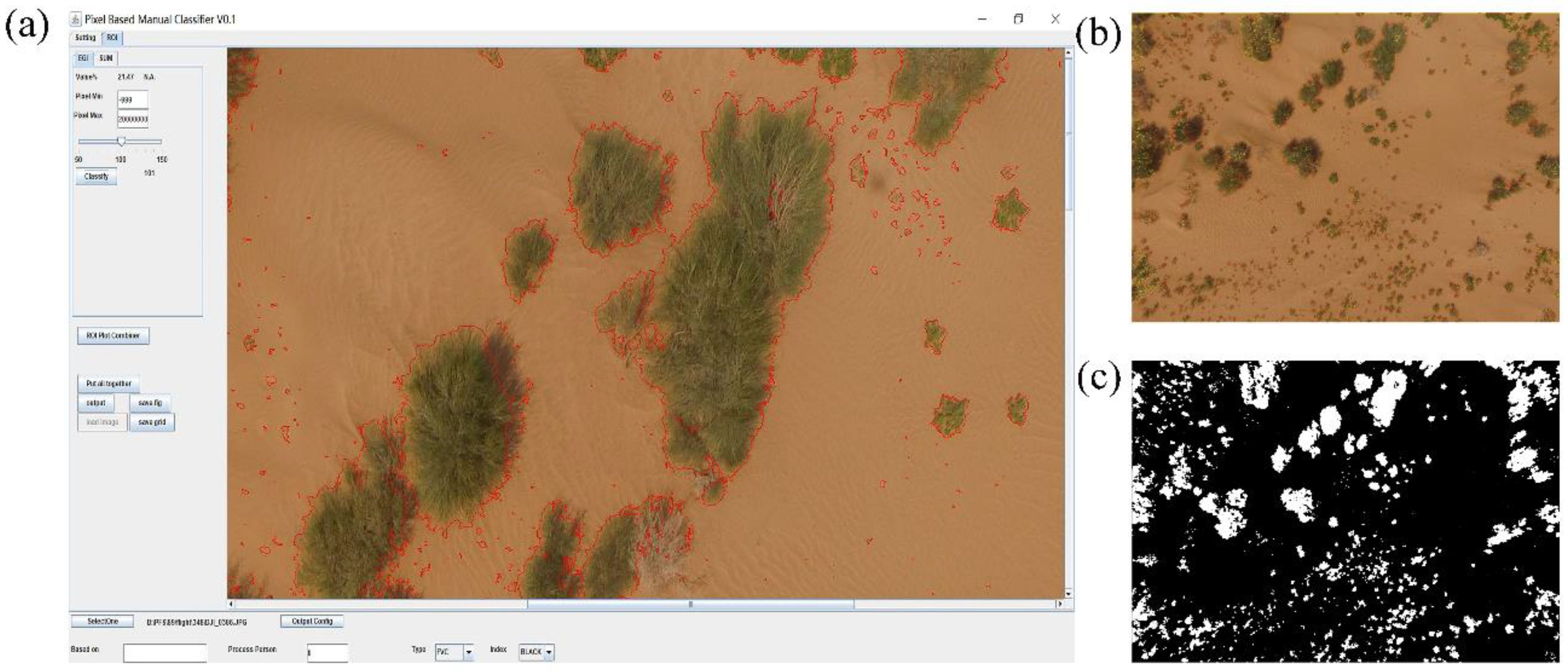
PixelClassifier software was adopted to extract the FVC of each photo, and the average FVC value of 16 photos was taken as the real FVC of each sampling plot. PixelClassifier software classifies images based on pixels (Figure 3). Pixels can be divided into vegetation and bare land based on a specified threshold. According to the enhanced green index (EGI), the optimal threshold was adjusted to distinguish vegetation from bare land. The value denotes the FVC. Optionally, before classification, a region of interest (ROI) could be selected and adjusted to the optimal threshold and could be applied for the entire photo. Based on the processed photos, classification map information was output as both text and pictures (Figure 3).
2.3.2. FVC Inversion Based on MODIS-NDVI Data
The dimidiate pixel model was used to invert FVC. The dimidiate pixel model assumes that a pixel includes both vegetation and soil. If the area occupied by vegetation in a pixel is fc, the area occupied by soil is 1 − fc, and the NDVI of the vegetation is NDVIV. The NDVI of the soil is NDVIS, and according to the linear mixing model of the pixels, the NDVI of the mixed pixels is expressed by Equation (1).
NDVI = fc × NDVIV+ (1 − fc) NDVIS.
According to Equation (1), FVC(fc) is obtained by Equation (2):
fc = (NDVI − NDVIS)/(NDVIV − NDVIS).
The values of NDVIV and NDVIS are very important when calculating FVC using the dimidiate pixel model. This article determined the values of NDVIV and NDVIS based on the 1% confidence interval of the cumulative frequency distribution of NDVI values in the image. The maximum value of the confidence interval represented NDVIV, and the minimum value of the confidence interval represented NDVIS. Finally, the values of NDVIV and NDVIS were determined to be 0.8125 and 0.0428, respectively.
2.4. Collection and Processing of Meteorological Data
Meteorological data included land surface temperature, temperature (air temperature), precipitation and evaporation, which were derived from China’s Integrated Meteorological Information Sharing System (http://cdc.nmic.cn). Land surface temperature and temperature were the annual averages of 2017, and precipitation and evaporation were the cumulative values of 2017. The data sets of 29 meteorological stations that covered the entire research area were sorted (Figure 1). Kriging interpolation was adopted to obtain the data of the entire study area, and the meteorological data for each sampling plot were extracted. Kriging interpolation, a method for spatial modelling and prediction of random fields based on covariance functions, has good interpolation effects on meteorological data and is often applied to process meteorological data [30].
2.5. Accuracy Verification
Both absolute and relative verification methods were introduced to verify the inversion results of vegetation coverages. The absolute verification compared the measured NDVI values obtained by the GreenSeeker handheld spectrometer with the NDVI values extracted by MODIS-NDVI data to verify the accuracy of MODIS-NDVI data for desert vegetation. The relative verification compared the FVC extracted from the aerial photographs with the FVC retrieved from the MODIS-NDVI image to verify the accuracy of the FVC inversion based on the dimidiate pixel model. In the analysis, the coefficient of determination (R2), root mean square error (RMSE), normalized root mean square error (NRMSE), and mean absolute error (MAE) were used as the basis of analysis. In this experiment, the NDVI measured by the GreenSeeker handheld spectrometer and the FVC extracted by the high-resolution photos taken by the UAV were regarded as the real values of desert vegetation of the study area.
2.6. Data Analysis
R was used to analyse the data [31,32,33]. Correlation and regression analyses were used to explore the relationship between FVC and longitude, latitude, altitude and meteorological elements, and to reveal the spatial distribution characteristics of vegetation coverage in the Alxa region. Stepwise regression analysis was used to analyse the change rule of FVC with meteorological factors, and a multivariate linear mixed model was used to reveal the relationship between these factors and to calculate the ratio of each meteorological factor in R2 of the regression model.
3. Results
3.1. Variation Characteristics of FVC, NDVI, and Meteorological Elements in Alxa
It can be seen from Table 1 that the NDVI values of 100 sampling points measured by the GreenSeeker handheld spectrometer (NDVIR) were between 0.0645 and 0.3980, with an average value of 0.1544 and a standard deviation of 0.0702, of which 67% of the samples had below the average and 79% of the samples had values less than 0.2. The NDVI values of samples extracted from MODIS-NDVI images (NDVIM) were between 0.0689 and 0.3906, with an average of 0.1591 and a standard deviation of 0.0745. The FVC values of the sample points extracted from the aerial photographs of the drone (FVCR) were between 0.0130 and 0.5354, the average value was 0.1573, the standard deviation was 0.1214, 63% of the sampling points had values below the average value, and 70% of the sampling points had values less than 0.2. The FVC values of the sample points inverted by MODIS-NDVI (FVCM) were between 0.0338 and 0.4503, with an average value of 0.1506 and a standard deviation of 0.0965. In Alxa, the average annual temperature was 9.51 °C, and the average annual temperature of 100 sampling points was between 8.39 and 10.49 °C. The average precipitation in this area was 168.55 mm, and the precipitation at the sampling point was between 93.31 and 325.95 mm: 62% of the sampling points had lower than average precipitation, and 79% of the sampling points had less than 200 mm. The annual average evaporation was 1790.41 mm, and the evaporation at the sampling points was between 1275.30 and 2203.54 mm. The evaporation of 54% of the sampling points was greater than the average, and 37% of the sampling had evaporation greater than 2000 mm. The average land surface temperature was 12.94 °C, the land surface temperature of each sampling point was between 11.36 and 13.84 °C, and 55% of the sampling points had lower than average annual land surface temperature (Table 1).
3.2. Impact of Scale on this Experiment
In this experiment, we used drones to collect images of different heights at the same point. The flying height of the UAV varied from 10 to 100 metres, and images were taken every 10 metres. Ten photos were collected at each sample point (Figure 4), and a total of 67 sample points were collected. Table 2 shows the size of the actual range of ground represented by the photos taken by the drone at different heights. The difference in vegetation coverage extracted from photos taken at different height was small, as shown in Figure 5a, and the coefficient of variation was between 0.015 and 0.394, with an average value of 0.1122. Figure 5b shows that the range (maximum minus minimum) of vegetation coverage extracted from photos taken at different heights was 0.0043 and 0.0563, with an average value of 0.0306. The variation in the coefficient of variation and range indicated that the FVC extracted from the selected sample points in this area was minimally affected by the scale.
3.3. Verifying the Accuracy of MODIS-NDVI Data and FVCM
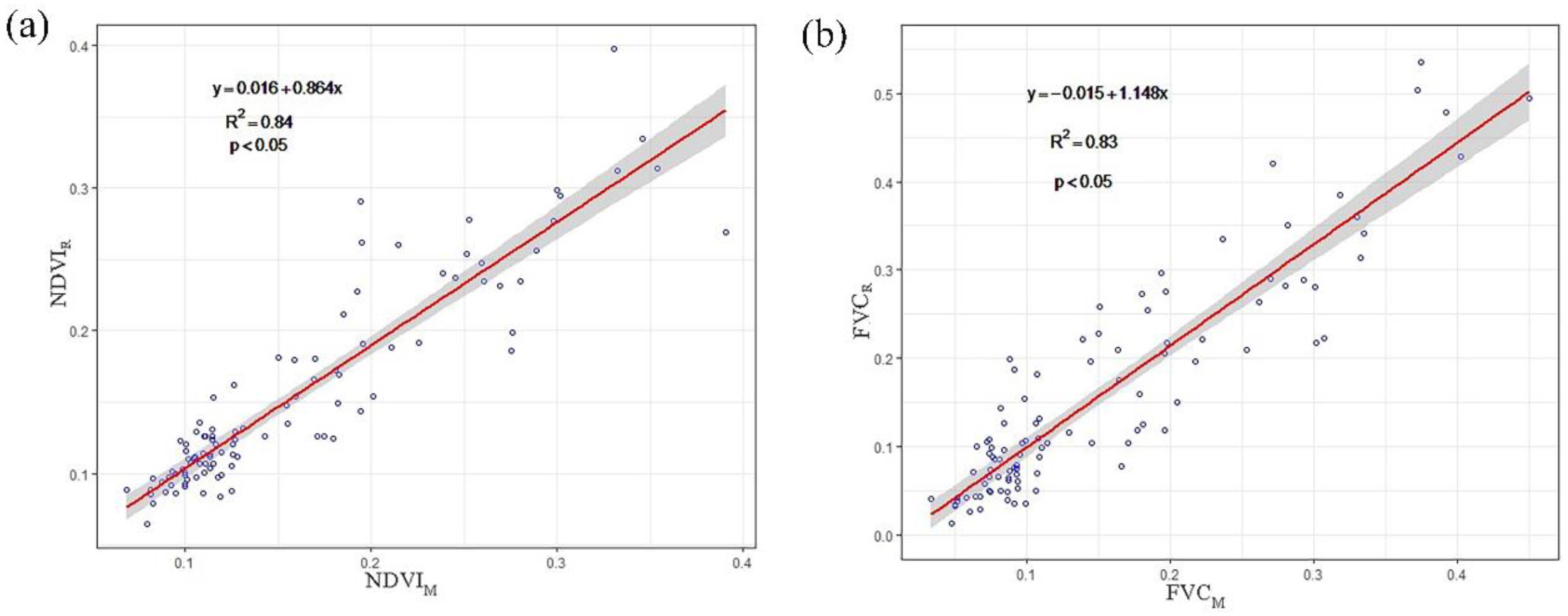
A correlation test was performed between NDVIR and NDVIM The results showed that there was a significant linear correlation between NDVIR and NDVIM, with a correlation coefficient of 0.92 (P < 0.001). Regression analysis indicated that NDVIM was slightly higher than NDVIR (Figure 6a): R2 of the regression equation was 0.84, the RMSE was 0.028, NRMSE was 42.57%, and MAE was −0.005 (Figure 6a). Correlation analysis was also performed between FVCR and the FVCM. The results showed a significant linear correlation between FVC values measured by GreenSeeker spectrometer (FVCR and FVCM, with a correlation coefficient of 0.91 (P < 0.001, Figure 6b). Regression analysis indicated that FVCM was slightly lower than FVCR: R2 of the regression equation was 0.83, the RMSE was 0.052, NRMSE was 42.94%, and MAE was 0.007 (Figure 6b).
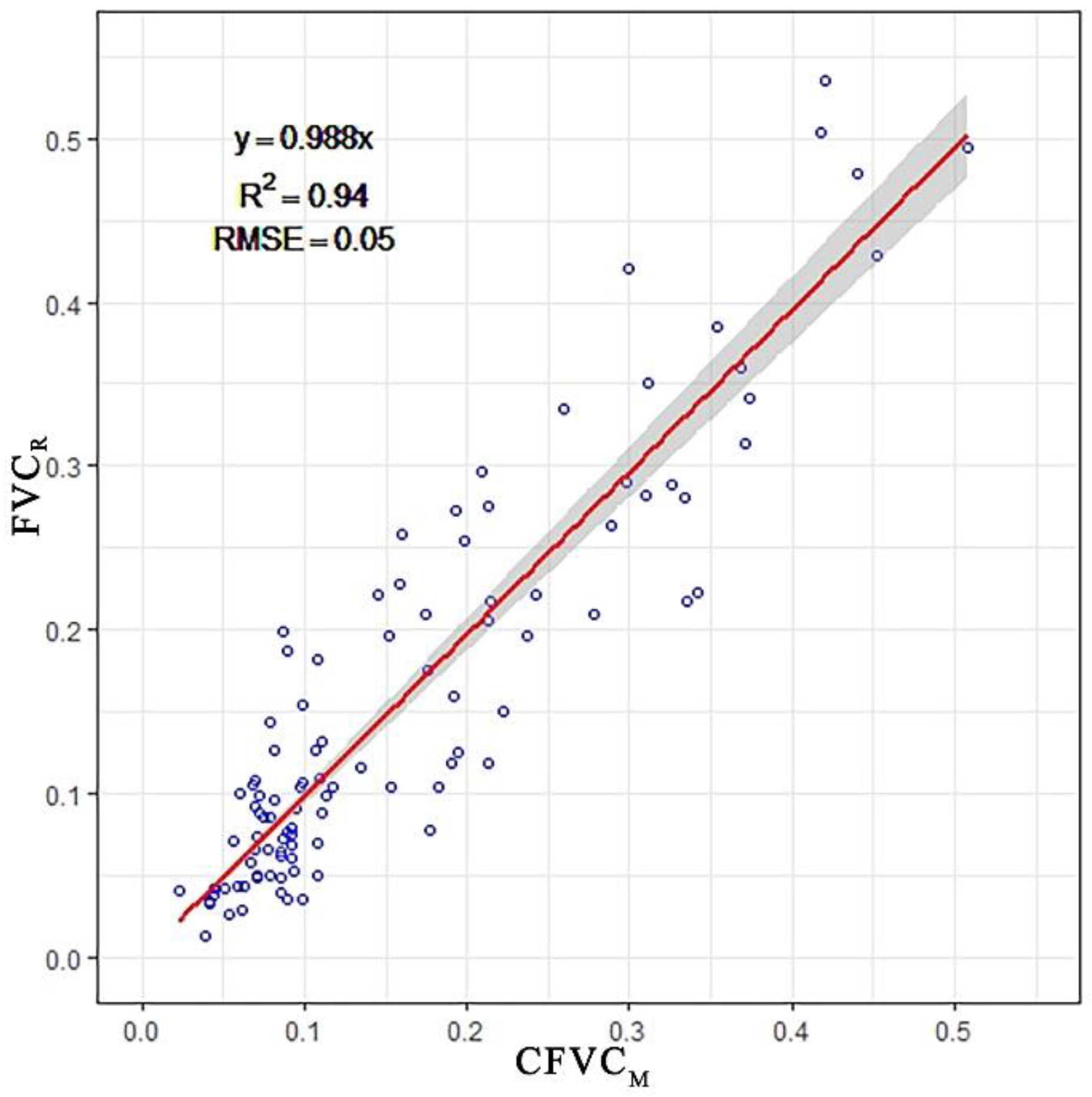
The MODIS-NDVI image was corrected using the linear regression equation of NDVIR and NDVIM and the abnormal pixels in the image were removed, then use the dimidiate pixel mode to invert the vegetation coverage (referred to as CFVCM). The maximum value in the image was regarded as NDVIV, the minimum value was regarded as NDVIS. As shown in Figure 7, after the MODIS-NDVI image was corrected, the intercept of the regression equations of CFVCM and FVCR was 0, indicating that the noise in the image had been eliminated, and the slope was 0.998, indicating that the inversion value can approximately replace the true value. The R2 of the regression equation was 0.94, which was 0.11 higher than that between FVCR and FVCM, the RMSE was 0.050, which was reduced by 0.002; the NRMSE was 40.96%, which was reduced by 1.98 %. Overall, the results were accurate when the corrected MODIS-NDVI image was used to retrieve FVC.
3.4. FVC Changes with Hydrothermal Gradient
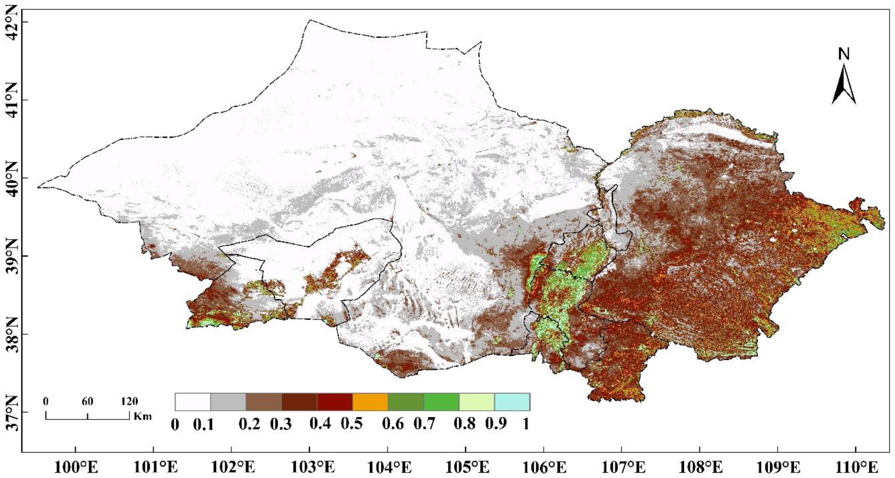
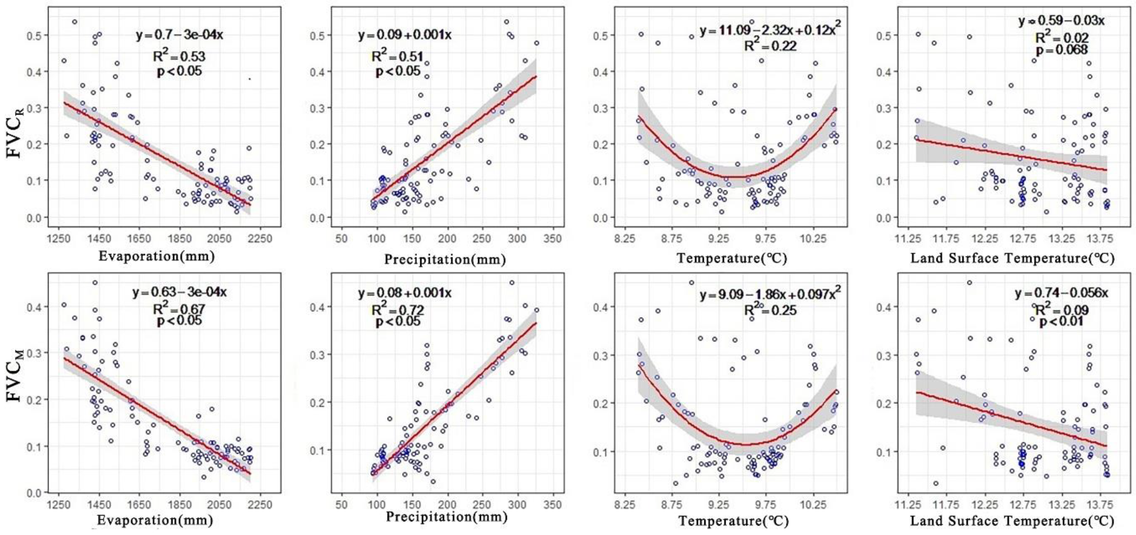
Figure 8 shows that the CFVCM gradually increased from north to south and from west to east. There was a significant negative correlation between FVC and evaporation, and both FVCM and FVCR had the same decreasing trend with increasing evaporation (Figure 9). FVC was significantly positively related to precipitation. The linear correlation between FVC and temperature was not significant, but regression analysis using a second-order polynomial found that FVC first decreased and then increased with rising temperature. Although there was a significant correlation between FVC and land surface temperature, the R2 value was small for the linear regression model, so it was believed that there was no linear correlation between land surface temperature and FVC. Stepwise regression analysis was used to analyse the relationship between FVC and various meteorological factors and the interactions among meteorological factors. The optimal regression fitting model of FVC was determined based on the R2, RMSE, NRMSE, and Akaike Information Criterion (AIC) of the model. According to the model, FVCR was affected by temperature, precipitation, and the interactions of evaporation vs land surface temperature, temperature vs land surface temperature, temperature vs precipitation, and temperature vs evaporation. The FVCM was affected by precipitation, evaporation, and the interactions of evaporation vs land surface temperature, and temperature vs land surface temperature (Table 3 and Table 4).
4. Discussion
4.1. Impact of Scale on This Experiment
The scale effect in remote sensing refers to the phenomenon that the analysis result changes as the spatial resolution of the remote sensing data changes. In this article, three spatial scale measurement tools are considered: the GreenSeeker handheld spectrometer, a UAV, and the MODIS satellite. When combining these three measurement tools to verify the vegetation coverage retrieved from satellite remote sensing data, spatial scale effects may lead to changes in the analysis results, including the applicability of the instrument, the underlying surface of the study area, and the model selection during the fusion of data of different scale. The GreenSeeker handheld spectrometer is an active sensor that measures the NDVI values of ground features and has been widely used in plant phenology observation [34], pest control [35,36], yield prediction [37] and nitrogen status detection [38]. GreenSeeker is often used as a tool for ground verification [39,40]. It has become a relatively mature technology in agriculture, but its application to desert grassland is rare. This article uses the GreenSeeker tool to correct MODIS-NDVI data products. The results show that this tool can effectively remove the noise in MODIS-NDVI data products, demonstrating the applicability of the GreenSeeker handheld spectrometer in desert grasslands. Another study found that the NDVI values extracted from low-spatial-resolution data are slightly lower than the real value, but the scale was a relatively minor contribution to this result [41], which is consistent with the results in this article. The NDVI values measured by the GreenSeeker handheld spectrometer were lower than the NDVI value extracted from MODIS-NDVI data products. At present, the extraction of vegetation coverage involves three main methods: ground measurement, satellite remote sensing technology, and UAV remote sensing technology. The accuracy is highest for UAV remote sensing technology [25]. This article also uses FVCR as the true FVC on the ground. In this test, we used the MODIS-NDVI data product, which is a three-level data product of MODIS, that has undergone radiometric calibration and atmospheric correction to eliminate data errors due to weather conditions, remote sensing platforms, sensors, etc. However, the terrain and environment of different regions are different, and the quality of the data is different. The spatial scale has little effect on MODIS remote sensing data products; Tian et al. [42] verified the inversion results of the MODIS data product LAI, and the results showed that MODIS LAI inversion results have a 5% error. In addition, studies have shown that when higher resolution data are aggregated into lower resolution data, the variation in the data will be reduced, and the effect of spatial heterogeneity will decrease, which could increase the correlation between FVC and the vegetation index (the red-edge normalization different water index, Green NDVI, enhanced vegetation index, NDVI) [26,43]. Therefore, the use of MODIS-NDVI data products with a spatial resolution of 250 m can not only meet the requirement that the image can cover the entire study area, but also effectively reduces the impact of spatial heterogeneity. Therefore, these three measurement tools of different scale can be used to verify vegetation coverage in desert grassland areas.
In terms of the scale effect, the conditions of the underlying surface in the study area including the features of the selected underlying surface, the relief of the terrain and other factors, often have a substantial impact on the results. For an underlying surface with large heterogeneity, a single point measurement or the average of a few points was used as the verification reference. There was a large uncertainty, but on a homogeneous and flat underlying surface, it may be appropriate to use several ground measurements in a pixel as the representative value of the pixel [44]. In this experiment, the terrain we selected was relatively low and flat, and Alxa is located in a temperate desert and arid region, with low vegetation coverage and few plant species. There are vast deserts in this area. The analysis results of the method of vertical shooting at a single point at different heights showed that the extraction of the vegetation coverage in this area is minimally affected by the scale. Therefore, it is appropriate to use the vegetation coverage extracted from the 16 photos taken by a drone over a 200 × 200 m area to represent the vegetation coverage in the 250 × 250 m space. The use of different models to fuse data at different spatial scales has a substational impact on the results. Some physical and mathematical models in a small area can be used to establish the relationship between the data at different spatial scales, and a statistical model (linear spectral mixture model) can be used on a large scale to establish an accurate vegetation spectral scale conversion relationship [45]. The establishment of statistical relationships between different scales of inversion values based on discrete images with different spatial resolutions can meet the needs when solving specific practical problems, but this approach cannot reflect the continuous scale conversion law of inversion values [46]. In this experiment, we used a simple linear regression model to establish the linear relationship between different scales, which not only effectively corrected the error of MODIS remote sensing data products, but also effectively verified the relationship between FVCU and FVCM. the results also confirmed that in desert grassland areas, the use of statistical models on a large scale can meet the requirement of practical problems.
4.2. The Influence of NDVI Image Data on the Inversion Results
When using the dimidiate pixel model to invert vegetation coverage, the characteristics of remote sensing data products, including the intrinsic quality of remote sensing data and the determination of NDVI values for pure bare land and pure vegetation, may impact the results. When the vegetation coverage exceeds 60%, the NDVI values tend to be saturated; that is, after the vegetation coverage reaches a certain threshold, the relationship between FVC and NDVI is no longer a simple linear relationship [47,48,49,50]. Therefore, the dimidiate pixel model may not to be suitable for inverting vegetation coverage in areas with high vegetation coverage. Among the sample points we investigated, the maximum FVC is 53.54%, the minimum is 1.3%, the average is 16.11%, and the FVC in most areas is below 20%; so there is no oversaturation of the NDVI values. Therefore, the dimidiate pixel model can be used to invert vegetation coverage in desert grassland areas. In addition, when the soil composition, soil particles, and water content in the pixel were changed, and the vegetation type and leaf water content were different, the pixel spectrum was different, and the NDVIS and NDVIV had greater uncertainty [51]. A series of research has studied how to determine the NDVIS and NDVIV [16,52,53]; for example, in a long-term sequence of remote sensing images, the minimum value of NDVI in a desert area was regarded as the NDVIS, and the maximum value in the image was used as the NDVIV [16]. Alternatively, these values have been determined based on percentiles of the image attribute value histogram [54]. Yang et al. [3] found an improvement to the traditional method for determining NDVIS, increased the RMSE of the FVC inversion results by 0.03. In areas with complex features, the determination of the NDVI values of pure bare land and pure vegetation pixels may be challenging, but in desert areas, the vegetation type is singular, and there are a large number of pixels without vegetation growth. NDVIV and NDVIS can be determined using the maximum and minimum values in the study area. However, MODIS-NDVI data have noise. The method used to determine the NDVI value of pure bare land and pure vegetation is to take the minimum and maximum values of the 1% confidence interval from the cumulative frequency table of the NDVI in the image. This method is suitable for desert areas. A regression relationship is established between the inversion value and the measured value. The coefficient of the regression equation indicates that the inversion value in this area is 14.80% lower than the measured value. For areas with scarce vegetation, if this inversion parameter is used for ecological value estimation, environmental carrying capacity evaluation, primary productivity evaluation, and scientific management, this error will affect the results and may affect the desert grassland management approach. In addition, some studies have shown that using the dimidiate pixel model to invert vegetation coverage will overestimate vegetation coverage [55]; this is inconsistent with our conclusion. We corrected the MODIS-NDVI data using the NDVI data collected on the ground. After eliminating data errors, the maximum and minimum values in the image were used as the NDVI values of pure vegetation and pure bare land; finally, the effect of noise in the original data was effectively reduced, and the accuracy of inversion was improved. Therefore, after removing the noise in the desert area data, the minimum and maximum values of the image can be used as the NDVI values for pure bare land and pure vegetation, which reveals the existence of errors in the MODIS-NDVI data product in desert areas; this may also be the main cause of underestimation. Use of the vegetation coverage retrieved by this product as the input parameter of a weather prediction model, regional or global climate change model, or global change monitoring model will cause errors in the results; therefore, MODIS-NDVI data products be calibrated before use.
4.3. The Effects of Meteorological Factors on Vegetation Coverage Obtained by Different Collection Methods
Plants play an important role in maintaining the energy balance of the surface. The structural characteristics of vegetation affect the exchange efficiency of energy and water, which will affect the regional climatic conditions. Changes in land surface vegetation coverage are among the important phenomena caused by regional climate change [56]. Studies have shown that temperature and precipitation are important factors affecting the spatial distribution of vegetation [57]. Li et al. [58] proved that precipitation was the most important factor affecting vegetation growth in northern China. FVCU was calculated from high-spatial-resolution images taken by UAV, and was regarded as the real FVC of each sampling plot. From the fitting equation and the contribution rate of each factor to the R2, it can be seen that the main meteorological factors affecting the Alxa area were precipitation, temperature and evaporation, but the interactions between land surface temperature and other meteorological factors also affects the FVCR. However, comparison of the two ways to obtain the polynomial regression model between FVC and the meteorological factors indicated that in the desert grassland area, because the vegetation has adapted the environment of high temperature and low rainfall, evaporation is not the main cause of the difference in the spatial distribution of vegetation, but it has a substantial impact on FVCM (R2V = 0.2357) (Table 4). One possible reason is that FVCM is obtained by inversion of MODIS-NDVI data. In contrast to UAV remote sensing, NDVIM is collected by MODIS satellite 705 km from the surface, and is greatly affected by the atmosphere. Moreover, NDVI is a physical parameter related to the red band and near-infrared band. Water vapour has a strong absorption band in the red and near-infrared regions. Evaporation affects the water vapour content in the atmosphere, resulting in the difference in measurement results. In desert regions, the interaction between temperature and evaporation, and the interaction between temperature and precipitation also impact the spatial distribution of vegetation, but they have no effect on FVCM. This finding is of great significance to studying of the relationship between FVC and meteorological factors, and reduces the complexity of data processing. Therefore, when exploring the relationship between vegetation coverage and meteorological elements, if vegetation coverage is retrieved from MODIS-NDVI data products or MODIS-NDVI data, when considering temperature and precipitation, the effect of evaporation should also be considered. However, this characteristic has been ignored in previous studies [57,58,59]. A polynomial regression model can be used to establish the relationship between meteorological elements and vegetation coverage. This also provides a new method for vegetation coverage prediction, especially for FVCM.
4.4. Impact of Human Disturbance on Vegetation Coverage
FVC was related to meteorological factors such as evaporation, precipitation, and temperature, however, the meteorological factors reflected the large-scale distribution characteristics of FVC, while the local differences could not be well expressed. Human activities such as land use/cover types, ecological restoration projects or management measures, and grazing disturbances also cause changes in FVC, resulting in obvious regional differences. Studies have shown that the disturbance of human activities has a substantial impact on FVC, and regional differences in FVC were also attributed to grazing intensity and livestock [60]. Therefore, it is inevitable that human activities affect the results of this experiment, and the choice of sample points is the most influential component. To minimize the influence of human interference factors on the test results, in the process of selecting samples, we chose plots that are least affected by human activities as the sample plots. However, the traces of human activities left over by history cannot be erased, so the influence of human activities still exists in the selected plots. How to effectively avoid the impact of these human activities on the test results requires further study.
5. Conclusions
The use of the original MODIS-NDVI data product with a spatial resolution of 250 m to invert vegetation coverage is practical in desert areas (R2 = 0.83, RMSE = 0.052, NRMSE = 42.94%, MAE = 0.007), but underestimated vegetation coverage in the study area. MODIS-NDVI data products are different from the real NDVI in the study area. Correcting MODIS-NDVI data products can improve the accuracy of inversion. When extracting vegetation coverage in this area, the scale has little effect on the results. There is a significant correlation between precipitation, evaporation and FVC, but the interaction of temperature and land surface temperature with precipitation and evaporation also have a considerable impact on FVC, and evaporation has a substantial impact on FVCM. When exploring the relationship between vegetation coverage and meteorological elements, if vegetation coverage retrieved from MODIS-NDVI data products or MODIS-NDVI data is used, when considering temperature and precipitation, the effect of evaporation should also be considered. In addition, meteorological factors can be used to predict FVC (R2 = 0.7364, RMSE = 0.0623), a new method for estimating FVC in areas with less manual intervention.
Author Contributions
Conceptualization, M.H.; methodology, L.T., M.H. and X.L.; software, L.T.; validation, M.H.; formal analysis, L.T.; investigation, L.T. and M.H.; resources, L.T. and M.H.; data curation, L.T.; writing—original draft preparation, L.T.; writing—review and editing, M.H. and X.L.; visualization, L.T.; supervision, L.T. and X.L.; project administration, M.H. and X.L.; funding acquisition, M.H. and X.L. All authors have read and agreed to the published version of the manuscript.
Funding
This work was supported by the Strategic Priority Research Program of the Chinese Academy of Sciences (No. XDA2003010301), Research and Development Funds of the Transport Bureau of Ningxia Hui Autonomous Region (WMKY1), and the National Natural Science Foundation of China (No. 41671103).
Acknowledgments
The authors would like to thank the financial support provided by the Strategic Priority Research Program of Chinese Academy of Sciences, and the Research and Development Funds of Transport Bureau of Ningxia Hui Autonomous Region, and the National Natural Science Foundation of China.
Conflicts of Interest
The authors declare no conflict of interest.
References
- Feng, L.L.; Jia, Z.Q.; Li, Q.X.; Zhao, A.Z.; Zhao, Y.L.; Zhang, Z.J. Spatiotemporal change of sparse vegetation coverage in northern China. J. Indian Soc. Remote Sens. 2019, 47, 359–366. [Google Scholar] [CrossRef]
- Schlesinger, W.H.; Pilmanis, A.M. Plant-soil interactions in deserts. Biogeochemistry 1998, 42, 169–187. [Google Scholar] [CrossRef]
- Iizuka, K.; Kato, T.; Silsigia, S.; Soufiningrum, A.Y.; Kozan, O. Estimating and examining the sensitivity of different vegetation indices to fractions of vegetation cover at different scaling grids for early stage acacia plantation forests using a fixed-wing UAS. Remote Sens. 2019, 11, 1816. [Google Scholar] [CrossRef] [Green Version]
- Baret, F.; Clevers, J.; Steven, M.D. The robustness of canopy gap fraction estimates from red and near-infrared reflectances – a comparison of approaches. Remote Sens. Environ. 1995, 54, 141–151. [Google Scholar] [CrossRef]
- Huete, A.R.; Tucker, C.J. Investigation of soil influences in AVHRR and near – infrared vegetation index imagery. Int. J. Remote Sens. 1991, 12, 1223–1242. [Google Scholar] [CrossRef]
- Parmesan, C.; Yohe, G. A globally coherent fingerprint of climate change impacts across natural systems. Nature 2003, 421, 37–42. [Google Scholar] [CrossRef]
- Myneni, R.B.; Keeling, C.D.; Tucker, C.J.; Asrar, G.; Nemani, R.R. Increased plant growth in the northern high latitudes from 1981 to 1991. Nature 1997, 386, 698–702. [Google Scholar] [CrossRef]
- Weltzin, J.F.; Loik, M.E.; Schwinning, S.; Williams, D.G.; Fay, P.A.; Haddad, B.M.; Harte, J.; Huxman, T.E.; Knapp, A.K.; Lin, G.H.; et al. Assessing the response of terrestrial ecosystems to potential changes in precipitation. Bioscience 2003, 53, 941–952. [Google Scholar] [CrossRef]
- Keeling, C.D.; Chin, J.F.S.; Whorf, T.P. Increased activity of northern vegetation inferred from atmospheric CO2 measurements. Nature 1996, 382, 146–149. [Google Scholar] [CrossRef]
- Curran, P.J.; Williamson, H.D. Sample size for ground and remotely sensed sata. Remote Sens. Environ. 1986, 20, 31–41. [Google Scholar] [CrossRef]
- Nemani, R.R.; Running, S.W.; Pielke, R.A.; Chase, T.N. Global vegetation cover changes from coarse resolution satellite data. J. Geophys. Res.-Atmos. 1996, 101, 7157–7162. [Google Scholar] [CrossRef] [Green Version]
- Okin, G.S.; Clarke, K.D.; Lewis, M.M. Comparison of methods for estimation of absolute vegetation and soil fractional cover using MODIS normalized BRDF-adjusted reflectance data. Remote Sens. Environ. 2013, 130, 266–279. [Google Scholar] [CrossRef] [Green Version]
- Xiao, Q.; Tao, J.; Xiao, Y.; Qian, F. Monitoring vegetation cover in Chongqing between 2001 and 2010 using remote sensing data. Environ. Monit. Assess. 2017, 189. [Google Scholar] [CrossRef] [PubMed]
- Gitelson, A.A. Remote estimation of crop fractional vegetation cover: The use of noise equivalent as an indicator of performance of vegetation indices. Int. J. Remote Sens. 2013, 34, 6054–6066. [Google Scholar] [CrossRef]
- Okin, G.S. Relative spectral mixture analysis—A multitemporal index of total vegetation cover. Remote Sens. Environ. 2007, 106, 467–479. [Google Scholar] [CrossRef]
- Gutman, G.; Ignatov, A. The derivation of the green vegetation fraction from NOAA/AVHRR data for use in numerical weather prediction models. Int. J. Remote Sens. 1998, 19, 1533–1543. [Google Scholar] [CrossRef]
- Atzberger, C.; Rembold, F. Mapping the spatial distribution of winter crops at sub-pixel level using AVHRR NDVI time series and neural nets. Remote Sens. 2013, 5, 1335–1354. [Google Scholar] [CrossRef] [Green Version]
- Tottrup, C.; Rasmussen, M.S.; Eklundh, L.; Jonsson, P. Mapping fractional forest cover across the highlands of mainland Southeast Asia using MODIS data and regression tree modelling. Int. J. Remote Sens. 2007, 28, 23–46. [Google Scholar] [CrossRef]
- Leprieur, C.; Kerr, Y.H.; Mastorchio, S.; Meunier, J.C. Monitoring vegetation cover across semi-arid regions: Comparison of remote observations from various scales. Int. J. Remote Sens. 2000, 21, 281–300. [Google Scholar] [CrossRef]
- Xiao, J.F.; Moody, A. A comparison of methods for estimating fractional green vegetation cover within a desert-to-upland transition zone in central New Mexico, USA. Remote Sens. Environ. 2005, 98, 237–250. [Google Scholar] [CrossRef]
- Turner, D.; Lucieer, A.; Watson, C. An automated technique for generating georectified mosaics from ultra-high resolution unmanned aerial vehicle (UAV) imagery, based on structure from motion (SfM) point clouds. Remote Sens. 2012, 4, 1392–1410. [Google Scholar] [CrossRef] [Green Version]
- Guo, Q.; Wu, F.; Hu, T.; Chen, L.; Liu, J.; Zhao, X.; Gao, S.; Pang, S. Perspectives and prospects of unmanned aerial vehicle in remote sensing monitoring of biodiversity. Biodivers. Sci. 2016, 24, 1267–1278. [Google Scholar] [CrossRef]
- Iizuka, K.; Yonehara, T.; Itoh, M.; Kosugi, Y. Estimating tree height and diameter at breast height (DBH) from digital surface models and orthophotos obtained with an unmanned aerial system for a Japanese cypress (chamaecyparis obtusa) forest. Remote Sens. 2018, 10, 13. [Google Scholar] [CrossRef] [Green Version]
- Fang, S.H.; Tang, W.C.; Peng, Y.; Gong, Y.; Dai, C.; Chai, R.H.; Liu, K. Remote estimation of vegetation fFraction and flower fraction in oilseed rape with unmanned aerial vehicle Data. Remote Sens. 2016, 8, 416. [Google Scholar] [CrossRef] [Green Version]
- Chen, J.; Yi, S.; Qin, Y.; Wang, X. Improving estimates of fractional vegetation cover based on UAV in alpine grassland on the Qinghai-Tibetan Plateau. Int. J. Remote Sens. 2016, 37, 1922–1936. [Google Scholar] [CrossRef]
- Riihimaki, H.; Luoto, M.; Heiskanen, J. Estimating fractional cover of tundra vegetation at multiple scales using unmanned aerial systems and optical satellite data. Remote Sens. Environ. 2019, 224, 119–132. [Google Scholar] [CrossRef]
- Ming-zhu, H.E.; Zhi-shan, Z.; Xiao-jun, L.I.; Rong-liang, J.I.A.; Jing-guang, Z.; Jing-gang, Z. Environmental effects on distribution and composition of desert vegetations in Alxa Plateau: Ⅰ. Environmental effects on the distribution patterns of vegetation in Alxa Plateau. J. Desert Res. 2010, 30, 46–56. [Google Scholar]
- Yi, S. FragMAP: A tool for long-term and cooperative monitoring and analysis of small-scale habitat fragmentation using an unmanned aerial vehicle. Int. J. Remote Sens. 2017, 38, 2686–2697. [Google Scholar] [CrossRef]
- Sun, Y.; Yi, S.; Hou, F. Unmanned aerial vehicle methods makes species composition monitoring easier in grasslands. Ecolog. Indic. 2018, 95, 825–830. [Google Scholar] [CrossRef]
- Junlong, L.I.; Jian, Z.; Cong, Z.; Quangong, C. Analyze and compare the spatial Interpolation methods for climate factor. Pratacultural Sci. 2006, 23, 6–11. [Google Scholar]
- John, F.; Sanford, W. An. {R} Companion to Applied Regression, 2nd ed.; Sage: Thousand Oaks, CA, USA, 2011. [Google Scholar]
- Venables, W.N.; Ripley, B.D. Modern Applied Statistics with S, 4th ed.; Springer: New York, NY, USA, 2002. [Google Scholar]
- Chris, W.R.; Ralph, M.N. Hier.part: Hierarchical Partitioning; R package version 1.0-4. Available online: https://CRAN.R-project.org/package=hier.part (accessed on 26 April 2020).
- Souza, H.B.; Baio, F.H.R.; Neves, D.C. Using passive and active multispectral sensors on the correlation with the phenological indices of cotton. Eng. Agric. 2017, 37, 782–789. [Google Scholar] [CrossRef] [Green Version]
- Zhang, G.L.; Tao, X.; Zhang, Z.; Du, Y.X.; Lu, X. Monitoring of Aphis gossypii Using Greenseeker and SPAD Meter. J. Indian Soc. Remote Sens. 2017, 45, 361–367. [Google Scholar] [CrossRef]
- Martin, D.E.; Latheef, M.A. Active optical sensor assessment of spider mite damage on greenhouse beans and cotton. Exp. Appl. Acarol. 2018, 74, 147–158. [Google Scholar] [CrossRef]
- Ji, R.T.; Min, J.; Wang, Y.; Cheng, H.; Zhang, H.L.; Shi, W.M. In-Season yield prediction of cabbage with a hand-held active canopy sensor. Sensors 2017, 17, 2287. [Google Scholar] [CrossRef] [Green Version]
- Ali, A.M.; Abou-Amer, I.; Ibrahim, S.M. Using GreenSeeker active optical sensor for optimizing maize nitrogen fertilization in calcareous soils of Egypt. Arch. Agron. Soil Sci. 2018, 64, 1083–1093. [Google Scholar] [CrossRef]
- Enciso, J.; Maeda, M.; Landivar, J.; Jung, J.; Chang, A. A ground based platform for high throughput phenotyping. Comput. Electron. Agricul. 2017, 141, 286–291. [Google Scholar] [CrossRef]
- Duan, T.; Chapman, S.C.; Guo, Y.; Zheng, B. Dynamic monitoring of NDVI in wheat agronomy and breeding trials using an unmanned aerial vehicle. Field Crop. Res. 2017, 210, 71–80. [Google Scholar] [CrossRef]
- Friedl, M.A.; Davis, F.W.; Michaelsen, J.; Moritz, M.A. Scaling and uncertainty in the relationship between the NDVI and land surface biophysical variables: An analysis using a scene simulation model and data from FIFE. Remote Sens. Environ. 1995, 54, 233–246. [Google Scholar] [CrossRef]
- Hu, Y.; Xu, Z.; Liu, Y.; Yan, Y. A Review of the Scaling Issues of Geospatial Data. Adv. Earth Sci. 2013, 28, 297–304. [Google Scholar]
- Dark, S.J.; Bram, D. The modifiable areal unit problem (MAUP) in physical geography. Prog. Phys. Geogr. 2007, 31, 471–479. [Google Scholar] [CrossRef] [Green Version]
- Snyder, W.C.; Wan, Z.M.; Zhang, Y.L.; Feng, Y.Z. Requirements for satellite land surface temperature validation using a silt playa. Remote Sens. Environ. 1997, 61, 279–289. [Google Scholar] [CrossRef]
- Huawei, W.A.N.; Jindi, W.; Yonghua, Q.U.; Ziti, J.; Hao, Z. Preliminary research on scale effect and scaling-up of the vegetation spectrum. J. Remote Sens. 2008, 12, 538–545. [Google Scholar]
- Luan, H.; Tian, Q.; Yu, T.; Hu, X.; Huang, Y.; Liu, L.; Du, L.; Wei, X. Review of up-scaling of quantitative remote sensing. Adv. Earth Sci. 2013, 28, 657–664. [Google Scholar]
- Huete, A.R.; Liu, H.Q.; Batchily, K.; van Leeuwen, W. A comparison of vegetation indices global set of TM images for EOS-MODIS. Remote Sens. Environ. 1997, 59, 440–451. [Google Scholar] [CrossRef]
- Huete, A.R.; Jackson, R.D.; Post, D.F. Spectral response of a plant canopy with different soil backgrounds. Remote Sens. Environ. 1985, 17, 37–53. [Google Scholar] [CrossRef]
- Diaz, B.M.; Blackburn, G.A. Remote sensing of mangrove biophysical properties: Evidence from a laboratory simulation of the possible effects of background variation on spectral vegetation indices. Int. J. Remote Sens. 2003, 24, 53–73. [Google Scholar] [CrossRef]
- Ding, Y.; Zheng, X.; Zhao, K.; Xin, X.; Liu, H. Quantifying the impact of NDVIsoil determination methods and NDVIsoil variability on the estimation of fractional vegetation cover in northeast China. Remote Sens. 2016, 8, 29. [Google Scholar] [CrossRef] [Green Version]
- Baumgardner, M.F.; Silva, L.F.; Biehl, L.L.; Stoner, E.R. Reflectance properties of soils. Adv. Agron. 1985, 38, 1–44. [Google Scholar]
- Johnson, B.; Tateishi, R.; Kobayashi, T. Remote sensing of fractional green vegetation cover using spatially-interpolated endmembers. Remote Sens. 2012, 4, 2619–2634. [Google Scholar] [CrossRef] [Green Version]
- Wu, D.H.; Wu, H.; Zhao, X.; Zhou, T.; Tang, B.J.; Zhao, W.Q.; Jia, K. Evaluation of spatiotemporal variations of global fractional vegetation cover based on GIMMS NDVI data from 1982 to 2011. Remote Sens. 2014, 6, 4217–4239. [Google Scholar] [CrossRef] [Green Version]
- Zeng, X.B.; Dickinson, R.E.; Walker, A.; Shaikh, M.; DeFries, R.S.; Qi, J.G. Derivation and evaluation of global 1-km fractional vegetation cover data for land modeling. J. Appl. Meteorol. 2000, 39, 826–839. [Google Scholar] [CrossRef]
- Jiang, Z.Y.; Huete, A.R.; Chen, J.; Chen, Y.H.; Li, J.; Yan, G.J.; Zhang, X.Y. Analysis of NDVI and scaled difference vegetation index retrievals of vegetation fraction. Remote Sens. Environ. 2006, 101, 366–378. [Google Scholar] [CrossRef]
- Chapin, F.S., III; Matson, P.A.; Vitousek, P. Principles of Terrestrial Ecosystem Ecology; Spring Science+Business Media. LLC: Berlin/Heidelberg, Germany, 2011. [Google Scholar]
- Li, C.; Wang, J.; Hu, R.; Yin, S.; Bao, Y.; Ayal, D.Y. Relationship between vegetation change and extreme climate indices on the Inner Mongolia Plateau, China, from 1982 to 2013. Ecolog. Indic. 2018, 89, 101–109. [Google Scholar] [CrossRef]
- Zhang, G.; Xu, X.; Zhou, C.; Zhang, H.; Ouyang, H. Responses of vegetation changes to climatic variations in Hulun Buir grassland in past 30 Years. Acta Geogr. Sin. 2011, 66, 47–58. [Google Scholar]
- Zhong, L.; Ma, Y.M.; Salama, M.S.; Su, Z.B. Assessment of vegetation dynamics and their response to variations in precipitation and temperature in the Tibetan Plateau. Clim. Change. 2010, 103, 519–535. [Google Scholar] [CrossRef]
- Sanaei, A.; Li, M.; Ali, A. Topography, grazing, and soil textures control over rangelands’ vegetation quantity and quality. Sci. Total Environ. 2019, 697. [Google Scholar] [CrossRef]
Figure 1.
Spatial distribution of sampling points and weather stations. Red dots and green dots are sampling points, where the green dots are also the points of spatial scale verification, and the blue dots are weather stations. To avoid the influence of human activities on the test results, we chose the plots that are less affected by human activities as the sampling plots; the sample area is flat, and the vegetation type is as simple as possible.

Figure 2.
Operation interfaces of unmanned aerial vehicle remote sensing (UAVRS) applications: (a) waypoint parameter setting in the FragMAP Locator APP which included the waypoint name, working point number, latitude, longitude, altitude, flight time, and weather conditions during the flight; (b) flight route setting in the FragMAP Monitor APP which provided functions of adjusting the space position of the route, setting the flight height, speed, overlap, and photo time of the route, and collecting the position information of each photo; and (c) the flight path.

Figure 3.
Operation interfaces of PixelClassifier. The threshold value ranges from 0 to 150, and the best classification result is determined according to visual discrimination. The threshold range in this classification process is 70–120. (a) Photo with a threshold of 101 that can achieve the best classification effect; the extracted vegetation coverage is 21.47%. The classification results are output in three forms: (b) colour map, (c) binary map in which white represents vegetation and black represents bare land, and text.

Figure 4.
Photos taken by drones at different heights.

Figure 5.
Impact of scale on extracting FVC: (a) the change in the coefficient of variation, and (b) the range of FVC extracted from 10 photos taken at 10–100 metres above each sample point.
Figure 5.
Impact of scale on extracting FVC: (a) the change in the coefficient of variation, and (b) the range of FVC extracted from 10 photos taken at 10–100 metres above each sample point.

Figure 6.
Linear relationships of (a) NDVIR and NDVIM, (b) and FVCR and FVCM.

Figure 7.
Linear relationships between FVCR and CFVCM.

Figure 8.
Spatial distribution of CFVCM in the study area. The colour bar shows the level of CFVCM divided into 10 levels at intervals of 0.1.
Figure 8.
Spatial distribution of CFVCM in the study area. The colour bar shows the level of CFVCM divided into 10 levels at intervals of 0.1.

Figure 9.
Relationship between FVC and meteorological factors.


Table 1.
Descriptive statistics of each element.
| Element | Range | Mean | Standard Deviation | Ration less than Average | Ratio below a Certain Threshold |
|---|---|---|---|---|---|
| NDVIR | 0.0645–0.3980 | 0.1544 | 0.0702 | 67% | 79% |
| NDVIM | 0.0689–0.3906 | 0.1591 | 0.0745 | 63% | 78% |
| FVCU | 0.0130–0.5354 | 0.1573 | 0.1214 | 63% | 70% |
| FVCM | 0.0338–0.4503 | 0.1506 | 0.0965 | 63% | 78% |
| Temperature (°C) | 8.39–10.49 | 9.51 | 0.54 | 43% | - |
| Precipitation (mm) | 93.31–325.95 | 168.55 | 59.58 | 62% | 79% |
| Evaporation (mm) | 1275.30–2203.54 | 1790.41 | 293.37 | 54% | 37% |
| Land surface temperature (°C ) | 11.36–13.84 | 12.94 | 0.66 | 55% | - |
Note: The threshold for NDVIR、NDVIM、FVCU、FVCM is 0.2, that for precipitation and Evaporation is 200 mm. (NDVI = normalized difference vegetation index, FVC = fractional vegetation coverage; NDVIR = NDVI values of sampling points measured by the GreenSeeker spectrometer; NDVIM = NDVI values of samples extracted from MODIS-NDVI images; FVC = fractional vegetation coverage; FVCU = FVC values from samples from photos taken by UAVs; FVCM = FVC values inverted from MODIS-NDVI data).
Table 2.
The size of the actual range of ground represented by the photos taken by the drone at different heights.
Table 2.
The size of the actual range of ground represented by the photos taken by the drone at different heights.
| Height(metres) | 10 | 20 | 30 | 40 | 50 | 60 | 70 | 80 | 90 | 100 |
|---|---|---|---|---|---|---|---|---|---|---|
| Length(metres) | 17.2 | 34.4 | 51.6 | 68.8 | 86 | 103.2 | 120.4 | 137.6 | 154.8 | 172 |
| Width(metres) | 12.8 | 25.6 | 38.4 | 51.2 | 64 | 76.8 | 89.6 | 102.4 | 115.2 | 128 |
Table 3.
The optimal fitting model between FVC and meteorological factors.
| Vegetation Index | Fitting Equation | R2 | RMSE | NRMSE | AIC |
|---|---|---|---|---|---|
| FVCR | FVCR = −10.53 + 1.939T + 0.01585P − 0.0003876T:V + 0.0002772V:L − 0.001559T:P − 0.06309T:L | 0.7364 | 0.0623 | 53.28% | −546.55 |
| FVCM | FVCM = −0.9219 − 0.002354V + 0.5962T + 0.001268P + 0.0001761V:L − 0.038T:L | 0.8342 | 0.0393 | 180.18% | −641.85 |
T, Temperature; P, Precipitation; L, Land Surface Temperature; V: Evaporation; “:”, Interaction.
Table 4.
The parts of each factor in R2 of the fitting equation.
| Vegetation Index | V | T | P | L | V:L | T:L | T:P | T:V | R2 |
|---|---|---|---|---|---|---|---|---|---|
| FVCR | - | 0.0429 | 0.1868 | - | 0.1500 | 0.0274 | 0.1999 | 0.1294 | 0.7364 |
| FVCM | 0.2357 | 0.0278 | 0.2991 | - | 0.2393 | 0.0323 | - | - | 0.8342 |
T = temperature; P = precipitation; L = land surface temperature; V = Evaporation; “:” = interaction.
© 2020 by the authors. Licensee MDPI, Basel, Switzerland. This article is an open access article distributed under the terms and conditions of the Creative Commons Attribution (CC BY) license (http://creativecommons.org/licenses/by/4.0/).
Share and Cite
MDPI and ACS Style
Tang, L.; He, M.; Li, X. Verification of Fractional Vegetation Coverage and NDVI of Desert Vegetation via UAVRS Technology. Remote Sens. 2020, 12, 1742. https://doi.org/10.3390/rs12111742
AMA Style
Tang L, He M, Li X. Verification of Fractional Vegetation Coverage and NDVI of Desert Vegetation via UAVRS Technology. Remote Sensing. 2020; 12(11):1742. https://doi.org/10.3390/rs12111742
Chicago/Turabian StyleTang, Liang, Mingzhu He, and Xinrong Li. 2020. "Verification of Fractional Vegetation Coverage and NDVI of Desert Vegetation via UAVRS Technology" Remote Sensing 12, no. 11: 1742. https://doi.org/10.3390/rs12111742
Note that from the first issue of 2016, this journal uses article numbers instead of page numbers. See further details here.