Challenges in UAS-Based TIR Imagery Processing: Image Alignment and Uncertainty Quantification


Geoinformation for Environmental Planning Lab, Technische Universität Berlin, Straße des 17. Juni 145, 10623 Berlin, Germany
*
Author to whom correspondence should be addressed.
Remote Sens. 2020, 12(10), 1552; https://doi.org/10.3390/rs12101552
Submission received: 3 April 2020
/
Revised: 10 May 2020
/
Accepted: 11 May 2020
/
Published: 13 May 2020
(This article belongs to the Section Remote Sensing Image Processing)
Abstract
:Thermal infrared measurements acquired with unmanned aerial systems (UAS) allow for high spatial resolution and flexibility in the time of image acquisition to assess ground surface temperature. Nevertheless, thermal infrared cameras mounted on UAS suffer from low radiometric accuracy as well as low image resolution and contrast hampering image alignment. Our analysis aims to determine the impact of the sun elevation angle (SEA), weather conditions, land cover, image contrast enhancement, geometric camera calibration, and inclusion of yaw angle information and generic and reference pre-selection methods on the point cloud and number of aligned images generated by Agisoft Metashape. We, therefore, use a total amount of 56 single data sets acquired on different days, times of day, weather conditions, and land cover types. Furthermore, we assess camera noise and the effect of temperature correction based on air temperature using features extracted by structure from motion. The study shows for the first time generalizable implications on thermal infrared image acquisitions and presents an approach to perform the analysis with a quality measure of inter-image sensor noise. Better image alignment is reached for conditions of high contrast such as clear weather conditions and high SEA. Alignment can be improved by applying a contrast enhancement and choosing both, reference and generic pre-selection. Grassland areas are best alignable, followed by cropland and forests. Geometric camera calibration hampers feature detection and matching. Temperature correction shows no effect on radiometric camera uncertainty. Based on a valid statistical analysis of the acquired data sets, we derive general suggestions for the planning of a successful field campaign as well as recommendations for a suitable preprocessing workflow.
1. Introduction
Land surface temperature is a key factor of ecological, cryospheric, and climatic systems [1]. Remote sensing systems that monitor the spatial distribution of ground surface temperature are used in a variety of fields such as agriculture [2], permafrost monitoring [3], soil moisture quantification [3,4], and urban studies [5,6].
Nevertheless, present satellite missions offering thermal data with high temporal resolution suffer from low spatial resolution (e.g., MODIS 1 km × 1 km). Smaller scale variations of 100–120 m can be observed by Landsat missions, but at very low temporal resolution (16 days). To assess small scale variations of land surface temperature at plant level and flexible temporal resolution, unmanned aerial systems (UAS, also referred as unmanned aerial vehicles (UAV)) as sensor platform are very promising and already in use to quantify plant water stress [7], canopy conductance [8], and turbulent heat fluxes [9,10].
In most cases, the UAS are equipped with thermal infrared (TIR) cameras sensitive to radiation in 5–14 m wavelengths [11]. Highest spatial resolution and radiometric accuracy are achieved with cooled TIR camera systems. Nevertheless, those are high in power consumption, weight, and cost. The more commonly used uncooled TIR cameras have a lower weight and consume less power while offering lower spatial resolution and measurement accuracy with manufacturer specifications of up to C.
The inaccuracy of uncooled TIR cameras is caused by the set-up of the sensor. The focal plane array (FPA) consists of uncooled microbolometers, which each function as single sensor elements. Those vary in sensitivity and offset depending on the FPA temperature and are not completely shielded against thermal radiation emitted by the camera interior, leading to a lower signal-to-noise ratio. Consequently, any temperature change in the camera interior, the FPA, or the lense causes temperature drifts in the measurements [12].
To reduce this effect, a common approach is to update the individual offset parameters of every microbolometer by imaging a surface of uniform temperature (shutter). This approach, also called nonuniformity correction (NUC), leads to a more homogenized response signal along the FPA. The shutter closes at specific time intervals or temperature changes. If the shutter frequency is too low, a temperature drift due to environmental changes during the image acquisition period can be observed [8,13,14]. Additionally, Berni et al. [8] and Kelly et al. [13] observe a stabilization of the measured values of different cameras up to 30 min after turning the camera on. Therefore, they propose a preheating of the system before image acquisition to avoid thermal drift caused by the destabilized temperature of the camera operating system. Kelly et al. [13] further recommend a windshield around the camera and a short time interval between shutter activation. Externally heated shutter systems that combine these requirements by performing the NUC based on a shutter surface heated to uniform temperatures outside of the whole camera system within an extra box around camera and lens are recently becoming available.
In the case of existing temperature drift in image data, Mesas-Carrascosa et al. [14] make use of identical points extracted by feature detection and matching algorithms to eliminate this effect. Maes et al. [15] proposed a correction by subtracting air temperature anomalies that were recorded during the flight time by a meteorological station from the imagery to reduce the influence of micro-climate changes during image acquisition. The effect of the temperature correction proposed by Maes et al. [15] on the accuracy of the camera has, to the best of our knowledge, never been analyzed.
Most studies dealing with radiometric image preprocessing aim for exact measurements of the ground surface temperature [13,16,17]. When aiming for exact ground surface temperatures, temperature control plates [7,13] or additional thermal sensors [14,16,18] are used for on-ground measurements. This leads to higher costs and further workload in fieldwork. Statistical and machine learning approaches do not necessarily require exact ground surface temperatures, but rather consistent relative temperature as valid data input. For those purposes, the noise of the sensor needs to be quantified to get impressions on the measurement stability of the cameras and the need for necessary corrections. As measurement stability can vary with each image acquisition [13,17], camera noise quantification needs to be performed for each flight campaign individually. An adaption of the approach presented by Mesas-Carrascosa et al. [14] has the potential to fulfil this requirement without additional fieldwork.
Besides radiometric accuracy, spatial analysis of ground surface temperature requires the single acquired image frames to be merged as an orthomosaic. The creation of orthomosaics relies on structure from motion (SfM) algorithms used in common mosaicking software (e.g., Pix4D and Agisoft). The basis of these algorithms is the detection and pairing of outstanding features between the different images [19]. In the case of a limited number of matching points, the orientation and geometric calibration of the camera can be imperfect. The low amount of information within the TIR compared to RGB pictures impedes the recognition of these features. TIR cameras supply only a single band with a very low image resolution (e.g., 0.09 MP Flir TAU 2 336) compared to RGB imagery (e.g., 18–50.6 MP Canon EOS series [20]). The low amount of information in TIR imagery is also reflected in the low contrast of the data. Several studies mention problems in image alignment potentially due to missing contrast among and within the images especially when capturing images at early morning hours [9,21,22]. Maes et al. [15] further state the dependency of alignment quality on land cover types, reporting difficulties when aligning images acquired over areas with complex canopy structure and very homogeneous grassland.
To overcome poor image alignment due to low contrast, Ribeiro-Gomes et al. [17] applied a Wallis filter [23] to increase the contrast in their images, showing a higher number of tiepoints found by the SfM algorithm and better image alignment. For the creation of the final orthomosaic, they exchanged the aligned filtered images with the unfiltered images. Brad [24] adapted the Wallis filter for satellite imagery, leading to even higher image contrast and better image enhancement.
The flight acquisition itself can also improve image alignment: A high horizontal and vertical overlap of the acquired images increases the area of possible matching point detection. Some applications underscore the benefit of an integrated RGB or multispectral camera to estimate the UAS position at the time of TIR image take for alignment of TIR imagery [15,25]. Nevertheless, not all studies use RGB or multispectral cameras on the same UAS. Additionally, the trigger time of the two cameras may not necessarily be the same.
For the generation of geometrically accurate imagery, a geometric camera calibration is necessary to take distortion parameters into account [26]. A common approach estimates the camera distortion coefficients from TIR imagery taken of a flat surface with regular patterns at close range. The estimated parameters are then included in the alignment process [9,15]. Maes et al. [15] found a slight increase in image alignment quality when applying geometric camera calibration parameters of this pre-calibration procedure to the alignment process. Nevertheless, Harwin et al. [27] showed that for RGB imagery the accuracy of the point cloud is the same or higher when geometric camera calibration parameters are estimated by Photoscan Agisoft during bundle adjustment instead of using pre-calibration parameters.
As described above, there are a variety of preprocessing challenges, ranging from camera settings, data acquisition date and time, image alignment properties, and relative thermal measurement stability varying for different land cover types. All of these issues have been described separately, but never in a larger study addressing the complexity and interrelation of the preprocessing steps. To overcome these uncertainties, as well as to prove hypotheses of previous studies, we analyse the impact of contrast enhancement and its parametrization, sun elevation angle, and land cover on image alignment for more than 50 flights. Furthermore, we provide insights on the possibilities to improve image alignment using common software by including information on yaw, pitch, and roll angle; geometric camera coefficients; or feature matching pre-selection methods.
As a result, this study can provide useful suggestions for a workflow of data acquisition and preprocessing as well as a method to quantify the noise of the sensor for campaigns that can be utilized without exact ground surface temperature. This approach will be used to analyze the benefit of a temperature correction following Maes et al. [15].
2. Materials and Methods
2.1. Study Sites
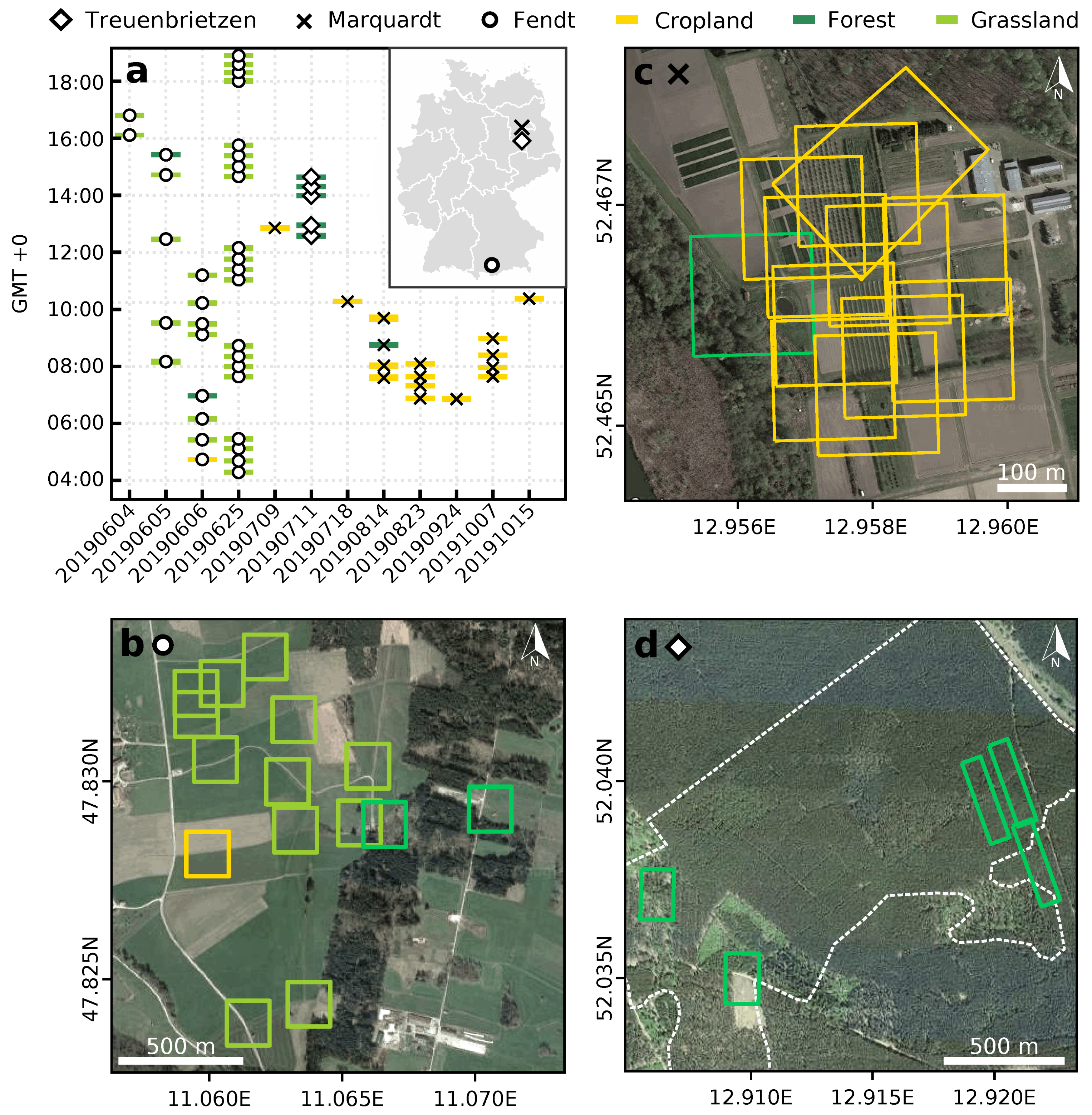
The UAS campaigns were performed at three different main study sites as displayed in Figure 1. Treuenbrietzen, located southwest of Berlin, Brandenburg, Germany, is a site affected by forest fires in 2018. The areas of interest include severely burnt pine plantations and clear cuts in the northwest, as well as mixed forests affected by lower fire severity in the east. Cumulus clouds (CC) were present during all flights.
Dominated by grassland and meadows, the pre-alpine catchment Fendt south of Munich, Bavaria, Germany, served as a second site. Two flight polygons also cover parts of the intersecting mixed forest. The site is part of the TERENO Pre-Alpine Observatory [28] and equipped with meteorological instruments.
Marquardt is a research station of the Leibniz Institute for Agricultural Engineering and Bioeconomy, located northwest of Potsdam, Brandenburg, Germany. Therefore, a variety of annual and perennial crops, such as cherry, walnuts, blueberry, corn, or wheat, is intersected by lean grassland or bare soil in fragmented patches. No meteorological background data with sufficient temporal resolution was available for Treuenbrietzen or Marquardt.
2.2. Image Acquisition
TIR imagery was acquired at 100 m altitude over different land cover types, sun elevation angle (SEA), and weather conditions. The time, date, site, and land cover type of every flight is summarized in Figure 1.
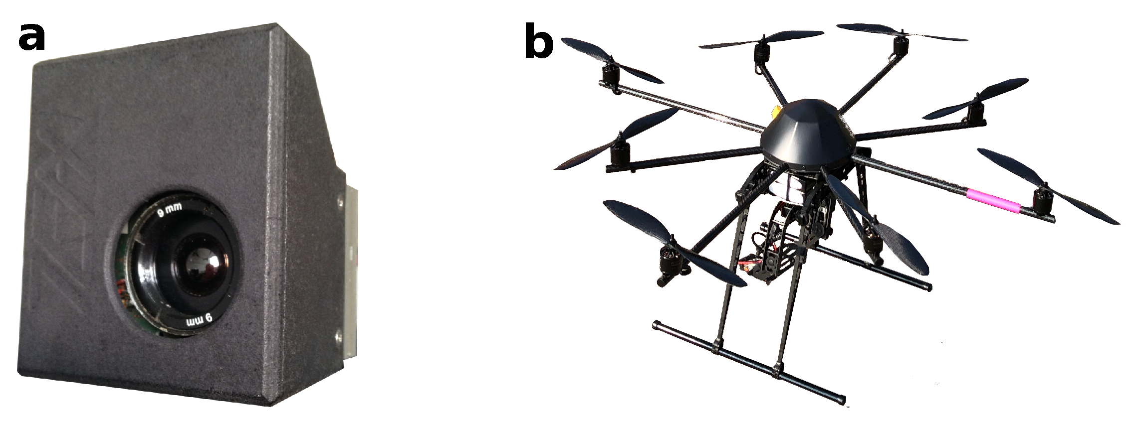
For the data acquisition, the UAS MK Okto XL 6S12 (HiSystems GmbH, Moormerland, Germany, Figure 2b) equipped with a radiometric calibrated FLIR Tau 2 336 (FLIR Systems, Inc., Wilsonville, OR, USA, Figure 2a) was used. This TIR camera uses an uncooled VOx microbolometer focal plane array which is sensitive to wavelengths from 7.5 to 13.5 m. Manufacturers specify an accuracy of C. The camera was upgraded with an external heated shutter system (TeAx Technology UG, Wilnsdorf, Germany) to achieve a better radiometric accuracy and avoid the vignetting effect [29] in the individual scenes (personal communication R. Schlepphorst 20 May 2019). Further features are its 9 mm focal length, a sensor resolution of 336 pixels × 256 pixels and a 35 27 field of view leading to a ground pixel size of 36 cm × 42 cm with 100 m flight altitude.
We preheated the camera before the flight for 10 min to 30 min on the ground to avoid thermal drift due to the stabilization of the camera system temperature, corresponding to Kelly et al. [13] and Berni et al. [16]. Flights were acquired at a speed of approximately 5 m/s, a nadir view angle, and a scene overlap of 82% × 84%. To ensure the specified overlap of the scenes, the trigger was automatically activated every 9 m. A gimbal (MK HiSight SLR2, HiSystems GmbH, Moormerland, Germany) ensured a steady nadir viewing angle. The acquisition time of all flights ranged between 11 and 13 min. The position and yaw angle of the vehicle at every acquisition event was recorded by a UBlox NEO-M8N GPS and compass module (u-blox Holding AG, Thalwil, Switzerland). In total, 56 flights are included in the data set.
2.3. Geometric Camera Calibration
For geometric camera calibration, a checkerboard was printed on a DinA3 paper. Black and white paper only differs marginally in the long wave infrared spectrum [30]. Therefore, we increased the contrast of the pattern by covering the white squares with aluminum foil, making use of the different emissivities of the two materials [30]. Images were taken of this checkerboard from different viewing angles as described in the Agisoft lens manual [31] at full sunlight conditions outside of buildings (from 11:20 h to 15:10 h UTC+2 on 12 August 2019, air temperature at 2 m: 21–22 C [32]). The images were then inserted to Agisoft lens tool (Agisoft Metashape Professional, version 1.5.3, Agisoft LLC, Petersburg, Russia) to estimate the 13 lens parameters (see estimated coefficients in Table A1).
2.4. Image Preprocessing
Three steps of data preprocessing were performed before the analysis of image alignment:
- For each individual image capture, the camera creates multiple frames. The frame with highest image quality according to the Agisoft Image Quality tool was selected for further processing to reduce the probability of blurry images. This tool aims to give an impression of image quality by returning a parameter that reflects the level of sharpness of the most focused part of the image [31].
- The extracted frames were temperature corrected, as proposed by Maes et al. [15], for flights performed in Fendt where sufficient meteorological background data were available,where and are the corrected and uncorrected measured temperature by the camera, respectively; is the air temperature at the moment of image capture; and is the mean of the air temperature during the flight. Air temperature of the local weather station with temporal resolution of 1 min served as input for the correction.
- We applied a contrast enhancement (CE) using the adapted Wallis filter of Brad [24] to the images. We chose a window size of 17 based on a pre-analysis for the local statistics calculation. We then tested different parameter settings based on the proposed range in Brad [24] of the edge enhancement factor A and uniform enhancement factor B. The chosen parameter combinations are listed in Table 1.
To analyze the benefit of GPS background information on the image alignment, we assigned the corresponding GPS position and yaw angle to every image using ExifTool (Phil Harvey, Kingston, Canada). Roll and pitch angle are 0 due to the steady nadir look angle provided by the gimbal.
2.5. Image Alignment Analysis
The analysis of image alignment quality was also performed in Agisoft Metashape, as it showed best performance in spatial accuracy [33] and image alignment [34]. Furthermore, related studies used this software for the analysis of best preprocessing practices of TIR imagery [13,15,17]. Agisoft provides several methods to search for possible matching points, e.g., generic pre-selection, reference pre-selection, or no pre-selection. In “Generic” mode, overlapping pairs of the image are defined using a downscaled resolution image first, whereas “Reference” mode selects overlapping pairs based on the image location supplied by its metadata [31].
Additionally, it is possible to include GPS background information such as yaw, pitch and roll angle. When the Reference pre-selection method is not selected, no GPS information is included in the feature matching process.
We also tested two geometric camera calibration methods: Estimating the camera calibration parameters as described in Section 2.3 (hereafter referred to as “calibrated”) or “on-job” during the bundle adjustment (hereafter referred to as “on-job”). These options in image preprocessing and combinations to define the bundle adjustment algorithm led to the combinations as listed in Table 1.
Data acquisitions took place at differing cloud cover conditions. Therefore, images acquired under dense cloud conditions are excluded from the analysis of land cover, combinations in Agisoft, and the effect of contrast enhancement.
For the analysis of the effect of SEA and weather conditions, we use the whole data set. In a second step, we concentrate on Grassland areas which are covered five times on the 25th of June to gain better insights on the effect of SEA alone. SEA and solar azimuth angles (SAA) were calculated using the NOAA Solar Calculator [35].
To analyze the impact of land cover on the image alignment, we defined three different land cover types: Areas with more than 50% forest area are assigned to the “Forest” land cover class. This class was composed mainly of flights performed at Treuenbrietzen. The “Cropland” class contains areas covered by annual and permanent crops, which is the case in Marquardt and one area of Fendt. “Grassland” only exists in Fendt and describes areas used as meadows or grassland. Example images for every landcover class are supplied in Figure A3.
To be able to compare the image alignment quality, the number of tiepoints and the number of aligned photos after every alignment run were used. The selection of these parameters is based on the results of Wierzbicki et al. [36], who showed that a higher density of the point clouds improves the spatial accuracy of the mosaicking results. Furthermore, those indicators are also used by other studies assessing alignment quality [15,17]. As they vary with every alignment, every setting (Table 1) was aligned ten times. Before extracting the number of points in the point cloud and aligned photos, we filtered the point cloud: Only points with a Reconstruction Uncertainty smaller than 20 and a Reprojection Error smaller than 0.5 were selected in order to extract only valid points.
As every campaign has a different number of images, normalization was required for valid comparison. We, therefore, chose the following equation with and being the number of points and aligned images, respectively, as returned by the Agisoft image alignment procedure.
Within the defined flight polygon, the camera automatically acquired images at a specified distance to fulfill overlap requirements. This was also the case during ascend and descend of the vehicle. As the flight height is not the same for those images, they are often not aligned. Those images were not excluded from the image alignment procedure for the sake of automatization. To include their effect on , Equation (2) is adapted to
with as the number of all images of the flight and as the number of images acquired during the way to and back from the flight polygon. With this, all the points are normalized to the number of images that should be theoretically alignable.
2.6. Camera Uncertainty Quantification
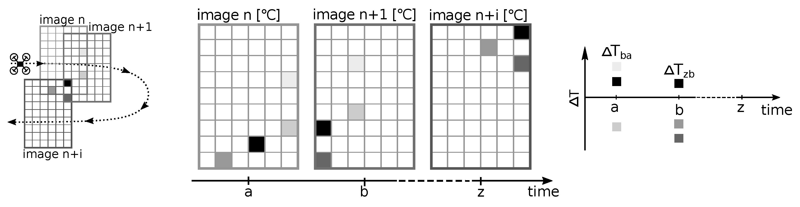
To assess the measurement noise of the camera, we adapted the basic idea of Mesas-Carrascosa et al. [14]. We used the SfM algorithms to detect features that occur on several images, applying the best combination of parameters in image preprocessing and in Agisoft. Those tiepoints were filtered to a Reconstruction Uncertainty lower than 15 and Reprojection Error lower than 3 when image alignment was successful. The positions of the remaining tiepoints were used to extract the temperature of this feature in overlapping images. We were now able to see the temporal development of differences in measured surfaces of identical features. We analyzed short-term fluctuations (temperature change of features in consecutive images with a maximum 4 s difference in acquisition time) and long-term differences (temperature change of features in images of adjacent flight paths with minimum 50 s difference in acquisition time) to detect systematic long-term temperature trends and short-term sensor noise. The applied image acquisition mode led to up to three to four consecutive images to be included in the uncertainty estimation for short-term and long-term noise, respectively. The presence of several tiepoints per image allowed for the derivation of standard descriptive statistics per time of image acquisition (see schematic procedure in Figure 3). This procedure enabled the detection of images with high noise and their removal from the orthomosaic to obtain radiometrically accurate imagery.
The above proposed method of uncertainty assessment allowed us to analyze the radiometric benefit of temperature correction as suggested by Maes et al. [15]. We described short-term and long-term noise with basic statistical parameters such as standard deviation, minimum, maximum, mean, and median for all flights processed with and without temperature correction. This analysis was only possible for areas in Fendt as meteorological data was only available there. As the extraction of tiepoints is based on successful image alignment, only aligned images could be used for tiepoint extraction. This led to a statistical analysis of 33 flights for the analysis of the temperature correction impact on camera noise.
3. Results
3.1. Impact of Image Preprocessing, IMU Data Inclusion, Geometric Camera Pre-Calibration, and Pre-Selection Options
Different options for direct preprocessing of the images when aligning them may strongly influence the quality of the final product, independent of external influences as land cover, weather conditions, or temporal effects. Therefore, these influences were analyzed first.
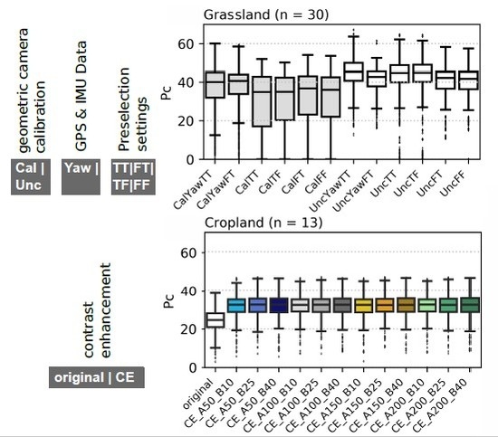
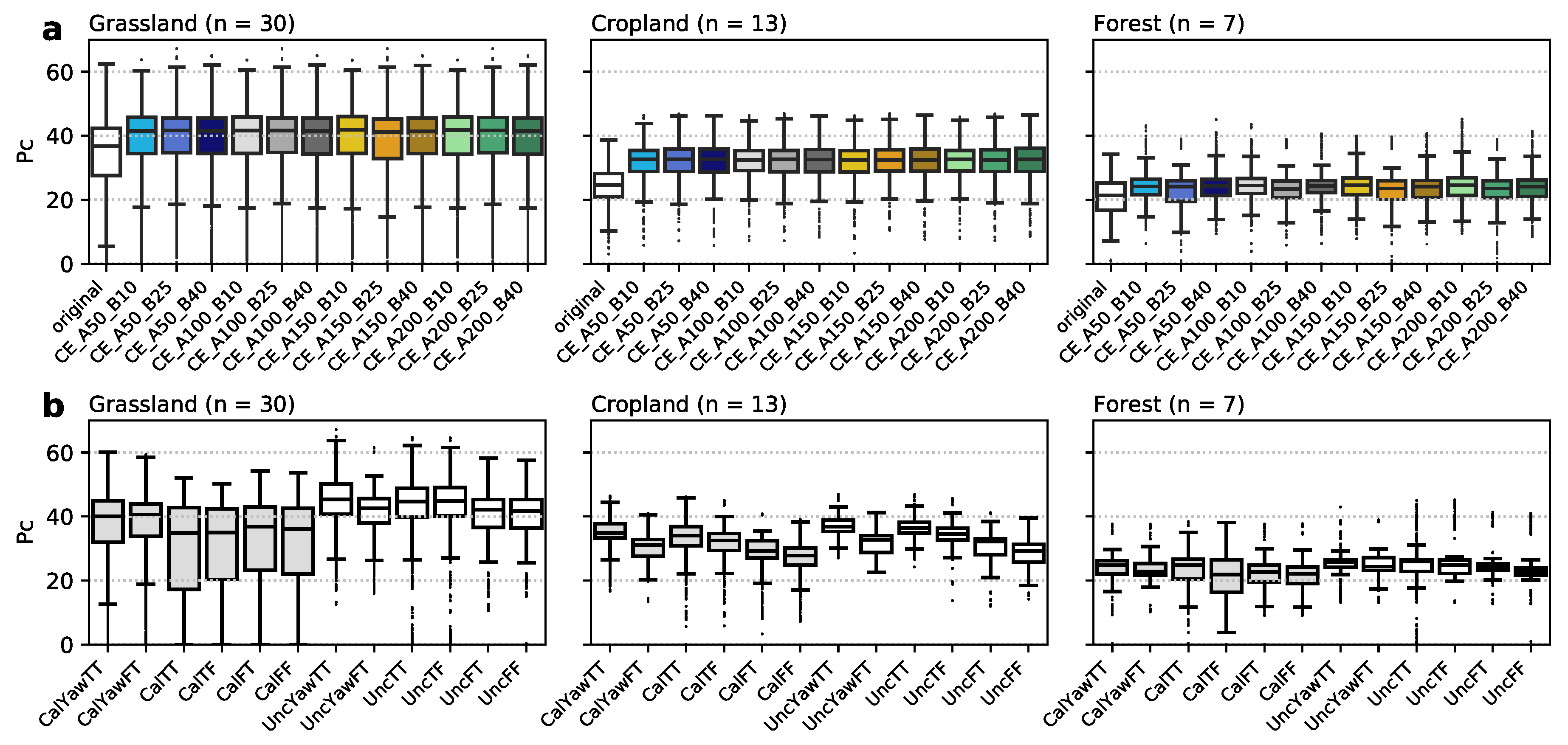
Figure 4a shows for different land cover classes and parametrizations of contrast enhancement for edge enhancement factor (A) and uniform enhancement factor (B) (e.g., CE_A50_B10: contrast enhancement with edge enhancement factor 50 and uniform enhancement 10, see further abbreviations in Table 1). The effect of contrast enhancement is clearly visible for all land cover classes. On average, filtering the images increases by 12.93%, 34%, and 11.99% for Grassland, Cropland, and Forest, respectively. Thereby, the effect of contrast enhancement is highest in Cropland and lowest for forested areas. For both, A and B, we are not able to define optimal parameters in the chosen range.
To avoid the distortion of the analysis due to the significantly lower for unfiltered images, we excluded this data from the continuing analysis. As among the different parameters only minor differences exist, we included all contrast enhanced data in the analysis of pre-selection methods and camera or image metadata (Figure 4b).
The reduced data set reveals the benefit of on-job geometric camera calibration, which is performed during the bundle adjustment. Applying estimates of camera coefficients derived from a pre-calibration for the image alignment reduces by 22.5%, 6.7%, and 7.3% for Grassland, Cropland, and Forest, respectively. Besides the reduction in , Figure 4b reveals an increasing instability in alignment reflected by high interquartile ranges (IQR) for pre-calibrated geometric camera coefficients when comparing corresponding settings. This is particularly prominent for Grassland areas with no orientation metadata included and both pre-selection methods selected (CalTT vs. UncTT, for abbreviations see Table 1). The standard deviation in the case of CalTT with 15.7 is nearly double the value of UncTT with a standard deviation of 9.2.
The inclusion of camera orientation angles has only a minor impact on camera alignment. The distribution of the data indicates a minor shift towards a higher and lower IQR, but no significant differences can be determined from this analysis.
Pre-selection in Agisoft, on the other hand, shows pronounced impact on image alignment. All land cover classes reflect the same pattern of decrease of when deselecting generic pre-selection for on-job geometrically calibrated cameras. This is very pronounced in Cropland areas. Thereby, the effect of generic pre-selection with a mean decrease of 2.7 for all land cover classes is higher than that of reference pre-selection (mean decrease of 0.6 for all land cover classes) for on-job camera coefficient estimation. The lowest effect between different combinations is again shown for the Forest land cover class.
The lowest values occur when matching features are not pre-filtered for potentially overlapping areas, whereas defining the matching area of the features by two methods shows best results.
Based on these results, the best settings are UncYawTT or UncTT for all land cover classes. We, therefore, analyzed the effect of land cover on image alignment based on the UncYawTT combination and the effect of weather conditions with CalTT, CalYawTT, UncTT, and UncYawTT, separately.
3.2. Influence of Land Cover
Land cover seems to have a large influence in the preprocessing quality of TIR imagery. Figure 4a,b reveals significant differences in for land cover types with Grassland areas having highest , followed by Cropland and Forest areas. The IQR when including all combinations in Agisoft (Figure 4a) is highest for Grassland with a high number of outliers and lowest for Forest areas. Nevertheless, the analysis of the impact of geometrical camera calibration clarifies the origin of the high range of of Grassland in Figure 4b. The geometrically pre-calibrated camera coefficients cause a more than doubled IQR compared to on-job geometrically calibrated cameras. When no distinction is made between the contrast enhancement parameters, geometric camera calibration methods, pre-selection methods, and weather, the mean value of for Grassland is 21.66% and 65% higher than the mean value for Cropland and Forest, respectively. This difference of in Grassland to of Cropland and Forest is further enhanced to 32.1% and 90.7%, respectively, when selecting only data sets acquired at good weather conditions (CC and C) and the combination UncYawTT. The latter is the optimal setting for all land cover classes at similar SEA (30–45). In doing so, we exclude the effect of SEA and weather on land cover analysis. Although this reduces the number of utilized flights for this analysis to 16, it guarantees that the same conditions exist for all land cover classes. The derived statistics are displayed in Table 2. The mean standard deviation within the images of every flight reaches maximal values for Forests and minimal values for Grassland, which is not consistent with the ranking of the mean value among the land cover classes.
3.3. Influence of Image Acquisition (Weather, SEA)
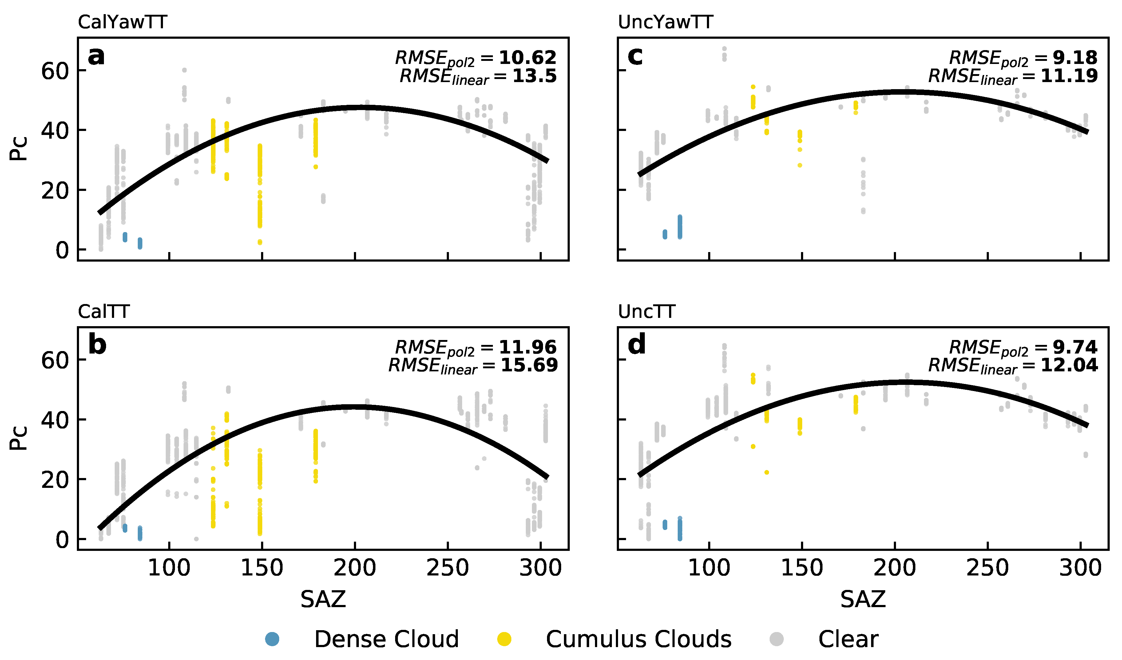
For the analysis of the SEA, only the two optimal settings for geometrically pre-calibrated and on-job calibrated cameras over all land cover classes are displayed (Figure 5). When acquiring data on days with dense cloud cover, the results show bad image alignment for SEA <40. Only one flight with dense cloud cover, which was performed at SEA ~50 shows good alignment with values as high as at clear sky conditions. For cumulus clouds during image acquisition, the alignment seems to be lower but stabilizes for SEA >45. This is especially true when using on-job estimated geometric camera coefficients.
The plots depict a dependency of image alignment on the SEA of a Pearson correlation coefficient higher than 0.5 for pre-calibrated cameras and 0.48 for on-job calibrated cameras, indicating less dependency on illumination when not using geometrically pre-calibrated cameras. It is apparent that especially low SEA (<20) have higher when estimating geometrical camera coefficients during bundle adjustment instead of performing a pre-calibration (Cal). Furthermore, the inclusion of camera orientation metadata in the alignment reduces the variability of for SEA <15, explaining the indicated shift to overall higher values when including camera orientation in Figure 4b.
When weather and land cover effects on correlation are excluded by focusing on the same areas over an entire day with clear sky conditions, we see a similar but more pronounced pattern (Figure 5e–h). A strong correlation between SEA and exists, with lowest Pearson correlation coefficients for UncTT and highest for CalTT. Using the SAA representing the time of the day, we can further note that flights acquired in the evening or late afternoon show higher than data sets acquired at higher SEA for sun rise and morning (see also Figure A1).
3.4. Camera Uncertainty Quantification from Tiepoint Extraction
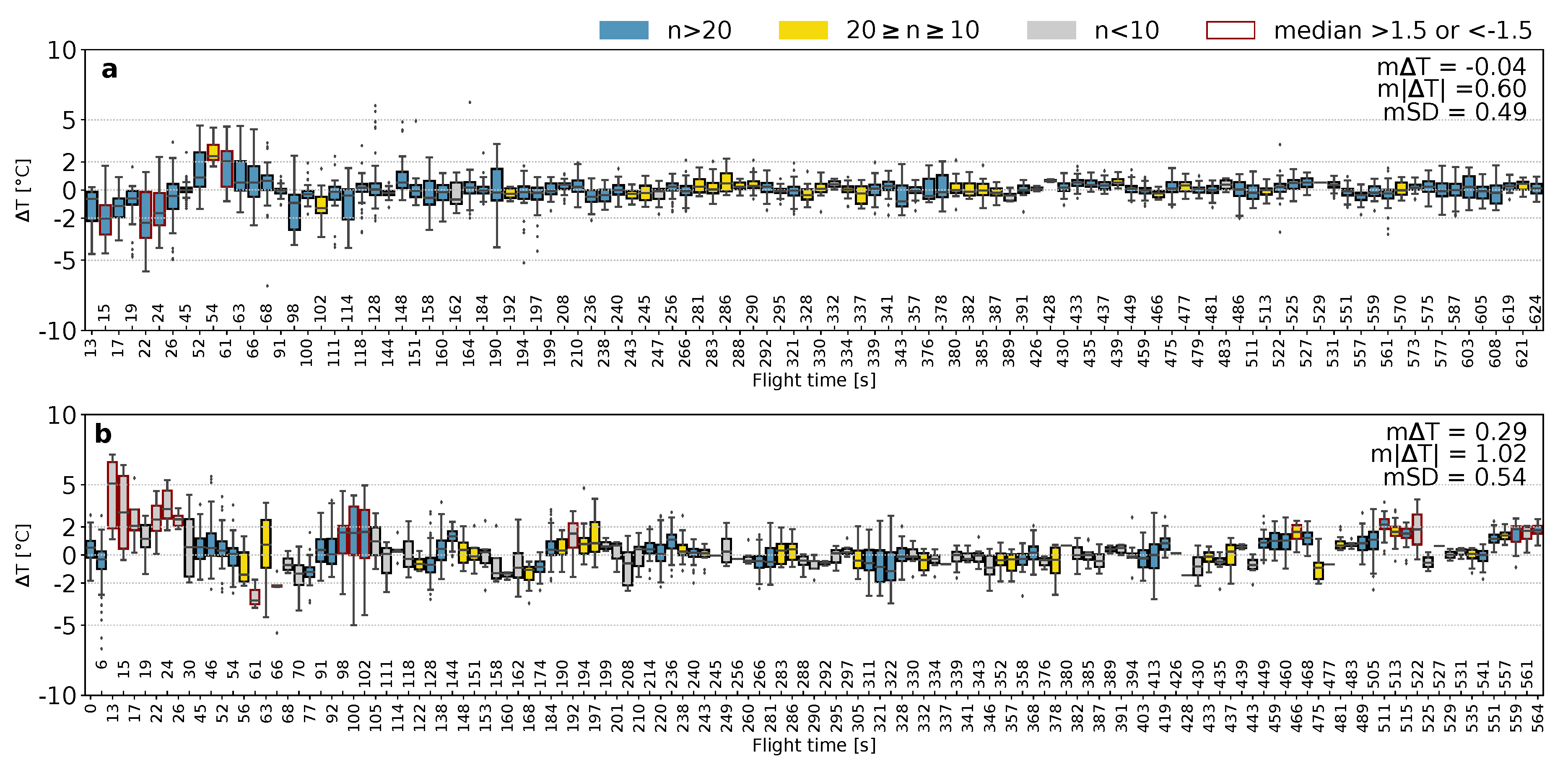
As schematically visualized in Figure 3, the spatially overlapping tiepoints were analyzed to evaluate the sensor stability for each image acquisition. Figure 6 shows the variability of the temperature differences (T) exemplary for a single flight. Every boxplot is composed of temperature differences between identical locations in images that are acquired after a specific time interval to time t and a reference image acquired at this time t. For Figure 6a, identical locations in images acquired a maximum of 4 safter the reference image are compared to the locations in the reference image; for Figure 6b, this time interval is minimum 50 s. The mean difference of the tiepoints to their corresponding counterparts in the reference image is in both cases negative. This indicates a decreasing trend ( if ) of recorded temperature during the image acquisition of the dataset displayed in Figure 6. The trend of decrease is similar for both time differences without any normalization over time.
The arithmetic mean of absolute deviations to each other shows a sensor uncertainty of 0.60 C and a standard deviation of 0.49 C for images acquired with a time difference of maximum 4 s. The absolute difference between tiepoints and their standard deviation for longer time distances (minimum 50 s) is marginally higher. Here, it has to be taken into account that the number of tiepoints that are compared to each other per time is lower in the long-term imagery comparison.
The range or temperature differences per time has higher variation at the beginning of the image acquisition and stabilizes after 110 s in both cases. It is evident that the mean range is far below a T of 2 C, which gives a good impression into the sensor-related uncertainty of the measurements. Moreover, quality changes between flights can be quantified.
The extraction of tiepoints can provide information about the benefit of correcting the image with air temperature data. The statistics of the average of the mean temperature differences, the mean absolute temperature differences, as well as the mean standard deviation of 33 flights performed at site Fendt are summarized in Table 3. The results reveal that the temperature correction does not lead to improvements in any of these statistics. When comparing the means of absolute T between corrected and uncorrected data for each flight, the mean difference is 0.0002 for short time intervals and 0.008 for longer time intervals.
4. Discussion
4.1. Contrast Enhancement
The beneficial impact of contrast enhancement on confirm the results of Ribeiro-Gomes et al. [17]. We are able to add further information regarding the dependence of its effect on land cover classes. It shows highest effect for flights performed over Croplands, where field edges, structures of changing crop types, and gaps between tree or hedge rows exist. These image features result in high texture within the images. Grassland areas are less affected by the filtering. One reason might be the low texture within the image. Ley et al. [37] showed that the standard Wallis filter has a low capacity to increase texture-less features. This observation could also apply to the adapted Wallis filter. Brad [24] note the preservation of texture-less areas as uniform after applying their adapted filter, which confirms this hypothesis. Some authors propose to first reduce image noise and then apply the Wallis filter for feature detection [37,38]. Concerning the Forest land cover class, overall image alignment is rather unsuitable. The low effect of contrast enhancement is indicative of other factors causing problems in feature matching rather than contrast itself.
We found no outstanding differences in the parameters of the filter. Increasing the parameters of a Wallis filter showed a saturation of the amount of detected and matched features [38]. Assuming a similar behavior for the adapted filter used in our analysis, the chosen parameter range could be too high to cause significant changes for feature detection and matching. A further analysis of the acquisition time (sun azimuth angle) could perhaps lead to a more differentiated image when searching for optimal parameters of the filter applied here.
4.2. Camera Calibration
Maes et al. [15] show a very small effect on camera calibration when no GPS data is considered for image alignment. Our analysis shows that the camera calibration has no merit for image alignment, as it decreases the number of points per alignable image and increases alignment instability. Questions arise on the stability of estimated camera coefficients when operating the camera at different temperatures than the acquired images for geometric camera estimation, as lens elements could slightly move or expand. Furthermore, vibrations caused by the vehicle can lead to different coefficients. Considering this, estimated camera coefficients might differ from real camera coefficients during each image acquisition, decreasing the capacity to correct for distortions and thus match features.
Nevertheless, Luhmann et al. [26] states the importance of geometric camera calibration for mosaic creation. This can also be performed during the bundle adjustment. Harwin et al. [27] showed that this approach leads to satisfying results combined with low workload during data acquisition, whereas camera calibration using the checkerboard pre-calibration at distances lower than the later flight altitudes performs worse in point cloud accuracy. The results of our analysis with TIR imagery are consistent with their findings. Further analysis of geometric camera pre-calibration on feature matching and point cloud accuracy for thermal imagery at distances to the calibration pattern corresponding to flight altitudes should be performed.
4.3. Pre-Selection Methods
For Grassland and Cropland, both pre-selection methods lead to improvements in . Besides speeding up the process of image alignment, both applications filter the input images according to their position (reference pre-selection) or potential overlapping areas (generic pre-selection). In doing so, they reduce the probability of incorrect feature mapping by decreasing the number of possible match areas. When both settings are used, the number of potentially adjacent images for feature matching is reduced even more. The reference criterion first selects a certain number of neighboring images according to the source coordinates. Then the generic preselection is additionally applied, which further reduces the number of possible matching images (personal communication Agisoft team, 4 March 2020). The filter of the images might reduce the number of wrong matches that hamper the overall alignment.
The slight improvement when also using reference pre-selection show the importance of including the image location in the alignment process, as longitude and latitude are considered in the feature matching and search process. These results confirm the beneficial effect of GPS inclusion found by Maes et al. [15]. Since the generic pre-selection and reference pre-selection filter possible locations very well even without the yaw angle, the inclusion of the vehicle orientation in the alignment process shows only minor benefit. The low amount of changes in possible overlapping areas or neighboring images has marginal effect on the amount of detected and matched features. There might be additional effects when including Pitch and Roll angle instead of assuming 0 for both. Therefore, a GPS and compass module positioned on the camera would be necessary for image acquisition with a gimbal to insert high-precision viewing angle deviations due to gimbal uncertainty.
4.4. SEA and Weather
For times of low illumination, such as low SEA or high cloud coverage, values indicate an inferior image alignment. The increasing contrast between canopy and ground with increasing SEA is reported by several authors [39,40]. The comparison of mean standard deviation within images of every data set with SEA confirms the same trend in our case (see Figure A2). The basic SfM algorithm used in Agisoft is similar to the Scale-Invariant Feature Transform (SIFT) algorithm [41]. As the main limitation of SIFT is its dependency of texture and image contrast [42], the observed pattern can be related to problems in contrast of imagery. Due to the acquisition over same areas in one day, we are also able to prove that the effect of decrease in image alignment is less in afternoon hours. This corresponds to a delayed cooling of the soil surface after the solar zenith angle [43], whereby the variation of the surface temperatures, and thus a higher image contrast than in the morning hours is maintained.
The deterioration of image alignment with increasing cloud cover is very pronounced for SEA <20 and decreases with increasing SEA. One data set, acquired on a very cloudy day (9 July 2019) at high SEA, has the same values as other flights of the same land cover class with comparable SEA. In contrast, other data sets acquired on very cloudy days at low SEA have the overall lowest . This indicates that the differential heating of surface materials is delayed during the morning due to the dense cloud cover. Having differential heating of the imaged objects resulted in sufficient image texture for image alignment, even a dense cloud cover does not hinder image alignment. Nevertheless, further imagery would be needed to confirm this hypothesis.
When acquiring imagery at changing illumination conditions during the image acquisition (cumulus clouds), we notice no difference to data sets acquired over the same land cover and similar SEA with stable illumination conditions. The signal of the camera can be hampered in two ways with changing weather conditions. First of all, changes in the surrounding temperature of the sensor can induce temperature changes in the FPA faster than the operation of the shutter [13]. Second of all, the signal is hampered by reflected sky radiation [44]. Variation of both noise factors cause changes in the overall grayscale level of the acquired TIR image. The robustness of the image alignment can therefore be based either on a very high signal-to-noise ratio of the camera or the robustness of SIFT against changes in the grayscale level [42].
On-job geometric camera coefficient estimation delivers higher values with higher reliability. The high dependency on SEA when using camera distortion coefficients of the pre-calibrated camera can be related to the different surrounding temperature of the camera. The morning and evening temperatures deviate most from the midday temperatures at which the images for the coefficient estimation were acquired. With increasing surrounding temperature corresponding to high SEA, the temperature converges to the sensor temperature at image acquisition for the geometrical pre-calibration pattern.
4.5. Land Cover Effect
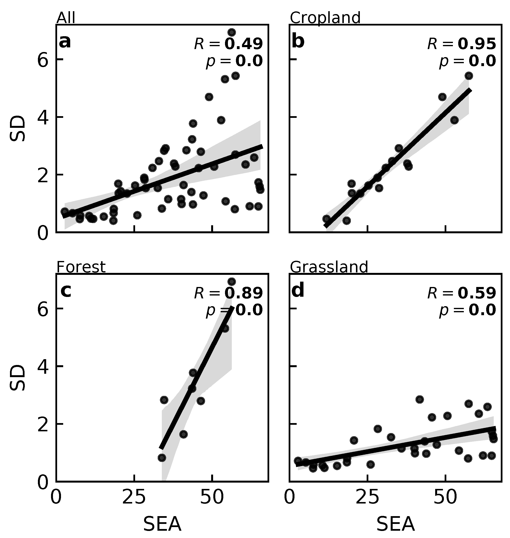
Generally, we observe a strong dependency of image alignment quality on land cover, which has to be taken into account for field campaign planning, e.g., via choosing higher overlapping rates. Regarding the ranking of land cover types, it was unexpected that Cropland has less than Grassland. Homogeneous areas such as grassland are assumed to be more difficult to align [15]. Additionally, contrast was found to have significant effect on feature matching in former studies [15,42]. In our results we are able to relate the positive impact of increasing SEA to a rise in contrast. Nevertheless, when comparing mean SD within images (see Table 2) as an indicator of contrast, we note that Grassland has the lowest contrast values among all land cover types, while at the same time it has the highest values. The reverse is true for Forests. Therefore, we conclude that contrast within images is not the only factor of image characteristics that influences image alignment. This is further underlined by the low effect of contrast enhancement on image alignment of the Forest land cover class.
With our analysis we are able to statistically confirm the expectations of Maes et al. [15], namely, that forests cause more problems in image alignment. They state that the complexity in canopy structure is a problematic feature for image alignment. When considering canopy complexity as indicated by canopy height we can confirm the trend with our data with Grassland having lowest complexity and canopy height, followed by Cropland and Forest. With higher canopy height the exposure to wind increases, leading to changes in canopy structure. This could cause the problems in image alignment.
Furthermore, the variation of a feature shape is much greater for complex canopy structures compared to flat surfaces. This is related to the different heights of the objects imaged, which range from the ground surface to understory vegetation and the tree canopy. The complexity in the structure creates a higher variety in sun–surface–sensor geometries, which leads to stronger distortions in observed features. These distortions are further enhanced by TIR directional effects [45]. The directional effects are driven by leaf angular distribution and the temperature difference between shaded and non-shaded areas, among other aspects [46]. Different viewing angles related to the sensor geometry can cause a complete inversion of relative brightness relations among pixels and thus change the appearance of identical features. Lowe [42] reports the SIFT algorithm as robust against linear and nonlinear changes of image brightness. Nevertheless, he points out that rotations of more than 30 combined with changes in illumination will impair feature matching.
Texture of imagery differs per land cover type [47]. Therefore, feature characteristics such as size and shape also differ. SIFT offers the opportunity to match features invariant to their scale. Nevertheless, the detection of features is dependent on local maxima of a Gaussian kernel with specific size of sigma. The bigger the scales of this kernel, the higher the probability is that local maxima caused by keypoints of bigger size overlap. Therefore, threshold of local maxima intensities are set [42]. Depending on the thresholds set and the size of the kernel for the feature matching algorithm in Agisoft, the features of a low resolved forest imagery can be too big to be captured by the algorithm implemented in Agisoft. Further analysis on typical feature size per land cover type could assess this hypothesis.
Dandois et al. [48] and Seifert et al. [49] deal with challenges of accurate image alignment for RGB imagery over forests. They report high dependency of point cloud density on forward overlap ( 90%) and ground sampling distance when using SfM for RGB cameras for forest structure assessment. As SfM depends highly on different viewing angles of one detected feature, forward overlap assures this requirement. The number of valid matches is additionally improved by a high variety of the viewing angle. Therefore, flying at lower altitudes increases intrinsic distortions of images, which leads to a higher variation in viewing angles combined with a higher detail of the acquired image, leading to higher numbers of tiepoints. Those findings of the influence in RGB can also apply for TIR cameras and should be considered for image acquisitions over forested areas, although it reduces the area which can be covered significantly.
Dandois et al. [48] further reveal the importance of high resolution of the image for point cloud density when acquiring data of forests for RGB imagery (10 MP). For TIR cameras with MP of less than 1 MP, this effect is can be decisive. Lower flight altitudes over forest areas or higher resolved TIR cameras by maintaining a high forward overlap of 80–90% could lead to better results.
4.6. Camera Uncertainty Quantification
The tiepoints extraction allows a quantification of camera noise of ~1.5 C. The estimated uncertainty of the camera measurements is lower than those estimated by Ribeiro-Gomes et al. [17] for the same camera with higher spatial resolution. They reached similar accuracy with additional calibration of the sensor. The positive results of our camera without additional calibration possibly originate from the additional external housing and heated shutter platform. Furthermore, we assessed the stability of the sensor’s own measurements instead of comparing them to target temperatures.
The benefit of this approach is the assessment of camera accuracy based on the acquired imagery itself. Accuracy is affected by environmental conditions such as clouds or wind [13]. Those conditions vary for every image acquisition. An assessment of measurement accuracy is therefore necessary for each single flight. Our approach allows the assessment of uncertainty within each data set individually without further ground truth measurements or reference panels.
The temperature correction of Maes et al. [15] has no significant effect on camera uncertainty considering the results of the tiepoint extraction. This result can be related to the coarse temporal resolution of 1 min of the meteorological background data compared to the less than 5 s time difference between the single image acquisitions. Furthermore, air temperature records at 2 m altitude cause anomalies estimated via a spline function of maximal 0.68 C. Even the maximal correction factor applied to the imagery accounts for only one-third of the mean absolute deviation of the camera.
This observation leads to the assumption that the main error source of uncertainty is not based in the changes of air temperatures at ground level causing rapid changes in ground surface temperature [15], but rather by thermal drift associated with changes of the temperature or wind surrounding the sensor. This explanation is supported by the overall negative trend of all acquired flights, reflecting the cooler temperatures with increasing flight altitude of the camera.
The increased uncertainty in image data at the start of the image acquisition corresponds to the findings of Kelly et al. [13]. They propose additional flight lines at the beginning of the image acquisition. This requirement is further confirmed by this study and the overall negative trend in image errors in all flights, revealing the cooling of the sensor when being moved to lower air temperatures with increasing flight height. Adding further flight lines reduces the area that can be covered. Our uncertainty assessment allows for a definition of a time span of imagery impacted by sensor stabilization. It is possible to exclude this data or treat those areas carefully for radiometric use. For other image acquisitions and environmental conditions, this stabilization time might vary due to lower temperature differences between ground temperature and temperature at flight altitude. Therefore, this approach offers the opportunity to identify noisy imagery with rapidly changing environmental conditions for each flight. Further analysis on the dependency of flight stabilization on time of the day, wind, or air pressure conditions could lead to more elaborated recommendations for stable image acquisition.
Mesas-Carrascosa et al. [14] and Jensen et al. [50] try to decrease the effect of thermal drift by modeling it using the change of temperature per time. Nevertheless, they include all tiepoints without considering their temporal intervals in their modelling. Referring to our results, errors along time behave differently when considering different time intervals of uncertainty extraction. In the displayed case, long-term differences account for a mean T of 0.029 C per second, whereas short-term differences account for a mean T of −0.04 C per second. Using the short-term tiepoints to correct for thermal drift would lead to an over correction of the images and to higher deviations in long-term tiepoint observations. This needs to be considered when modeling the thermal drift based on extracted tiepoints. An analysis of the perfect time interval between tiepoints is necessary for an optimal correction of the imagery.
Considering the short time interval as sensor noise rather than systematic temperature drift, we can also detect images that have higher deviations from other images and exclude them from the creation of orthomosaic for the sake of radiometric accuracy.
When applying the approach presented here, directional effects which are not negligible within TIR [39,45] must be taken into account. Modeling results of Duffour et al. [45] show deviations of up to 15 C depending on canopy structure, meteorological forcing imposed at the surface, the surface water stress level, as well as the azimuth and zenith viewing angle. Lagouarde et al. [39] measured lower differences to the nadir look angle considering varying solar azimuth angles (0.5–4 C). These results point to the need for further research to separate bidirectional effects from uncertainty.
So far, we assume a minimization of the spatial heterogeneity of the sensor due to the application of the external shutter. Nevertheless, taking the position within the sensor geometry of each tiepoint into account could give meaningful insights on heterogeneities along the FPA.
5. Conclusions
Image alignment and radiometric accuracy of thermal imagery acquired with UAS and low-cost TIR cameras face several challenges. We analyzed a big data set comprising 56 single flight acquisitions at different times of the day with associated changing SEA, over three different land cover types and at different weather situations. We included best practices of former research papers in our image acquisition and preprocessing chain and are now able to give the following suggestions for TIR data image acquisition and preprocessing based on a valid statistical analysis.
- For the creation of orthomosaics, high SEA are favorable due to their higher contrast. This is especially important for land cover types and weather conditions that are problematic in image alignment such as forest or overcast sky conditions.
- When analyzing temperature differences throughout the day, the probability of aligned imagery is higher in the evening than in the morning for the same SEA.
- Results concerning land cover types reveal major problems of image alignment over forested areas. The analysis of our data set proposes an image acquisition on clear sky conditions at maximal SEA. Related research on RGB imagery further propose higher resolution or flying at lower altitude with lower velocity. A high forward and side overlap yields better results.
- We propose a stabilization time of a minimum of 60 sto allow the sensor temperature to adapt to air temperatures at flight altitude or adding additional flight lines [13].
- Contrast enhancement of the imagery significantly improves the number of detected features.
- The inclusion of geometric camera calibration estimates using a regular image pattern hampers image alignment and should be avoided.
- We recommend the application of both pre-selection methods supplied in Agisoft Metashape for aligning the imagery. In case no GPS information for each image is available, we propose to only match features within overlapping areas as implemented in the Generic Pre-selection option of Agisoft Metashape.
- We further are able to show that the inclusion of UAS orientation background data is not necessary for SEA higher than 30 and 40 for sunny and cloudy days, respectively. For SEA <15, the inclusion of UAS orientation information increases the probability of a high number of points in the point cloud.
- The proposed method of temperature correction after Maes et al. [15] did not lead to a reduction in camera uncertainty in long and short-term noise.
- We strongly advocate for the uncertainty quantification of the camera and recommend the approach presented here. This approach also has the potential to identify and remove single images with high measurement uncertainty.
To establish a rule of thumb on stabilization time at flight altitude, further research is needed on the impact of temperature difference between temperature at ground and flight altitude, air pressure, or wind on the length of noisy image at the start of the flight. When correcting for temperature drift, the time span between analyzed tiepoints needs to be taken into account. Several authors acquire thermal data simultaneously with RGB or multispectral data, using this additional information for image alignment [9,15]. This has been shown to further improve image alignment [15] and can overcome limitations of image alignment over forests. Nevertheless, systematic research concerning best practices for thermal image alignment over forest canopy is necessary.
Author Contributions
Conceptualization, V.D., T.G., and M.F.; methodology, V.D. and T.G.; formal analysis, V.D.; resources, T.G. and V.D.; data curation, T.G. and V.D.; writing—original draft preparation, V.D.; writing—review and editing, all authors; supervision, M.F. and B.K.; project administration, B.K. and M.F.; funding acquisition, B.K. and M.F. All authors have read and agreed to the published version of the manuscript.
Funding
This research was funded by Deutsche Forschungsgemeinschaft (DFG) project no. 357874777 of the research unit for 2694 “Cosmic Sense”. The Terrestrial Environmental Observatory (TERENO) Pre-Alpine infrastructure is funded by the Helmholtz Association and the Federal Ministry of Education and Research.
Acknowledgments
We would like to thank the ATB Marquardt for use of their research station area as a site to perform our UAS flights. We further express our gratitude to Paterzell Airfield Control for their cooperation and permission to use their airspace for UAS-based data acquisition. In this context, we also want to thank Matthias Zeeman (KIT) for the coordination of UAS teams and schedules at the Fendt testsite. We thank Arlena Brosinski (Uni Potsdam) for support the flight campaign in Treuenbrietzen. We thank all landowners granting permission to access their property. The effort for data acquisition and imagery preprocessing was only possible thanks to the help of our student assistance Florencia Arias.
Conflicts of Interest
The authors declare no conflicts of interest. The funders had no role in the design of the study; in the collection, analyses, or interpretation of data; in the writing of the manuscript; or in the decision to publish the results.
Abbreviations
The following abbreviations are used in this manuscript:
| CE | contrast enhancement |
| UAS | Unmanned aerial system |
| SfM | Structure for Motion |
| NUC | Nonuniformity correction |
| FPA | Focal plane array |
| TIR | Thermal Infrared |
| SIFT | Scale-Invariant Feature Transform |
| IQR | Interquantile Range |
| IR | Infrared |
| RGB | Red Green Blue |
| SAZ | Sun azimuth angle |
| SEA | Sun elevation angle |
Appendix A
Figure A1.
Stability of (c) UncYaTT in alignment of data sets acquired with Cumulus clouds covering the sky over Grassland areas in comparison to (a) CalYawTT, (b) CalTT and (d) UncTT and better fit of polynomial regression of PC along Sun azimuth angle.
Figure A1.
Stability of (c) UncYaTT in alignment of data sets acquired with Cumulus clouds covering the sky over Grassland areas in comparison to (a) CalYawTT, (b) CalTT and (d) UncTT and better fit of polynomial regression of PC along Sun azimuth angle.


Table A1.
Camera distortion coefficients.
| f | cx | cy | B1 | B2 | k1 | k2 | k3 | k4 | P1 | P2 | P3 | P4 |
|---|---|---|---|---|---|---|---|---|---|---|---|---|
| 124.64 | 17.44 | 16.99 | 0.27 | 0.034 | −0.033 | −0.0014 | 0.005 | −0.001 | −1.092 × 10−06 | −1.001 × 10−06 | −20.51 | 89 |
Figure A2.
Correlation of sun elevation angle and standard deviation per land cover type. (a) All; (b) Cropland; (c) Forest; (d) Grassland.
Figure A2.
Correlation of sun elevation angle and standard deviation per land cover type. (a) All; (b) Cropland; (c) Forest; (d) Grassland.

Figure A3.
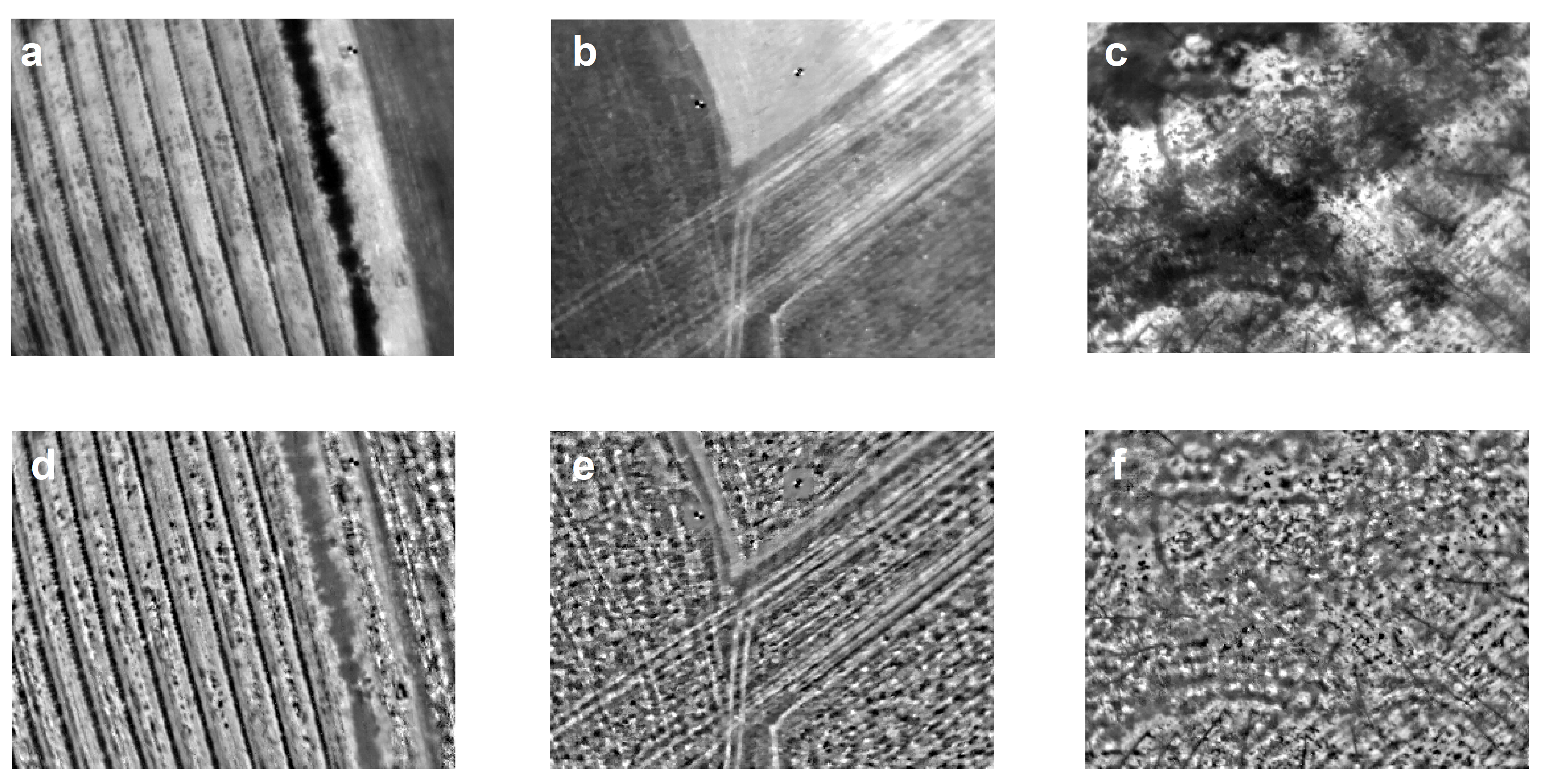
Example images for each land cover class. (a) Cropland, acquisition start: 2019-07-09T12:46:13.6Z, (b) Grassland, acquisition start: 2019-06-05T12:22:00.2Z, (c) Forest, acquisition start: 2019-07-11T12:51:34.6Z, (d) contrast enhanced cropland, (e) contrast enhanced grassland, (f) contrast enhanced forest. contrast enhancement settings: A = 150, B = 25.
Figure A3.
Example images for each land cover class. (a) Cropland, acquisition start: 2019-07-09T12:46:13.6Z, (b) Grassland, acquisition start: 2019-06-05T12:22:00.2Z, (c) Forest, acquisition start: 2019-07-11T12:51:34.6Z, (d) contrast enhanced cropland, (e) contrast enhanced grassland, (f) contrast enhanced forest. contrast enhancement settings: A = 150, B = 25.

References
- Pachauri, R.K.; Allen, M.R.; Barros, V.R.; Broome, J.; Cramer, W.; Christ, R.; Church, J.A.; Clarke, L.; Dahe, Q.; Dasgupta, P.; et al. Climate Change 2014: Synthesis Report. Contribution of Working Groups I, II and III to the Fifth Assessment Report of the Intergovernmental Panel on Climate Change; IPCC: Geneva, Switzerland, 2014. [Google Scholar]
- Hu, T.; Renzullo, L.J.; van Dijk, A.I.; He, J.; Tian, S.; Xu, Z.; Zhou, J.; Liu, T.; Liu, Q. Monitoring agricultural drought in Australia using MTSAT-2 land surface temperature retrievals. Remote Sens. Environ. 2020, 236, 111419. [Google Scholar] [CrossRef]
- Langer, M.; Westermann, S.; Boike, J. Spatial and temporal variations of summer surface temperatures of wet polygonal tundra in Siberia-implications for MODIS LST based permafrost monitoring. Remote Sens. Environ. 2010, 114, 2059–2069. [Google Scholar] [CrossRef]
- Bai, L.; Long, D.; Yan, L. Estimation of surface soil moisture with downscaled land surface temperatures using a data fusion approach for heterogeneous agricultural land. Water Resour. Res. 2019, 55, 1105–1128. [Google Scholar] [CrossRef]
- Kumar, K.S.; Bhaskar, P.U.; Padmakumari, K. Estimation of land surface temperature to study urban heat island effect using LANDSAT ETM+ image. Int. J. Eng. Sci. Technol. 2012, 4, 771–778. [Google Scholar]
- Masoudi, M.; Tan, P.Y. Multi-year comparison of the effects of spatial pattern of urban green spaces on urban land surface temperature. Landsc. Urban Plan. 2019, 184, 44–58. [Google Scholar] [CrossRef]
- Egea, G.; Verhoef, A.; Vidale, P.L. Towards an improved and more flexible representation of water stress in coupled photosynthesis–stomatal conductance models. Agric. Forest Meteorol. 2011, 151, 1370–1384. [Google Scholar] [CrossRef]
- Berni, J.; Zarco-Tejada, P.; Sepulcre-Cantó, G.; Fereres, E.; Villalobos, F. Mapping canopy conductance and CWSI in olive orchards using high resolution thermal remote sensing imagery. Remote Sens. Environ. 2009, 113, 2380–2388. [Google Scholar] [CrossRef]
- Brenner, C.; Thiem, C.E.; Wizemann, H.D.; Bernhardt, M.; Schulz, K. Estimating spatially distributed turbulent heat fluxes from high-resolution thermal imagery acquired with a UAV system. Int. J. Remote Sens. 2017, 38, 3003–3026. [Google Scholar] [CrossRef] [Green Version]
- Nieto, H.; Kustas, W.P.; Torres-Rúa, A.; Alfieri, J.G.; Gao, F.; Anderson, M.C.; White, W.A.; Song, L.; del Mar Alsina, M.; Prueger, J.H.; et al. Evaluation of TSEB turbulent fluxes using different methods for the retrieval of soil and canopy component temperatures from UAV thermal and multispectral imagery. Irrig. Sci. 2019, 37, 389–406. [Google Scholar] [CrossRef] [Green Version]
- Pádua, L.; Vanko, J.; Hruška, J.; Adão, T.; Sousa, J.J.; Peres, E.; Morais, R. UAS, sensors, and data processing in agroforestry: A review towards practical applications. Int. J. Remote Sens. 2017, 38, 2349–2391. [Google Scholar] [CrossRef]
- Olbrycht, R.; Więcek, B. New approach to thermal drift correction in microbolometer thermal cameras. Quant. InfraRed Thermogr. J. 2015, 12, 184–195. [Google Scholar] [CrossRef]
- Kelly, J.; Kljun, N.; Olsson, P.O.; Mihai, L.; Liljeblad, B.; Weslien, P.; Klemedtsson, L.; Eklundh, L. Challenges and best practices for deriving temperature data from an uncalibrated UAV thermal infrared camera. Remote Sens. 2019, 11, 567. [Google Scholar] [CrossRef] [Green Version]
- Mesas-Carrascosa, F.J.; Pérez-Porras, F.; Meroño de Larriva, J.E.; Mena Frau, C.; Agüera-Vega, F.; Carvajal-Ramírez, F.; Martínez-Carricondo, P.; García-Ferrer, A. Drift correction of lightweight microbolometer thermal sensors on-board unmanned aerial vehicles. Remote Sens. 2018, 10, 615. [Google Scholar] [CrossRef] [Green Version]
- Maes, W.H.; Huete, A.R.; Steppe, K. Optimizing the processing of UAV-based thermal imagery. Remote Sens. 2017, 9, 476. [Google Scholar] [CrossRef] [Green Version]
- Berni, J.A.; Zarco-Tejada, P.J.; Suárez, L.; Fereres, E. Thermal and narrowband multispectral remote sensing for vegetation monitoring from an unmanned aerial vehicle. IEEE Trans. Geosci. Remote Sens. 2009, 47, 722–738. [Google Scholar] [CrossRef] [Green Version]
- Ribeiro-Gomes, K.; Hernández-López, D.; Ortega, J.F.; Ballesteros, R.; Poblete, T.; Moreno, M.A. Uncooled thermal camera calibration and optimization of the photogrammetry process for UAV applications in agriculture. Sensors 2017, 17, 2173. [Google Scholar] [CrossRef]
- Torres-Rua, A. Vicarious calibration of sUAS microbolometer temperature imagery for estimation of radiometric land surface temperature. Sensors 2017, 17, 1499. [Google Scholar] [CrossRef] [Green Version]
- Schönberger, J.L.; Frahm, J. Structure-from-Motion Revisited. In Proceedings of the 2016 IEEE Conference on Computer Vision and Pattern Recognition (CVPR), Las Vegas, NV, USA, 26 June–1 July 2016; pp. 4104–4113. [Google Scholar] [CrossRef]
- Canon Deutschland GmbH. Unsere Auswahl an EOS DSLR-Kameras. Available online: https://www.canon.de/cameras/dslr-cameras-range (accessed on 30 March 2020).
- Hoffmann, H.; Nieto, H.; Jensen, R.; Guzinski, R.; Zarco-Tejada, P.; Friborg, T. Estimating evaporation with thermal UAV data and two-source energy balance models. Hydrol. Earth Syst. Sci 2016, 20, 697–713. [Google Scholar] [CrossRef] [Green Version]
- Pech, K.; Stelling, N.; Karrasch, P.; Maas, H. Generation of multitemporal thermal orthophotos from UAV data. Int. Arch. Photogramm. Remote Sens. Spat. Inf. Sci. 2013, 1, 305–310. [Google Scholar] [CrossRef] [Green Version]
- Wallis, R.H. An approach for the space variant restoration and enhancement of images. In Proceedings of the Symposium on Current Mathematical Problems in Image Science, Montery, CA, USA, 10–12 November 1976. [Google Scholar]
- Brad, R. Satellite Image Enhancement by Controlled Statistical Differentiation. In Innovations and Advanced Techniques in Systems, Computing Sciences and Software Engineering; Elleithy, K., Ed.; Springer: Dordrecht, The Netherlands, 2008; pp. 32–36. [Google Scholar]
- Brenner, C.; Zeeman, M.; Bernhardt, M.; Schulz, K. Estimation of evapotranspiration of temperate grassland based on high-resolution thermal and visible range imagery from unmanned aerial systems. Int. J. Remote Sens. 2018, 39, 5141–5174. [Google Scholar] [CrossRef] [Green Version]
- Luhmann, T.; Piechel, J.; Roelfs, T. Geometric calibration of thermographic cameras. In Thermal Infrared Remote Sensing; Springer: Dordrecht, The Netherlands, 2013; pp. 27–42. [Google Scholar] [CrossRef] [Green Version]
- Harwin, S.; Lucieer, A.; Osborn, J. The impact of the calibration method on the accuracy of point clouds derived using unmanned aerial vehicle multi-view stereopsis. Remote Sens. 2015, 7, 11933–11953. [Google Scholar] [CrossRef] [Green Version]
- Kiese, R.; Fersch, B.; Bassler, C.; Brosy, C.; Butterbach-Bahlc, K.; Chwala, C.; Dannenmann, M.; Fu, J.; Gasche, R.; Grote, R.; et al. The TERENO Pre-Alpine Observatory: Integrating Meteorological, Hydrological, and Biogeochemical Measurements and Modeling. Vadose Zone J. 2018, 17, 180060. [Google Scholar] [CrossRef]
- Sands, P.J. Prediction of vignetting. J. Opt. Soc. Am. 1973, 63, 803–805. [Google Scholar] [CrossRef]
- Ciocia, C.; Marinetti, S. In-situ emissivity measurement of construction materials. In Proceedings of the 11th International Conference on Quantitative InfraRed Thermography, Naples, Italy, 11–14 June 2012. [Google Scholar]
- Agisoft LLC. Agisoft Metashape User Manual; Professional edition; Version 1.5; AgiSoft LLC: Petersburg, Russia, 2019. [Google Scholar]
- DWD Climate Data Center (CDC). Auswahl von 81 über Deutschland verteilte Klimastationen, im Traditionellen KL-Format, Version Recent. Available online: https://opendata.dwd.de/climate_environment/CDC/observations_germany/climate/subdaily/standard_format/ (accessed on 7 May 2020).
- Turner, D.; Lucieer, A.; Wallace, L. Direct georeferencing of ultrahigh-resolution UAV imagery. IEEE Trans. Geosci. Remote Sens. 2013, 52, 2738–2745. [Google Scholar] [CrossRef]
- Fraser, B.T.; Congalton, R.G. Issues in Unmanned Aerial Systems (UAS) data collection of complex forest environments. Remote Sens. 2018, 10, 908. [Google Scholar] [CrossRef] [Green Version]
- Earth System Research Laboratory, NOAA. NOAA Solar Calculator. Available online: http://www.esrl.noaa.gov/gmd/grad/solcalc (accessed on 15 January 2020).
- Wierzbicki, D.; Kedzierski, M.; Fryskowska, A. Assesment of the influence of uav image quality on the orthophoto production. Int. Arch. Photogramm. Remote Sens. Spat. Inf. Sci. 2015, 40, 1. [Google Scholar] [CrossRef] [Green Version]
- Ley, A.; Hänsch, R.; Hellwich, O. Reconstructing white walls: Multi-view, multi-shot 3d reconstruction of textureless surfaces. ISPRS Ann. Photogramm. Remote Sens. Spat. Inf. Sci. 2016, 3, 91–98. [Google Scholar] [CrossRef]
- Ballabeni, A.; Apollonio, F.I.; Gaiani, M.; Remondino, F. Advances in Image Pre-processing to Improve Automated 3D Reconstruction. Int. Arch. Photogramm. Remote Sens. Spat. Inf. Sci. 2015, 315–323. [Google Scholar] [CrossRef] [Green Version]
- Lagouarde, J.; Kerr, Y.; Brunet, Y. An experimental study of angular effects on surface temperature for various plant canopies and bare soils. Agric. Forest Meteorol. 1995, 77, 167–190. [Google Scholar] [CrossRef]
- Bellvert, J.; Zarco-Tejada, P.J.; Girona, J.; Fereres, E. Mapping crop water stress index in a ‘Pinot-noir’vineyard: Comparing ground measurements with thermal remote sensing imagery from an unmanned aerial vehicle. Precis. Agric. 2014, 15, 361–376. [Google Scholar] [CrossRef]
- Dandois, J.P.; Ellis, E.C. High spatial resolution three-dimensional mapping of vegetation spectral dynamics using computer vision. Remote Sens. Environ. 2013, 136, 259–276. [Google Scholar] [CrossRef] [Green Version]
- Lowe, D.G. Distinctive image features from scale-invariant keypoints. Int. J. Comput. Vis. 2004, 60, 91–110. [Google Scholar] [CrossRef]
- Deardorff, J.W. Efficient prediction of ground surface temperature and moisture, with inclusion of a layer of vegetation. J. Geophys. Res. Oceans 1978, 83, 1889–1903. [Google Scholar] [CrossRef] [Green Version]
- Highnam, R.; Brady, M. Model-based image enhancement of far infrared images. IEEE Trans. Pattern Anal. Mach. Intell. 1997, 19, 410–415. [Google Scholar] [CrossRef]
- Duffour, C.; Lagouarde, J.P.; Roujean, J.L. A two parameter model to simulate thermal infrared directional effects for remote sensing applications. Remote Sens. Environ. 2016, 186, 250–261. [Google Scholar] [CrossRef]
- Duffour, C.; Lagouarde, J.P.; Olioso, A.; Demarty, J.; Roujean, J.L. Driving factors of the directional variability of thermal infrared signal in temperate regions. Remote Sens. Environ. 2016, 177, 248–264. [Google Scholar] [CrossRef]
- Lark, R. Geostatistical description of texture on an aerial photograph for discriminating classes of land cover. Int. J. Remote Sens. 1996, 17, 2115–2133. [Google Scholar] [CrossRef]
- Dandois, J.P.; Olano, M.; Ellis, E.C. Optimal altitude, overlap, and weather conditions for computer vision UAV estimates of forest structure. Remote Sens. 2015, 7, 13895–13920. [Google Scholar] [CrossRef] [Green Version]
- Seifert, E.; Seifert, S.; Vogt, H.; Drew, D.; Van Aardt, J.; Kunneke, A.; Seifert, T. Influence of drone altitude, image overlap, and optical sensor resolution on multi-view reconstruction of forest images. Remote Sens. 2019, 11, 1252. [Google Scholar] [CrossRef] [Green Version]
- Jensen, A.M.; McKee, M.; Chen, Y. Procedures for processing thermal images using low-cost microbolometer cameras for small unmanned aerial systems. In Proceedings of the 2014 IEEE Geoscience and Remote Sensing Symposium, Quebec City, QC, Canada, 13–18 July 2014; pp. 2629–2632. [Google Scholar] [CrossRef]
Figure 1.
Areas overflown by site, land cover, date, and time. (a) Schedule, site, and land cover of different data acquisitions. (b) Flights and assigned land cover type for Fendt, (c) Marquardt, (d) and for Treuenbrietzen. (Basemap: Satellite Google, Imagery 2020, GeoBasis-DE/BKG, GeoContent, Maxar Technologies).

Figure 2.
Image acquisition equipment. (a) Flir Tau 2 336 with external heated shutter system. (b) MK Okto XL 6S12.
Figure 2.
Image acquisition equipment. (a) Flir Tau 2 336 with external heated shutter system. (b) MK Okto XL 6S12.

Figure 3.
Scheme of tiepoint extraction and calculation of uncertainty measures. number of the image.
Figure 3.
Scheme of tiepoint extraction and calculation of uncertainty measures. number of the image.

Figure 4.
(a) per contrast enhancement settings and land cover. The color groups stand for parameter A, their different brightness levels mark parameter B (b) per combination of IMU data inclusion, geometric camera calibration, and pre-selection options (see abbreviations in Table 1). Gray shades highlight calibrated and on-job geometric camera calibration

Figure 5.
Pc per sun elevation angle (SEA) and weather conditions for (a) CalYawTT, (b) CalTT, (c) UncYawTT, and (d) UncTT and PC per SEA at clear sky conditions over same areas during one day for (e) CalYawTT, (f) CalTT, (g) UncYawTT, and (h) UncTT.
Figure 5.
Pc per sun elevation angle (SEA) and weather conditions for (a) CalYawTT, (b) CalTT, (c) UncYawTT, and (d) UncTT and PC per SEA at clear sky conditions over same areas during one day for (e) CalYawTT, (f) CalTT, (g) UncYawTT, and (h) UncTT.

Figure 6.
Temperature differences at time t of features in images acquired within (a) the next 4 s(b) minimum 50 sto paired features in image acquired at time t. n is the number of tiepoints. Please note the non-continuous and non-identical time scaling.
Figure 6.
Temperature differences at time t of features in images acquired within (a) the next 4 s(b) minimum 50 sto paired features in image acquired at time t. n is the number of tiepoints. Please note the non-continuous and non-identical time scaling.

Table 1.
156 combinations of image alignment factors and their corresponding name in the following text. Geom.cal. = geometric camera calibration, Gen.Pres. = Generic pre-selection, Ref.Pres = Reference pre-selection, CE = contrast enhancement. Please mind that A and B are only relevant for contrast enhanced imagery.
| CE | A | B | Yaw | Geom. cal. | Gen. Pres. | Ref. Pres. | Example | |
|---|---|---|---|---|---|---|---|---|
| combinations | No Yes | 50 100 150 200 | 10 25 40 | Yes No | calibrated on-job | Yes No | Yes No | CE = Yes| A = 100| B = 10|No|No|T|F |
| naming | original CE | Ax | By | Yaw/ | Cal Unc | T F | T F | CE_A100_B10 UncTF |
Table 2.
Difference of and standard deviation (SD) between land cover classes.
| Land Cover Class | Mean Pc | Median Pc | SD Pc | Mean SD within Images | # Flights |
|---|---|---|---|---|---|
| Grassland | 47.3 | 45.5 | 3.5 | 1.43 | 7 |
| Cropland | 35.8 | 35.7 | 1.6 | 2.46 | 5 |
| Forest | 24.8 | 25.8 | 9.5 | 2.87 | 4 |
Table 3.
Effect of temperature correction on relative camera accuracy estimates. mMean = average of mean T, m|Mean|= average of mean |T|, mSD = averaged standard deviation.
Table 3.
Effect of temperature correction on relative camera accuracy estimates. mMean = average of mean T, m|Mean|= average of mean |T|, mSD = averaged standard deviation.
| Temperature Correction | t | mMean | m|Mean| | mSD |
|---|---|---|---|---|
| Yes | Max 4 s | −0.01 | 1.20 | 0.94 |
| Yes | Min 50 s | −0.10 | 1.61 | 0.96 |
| No | Max 4 s | −0.01 | 1.20 | 0.94 |
| No | Min 50 s | −0.09 | 1.61 | 0.96 |
© 2020 by the authors. Licensee MDPI, Basel, Switzerland. This article is an open access article distributed under the terms and conditions of the Creative Commons Attribution (CC BY) license (http://creativecommons.org/licenses/by/4.0/).
Share and Cite
MDPI and ACS Style
Döpper, V.; Gränzig, T.; Kleinschmit, B.; Förster, M. Challenges in UAS-Based TIR Imagery Processing: Image Alignment and Uncertainty Quantification. Remote Sens. 2020, 12, 1552. https://doi.org/10.3390/rs12101552
AMA Style
Döpper V, Gränzig T, Kleinschmit B, Förster M. Challenges in UAS-Based TIR Imagery Processing: Image Alignment and Uncertainty Quantification. Remote Sensing. 2020; 12(10):1552. https://doi.org/10.3390/rs12101552
Chicago/Turabian StyleDöpper, Veronika, Tobias Gränzig, Birgit Kleinschmit, and Michael Förster. 2020. "Challenges in UAS-Based TIR Imagery Processing: Image Alignment and Uncertainty Quantification" Remote Sensing 12, no. 10: 1552. https://doi.org/10.3390/rs12101552
Note that from the first issue of 2016, this journal uses article numbers instead of page numbers. See further details here.