Impact of Ocean Waves on Guanlan’s IRA Measurement Error


1
Department of Marine Technology, Ocean University of China, Qingdao 266100, China
2
Qingdao National Laboratory for Marine Science and Technology, Qingdao 266237, China
3
Department of Physics, Ocean University of China, Qingdao 266100, China
*
Author to whom correspondence should be addressed.
Remote Sens. 2020, 12(10), 1534; https://doi.org/10.3390/rs12101534
Submission received: 14 March 2020
/
Revised: 8 May 2020
/
Accepted: 8 May 2020
/
Published: 12 May 2020
(This article belongs to the Section Ocean Remote Sensing)
Abstract
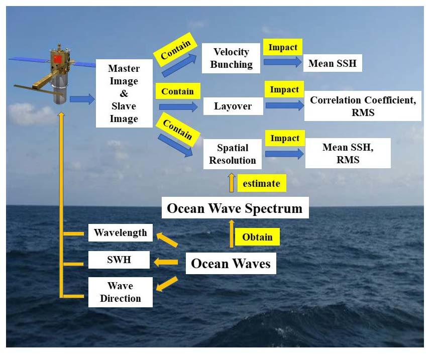
:The National Laboratory for Marine Science and Technology of China proposed the Guanlan ocean science satellite project in order to observe mesoscale and submesoscale ocean phenomena more effectively. In the project, the interferometric radar altimeter (IRA) is a main payload to be used to retrieve sea surface height (SSH) by means of interferometric imaging technology. Sea state is one of the important factors that affect the accuracy of the SSH that is retrieved by IRA. In the present work, the effects of velocity bunching and layover induced by sea waves are numerically simulated. The results demonstrate that the SSH would be significantly underestimated due to velocity bunching. On the other hand, the layover effect of sea waves along range direction would decrease (destroy) the coherence between the master-slave IRA images and then increase the random altimetry noise. Spatial smoothing is one of the main methods for reducing the residual error of sea waves. Here, we propose a theoretical formula to evaluate the residual error of sea waves for different wavelength, significant wave height and wave direction. The conclusions obtained in this work are helpful for better understanding the influence of sea state on the SSH retrieved by IRA.

1. Introduction
Since the advent of ocean radar satellite in the 1970s [1], altimeter and synthetic aperture radar (SAR) are two important microwave sensors for sea surface measurement. However, the spatial-temporal resolution of the traditional altimeter is poor, so the mesoscale and submesoscale ocean phenomena cannot be effectively observed [2]. Rodriguez et al. proposed a new sensor scheme of interferometric radar altimeter (IRA) in the wide-swath ocean altimeter (WSOA) mission. This scheme provides higher accuracy, better sampling, and observation of more phenomena [3,4]. NASA’s proposed Surface Water and Ocean Topography (SWOT) [5,6,7,8] mission will carry the Ka band Radar Interferometer (KaRIn) [9,10,11,12] in order to implement the IRA concept. A dual-frequency (Ku and Ka) IRA was designed for the Guanlan science mission of the National Laboratory for Marine Science and Technology of China [13]. SWOT and Guanlan aim to capture more ocean phenomena by accurately observing sea surface height (SSH), which requires strict control of measurement errors.
From the traditional altimeter to the IRA, sea state bias (SSB) [14], as one of the main errors in SSH measurement, has been influencing the accuracy of SSH measurement. For traditional altimeter, SSH measurement error research has been more comprehensive and in-depth. IRA contains the characteristics of both interferometric SAR (InSAR) and altimeter sensors; therefore, the SSH measurement error is more complicated. In recent years, a lot of research has been carried out on the errors of IRA, including the analysis of atmosphere media error [15,16,17], random error [18,19,20,21], and instrument systematic error [10,22]. Among these errors, ocean wave is one of the important factors that affect the SSH measurement, and the related research work is not comprehensive enough. In the general process of SAR observation, since the significance wave height (SWH) is small and the incident angle is large, the main factor that affects the SSH measurement is velocity bunching; however, the layover effect of ocean wave can be ignored. However, IRA has the same imaging mechanism as SAR, but with a smaller incident angle. Therefore, in addition to the effect of velocity bunching, the effect of overlaying is also significant. For traditional altimeter, the echo waveform is mainly affected by the distribution of sea scatterers in the footprint, which makes the distance measurement value of altimeter increase towards the direction of trough [14], and it also leads to the SSH deviation. Different from the traditional altimeter, the IRA measures SSH through the interference phase. The resolution of the measured data needs to reach the magnitude of kilometers and the effect of wave smoothing also needs to be considered in order to observe mesoscale and submesoscale ocean phenomena. From the above, we can see that the impact of ocean waves on the IRA height measurement results is mainly caused by the velocity bunching effect [23,24,25], the layover effect [26,27,28,29,30] caused by the small incident angle and the spatial resolution.
The sea surface scatterers with the radial velocity component in the IRA image will be offset along the azimuth direction due to the Doppler frequency shift of the radar echo, which is the velocity bunching, due to the IRA and the XT-InSAR having the same working mechanism. Much previous work has studied the mapping between the ocean wave orbital velocity and azimuthal displacement, and analyzed the impact of velocity bunching to the ocean wave inversion [31,32,33,34]. From these ocean wave inversion studies based on SAR imaging, it can be seen that velocity bunching will cause significant ocean waves distortion in the image. This distortion is related to the incident angle, wave height, wavelength, and wave direction. Yoshida studied the SAR imaging mechanism of waves moving along the azimuth through numerical simulation, and pointed out that when the azimuth shift caused by the maximum orbital motion was close to one quarter of the wavelength of the azimuthal wave, the wavelike pattern is more likely to appear [35]. Schulz-stellenfleth et al. calculated the bunched digital elevation model (DEM) by using the wave phase image of airborne X-band horizontally polarized XT-InSAR near the North Sea, and proposed a new method for calculating the modulation transfer function of real aperture radar by using the bunched DEM and the registered SAR intensity image [36]. The above researches focus more on the influence of velocity bunching on the ocean wave spectrum. Moreover, the phase and height distortion caused by velocity bunching will also affect the measurement of SSH. The IRA’s main mission is to measure the SSH, which requires high accuracy. The relevant work on this error is not perfect and it needs to be further carried out.
When compared with velocity bunching, the layover is also related to the incident angle, wave height, wavelength, and wave direction, which mainly causes the range direction displacement relative to the actual ocean surface position in the image. The displacement caused by layover is significant due to the small incident angle of IRA, which will affect the interference phase and reduce the correlation between the master-slave images. Previous researches have explained the reasons for layover from the SAR imaging mechanism, including Ulaby [26] and Rodriguez et al. [27]. Because the height of ocean surface fluctuation is small and most previous studies on SAR were conducted at medium or large incident angles, the effect of layover could be ignored. However, the layover must be considered, because the IRA incident angle is small. Peral et al. made some analysis on the layover in [28], and gave some quantitative results of layover based on KaRIn designed in the SWOT project. Dubois and Chapron provided a comprehensive description and discussed the implications of different factors of the SSB in the IRA [29].
Finally, in addition to the influence of the above two nonlinear effects, the spatial resolution is also an important factor to the SSH measurement. The final measurement results need to be smoothed, so that the spatial resolution reaches the magnitude of kilometers, in order to reduce the influence of random noise to effectively observe mesoscale and submesoscale ocean phenomena. The effect of waves smoothing, especially the swell with long wavelength, cannot be ignored. There are few relevant studies presently and in-depth analysis is needed.
According to the above studies, these three effects distort and cause significant influence of SSH measurement. The research on these effects is not enough at present, and further analysis is needed. Based on the Guanlan mission, this paper analyzes three influencing factors: velocity bunching, layover, and spatial resolution through simulation analysis. In the simulation of sea surface scattering field, the azimuthal displacement caused by velocity bunching and the range displacement caused by layover are considered. The effects of spatial resolution were studied by smoothing the simulated sea surface by combining theory with simulation analysis, including the original linear sea surface, the added velocity bunching sea surface, and the added layover sea surface. The simulation results verify the correctness of the theory. The main content of this paper is divided into four parts. Section 2 introduces the electromagnetic model and the principle of interference imaging used in simulation. Section 3 introduces velocity bunching and its simulation results. Section 4 introduces the layover and its simulation results. Section 5 introduces the influence of spatial resolution on the inversion results.
2. Electromagnetic Scattering Model and Interference Imaging Principle
A dual-frequency IRA is designed for Guanlan mission and it includes the wavelengths for the Ku and Ka bands. The Ku band is designed to cover an incident angle from 1° to 5.5°, while the Ka band from 4.5° to 6°, forming an overlapped region between 4.5° and 5.5° [12]. The geometrical optics model is selected in the simulation of scattering coefficient and scattering field, because it is a more practical method at low incident angle [37]. The normalized radar cross section (NRCS) can be expressed as
where is the local incident angle and is defined as the angle between wind direction and the azimuth direction. is the Fresnel coefficient at normal incidence on the surface at rest. and are the mean square slope (mss) of the x-axis and y-axis, respectively. The NRCS can be used to obtain the scattering field. However, there are two hypotheses that we should pay attention to before we get the scattering field. The first one is that the NRCS varies a little over the SAR illumination time [37]. This hypothesis has been used in [38] and [39]. The second one is that the complex reflectivity of spatially separated sea surface elements are mutually uncorrelated [40]. This hypothesis has been confirmed in [41] by experiment. The complex scattering field can be generated by random numbers that are based on these two hypotheses
where is the complex circular Gaussian random number, its expectation is 0, and its variance is the NRCS . The scattering field at each pixel in the master IRA image, regardless of velocity bunching and layover is obtained by (3), and according to (4), the slave image scattering field can be obtained by adding the determined interference phase difference to the master image scattering field
where is the wavenumber and . x is the azimuth direction, z is the direction perpendicular to the scattering plane, and y is orthogonal to x and z. is the range from the antenna to the pixel center, is the azimuthal position of the pixel center, and represent the range from the antenna to the scatterers, is the coefficient that depends on the system parameters, and is the range difference between antenna 1 and 2. is the intrinsic range resolution and is the IRA azimuth resolution. The interference phase difference between the master-slave image should be obtained by the interference imaging principle.
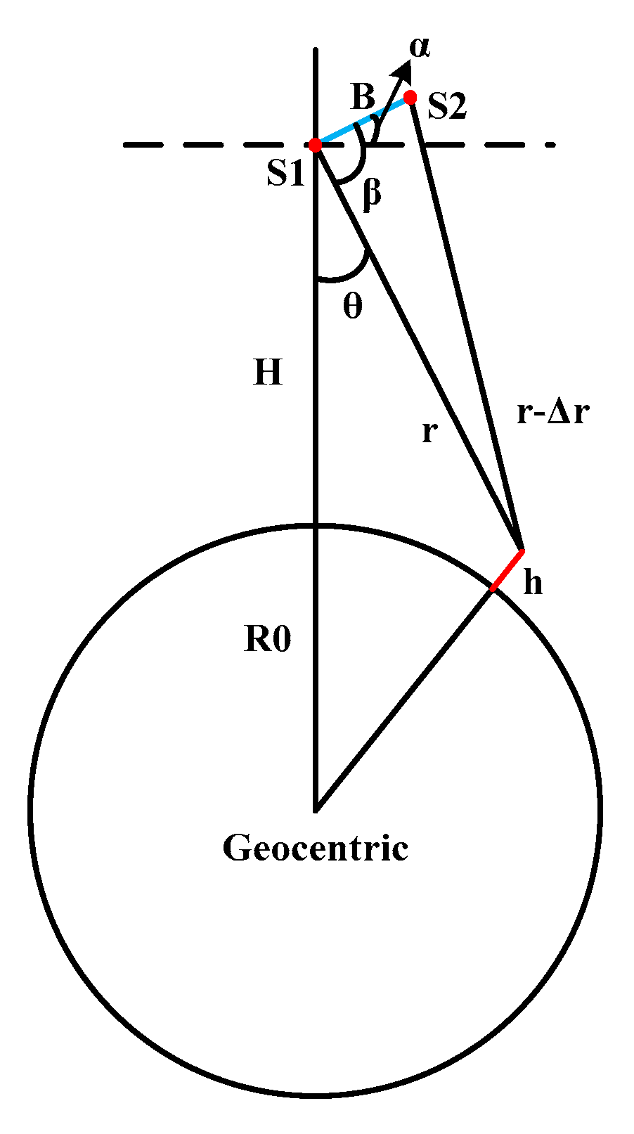
As shown in Figure 1, the interference principle of IRA is similar to the interference SAR (InSAR) [34]:
where is the range difference between antenna 1 and antenna 2 to the target and denotes the wavelength of the incident microwave. The range between them is calculated to obtain and by simulating satellite antenna coordinates and scatterers coordinates.
The phase difference includes flat phase and elevation phase, . The flat phase is the phase difference caused by the change of range with constant height. It is the main factor that causes the dense fringe in the interferometric phase diagram, as shown in (6)
where is the change of range, is the baseline length, is the incident angle, is the baseline angle, and is the range between the antenna and the scatterers. Removing the flat phase from , the result is a phase difference due to the change in SSH. The phase that is caused by the elevation can be expressed as:
where is the height relative to the sea surface. Accordingly, the can be calculated according to the following formula
If we want to obtain the SSH, according to the geometric relationship in Figure 1, the formula is
where is the included angle between the baseline and range of antenna 1, is the orbital height of the platform, is the radius of the earth, and is the height relative to the reference ellipsoid. The calculated results of (11) is the height relative to the reference ellipsoid.
We simulated the linear sea surface scattering field when the incident angle is 1° by combining with Guanlan satellite parameters. In this paper, the Monte Carlo method is used for sea surface simulation. However, only swells are retained in order to clearly study the phenomena caused by velocity bunching and layover. In the simulation process, the included angle between the swell propagation direction and radial direction of radar is the swell propagation direction angle. When the swell propagates along the range direction, the angle is 0°, and when the swell propagates along the azimuth direction, the angle is 90°. Table 1 shows the simulation parameters.
3. The Influence of Velocity Bunching
IRA is very sensitive to radial motion of the sea surface scatterers, which is similar to the SAR. As described in the introduction, velocity bunching is an inherent imaging mechanism of IRA, owing to the orbital velocity of waves [24]. It depends on the wave propagation direction, SWH, and wavelength, causing a nonlinear displacement in the azimuth.
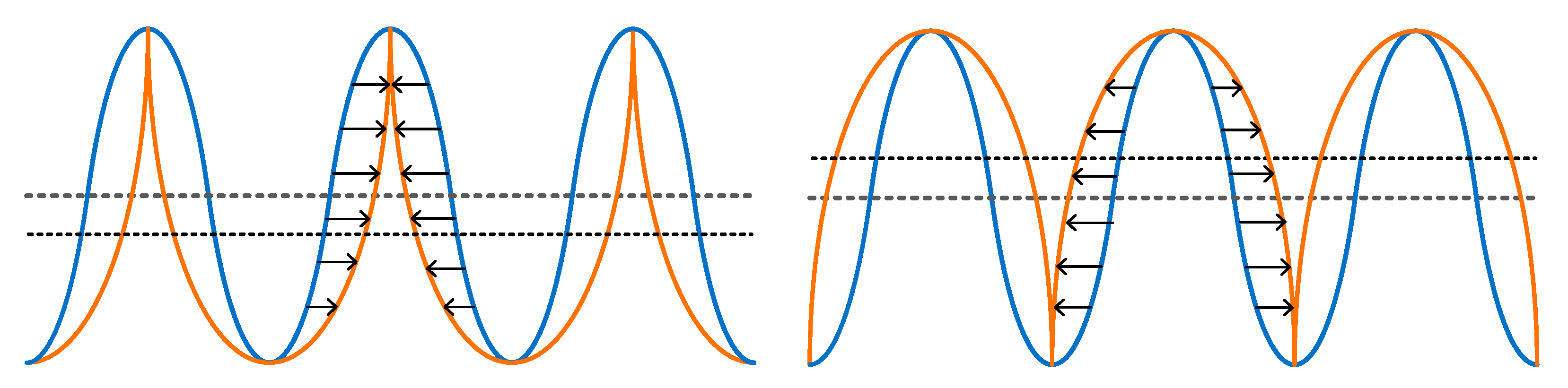
Figure 2 shows that the velocity bunching will cause strong nonlinear effects on the sea surface, resulting in the aggregation, dispersion, and even crossing of sea surface scatterers. Especially, the nonlinear displacement caused by velocity bunching will seriously influence the shape of waves in the IRA image when waves travel along the azimuth direction. It makes the peaks sharper and the troughs wider or the troughs sharper and the peaks wider, which depends on whether the waves velocity is towards or away from the platform. This will eventually cause bias in the inversion height.
According to the theory of velocity bunching, the projection of wave orbital velocity on the radial direction will cause the surface scatterers to offset in the azimuth, and the displacement can be expressed as
where is the range from the radar to the surface scattering element, is the flight velocity of the platform, and is the radial velocity component of the wave. The displacement and distorted position of each point caused by velocity bunching can be obtained from (12), and then the sea surface scattering field with velocity bunching effect can be obtained by superimposing the scattering field of corresponding displacement points.
As we know, the calculation of complex correlation coefficient between master-slave images can be expressed as
where S1 and S2 are the master and slave images scattering fields, respectively. The calculation of correlation coefficients in all simulation results in this paper is based on (13).
However, when choosing the smoothing window size, we try to choose the azimuth pixels to average rather than the range direction pixels. The scattering field of each scatterer in the master and slave images can be expressed as
where and are the phases generated by the distance between antenna and sea surface scatterers, while , . and are the random phase, which are uniformly distributed between -π and π, . Thus, in theory, if averaging an infinite number of scatterers, the random phases cancel each other out. In the actual processing, if the number of the average scatterers is small and the random phases cannot cancel each other, a large random noise will be generated and the inversion result will be affected. Therefore, enough scatterers should be selected in order to reduce the impact caused by the random phase. However, the flat phase expressed as (6) is worth noting when we are smoothing. We know that, in the obtained data, the flat phase changes periodically along the range direction, which is the reason for the fringe in the interference image. If we selected many smoothing scatterers in the range direction, the influence of the flat phase will be introduced into the elevation phase, which will bring a large error. Section 5 describes theoretical analysis of smoothing in detail.
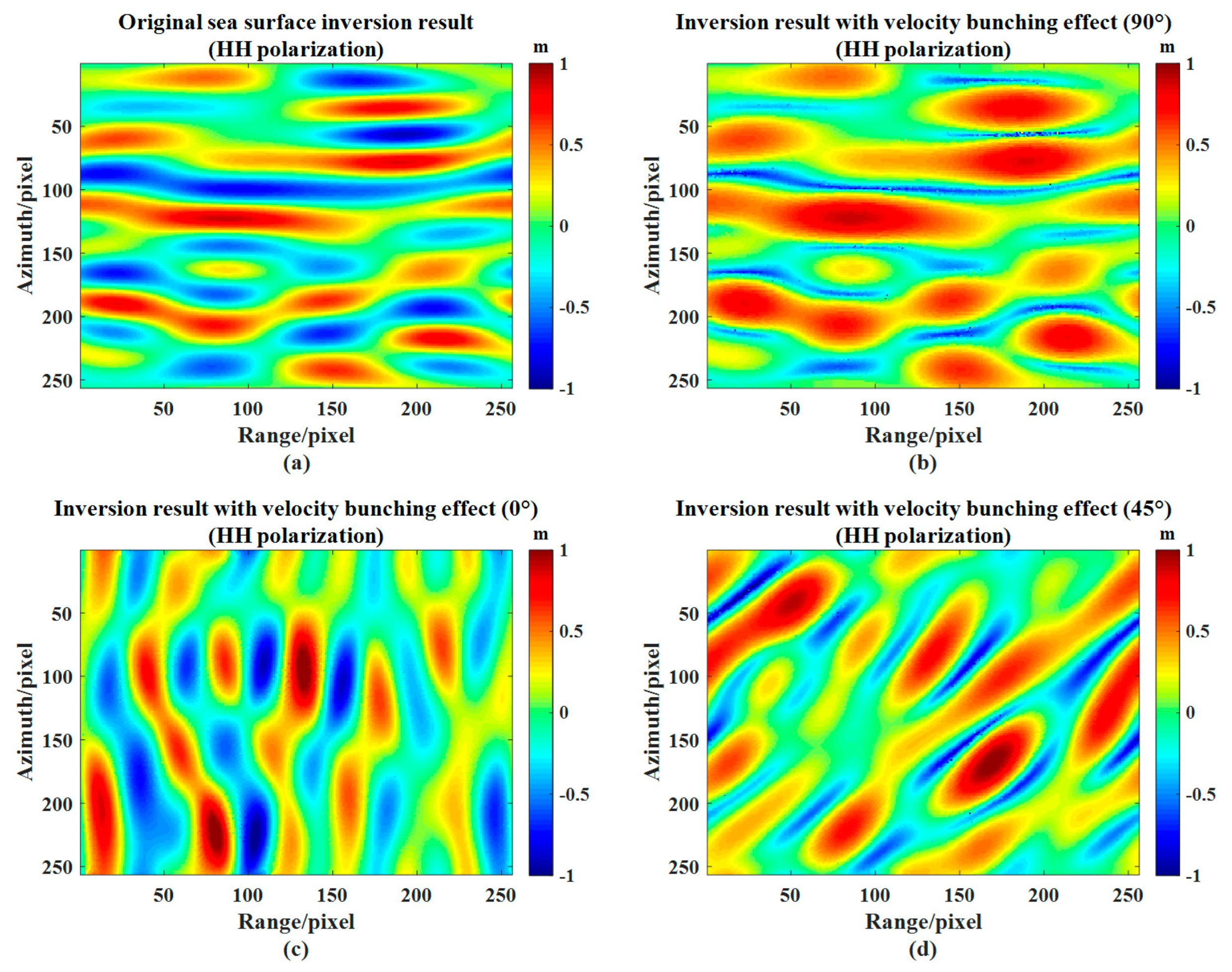
Swells have been chosen in different propagation directions, SWH, and wavelength in order to fully demonstrate the influence of velocity bunching. All the pixels along the azimuth direction are selected to be averaged when calculating the correlation coefficient. Figure 3 shows the comparison between the original sea surface and the added velocity bunching sea surface, as well as the velocity bunching of the swell in different propagation directions. The peaks become wider and the troughs become narrower (Figure 3a,b), which is dependent on the relative motion of the swell and the platform. This is also consistent with the theoretical analysis. Moreover, Figure 3b–d show that the damage of velocity bunching to SSH is the most serious when the swell propagation direction is 90° to the range direction. This also makes the inversion of the mean SSH results appear a large bias.
The correlation coefficient between the master and slave images does not change, because the correlation coefficient is also calculated by selecting the average of all pixels along the azimuth direction, as shown in Table 2, Table 3, and Table 4. The deviation of scatterers caused by velocity bunching only occurred in the azimuth direction, and the average number of scatterers is equal to the original sea surface. Thus, the correlation coefficient does not change. However, the inversion of SSH produces a large error owing to the distortion of sea surface caused by velocity bunching, which is expressed by the main SSH.
Table 2 shows the influence of velocity bunching under different swell propagation directions when SWH is 2 m and wavelength is 200 m. It is easy to see that the influence of velocity bunching reaches the maximum when the swell propagates at 90°. The sea surface distortion caused by the velocity bunching will cause a deviation of 0.156 m in the inversion SSH. This is equivalent to the SSH that is caused by mesoscale and submesoscale ocean phenomena, which seriously affects the identification of ocean phenomena. However, velocity bunching has little effect on root mean square (RMS).
The swell propagation direction is 90° in order to demonstrate the effects of velocity bunching under different SWH and different wavelength conditions. Table 3 gives the influence results of velocity bunching under different SWH. The higher the SWH is, the greater the impact of velocity bunching is, and the maximum SSH deviation can reach 0.588 m, and even the minimum is 4 cm. This has seriously obscured the height of the ocean phenomena observed.
Table 4 shows the influence of velocity bunching at different wavelengths. Similarly, the propagation direction of 90° and the SWH of 2 m are selected. The SSH deviation that is caused by velocity bunching decreases with the increase of wavelength. This is because the displacement distance of the scatterers caused by the velocity bunting is smaller than the wavelength, which causes less damage to the sea surface and reduces the error.
Thus, the effect caused by velocity bunching is closely related to propagation direction, SWH, and wavelength when the satellite orbital height and flight speed are fixed. If the displacement caused by velocity bunching is large and the troughs are not squeezed but crossed, the mean height might not change much.
4. The Influence of Layover
Layover is called the “range-bunching effect” [42] in the SAR Ocean Imaging theory and the “surfboard sampling” [28] in the imaging process of the wide-swath imaging altimeter. Its main effect is to distort the sea surface in the range direction, so that the points on the same wavefront in the range direction will offset or overlap (shown in Figure 4). For small incident angles, such as 1°, according to (7), 1 m SSH will offset the sea surface scatterer by about 57 m. This is more than 10 resolution units away from the 5 m ground resolution. However, in the actual situation, the scattering field of one point is the superposition of many scatterers due to the fixed range resolution and poor ground resolution at near range. Therefore, the height distortion in the inversion result cannot be obviously obtained, while the correlation coefficient will significantly decrease.
The correlation reflects the level of random phase noise in the interference phase between master and slave image. The random phase noise will affect the final height inversion result. The layover will introduce the effect of flat phase in the range direction, which will have great impact on the inversion results. Therefore, we analyze the volumetric decorrelation that is caused by layover. We assume that enough pixels along the azimuth are selected to be averaged, and then the SWH in the average region satisfies the Gaussian probability function,
where is the height relative to the mean sea surface and is the standard deviation of . The elevation phase can be expressed as (7), so the volumetric decorrelation due to the SSH can be given by [27]:
Combining Guanlan parameter, according to (16), we can obtain the volumetric correlation coefficient within the whole incident angle, where the Ku band is selected for the whole swath.
The near range correlation is poor, but it is still above 0.975, and the correlation difference of near range and far range is not much, as shown in Figure 5. SWH also affects the correlation, the larger the SWH, the worse the correlation.
In order to fully demonstrate the influence of layover, swells have also chosen different propagation directions, SWH and wavelength. All of the pixels along the azimuth are also selected to be averaged when calculating the correlation coefficient.
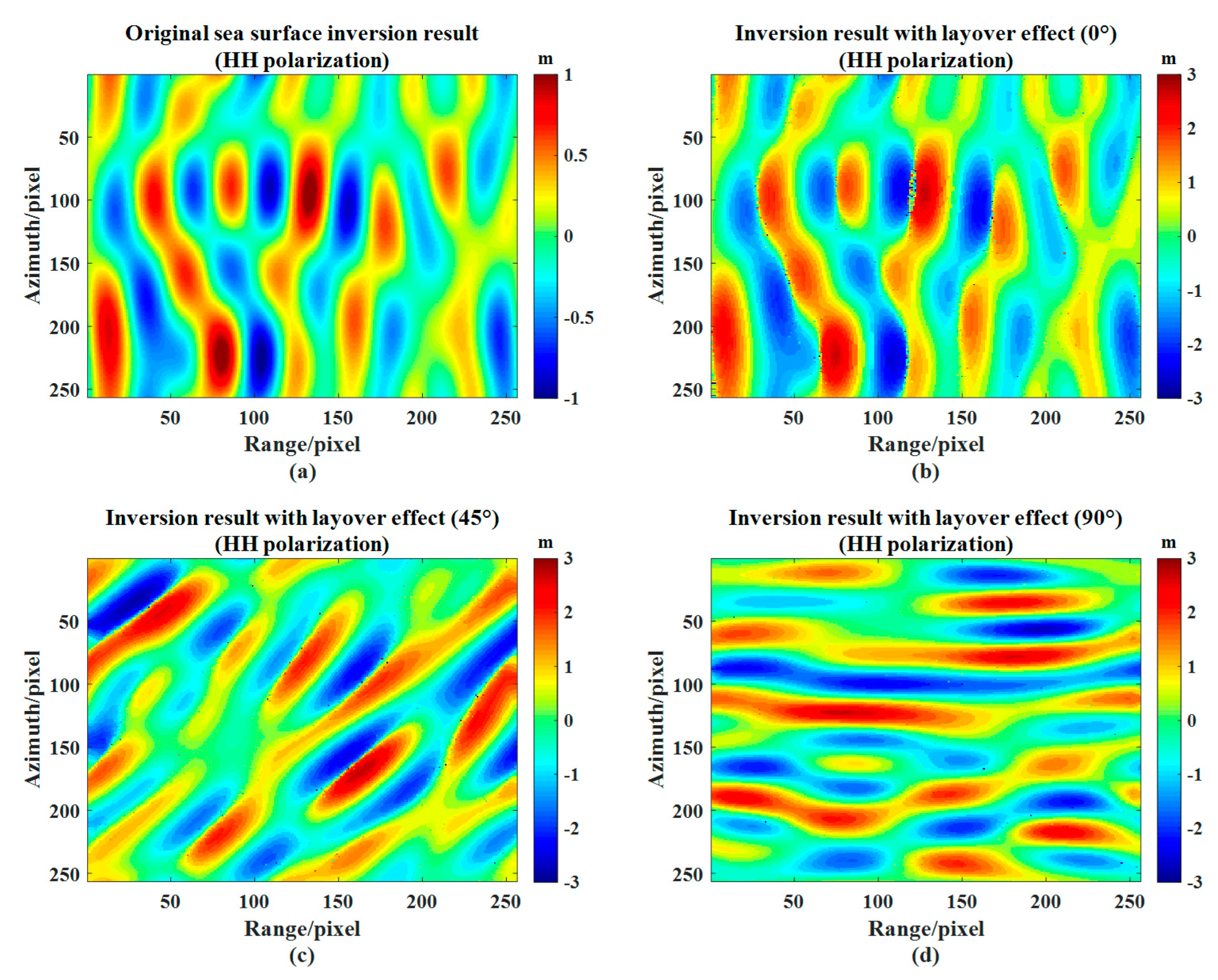
Figure 6 shows the comparison between the original sea surface and the added layover sea surface, as well as the layover of the swell in different propagation directions. Figure 6a,b illustrate that the wavefront and waveback have significant squeezing and stretching. This also agreed with the theoretical analysis. In addition, Figure 6b–d exhibit that the damage of layover to SSH is the most serious when the swell propagation direction is 0°.
Table 5 shows the influence of layover under different swell propagation directions when SWH is 2 m and wavelength is 200 m. The mean SSH deviation due to the layover, although on the order of centimeter, is much smaller than that due to the velocity bunching. This is attributed to layover making the sea surface scatterers move to the reference plane of height 0, rather than changing the scatterers distribution of wave peaks and troughs. However, the RMS increases significantly, which is caused by the random phase effect of the scatterers superimposed on the same sampling plane. The correlation coefficient between the master and slave images also decreased slightly, which was basically consistent with the theoretical results. The propagation direction has little influence on the error and correlation coefficient of layover inversion results, while it is still not negligible for mesoscale and submesoscale centimeter-level fluctuations.
The swell propagation direction is 0° in order to show the effects of layover under different SWH and wavelength conditions. Table 6 gives the influence results of layover under different SWH. The deviation that is caused by layover is sensitive to the change of SWH. When SWH is 5 m, the mean SSH of the inversion results will be reduced by 4 cm, and even with the 3 m SWH common in the ocean, the deviation will reach nearly 3 cm. Although SWH will reduce the correlation coefficient more than the propagation direction, it still remains above 0.960, which has little impact on the correlation of master-slave images.
Table 7 shows the influence of layover at different wavelengths. Similarly, the propagation direction of 0° and the SWH of 2 m are selected. The influence of wavelength on the inversion results is not significant. The reason is the same as the effect of SWH. The mean SSH and correlation coefficient are basically unchanged.
Therefore, SWH is the important factor affecting the mean SSH deviation of layover inversion. This also agreed with the formation mechanism of layover, which is essentially caused by the SSH being in the same radar sampling plane.
5. The Influence of Spatial Resolution
As we know, smoothing processing is one of the effective methods for eliminating the random noise of IRA image and improving the image correlation. In the processing of interference phase, we also need to carry out smoothing processing to reduce the random phase noise and improve the interference between master and slave image. However, we need to be careful with phase filtering. The elevation obtained by inversion can be processed in smoothing processing in order to avoid introducing the influence of flat phase in the range direction. The spatial resolution after smoothing processing is similar to low-pass filtering. Ignoring the effects of velocity bunching and layover, the ideal SSH inversion results can be obtained. Smoothing on this basis will still bring some errors.
The influence of spatial resolution on inversion results can be quantitatively expressed. Taking the monochromatic wave as an example, it can be given by
When considering the influence of spatial resolution, (17) can be written as [43]:
where the wavenumber are and , in which and are the lengths of the ocean surface along range and azimuth directions. and are the spatial resolution of the radar along range and azimuth directions. We define the spatial damping coefficient related to spatial resolution as [44]:
It reflects the variation of correlation coefficient in spatial resolution. However, it is easy to ignore that the smoothing process itself will bring errors when smoothing the inversion results.
For real sea surface simulation, we can use the Lagrange wave model, so the ocean surface can be simulated by [43]:
where represents the position of each point on the ocean surface, is the Fourier coefficient of the ocean surface, and the angular frequency is . The result after smoothing can be expressed as:
Thus, the RMS of theoretically smooth sea surface can be expressed as:
represents the ocean wave spectrum corresponding to the simulated ocean surface.
If wind wave is ignored and swell is only considered, the mean value of SSH obtained is strictly 0 only when the smoothing window is equal to an integer multiple of the wavelength of the swell, owing to ocean waves being essentially the superposition of many sine waves with different frequencies and amplitudes. The error is maximum when the smoothing window is half of the wavelength. However, the error tends to converge when the smoothing window increases.
Firstly, the monochromatic wave is taken as an example for analysis. Figure 7 demonstrates the variation of smoothing error with wavelength and smoothing window size. During the simulation, the pixel size is set to 5 m × 5 m and the smoothing window is a square window. The included angle between wave propagation direction and X-axis is 0°. The residual error is larger when the size of the smoothing window is smaller than the wave wavelength. The error oscillation decreases and finally tends to converge when the window is gradually larger. Therefore, the smoothing window itself will bring errors to the inversion result without the distortion of wave shape caused by velocity bunching and layover. Moreover, the error cannot be ignored for centimeter-level fluctuations of mesoscale and submesoscale ocean phenomena.
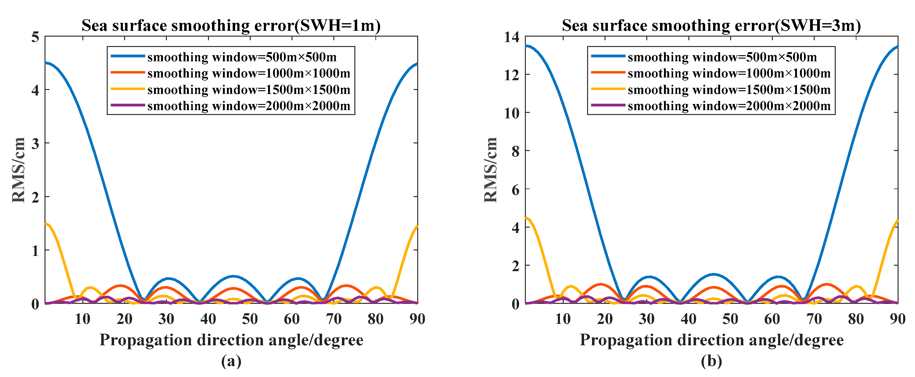
Figure 8 shows the relationship between the smoothing error and wave propagation direction when the wave wavelength and the smoothing window size is fixed. In the simulation, we set the wave wavelength at 200 m, the propagation direction at 0° to 90° to the range direction, and the size of the smoothing window at 500 m, 1000 m, 1500 m, and 2000 m, respectively. Moreover, in addition to the influence of wave propagation direction on the smoothing error, the relationship between the size of the smoothing window and the wavelength also has a great influence on the smoothing error. (a) The smoothing error oscillates with the propagation direction, because the wavelength components that are projected in the azimuth and range directions change during the propagation direction change. The error is minimized when the size of the smoothing window is an integer multiple of the projected component and the error is maximized when the smoothing window is 0.5 times larger than the projected component and it contains the least swell period. (b) In the case of 0° and 90° to the range direction, the influence of the relationship between the smoothing window and wavelength on the error can be clearly seen. Large errors occur when the wave period contained in the smoothing window is not an integer multiple. The above two points illustrate that the smoothing window and wave propagation direction have significant influence on the smoothing error.
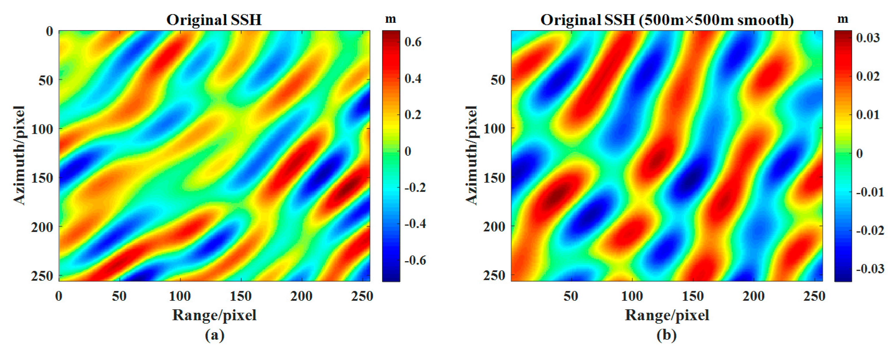
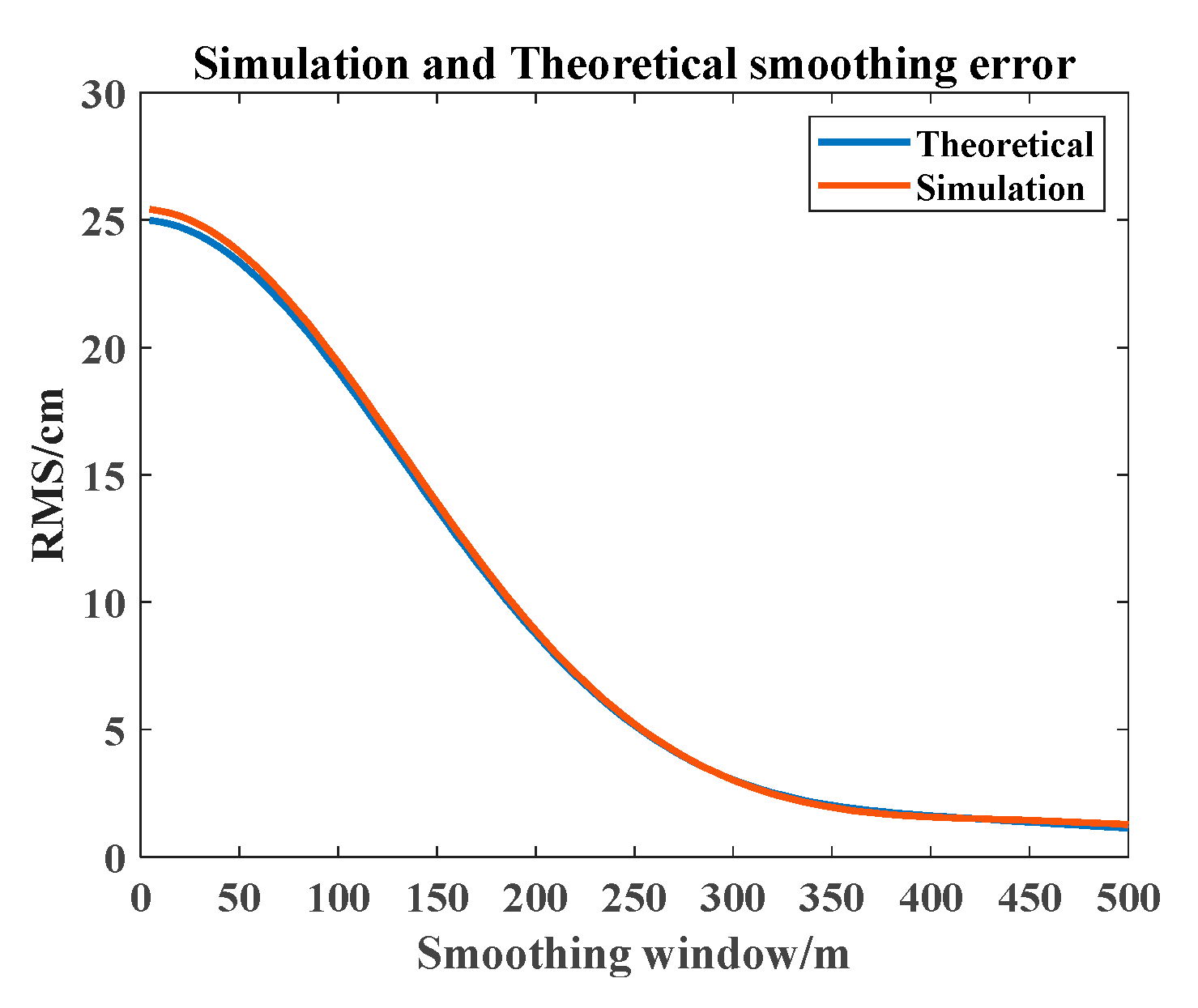
In addition to monochromatic waves, we also study the simulated real sea surface. Figure 9 demonstrates the two-dimensional sea surface simulation results without smoothing and after smoothing. The SWH is selected as 2 m, the smoothing window size is 500 m × 500 m, and the pixel size is 5 m × 5 m. The sea surface that is simulated in Figure 9a is smoothed, and the result is compared with the theoretical results calculated by (22), which are in good agreement with each other. Figure 9 indicates that the SSH has decreased and the shape of the swell has changed after smoothing.
The results presented in Figure 10 are in good agreement with the theory shown in (22), which effectively verifies the accuracy of the theory. The variation of spatial resolution is an error term in the SSH measurement, which reflects the influence of waves on the measurement results. For the spatial resolution error of the global sea area, there is no need to obtain the SSH, only the ocean wave spectrum of the determined location at the determined time can be obtained, and the error can be quantified by (22).
The variation of sea surface smoothing error with propagation direction is also given. The curve does not change in oscillation and the error is smaller than that of monochromatic wave simulation results, as shown in Figure 11a. The real sea surface swell is formed by the superposition of multiple monochromatic waves, and each monochromatic wave has a different wavelength, so it has different sensitivity to the smoothing window. Figure 11b illustrates the smoothing error increases with the increase of wavelength when SWH and smooth window are fixed. This result means that different wavelengths have different sensitivities to smooth window. Figure 11c shows the variation of smoothing error with SWH. In the same smoothing window, the higher the SWH, the greater the smoothing error. Figure 11 shows that the propagation direction, SWH, and wavelength of ocean waves are all important factors affecting the smoothing error. The error is significant, which is similar to the fluctuation of mesoscale and submesoscale ocean phenomena, and will affect the observation of ocean phenomena.
In addition to influence of the size of the smoothing window on the inversion results, the direction that is selected by the smoothing window also has a great influence on the inversion results. The effects of waves need to be removed in order to study mesoscale and submesoscale oceanic phenomena. If smooth processing is carried out in the height field, in the case of enough smoothing pixels, theoretically, the smoothing window should be parallel to the swell propagation direction. Thus, the peaks and troughs can cancel each other to the maximum extent and eliminate the influence of waves. However, the real waves are not spread along the same direction and their wavelengths are not fixed due to the superposition of multiple waves. Therefore, the actual processing of the wave smoothing window should a rectangular window, in the order of kilometers, and it needs to be large enough to filter out high frequency signals that influence mesoscale and the submesoscale low frequency signal.
The residual error after smoothing is obtained by smoothing the simulated SSH presented in Section 3. The deviation of the mean SSH does not change due to the smoothing. Only the RMS is discussed here to illustrate the influence of waves on the smoothing result. Table 8 lists the RMS of smoothing velocity bunching inversion results with different swell propagation directions. The smoothing effect of a rectangular smoothing window is better than that of a unidirectional window, and the residual error is closely related to the propagation direction. Therefore, for the smoothing of the height data with unknown propagation direction, the rectangular smoothing window should be selected in order to minimize the impact of waves.
Table 9 lists the change of RMS with SWH. Under the same smoothing window, the residual error increases with the increase of SWH. The residual error is basically in the order of millimeters when the smoothing window is 1 km × 1 km. Table 10 shows the change of RMS with wavelength. The residual error depends on whether the number of wavelengths contained in the smoothing window is an integer or not. This also agrees with the theoretical analysis.
For layover, the simulation results in Section 4 are smoothed in the same way as the velocity bunching. The deviation of the mean SSH also does not change owing to the smoothing. Table 11 is the RMS of smoothing layover inversion results with different swell propagation directions. The results are similar to those presented in Table 8. The difference is that the residual error after the smoothing of the layover is greater than the velocity bunching.
Table 12 and Table 13 show the change of RMS with SWH and wavelength, respectively. The results cannot be compared with the results of velocity bunching because of the different propagation directions. However, the layover will increase the influence of waves on the inversion results by analyzing the velocity bunching smoothing results and the layover smoothing results, including the influence of random phase after the superposition of scatterers.
Combining the height smoothing results of velocity bunching and layover: (a) for the height smoothing, the smoothing window should be a rectangular window. Therefore, we can guarantee the window to cross the wave period and achieve a better smoothing effect in the case of unknown propagation direction. (b) The smoothing window should be expanded on the premise of ensuring the effective display of mesoscale and submesoscale ocean signals, so as to reduce the influence of SWH and wavelength on RMS and reduce the influence of waves.
For phase filtering, the selection of smoothing window needs to be more careful. Figure 12 shows the phase changes that are caused by SSH changes at near and far range. The 1 m height change results in a phase change of only about 0.2 rad compared with the flat phase variation of 2π at near range. The elevation phase variation is much smaller than the flat phase variation. Therefore, assuming that the two antennas is strictly side-looking, if the smoothing is along the azimuth direction, the smoothing window can be as large as possible, because the same azimuth direction to the flat phase is the same and it will not introduce the influence of the flat phase. If the smoothing is along the range direction, then the change of flat phase will mask the elevation phase, introducing a large error. In principle, the range direction smoothing pixels should not be chosen. However, in actual satellite-borne or airborne imaging process, the interference fringe will be inclined due to the change in the flight attitude of the platform. Subsequently, the smoothing along the azimuth direction would not be parallel to the direction of the interference fringe and the influence of flat phase will still be introduced. The smoothing window should be chosen to be parallel to the interference fringe and fewer smoothing pixels should be chosen in the direction perpendicular to the fringe when processing an interference image.
We also smoothed the phase image. For velocity bunching, the smoothing analysis of phase image is also carried out. The smoothing of the phase images is different from that of layover. Since layover is related to SAR imaging mechanism, the inversion result can be calculated according to (8). However, because the effect of layover is not considered in the process of velocity bunching simulation, the inversion result should follow (23)
The height is a change with respect to the reference point directly below, not on the same sampling plane. Therefore, under the same height, the phase change is times that when layover is considered, and the effect of flat phase on the inversion height is magnified by times. Moreover, the phase change also shows that the flat phase and the random phase caused by the superposition of scatterers have great influence on the inversion results. This results in a huge error in the inverse performance of (23). However, for the real situation, the influence of the flat phase and the random phase is ultimately reflected in the inversion results through (8). The results presented in Table 14, Table 15 and Table 16 correspond to the real situation.
Table 14, Table 15 and Table 16 show a common theme that azimuthal smoothing in phase reduces the error to the millimeter level. However, the error can grow to tens of centimeters or even meters with range smoothing. This is unacceptable in the measurement results. This also fully shows that the flat phase has great influence on the phase smoothing process.
Table 14 shows that the RMS will oscillate when the propagation direction changes. On the one hand, it is related to the velocity bunching; on the other hand, whether the smoothing window crosses the flat phase period is also an important factor. Similarly, in Table 15, the RMS of the rectangular window and the window along the range will increase with the increase of SWH when the smoothing window is 0.5 km. This is because the window does not cross the flat phase period. The RMS oscillates again when the window crosses the period. The results presented in Table 16 oscillate because of the effect of flat phase.
In the same way, we smooth the interference phase of the layover and analyze the inversion height of the smoothed phase. Table 17, Table 18 and Table 19 list that the layover will make the wave’s influence on the inversion result increase (the maximum approach to 1 m) after azimuth smoothing. This is mainly caused by the random phase effect after the scatterers are superimposed. The RMS increases dramatically to about 14 m when range smoothing is added. The RMS reaches 1 m at the 0.5 km window without crossing the flat phase period. These results all include the effect of flat phase due to the smoothing processing.
Combining the phase smoothing results of velocity bunching and layover: (a) for phase smoothing, the smoothing window should be selected along the azimuth direction, so as to avoid the influence of flat phase and obtain a better smoothing result. However, for the actual data, the azimuth direction is not parallel to the interference fringe due to the instability of the platform’s flight attitude. Therefore, in the actual data processing, the smoothing window should choose the direction parallel to the interference fringe and avoid choosing the smoothing unit perpendicular to the fringe. (b) Large smoothing window is conducive to reducing RMS, so, in the case of clear mesoscale and submesoscale ocean signals, the smoothing window should be enlarged to reduce the impact of waves.
6. Conclusions
In this paper, the effects of velocity bunching, layover, and spatial resolution on IRA inversion results are studied. The results show that the layover mainly affects the correlation of master-slave images and the effect of interference imaging, while the velocity bunching more affects the mean SSH inversion. For different sea conditions and system parameters, layover and velocity bunching have different effects.
For the spatial resolution, if the smoothing is carried out in the height image, it will still bring bias to the inversion result without the influence of velocity bunching and layover. However, if the phase image is smoothed, the flat phase will have great influence on the inversion results.
In the actual height smoothing, we hope to choose the rectangular smoothing window of the magnitude of kilometers to reduce the impact of waves, while the mean SSH deviation that is caused by the velocity bunching and layover cannot be eliminated. In actual phase smoothing, we suggest that the smooth window should be parallel to the interference fringe, and the window should avoid crossing the fringe to reduce the effect of flat phase. Moreover, the error cannot be completely eliminated, owing to the window being selected for infinite size, which is also related to the wave period. The process can minimize the impact of waves on the observation of mesoscale and submesoscale ocean phenomena. In addition, we can also estimate the impact of waves on the inversion results after smoothing by combining buoy or forecast data to obtain the ocean wave spectrum of the region of study.
In future work, we hope to systematize the relationship between error and nonlinear effect, and study and discuss the influence of nonlinear sea surface and wind wave.
Author Contributions
Conceptualization, C.Z. and G.C.; Data curation, Y.B.; Formal analysis, C.Z.; Funding acquisition, Y.W.; Methodology, Y.B. and Y.W.; Resources, G.C.; Writing-original draft, Y.B.; Writing-review & editing, Y.W. and Y.Z. All authors have read and agreed to the published version of the manuscript.
Funding
This research was funded by the Marine S & T Fund of Shandong Province for Pilot National Laboratory for Marine Science and Technology (Qingdao) under Grant No.2018SDKJ0102-8., key research and development program of Shandong Province (International Science and technology cooperation), No.2019GHZ023. and the National Natural Science Foundation of China (41576170, 41976167).
Conflicts of Interest
The authors declare no conflict of interest.
References
- Fu, L.; Chelton, D.B.; Le Traon, P.; Morrow, R. Eddy dynamics from satellite altimetry. Oceanography 2010, 23, 14–25. [Google Scholar] [CrossRef] [Green Version]
- Pascual, A.; Faugère, Y.; Larnicol, G.; Le Traon, P.Y. Improved description of the ocean mesoscale variability by combining four satellite altimeters. Geophys. Res. Lett. 2006, 33, L02611. [Google Scholar] [CrossRef] [Green Version]
- Rodriguez, E.; Pollard, B.; Martin, J. Wide-swath ocean altimetry using radar interferometry. IEEE Trans. Geosci. Remote Sens. 1999, 37, 624–626. [Google Scholar]
- Enjolras, V.; Vincent, P.; Souyris, J.; Rodriguez, E.; Phalippou, L.; Cazenave, A. Performances study of interferometric radar altimeters: From the instrument to the global mission definition. Sensors 2006, 6, 164–192. [Google Scholar] [CrossRef] [Green Version]
- Fu, L.; Alsdorf, D.; Morrow, R.; Rodriguez, E.; Mognard, N. SWOT: The Surface Water and Ocean Topography Mission: Wide-swath Altimetric Elevation on Earth; No. JPL-Publication 12–05; Jet Propulsion Laboratory: Pasadena, CA, USA, 2012.
- Durand, M.; Fu, L.; Lettenmaier, D.P.; Alsdorf, D.E.; Rodriguez, E.; Esteban-Fernandez, D. The surface water and ocean topography mission: Observing terrestrial surface water and oceanic submesoscale eddies. Proc. IEEE 2010, 98, 766–779. [Google Scholar] [CrossRef]
- Vaze, P.; Kaki, S.; Limonadi, D.; Esteban-Fernandez, D.; Zohar, G. The Surface Water and Ocean Topography Mission; IEEE: Piscataway, NJ, USA, 2018; pp. 1–9. [Google Scholar]
- Fu, L.; Ubelmann, C. On the transition from profile altimeter to swath altimeter for observing global ocean surface topography. J. Atmos. Ocean. Tech. 2014, 31, 560–568. [Google Scholar] [CrossRef]
- Esteban-Fernandez, D.; Fu, L.; Rodriguez, E.; Brown, S.; Hodges, R. Ka-band SAR interferometry studies for the SWOT mission. In Proceedings of the 2010 IEEE International Geoscience and Remote Sensing Symposium, Honolulu, HI, USA, 25–30 July 2010; IEEE: Piscataway, NJ, USA, 2010; pp. 4401–4402. [Google Scholar]
- Gawande, R.; Tope, M.; Michalik, M.; Baldi, C.; Pak, K.; Esteban-Fernandez, D. Ka-band Phase Measurement System for SWOT mission. In 2019 URSI Asia-Pacific Radio Science Conference (AP-RASC); IEEE: Piscataway, NJ, USA, 2019; pp. 1–3. [Google Scholar]
- Fjørtoft, R.; Gaudin, J.; Pourthie, N.; Lion, C.; Mallet, A.; Souyris, J.; Ruiz, C.; Koudogbo, F.; Duro, J.; Ordoqui, P. KaRIn-the Ka-band radar interferometer on SWOT: Measurement principle, processing and data specificities. In Proceedings of the 2010 IEEE International Geoscience and Remote Sensing Symposium, Honolulu, HI, USA, 25–30 July 2010; IEEE: Piscataway, NJ, USA, 2010; pp. 4823–4826. [Google Scholar]
- Fjørtoft, R.; Gaudin, J.; Pourthie, N.; Lalaurie, J.; Mallet, A.; Nouvel, J.; Martinot-Lagarde, J.; Oriot, H.; Borderies, P.; Ruiz, C. KaRIn on SWOT: Characteristics of near-nadir Ka-band interferometric SAR imagery. IEEE Trans. Geosci. Remote Sens. 2013, 52, 2172–2185. [Google Scholar] [CrossRef]
- Chen, G.; Tang, J.; Zhao, C.; Wu, S.; Yu, F.; Ma, C.; Xu, Y.; Chen, W.; Zhang, Y.; Liu, J. Concept Design of the “Guanlan” Science Mission: China’s Novel Contribution to Space Oceanography. Front. Mar. Sci. 2019, 6, 194. [Google Scholar] [CrossRef] [Green Version]
- Chelton, D.; Ries, J.; Haines, B.; Fu, L.; Callahan, P. Satellite Altimetry, in Satellite Altimetry and Earth Sciences: A Handbook of Techniques and Applications; Fu, L., Cazenave, A., Eds.; Academic Press: San Diego, CA, USA, 2001; pp. 1–131. [Google Scholar]
- Mercier, F.; Rosmorduc, V.; Carrere, L.; Thibaut, P. Coastal and Hydrology Altimetry Product (PISTACH) Handbook; Centre National d’Études Spatiales (CNES): Paris, France, 2010; p. 4. [Google Scholar]
- Gairola, R.M.; Pokhrel, S.; Varma, A.K.; Agarwal, V.K. A combined passive–active microwave retrieval of quantitative rainfall from Topex/Poseidon radar altimeter and Topex microwave radiometer. Int. J. Remote Sens. 2005, 26, 1729–1753. [Google Scholar] [CrossRef]
- Ubelmann, C.; Fu, L.; Brown, S.; Peral, E.; Esteban-Fernandez, D. The effect of atmospheric water vapor content on the performance of future wide-swath ocean altimetry measurement. J. Atmos. Ocean. Tech. 2014, 31, 1446–1454. [Google Scholar] [CrossRef]
- Oliver, C.; Quegan, S. Understanding Synthetic Aperture Radar Images; Artech House: Boston, MA, USA, 1998. [Google Scholar]
- Lee, J. Speckle suppression and analysis for synthetic aperture radar images. Opt. Eng. 1986, 25, 255636. [Google Scholar] [CrossRef]
- Kuan, D.T.; Sawchuk, A.A.; Strand, T.C.; Chavel, P. Adaptive noise smoothing filter for images with signal-dependent noise. IEEE Trans. Pattern Anal. 1985, 165–177. [Google Scholar] [CrossRef]
- Frost, V.S.; Stiles, J.A.; Shanmugan, K.S.; Holtzman, J.C. A model for radar images and its application to adaptive digital filtering of multiplicative noise. IEEE Trans. Pattern Anal. 1982, 157–166. [Google Scholar] [CrossRef]
- Li, Z.; Wang, J.; Fu, L.L. An observing system simulation experiment for ocean state estimation to assess the performance of the SWOT mission: Part 1—A twin experiment. J. Geophys. Res. Oceans 2019, 124, 4838–4855. [Google Scholar] [CrossRef]
- Alpers, W.; Rufenach, C.L. The effect of orbital motions on synthetic aperture radar imagery of ocean waves. IEEE Trans. Antenn. Propag. 1979, 27, 685–690. [Google Scholar] [CrossRef]
- Alpers, W.R.; Ross, D.B.; Rufenach, C.L. On the detectability of ocean surface waves by real and synthetic aperture radar. J. Geophys. Res. Oceans 1981, 86, 6481–6498. [Google Scholar] [CrossRef]
- Hasselmann, K.; Raney, R.K.; Plant, W.J.; Alpers, W.; Shuchman, R.A.; Lyzenga, D.R.; Rufenach, C.L.; Tucker, M.J. Theory of synthetic aperture radar ocean imaging: A MARSEN view. J. Geophys. Res. Oceans 1985, 90, 4659–4686. [Google Scholar] [CrossRef]
- Ulaby, F.T.; Moore, R.K.; Fung, A.K. Microwave Remote Sensing: Active and Passive. Volume 2-Radar Remote Sensing and Surface Scattering and Emission Theory; Artech House, Inc.: Norwood, MA, USA, 1982. [Google Scholar]
- Rodriguez, E.; Martin, J.M. Theory and design of interferometric synthetic aperture radars. IEE Proc. Radar Signal Process. 1992, 139, 147–159. [Google Scholar] [CrossRef]
- Peral, E.; Rodríguez, E.; Esteban-Fernández, D. Impact of surface waves on SWOT’s projected ocean accuracy. Remote Sens. 2015, 7, 14509–14529. [Google Scholar] [CrossRef] [Green Version]
- Dubois, P.; Chapron, B. Characterization of the ocean waves signature to assess the Sea State Bias in wide-swath interferometric altimetry. In Proceedings of the IGARSS 2018–2018 IEEE International Geoscience and Remote Sensing Symposium, Valencia, Spain, 22–27 July 2018; IEEE: Piscataway, NJ, USA, 2018; pp. 3789–3792. [Google Scholar]
- Rosen, P.A.; Hensley, S.; Joughin, I.R.; Li, F.K.; Madsen, S.N.; Rodriguez, E.; Goldstein, R.M. Synthetic aperture radar interferometry. Proc. IEEE. 2000, 88, 333–382. [Google Scholar] [CrossRef]
- Bao, M.; Alpers, W.; Bruning, C. A new nonlinear integral transform relating ocean wave spectra to phase image spectra of an along-track interferometric synthetic aperture radar. IEEE Trans. Geosci. Remote Sens. 1999, 37, 461–466. [Google Scholar]
- He, Y.; Alpers, W. On the nonlinear integral transform of an ocean wave spectrum into an along-track interferometric synthetic aperture radar image spectrum. J. Geophys. Res. Oceans 2003, 108, 3205. [Google Scholar] [CrossRef]
- Bao, M. A nonlinear integral transform between ocean wave spectra and phase image spectra of a cross-track interferometric SAR. In Proceedings of the IEEE 1999 International Geoscience and Remote Sensing Symposium. IGARSS’99 (Cat. No.99CH36293), Hamburg, Germany, 28 June–2 July 1999; IEEE: Piscataway, NJ, USA, 1999; Volume 5, pp. 2619–2621. [Google Scholar]
- Schulz-Stellenfleth, J.; Lehner, S. Ocean wave imaging using an airborne single pass across-track interferometric SAR. IEEE Trans. Geosci. Remote Sens. 2001, 39, 38–45. [Google Scholar] [CrossRef]
- Yoshida, T. Numerical research on clear imaging of azimuth-traveling ocean waves in SAR images. Radio Sci. 2016, 51, 989–998. [Google Scholar] [CrossRef] [Green Version]
- Schulz-Stellenfleth, J.; Horstmann, J.; Lehner, S.; Rosenthal, W. Sea surface imaging with an across-track interferometric synthetic aperture radar: The SINEWAVE experiment. IEEE Trans. Geosci. Remote Sens. 2001, 39, 2017–2028. [Google Scholar] [CrossRef]
- Boisot, O.; Nouguier, F.; Chapron, B.; Guérin, C. The GO4 model in near-nadir microwave scattering from the sea surface. IEEE Trans. Geosci. Remote Sens. 2015, 53, 5889–5900. [Google Scholar] [CrossRef] [Green Version]
- Bao, M.; Bruning, C.; Alpers, W. Simulation of ocean waves imaging by an along-track interferometric synthetic aperture radar. IEEE Trans. Geosci. Remote Sens. 1997, 35, 618–631. [Google Scholar]
- Plant, W.J. Reconciliation of theories of synthetic aperture radar imagery of ocean waves. J. Geophys. Res. Oceans 1992, 97, 7493–7501. [Google Scholar] [CrossRef]
- Liu, B.; He, Y. SAR raw data simulation for ocean scenes using inverse Omega-K algorithm. IEEE Trans. Geosci. Remote Sens. 2016, 54, 6151–6169. [Google Scholar] [CrossRef]
- Plant, W.J.; Schuler, D.L. Remote sensing of the sea surface using one-and two-frequency microwave techniques. Radio Sci. 1980, 15, 605–615. [Google Scholar] [CrossRef]
- Chapron, B.; Johnsen, H.; Garello, R. Wave and wind retrieval from SAR images of the ocean. Springer 2001, 56, 682–699. [Google Scholar]
- Donelan, M.A.; Anctil, F.; Doering, J.C. A simple method for calculating the velocity field beneath irregular waves. Coast. Eng. 1992, 16, 399–424. [Google Scholar] [CrossRef]
- Wang, Y.; Li, H.; Zhang, Y.; Guo, L. The measurement of sea surface profile with X-band coherent marine radar. Acta Oceanol. Sin. 2015, 34, 65–70. [Google Scholar] [CrossRef]
Figure 1.
Schematic of the interferometric radar altimeter (IRA) geometry.

Figure 2.
Conceptual illustration of velocity bunching. The blue curve is the ‘real’ monochromatic wave height, the orange curve is the effect of velocity bunching. The gray dash line is the original mean sea surface height (SSH), the black dash line is the mean SSH with velocity bunching.
Figure 2.
Conceptual illustration of velocity bunching. The blue curve is the ‘real’ monochromatic wave height, the orange curve is the effect of velocity bunching. The gray dash line is the original mean sea surface height (SSH), the black dash line is the mean SSH with velocity bunching.

Figure 3.
Simulation results of original sea surface (a) and added velocity bunching sea surface (in m). The swell propagation direction is 90° (b), 0° (c), and 45° (d) to the range direction.
Figure 3.
Simulation results of original sea surface (a) and added velocity bunching sea surface (in m). The swell propagation direction is 90° (b), 0° (c), and 45° (d) to the range direction.

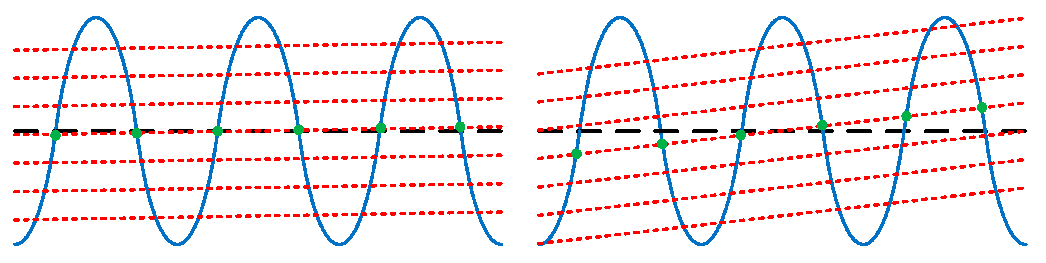
Figure 4.
Conceptual illustration of layover. The two pictures are the schematic diagram when the incident angle is 1° (left) and 7° (right), respectively. The blue curve is the ‘real’ monochromatic wave height, the red dash line is the wavefront of the radar beam, and the green dots are the sea surface scattering elements on the same wavefront. The black dash line is the original mean SSH. That means all the green points will overlap into the same point during the imaging process, resulting in distortion of the sea surface.

Figure 5.
Volumetric decorrelation varies with incident angle and SWH.

Figure 6.
Simulation results of original sea surface (a) and added layover sea surface (in m). The swell propagation direction is 0° (b), 45° (c), and 90° (d) to the range direction.
Figure 6.
Simulation results of original sea surface (a) and added layover sea surface (in m). The swell propagation direction is 0° (b), 45° (c), and 90° (d) to the range direction.

Figure 7.
Effect of smoothing window on monochromatic waves of different wavelengths (in cm). The SWH is selected as 1 m (a) and 3 m (b), the wave direction is 0° and the pixel size is 5 m × 5 m. The smoothing window is a square window. (c,d) are the magnification of the smooth window results from 500 m to 2000 m in (a) and (b), respectively.

Figure 8.
Effect of propagation angle on monochromatic waves (in cm). The SWH is selected as 1 m (a) and 3 m (b), the wave wavelength is 200 m and the pixel size is 5 m × 5 m. The smoothing window is a square window.
Figure 8.
Effect of propagation angle on monochromatic waves (in cm). The SWH is selected as 1 m (a) and 3 m (b), the wave wavelength is 200 m and the pixel size is 5 m × 5 m. The smoothing window is a square window.

Figure 9.
Unsmoothed (a) and smoothed (b) original SSH (in m). The SWH is selected as 2 m. The smoothing window size is 500 m × 500 m, and the pixel size is 5 m × 5 m.
Figure 9.
Unsmoothed (a) and smoothed (b) original SSH (in m). The SWH is selected as 2 m. The smoothing window size is 500 m × 500 m, and the pixel size is 5 m × 5 m.

Figure 10.
Original sea surface smoothing error (in cm). The SWH is selected as 2 m and the pixel size is 5 m × 5 m. The smoothing window is a square window.
Figure 10.
Original sea surface smoothing error (in cm). The SWH is selected as 2 m and the pixel size is 5 m × 5 m. The smoothing window is a square window.

Figure 11.
Influence of propagation direction, wavelength and SWH on smoothing error (in cm). The pixel size is 5 m × 5 m. The smoothing window is (a) square window. The incident angle in (b) and (c) is set to 0°.
Figure 11.
Influence of propagation direction, wavelength and SWH on smoothing error (in cm). The pixel size is 5 m × 5 m. The smoothing window is (a) square window. The incident angle in (b) and (c) is set to 0°.

Figure 12.
Change in elevation phase at near and far range (in rad). The blue line shows the change of phase with elevation when the incident angle is 1°, and the red line shows the change of phase with elevation when the incident angle is 7°.
Figure 12.
Change in elevation phase at near and far range (in rad). The blue line shows the change of phase with elevation when the incident angle is 1°, and the red line shows the change of phase with elevation when the incident angle is 7°.


Table 1.
System simulation parameters.
| System Simulation Parameters | Values |
|---|---|
| Altitude | 900 km |
| Physical baseline length | 12 m |
| Center frequency | Ku band |
| Polarization | HH |
| Swell wavelength | 200 m |
| Swell height | 1 m |
| Incident angle | 1° |
| Azimuth resolution | 5 m |
| Ground range resolution | 5 m |
Table 2.
The influence of velocity bunching under different swell propagation directions (the significance wave height (SWH) is 2 m, the wavelength is 200 m).
Table 2.
The influence of velocity bunching under different swell propagation directions (the significance wave height (SWH) is 2 m, the wavelength is 200 m).
| Direction | Parameter | Original | Velocity Bunching |
|---|---|---|---|
| 0° | Mean height/m | 0 | 0 |
| RMS/m | 0.354 | 0.354 | |
| Correlation coefficient | 1 | 1 | |
| 30° | Mean height/m | 0 | 0.099 |
| RMS/m | 0.353 | 0.339 | |
| Correlation coefficient | 1 | 1 | |
| 45° | Mean height/m | 0 | 0.098 |
| RMS/m | 0.353 | 0.337 | |
| Correlation coefficient | 1 | 1 | |
| 60° | Mean height/m | 0 | 0.128 |
| RMS/m | 0.353 | 0.330 | |
| Correlation coefficient | 1 | 1 | |
| 90° | Mean height/m | 0 | 0.156 |
| RMS/m | 0.353 | 0.330 | |
| Correlation coefficient | 1 | 1 |
Table 3.
The influence of velocity bunching under different SWH (the propagation direction is 90°, the wavelength is 200 m).
Table 3.
The influence of velocity bunching under different SWH (the propagation direction is 90°, the wavelength is 200 m).
| SWH | Parameter | Original | Velocity Bunching |
|---|---|---|---|
| 1 m | Mean height/m | 0 | 0.040 |
| RMS/m | 0.177 | 0.173 | |
| Correlation coefficient | 1 | 1 | |
| 2 m | Mean height/m | 0 | 0.156 |
| RMS/m | 0.353 | 0.324 | |
| Correlation coefficient | 1 | 1 | |
| 3 m | Mean height/m | 0 | 0.321 |
| RMS/m | 0.530 | 0.478 | |
| Correlation coefficient | 1 | 1 | |
| 5 m | Mean height/m | 0 | 0.588 |
| RMS/m | 0.884 | 0.977 | |
| Correlation coefficient | 1 | 1 |
Table 4.
The influence of velocity bunching under different swell wavelength (the propagation direction is 90°, the SWH is 2 m).
Table 4.
The influence of velocity bunching under different swell wavelength (the propagation direction is 90°, the SWH is 2 m).
| Wavelength | Parameter | Original | Velocity Bunching |
|---|---|---|---|
| 100 m | Mean height/m | 0 | 0.199 |
| RMS/m | 0.353 | 0.431 | |
| Correlation coefficient | 1 | 1 | |
| 200 m | Mean height/m | 0 | 0.156 |
| RMS/m | 0.353 | 0.324 | |
| Correlation coefficient | 1 | 1 | |
| 300 m | Mean height/m | 0 | 0.079 |
| RMS/m | 0.353 | 0.347 | |
| Correlation coefficient | 1 | 1 |
Table 5.
The influence of layover under different swell propagation directions (the SWH is 2 m, the wavelength is 200 m).
Table 5.
The influence of layover under different swell propagation directions (the SWH is 2 m, the wavelength is 200 m).
| Direction | Parameter | Original | Layover |
|---|---|---|---|
| 0° | Mean height/m | 0 | −0.024 |
| RMS/m | 0.354 | 1.039 | |
| Correlation coefficient | 1 | 0.993 | |
| 30° | Mean height/m | 0 | −0.021 |
| RMS/m | 0.353 | 1.049 | |
| Correlation coefficient | 1 | 0.991 | |
| 45° | Mean height/m | 0 | −0.019 |
| RMS/m | 0.353 | 1.046 | |
| Correlation coefficient | 1 | 0.991 | |
| 60° | Mean height/m | 0 | −0.016 |
| RMS/m | 0.353 | 1.054 | |
| Correlation coefficient | 1 | 0.991 | |
| 90° | Mean height/m | 0 | −0.007 |
| RMS/m | 0.353 | 1.059 | |
| Correlation coefficient | 1 | 0.991 |
Table 6.
The influence of layover under different SWH (the propagation direction is 0°, the wavelength is 200 m).
Table 6.
The influence of layover under different SWH (the propagation direction is 0°, the wavelength is 200 m).
| SWH | Parameter | Original | Layover |
|---|---|---|---|
| 1 m | Mean height/m | 0 | −0.011 |
| RMS/m | 0.177 | 0.532 | |
| Correlation coefficient | 1 | 0.998 | |
| 2 m | Mean height/m | 0 | −0.024 |
| RMS/m | 0.354 | 1.039 | |
| Correlation coefficient | 1 | 0.993 | |
| 3 m | Mean height/m | 0 | −0.028 |
| RMS/m | 0.530 | 1.480 | |
| Correlation coefficient | 1 | 0.985 | |
| 5 m | Mean height/m | 0 | −0.042 |
| RMS/m | 0.884 | 2.128 | |
| Correlation coefficient | 1 | 0.960 |
Table 7.
The influence of layover under different wavelength (the propagation direction is 0°, the SWH is 2 m).
Table 7.
The influence of layover under different wavelength (the propagation direction is 0°, the SWH is 2 m).
| Wavelength | Parameter | Original | Layover |
|---|---|---|---|
| 100 m | Mean height/m | 0 | −0.020 |
| RMS/m | 0.353 | 0.905 | |
| Correlation coefficient | 1 | 0.992 | |
| 200 m | Mean height/m | 0 | −0.024 |
| RMS/m | 0.354 | 1.039 | |
| Correlation coefficient | 1 | 0.993 | |
| 300 m | Mean height/m | 0 | −0.019 |
| RMS/m | 0.353 | 1.053 | |
| Correlation coefficient | 1 | 0.994 |
Table 8.
The root mean square (RMS) of smoothing velocity bunching height inversion results with different swell propagation directions (the direction of the smoothing window is in two directions at the same time, in the azimuth and in the range).
Table 8.
The root mean square (RMS) of smoothing velocity bunching height inversion results with different swell propagation directions (the direction of the smoothing window is in two directions at the same time, in the azimuth and in the range).
| Direction | 0.5 km × 0.5 km | 0.5 km × 5 m | 5 m × 0.5 km | 1 km × 1 km | 1 km × 5 m | 5 m × 1 km |
|---|---|---|---|---|---|---|
| 0° | 0.035 m | 0.252 m | 0.051 m | 0.010 m | 0.250 m | 0.021 m |
| 30° | 0.041 m | 0.142 m | 0.075 m | 0.005 m | 0.045 m | 0.043 m |
| 45° | 0.043 m | 0.138 m | 0.077 m | 0.005 m | 0.051 m | 0.046 m |
| 60° | 0.056 m | 0.091 m | 0.118 m | 0.009 m | 0.048 m | 0.036 m |
| 90° | 0.056 m | 0.089 m | 0.267 m | 0.007 m | 0.028 m | 0.241 m |
Table 9.
The RMS of smoothing velocity bunching height inversion results with different significance wave height (SWH) (the direction of the smoothing window is in two directions at the same time, in the azimuth and in the range).
Table 9.
The RMS of smoothing velocity bunching height inversion results with different significance wave height (SWH) (the direction of the smoothing window is in two directions at the same time, in the azimuth and in the range).
| SWH | 0.5 km × 0.5 km | 0.5 km × 5 m | 5 m × 0.5 km | 1 km × 1 km | 1 km × 5 m | 5 m × 1 km |
|---|---|---|---|---|---|---|
| 1 m | 0.022 m | 0.031 m | 0.150 m | 0.003 m | 0.008 m | 0.140 m |
| 2 m | 0.056 m | 0.089 m | 0.267 m | 0.007 m | 0.028 m | 0.241 m |
| 3 m | 0.086 m | 0.146 m | 0.369 m | 0.009 m | 0.062 m | 0.310 m |
| 5 m | 0.112 m | 0.204 m | 0.625 m | 0.021 m | 0.132 m | 0.548 m |
Table 10.
The RMS of smoothing velocity bunching height inversion results with different wavelength (the direction of the smoothing window is in two directions at the same time, in the azimuth and in the range).
Table 10.
The RMS of smoothing velocity bunching height inversion results with different wavelength (the direction of the smoothing window is in two directions at the same time, in the azimuth and in the range).
| Wavelength | 0.5 km × 0.5 km | 0.5 km × 5 m | 5 m × 0.5 km | 1 km × 1 km | 1 km × 5 m | 5 m × 1 km |
|---|---|---|---|---|---|---|
| 100 m | 0.015 m | 0.054 m | 0.144 m | 0.014 m | 0.038 m | 0.093 m |
| 200 m | 0.056 m | 0.089 m | 0.267 m | 0.007 m | 0.028 m | 0.241 m |
| 300 m | 0.093 m | 0.123 m | 0.328 m | 0.019 m | 0.058 m | 0.143 m |
Table 11.
The RMS of smoothing layover height inversion results with different swell propagation directions (the direction of the smoothing window is in two directions at the same time, in the azimuth and in the range).
Table 11.
The RMS of smoothing layover height inversion results with different swell propagation directions (the direction of the smoothing window is in two directions at the same time, in the azimuth and in the range).
| Direction | 0.5 km × 0.5 km | 0.5 km × 5 m | 5 m × 0.5 km | 1 km × 1 km | 1 km × 5 m | 5 m × 1 km |
|---|---|---|---|---|---|---|
| 0° | 0.088 m | 0.722 m | 0.132 m | 0.027 m | 0.680 m | 0.057 m |
| 30° | 0.054 m | 0.341 m | 0.158 m | 0.016 m | 0.096 m | 0.087 m |
| 45° | 0.051 m | 0.314 m | 0.160 m | 0.016 m | 0.092 m | 0.093 m |
| 60° | 0.052 m | 0.159 m | 0.333 m | 0.013 m | 0.067 m | 0.101 m |
| 90° | 0.112 m | 0.140 m | 0.931 m | 0.016 m | 0.034 m | 0.873 m |
Table 12.
The RMS of smoothing layover height inversion results with different SWH (the direction of the smoothing window is in two directions at the same time, in the azimuth and in the range).
Table 12.
The RMS of smoothing layover height inversion results with different SWH (the direction of the smoothing window is in two directions at the same time, in the azimuth and in the range).
| SWH | 0.5 km × 0.5 km | 0.5 km × 5 m | 5 m × 0.5 km | 1 km × 1 km | 1 km × 5 m | 5 m × 1 km |
|---|---|---|---|---|---|---|
| 1 m | 0.046 m | 0.377 m | 0.068 m | 0.014 m | 0.361 m | 0.031 m |
| 2 m | 0.088 m | 0.722m | 0.132 m | 0.027 m | 0.680 m | 0.057 m |
| 3 m | 0.121 m | 0.954 m | 0.192 m | 0.036 m | 0.829 m | 0.085 m |
| 5 m | 0.164 m | 1.092 m | 0.308 m | 0.050 m | 0.732 m | 0.118 m |
Table 13.
The RMS of smoothing layover height inversion results with different wavelength (the direction of the smoothing window is in two directions at the same time, in the azimuth and in the range).
Table 13.
The RMS of smoothing layover height inversion results with different wavelength (the direction of the smoothing window is in two directions at the same time, in the azimuth and in the range).
| Wavelength | 0.5 km × 0.5 km | 0.5 km × 5 m | 5 m × 0.5 km | 1 km × 1 km | 1 km × 5 m | 5 m × 1 km |
|---|---|---|---|---|---|---|
| 100 m | 0.026 m | 0.377 m | 0.072 m | 0.011 m | 0.310 m | 0.041 m |
| 200 m | 0.088 m | 0.722 m | 0.132 m | 0.027 m | 0.680 m | 0.057 m |
| 300 m | 0.140 m | 0.870 m | 0.167 m | 0.021 m | 0.841 m | 0.070 m |
Table 14.
The RMS of smoothing velocity bunching phase results with different swell propagation directions (the direction of the smoothing window is in two directions at the same time, in the azimuth and in the range).
Table 14.
The RMS of smoothing velocity bunching phase results with different swell propagation directions (the direction of the smoothing window is in two directions at the same time, in the azimuth and in the range).
| Direction | 0.5 km × 0.5 km | 0.5 km × 5 m | 5 m × 0.5 km | 1 km × 1 km | 1 km × 5 m | 5 m × 1 km |
|---|---|---|---|---|---|---|
| 0° | 0.143 m | 0.004 m | 0.723 m | 1.350 m | 0.003 m | 1.259 m |
| 30° | 0.138 m | 0.004 m | 0.902 m | 1.384 m | 0.002 m | 1.236 m |
| 45° | 0.156 m | 0.004 m | 0.930 m | 1.248 m | 0.002 m | 1.226 m |
| 60° | 0.157 m | 0.003 m | 1.287 m | 1.348 m | 0.003 m | 1.253 m |
| 90° | 0.187 m | 0.004 m | 1.749 m | 1.033 m | 0.003 m | 0.960 m |
Table 15.
The RMS of smoothing velocity bunching phase results with different SWH (the direction of the smoothing window is in two directions at the same time, in the azimuth and in the range).
Table 15.
The RMS of smoothing velocity bunching phase results with different SWH (the direction of the smoothing window is in two directions at the same time, in the azimuth and in the range).
| SWH | 0.5 km × 0.5 km | 0.5 km × 5 m | 5 m × 0.5 km | 1 km × 1 km | 1 km × 5 m | 5 m × 1 km |
|---|---|---|---|---|---|---|
| 1 m | 0.124 m | 0.004 m | 1.301 m | 1.105 m | 0.002 m | 1.156 m |
| 2 m | 0.187 m | 0.004 m | 1.749 m | 1.033 m | 0.003 m | 0.960 m |
| 3 m | 0.267 m | 0.004 m | 2.198 m | 1.000 m | 0.003 m | 0.925 m |
| 5 m | 0.305 m | 0.004 m | 2.487 m | 0.491 m | 0.002 m | 0.970 m |
Table 16.
The RMS of smoothing velocity bunching phase results with different wavelength (the direction of the smoothing window is in two directions at the same time, in the azimuth and in the range).
Table 16.
The RMS of smoothing velocity bunching phase results with different wavelength (the direction of the smoothing window is in two directions at the same time, in the azimuth and in the range).
| Wavelength | 0.5 km × 0.5 km | 0.5 km × 5 m | 5 m × 0.5 km | 1 km × 1 km | 1 km × 5 m | 5 m × 1 km |
|---|---|---|---|---|---|---|
| 100 m | 0.167 m | 0.003 m | 2.340 m | 1.252 m | 0.002 m | 0.986 m |
| 200 m | 0.187 m | 0.004 m | 1.749 m | 1.033 m | 0.003 m | 0.960 m |
| 300 m | 0.165 m | 0.003 m | 1.305 m | 0.923 m | 0.002 m | 0.959 m |
Table 17.
The RMS of smoothing layover phase results with different swell propagation directions (the direction of the smoothing window is in two directions at the same time, in the azimuth and in the range).
Table 17.
The RMS of smoothing layover phase results with different swell propagation directions (the direction of the smoothing window is in two directions at the same time, in the azimuth and in the range).
| Direction | 0.5 km × 0.5 km | 0.5 km × 5 m | 5 m × 0.5 km | 1 km × 1 km | 1 km × 5 m | 5 m × 1 km |
|---|---|---|---|---|---|---|
| 0° | 0.449 m | 0.473 m | 1.205 m | 15.694 m | 0.406 m | 14.312 m |
| 30° | 0.227 m | 0.218 m | 1.145 m | 14.559 m | 0.088 m | 14.607 m |
| 45° | 0.220 m | 0.205 m | 1.131 m | 12.343 m | 0.092 m | 14.559 m |
| 60° | 0.126 m | 0.136 m | 0.953 m | 14.436 m | 0.071 m | 14.655 m |
| 90° | 0.128 m | 0.139 m | 0.905 m | 12.582 m | 0.066 m | 14.876 m |
Table 18.
The RMS of smoothing layover phase results with different SWH (the direction of the smoothing window is in two directions at the same time, in the azimuth and in the range).
Table 18.
The RMS of smoothing layover phase results with different SWH (the direction of the smoothing window is in two directions at the same time, in the azimuth and in the range).
| SWH | 0.5 km × 0.5 km | 0.5 km × 5 m | 5 m × 0.5 km | 1 km × 1 km | 1 km × 5 m | 5 m × 1 km |
|---|---|---|---|---|---|---|
| 1 m | 0.251 m | 0.257 m | 0.862 m | 15.469 m | 0.244 m | 14.930 m |
| 2 m | 0.449 m | 0.473 m | 1.205 m | 15.694 m | 0.406 m | 14.312 m |
| 3 m | 0.607 m | 0.588 m | 1.500 m | 15.275 m | 0.409 m | 13.817 m |
| 5 m | 0.814 m | 0.995 m | 1.919 m | 14.788 m | 0.989 m | 13.646 m |
Table 19.
The RMS of smoothing layover phase results with different wavelength (the direction of the smoothing window is in two directions at the same time, in the azimuth and in the range).
Table 19.
The RMS of smoothing layover phase results with different wavelength (the direction of the smoothing window is in two directions at the same time, in the azimuth and in the range).
| Wavelength | 0.5 km × 0.5 km | 0.5 km × 5 m | 5 m × 0.5 km | 1 km × 1 km | 1 km × 5 m | 5 m × 1 km |
|---|---|---|---|---|---|---|
| 100 m | 0.294 m | 0.321 m | 1.292 m | 15.947 m | 0.197 m | 13.120 m |
| 200 m | 0.449 m | 0.473 m | 1.205 m | 15.694 m | 0.406 m | 14.312 m |
| 300 m | 0.563 m | 0.570 m | 1.039 m | 14.264 m | 0.537 m | 14.479 m |
© 2020 by the authors. Licensee MDPI, Basel, Switzerland. This article is an open access article distributed under the terms and conditions of the Creative Commons Attribution (CC BY) license (http://creativecommons.org/licenses/by/4.0/).
Share and Cite
MDPI and ACS Style
Bai, Y.; Wang, Y.; Zhang, Y.; Zhao, C.; Chen, G. Impact of Ocean Waves on Guanlan’s IRA Measurement Error. Remote Sens. 2020, 12, 1534. https://doi.org/10.3390/rs12101534
AMA Style
Bai Y, Wang Y, Zhang Y, Zhao C, Chen G. Impact of Ocean Waves on Guanlan’s IRA Measurement Error. Remote Sensing. 2020; 12(10):1534. https://doi.org/10.3390/rs12101534
Chicago/Turabian StyleBai, Yining, Yunhua Wang, Yanmin Zhang, Chaofang Zhao, and Ge Chen. 2020. "Impact of Ocean Waves on Guanlan’s IRA Measurement Error" Remote Sensing 12, no. 10: 1534. https://doi.org/10.3390/rs12101534
Note that from the first issue of 2016, this journal uses article numbers instead of page numbers. See further details here.