Satellite-Based Observations Reveal Effects of Weather Variation on Rice Phenology


1
Department of Environmental Science and Policy, University of California, Davis, CA 95616-8627, USA
2
International Center for Tropical Agriculture, Nairobi 823-00621, Kenya
3
Department of Plant Sciences, University of California, Davis, CA 95616-8627, USA
*
Author to whom correspondence should be addressed.
Remote Sens. 2020, 12(9), 1522; https://doi.org/10.3390/rs12091522
Submission received: 16 April 2020
/
Revised: 7 May 2020
/
Accepted: 8 May 2020
/
Published: 10 May 2020
(This article belongs to the Special Issue Remote and Proximal Assessment of Plant Traits)
Abstract
:Obtaining detailed data on the spatio-temporal variation in crop phenology is critical to increasing our understanding of agro-ecosystem function, such as their response to weather variation and climate change. It is challenging to collect such data over large areas through field observations. The use of satellite remote sensing data has made phenology data collection easier, although the quality and the utility of such data to understand agro-ecosystem function have not been widely studied. Here, we evaluated satellite data-based estimates of rice phenological stages in California, USA by comparing them with survey data and with predictions by a temperature-driven phenology model. We then used the satellite data-based estimates to quantify the crop phenological response to changes in weather. We used time-series of MODIS satellite data and PhenoRice, a rule-based rice phenology detection algorithm, to determine annual planting, heading and harvest dates of paddy rice in California between 2002 and 2017. At the state level, our satellite-based estimates of rice phenology were very similar to the official survey data, particularly for planting and harvest dates (RMSE = 3.8–4.0 days). Satellite based observations were also similar to predictions by the DD10 temperature-driven phenology model. We analyzed how the timing of these phenological stages varied with concurrent temperature and precipitation over this 16-year time period. We found that planting was earlier in warm springs (−1.4 days °C−1 for mean temperature between mid-April and mid-May) and later in wet years (5.3 days 100 mm-1 for total precipitation from March to April). Higher mean temperature during the pre-heading period of the growing season advanced heading by 2.9 days °C−1 and shortened duration from planting to heading by 1.9 days °C−1. The entire growing season was reduced by 3.2 days °C−1 because of the increased temperature during the rice season. Our findings confirm that satellite data can be an effective way to estimate variations in rice phenology and can provide critical information that can be used to improve understanding of agricultural responses to weather variation.
1. Introduction
Crop phenology, the timing of crop growth stages, is influenced by crop management and environmental conditions, particularly temperature [1,2,3]. Crop phenology plays an important role in determining crop yield [4,5,6]. It determines growing season length and the coincidence of phenological stages with stress events, for example heat stress during flowering, can also greatly affect crop yield [7,8]. Understanding crop phenology is thus of fundamental importance for the study and mitigation of adverse weather effects on crop production [9,10].
The physiological processes related to the effect of weather on crop phenology are well understood from experimental observations and modeling studies [11]. However, it is less clear how these processes play out in farmers’ fields over larger temporal and spatial scales [12]. The variation in phenology arises not only from the diverse environmental conditions under which crops are grown, but also from differences in crop management choices, such as the planting date and the crop variety selected [3,13,14,15]. Therefore, quantifying crop phenological development over space and time is important for understanding how variation in the weather affects crop development on farms.
Several computer models have been developed to predict crop phenology from weather data [16]. These can be stand-alone temperature (and sometimes photoperiod) driven phenology models, such as DD10 for rice [17,18] or more complex crop growth simulation models such as APSIM [19] or ORYZA [20]. These models are particularly useful to assess the expected crop response to changes in the environment or management, but in practice they do not always perform well due to the insufficient empirical data available for calibration [21], and a limited ability to capture the effects of extreme weather events on crop phenology [22,23,24]. Moreover, the use of these models can be overly simplistic if differences in the environment, variety and other crop managements are insufficiently represented [15,25]. Therefore, more empirical data is needed to evaluate and improve crop phenology predictions. However, time series of crop phenology data at high spatial resolution over large areas are not widely available [26,27,28].
Satellite remote sensing has been used to collect data on where and when crops are grown [29] specifically including mapping the extent of crop areas [30,31,32] and cropping intensity [33,34,35]. It has also been used to detect phenological stages of various crops [36,37,38,39]. The timing of phenological stages has been generally determined at the pixel level with the time series analysis approach based on vegetation indices thresholds [40], shape model fitting [38], inflection or maxima/minima point methods [41,42], or trend derivative methods [43], and which allows effective cropping system monitoring. However, few studies performed analysis across different crop growing conditions.
A rule-based algorithm called PhenoRice was recently developed to automatically detect flooded rice areas and key rice growth stages (e.g., establishment and flowering dates) from remote sensing data [44] and applied in different environments [44,45,46,47]. It used a time-series of remotely sensed observations on flooding (Normalized Difference Flood Index, NDFI) and greenness (Enhanced Vegetation Index, EVI) to detect rice and estimate rice phenology. Land surface daytime temperature (LST) is also used to make sure that the environments are favorable for rice planting (daytime temperature should be above 15 °C for planting to occur). An area (pixel) is considered to have rice if both a flooding event based on NDFI and a crop growth cycle based on EVI are detected. Phenology is estimated using local maxima and minima, and threshold values on the smoothed EVI signal.
It can be difficult to evaluate such information due to a lack of field data. In this study, we made use of the three data sets provided by the United States Department of Agriculture (USDA). We compared the rice area detected by PhenoRice with the Cropland Data Layer (CDL) [48], a medium spatial resolution (30 or 56 m) annual crop-specific land cover dataset, and with state and county level crop area statistics [49]. We compared the timing of phenological stages obtained by PhenoRice with a USDA dataset on rice phenology (planting, heading, and harvest) in which progress toward the completion of phenological stages was estimated through a weekly survey [49]. These data sets provided a unique opportunity to evaluate the quality of rice phenology predictions over many years. To supplement this evaluation, we also compared the satellite derived information with predictions by the DD10 rice phenology model.
The two main goals of this study were to (1) further investigate the quality of remote sensing derived rice distribution and rice phenology data by comparing it to a unique long-term (16 years) phenology dataset and to a temperature-driven phenology model, and (2) to quantify the crop phenological response to changes in temperature and precipitation over a relatively long period of time. To achieve this, we first used PhenoRice with MODIS data for California, USA, from 2002 to 2017, to estimate the spatial distribution and the spatio-temporal variation in the phenology of rice. We compared and evaluated these PhenoRice estimates with ground-based observations surveyed by USDA and with the predictions from a temperature-based phenological model (DD10). Finally, with the highly spatially disaggregated phenology observations, we investigated to assess phenological responses to spatial and temporal variation in the weather.
2. Materials and Methods
2.1. Study Area
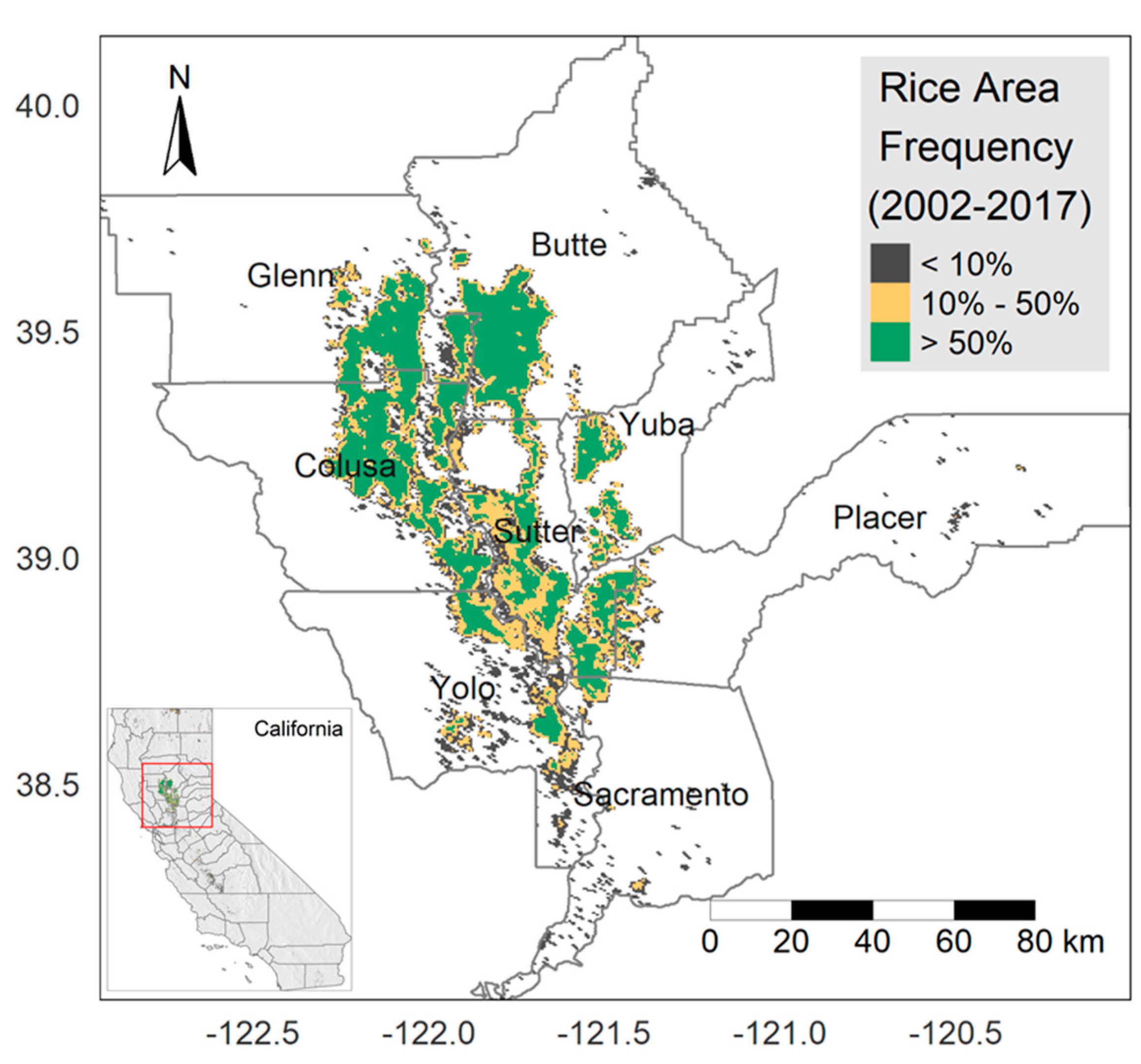
The yearly average area planted with rice in California is about 211,732 ha during 2000–2019 [49]. Over 95% of California’s rice production is in eight counties (Glenn, Butte, Colusa, Sutter, Yuba, Yolo, Sacramento and Placer) located in the Sacramento Valley (Figure 1). The average rice parcel size was 21 ha in 2014 (derived from CADWR [50]). All California rice is irrigated, and the growing season is characterized by a Mediterranean summer climate with dry hot days (31–35 °C) and cool nights (15–18 °C) [51,52]. Rice is direct seeded (primarily water seeded) on heavy clay soils in April or May and harvested in mid-September through October. The typical growing season length (from planting to harvest) is 140 to 145 days [53].
2.2. Estimation of Rice Area and Phenology Using Satellite Data
2.2.1. Satellite Data Processing
We used the 8-day Terra MODIS Surface Reflectance Product (MOD09A1) with a spatial resolution of 500 m for 2002–2017 [54]. The 8-day temporal resolution sets the accuracy at the pixel level, but not for the aggregated (e.g., county or state) level averages that we report. We used quality control flags to select cloud and shadow-free pixels over the land areas and then computed the EVI and NDFI as follows:
where ρ represents reflectance at different wavelengths: red (620–670 nm), near-infrared (nir, 841–876 nm), blue (459–479 nm) and shortwave-infrared (swir, 2105–2155 nm).
EVI = 2.5 × (ρnir − ρred)/(ρnir +6 × ρred −7.5 × ρblue + 1)
NDFI = (ρred − ρswir)/(ρred + ρswir)
We utilized the land surface daytime temperature (LST) from the MOD11A2 Terra MODIS product [55]. We first performed temporal gap-filling with cubic spline interpolation to fill in the cloud-contaminated or noisy pixels and applied the Savitzky–Golay filter iteratively to reconstruct the time series by fitting the upper envelope of the gap filled signal [56]. Finally, spatial resampling of these indices was performed to create consistent records of EVI, NDFI and LST at the 8-day temporal interval and 500 m spatial resolution. The entire analysis was conducted using the R Language and Environment for Statistical Computing with R version 3.6.2 [57].
2.2.2. Model Parameter Description and Calibration
We adapted the PhenoRice method [44,45] and adjusted the parameters to estimate the area planted to rice, the planting date, heading date and harvest date. From these dates the total growing season length, the duration of planting to heading (pre-heading period) and the growing length from heading to harvest (post-heading period) were computed.
In this study, planting date (the day that rice seed is broadcast on the flooded field) corresponds to the date with minimum EVI of the rice cycle signal; heading (the time when the panicle begins to exert from the boot) is as the date that EVI signal drops below a defined percentage (10%) of observed EVI range, and harvest date (the time when crop is gathered from the field) is as the date that EVI signal drops below a defined percentage (70%) of the observed EVI range. Most rice fields are planted with rice every year. Therefore, pixels that were only identified as rice once between 2002 and 2017 were considered erroneous outliers and removed (Figure 1).
We used PhenoRice as described in detail by Boschetti et al. [44] and Busetto et al. [45], with the following modifications: 1) parameters were changed to match local growing and management conditions and 2) for comparison with the field data, heading date was estimated instead of flowering date by using the date when EVI had decreased by 10% of the EVI range after the date of maximum EVI. Some parameters are slightly modified for California rice growing conditions with expert local knowledge, such as potential growing season length and flowering period. The description of each parameter and threshold used are provided in Table S1. An example of PhenoRice results for a pixel is also provided in Figure S1. Our implementation of PhenoRice algorithm is available as an R package [58].
2.3. Comparison of Satellite Data-Based Estimates with Reference Data
We compared our remote sensing data derived rice observations with data provided by the National Agricultural Statistics Service (NASS) of the United States Department of Agriculture (USDA) [59]. First, we compared the spatial distribution of rice between satellite estimates and Cropland Data Layer (CDL) [48] using the kappa statistic for the period of 2007–2017 as CDL data for California is not available prior to 2007. The CDL is an annual crop-specific categorized land cover product derived from medium resolution satellite data (Landsat 4/5/7/8, the Disaster Monitoring Constellation DEIMOS-1 and UK2, the ISRO ResourceSat 1 and 2, and the ESA SENTINEL-2 A and B), agricultural ground truth, and other ancillary data using a supervised decision tree classification with accuracy ranging from 85% to 95% [60]. For this comparison we created a binary “rice”–“no rice” class from CDL layers and aggregated these data from 30 m (for year 2008–2017) or 56 m (for year 2007) spatial resolution to 500 m using a majority rule (pixels with ≥ 50% rice occupancy labeled as rice). Second, we compared our rice area estimates with the USDA reported harvested area at county and state levels between 2002 and 2017 [49] using linear regression models. Third, we used linear regression to compare our estimated planting, heading and harvest dates at state level with USDA survey data for 2002–2017 [49]. The USDA provides state level estimates of crop phenology collected each week during the growing season [49]. These data include estimates of the percentage of the rice crop that had been planted, headed and harvested. These values were linearly interpolated to estimate the date when 50% of the rice crop reached a specific phenological stage. A linear regression analysis was then conducted between each satellite estimated growth stage date and its corresponding USDA reported date.
For the linear regression models, we computed p-values and R2 as well as the root mean square error (RMSE), relative RMSE (RMSE divided by the mean observed data) and mean absolute error (MAE) to quantify the performance of the satellite-based estimates [61].
2.4. Effect of Weather Variation on Phenological Information
We used our satellite-based estimates to study the effect of weather variation (precipitation and mean temperature) on rice phenology. Linear regression models were used to analyze the relationships between:
(i) Planting date and total precipitation from March (1 March) to April (30 April) (pre-season precipitation), as fields are usually drained to dry out the soils during February;
(ii) Planting date and average mean temperature from the middle of April (16 April) to the middle of May (15 May) (pre-season temperature), as the average planting date during the past decades was around the middle of May;
(iii–iv) Heading date (or pre-heading period length) and average mean temperature from the middle of May (16 May) to the middle of August (15 August) (pre-heading season temperature);
(v–vi) Harvesting date (or post-heading period length) and average mean temperature from the middle of August (16 August) to early October (10 October) (post-heading season temperature);
(vii) Total rice growing length and average mean temperatures from the middle of May (16 May) to early October (10 October) (the entire rice growing season).
We also analyzed temporal trends of phenology and weather data for each county and the whole state with linear regression using yearly averaged variables.
We used PRISM gridded precipitation and temperature data at 4-km spatial resolution from 2002 to 2017 [62]. Monthly precipitation and mean temperature data were used to calculate the average annual weather condition, including total precipitation and mean temperature for the rice region in California. The monthly precipitation data was also used to calculate the total precipitation before the rice growing season. Daily mean temperature data was used to calculate the average growing season mean temperate. We conducted the analysis between weather and rice phenology with rice area-weighted county and state-level averages.
2.5. Comparison of Satellite Predictions with Phenology Model
The timing of the heading determined with PhenoRice was also compared to predictions with the degree-day-10 (DD10) model developed for California rice [63]. This is a temperature-driven phenology model commonly used to predict rice developmental stages [17] and where a specified thermal time accumulation is required to complete any given growth stage. We used DD10 parameters by Sharifi et al. [63] for variety M-206 (the most widely grown variety in California during the study period (Figure S2)). The model was run with PRISM daily minimum and maximum temperature, and our satellite-based estimations of planting dates.
3. Results
3.1. Spatio-Temporal Distribution of Areas under Rice and Comparison with Official Statistics
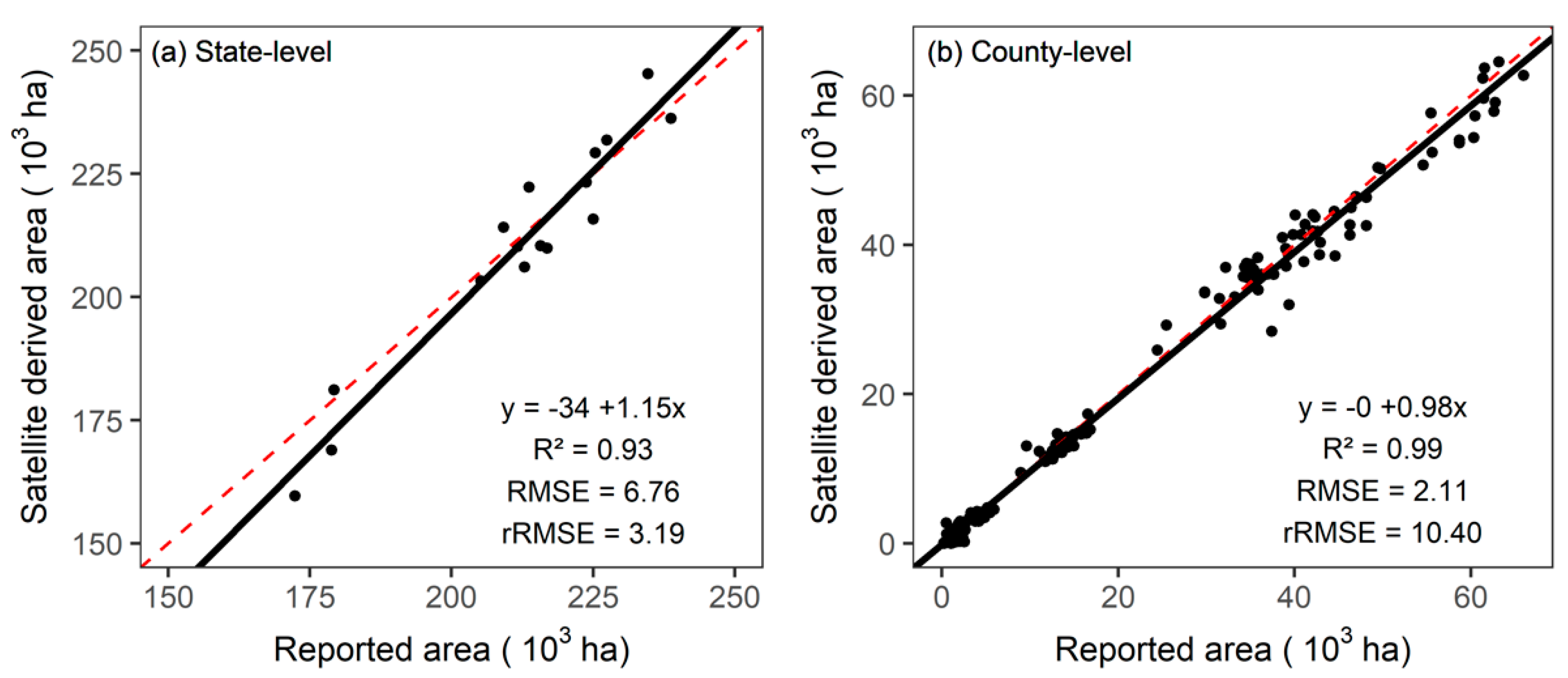
The satellite-based estimates of rice area in California are shown in Figure 1. At the state level, our estimates were very similar to the reported harvested area (USDA) for 2002–2017 (R2 = 0.93; p < 0.001) with an RMSE of 6762 ha, and a relative root mean square error (rRMSE) of 3.2% (Figure 2a and Table S2). There was also a strong linear relationship between our estimates and the reported county level rice area (USDA) (R2 = 0.99; p < 0.001) with an RMSE of 2108 ha and rRMSE of 10.4% (Figure 2b). When comparing county level data for each year separately, the R2 was above 0.95 for all cases, with an RMSE between 1194 and 4552 ha and the rRMSE between 5.6 and 17.3% (Table S2). The spatial agreements of our estimates with the Cropland Data Layer were also high with kappa coefficients between 0.85 and 0.91 for 2007 to 2017 (Table S2).
3.2. Rice Phenology Estimates
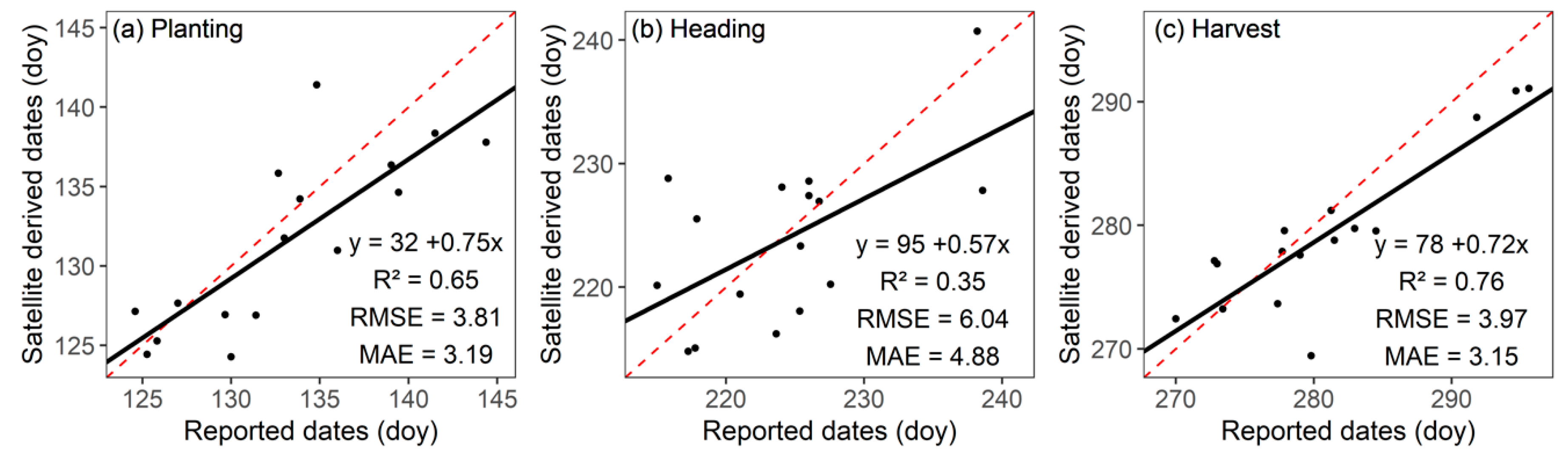
The quality of our satellite data-based phenology estimates varied with growth stages. The estimated planting dates show good agreement with the USDA reported dates during 2002–2017 (R2 = 0.65; p < 0.001; RMSE = 3.8 days; MAE = 3.2 days) (Figure 3a). However, the agreement is relatively poor for heading date (R2 = 0.35; p < 0.05; RMSE = 6.0 days; MAE = 4.9 days) (Figure 3b). The estimated harvest dates show strongest agreement (R2 = 0.76; p < 0.001; RMSE = 4.0 days; MAE = 3.2 days) (Figure 3c). Figure S3 provides a visual comparison of the satellite data-based estimates and USDA reported progress of planting, heading and harvest dates for each year. Satellite data-based estimates of heading dates were also correlated with heading dates predicted by the DD10 phenological model (R2 = 0.57; p < 0.001) with an RMSE of 4.4 days (Figure S4). There was no significant trend in planting, heading, and harvest dates, and lengths of pre-heading, post-heading and total rice growing season from 2002 to 2017 at the state level (Figure S5).
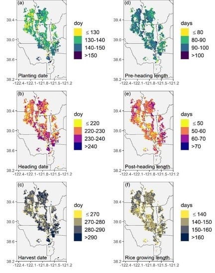
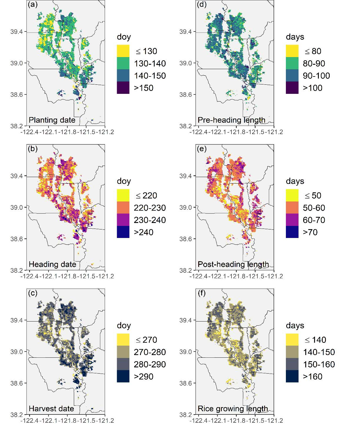
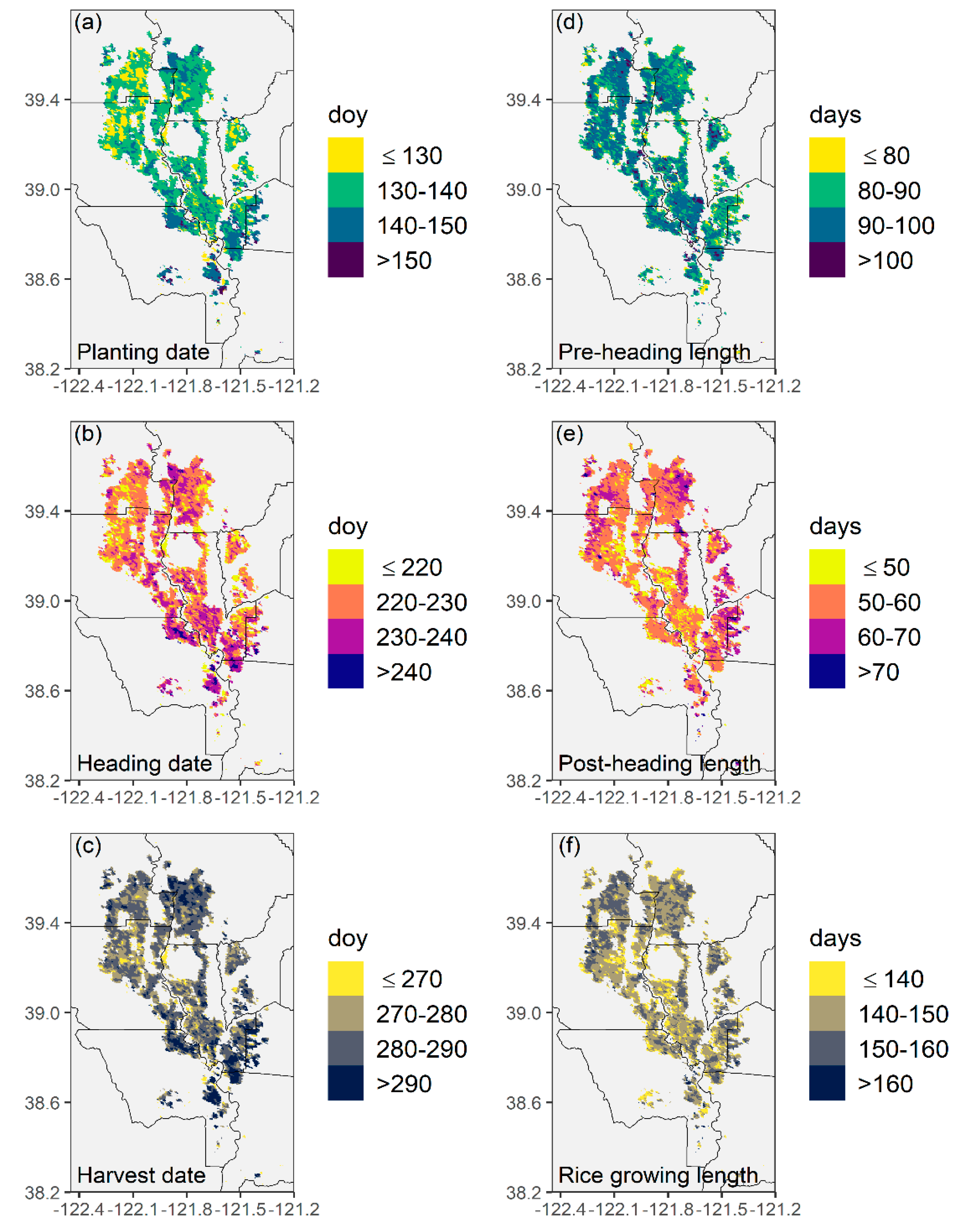
Our satellite data-based estimates showed that the growth stages and growing periods of rice varied temporally between years and spatially between counties (Figure S6). The spatial variation was most notable when contrasting the northern and southern part of the study region. Generally, it took longer to reach a given phenological stage in the southern than in the northern part of the region (Figure 4a–c). On average, in the southernmost rice growing counties (Sacramento, Yolo and Placer), rice was planted from 20 to 22 May (doy 140–142), headed from 16 to 21 August (doy 228–233) and harvested from 13 to 18 October (doy 286–291). In contrast, in the northern five counties, rice was planted from 13 to 17 May (doy 133–137), headed from 11 to 15 August (doy 223–227) and harvested from 7 to 12 October (doy 280–285). The length of the pre-heading season was 87–93 days (Figure 4d) and the post-heading period was 54–62 days for rice in California (Figure 4e). Placer county had the shortest pre-heading season length (87 days) and the longest post-heading season length (62 days), while in Sacramento county the situation was reversed, with 93 days pre-heading season and 54 days post-heading season. Thus, the average rice season was about 146–149 days and there were no clear differences in total season length between counties, although the northernmost rice growing counties had relatively long growing seasons, for example, 149 days in Glenn and 148 days in Butte (Figure 4f). There were no general trends in phenology over time (Table S3).
3.3. Phenology in Relation to Temperature and Precipitation
During the 2002–2017 study period, the average annual total precipitation in the rice areas was highest in Butte County (625 mm) and lowest in Sacramento County (423 mm) (Figure S7a). The average annual mean temperature was highest in Glenn county (17.1 °C) and lowest in Sacramento county (16.5 °C) (Figure S7b). There was a decreasing temperature gradient from the north to the south (the south is affected by cool weather coming in from the Pacific Ocean, a phenomenon referred to as the “Delta breeze”). From 2002 to 2017, there were no significant temperature and precipitation trends in most rice regions except warming in Glenn County (Table S4).
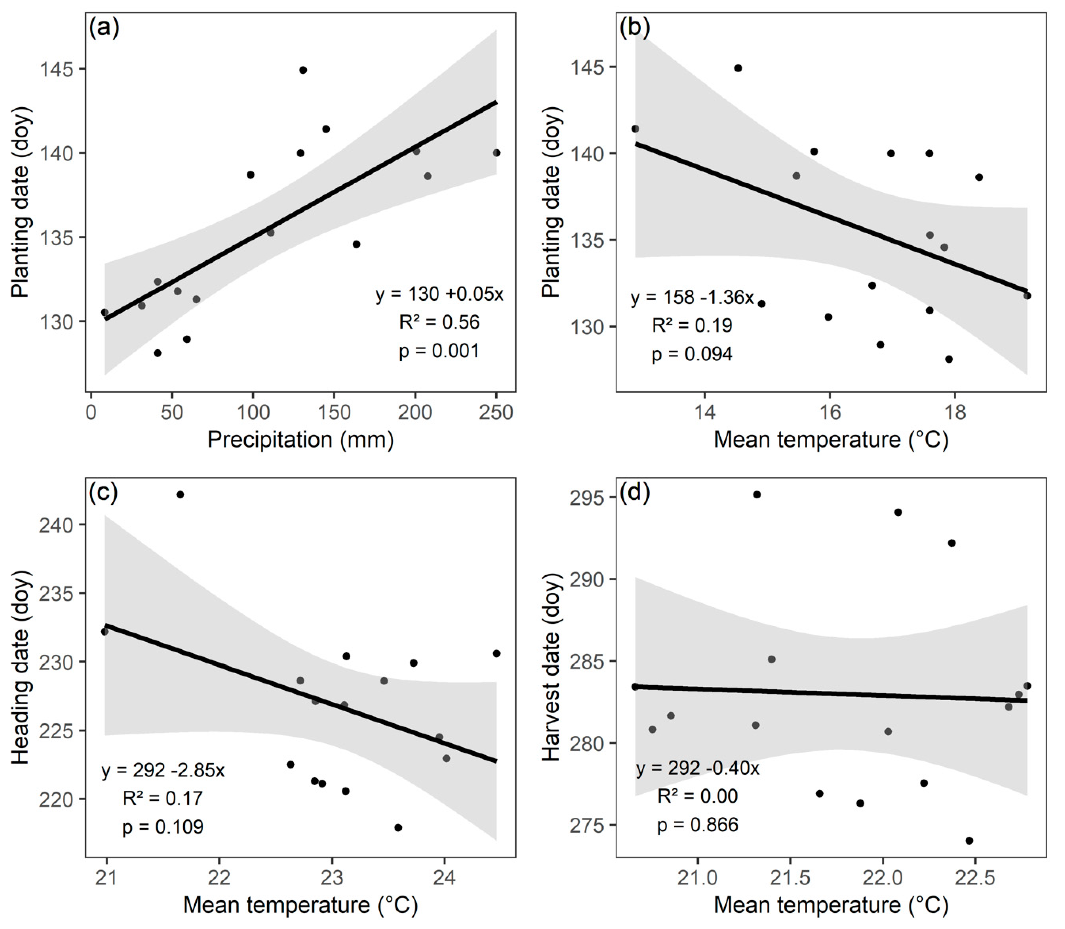
We found that the rice planting date estimated with satellite data was significantly delayed by 5.3 days for every 100 mm increase in total precipitation during March and April (p = 0.001) (Figure 5a), while it was advanced by 1.4 days for every 1°C increase in mean temperature before planting (mid-April to mid-May) (p = 0.09) (Figure 5b). Increased temperature during the pre-heading period advanced the heading date by 2.9 days °C−1, but this relation only had weak statistical support (p = 0.11) (Figure 5c). The DD10 model predicted a 3.4-day earlier heading date for 1 °C increase of mean temperature during the pre-heading period (Figure S8a). There was no effect of mean temperature during the post-heading period on harvest date (Figure 5d).
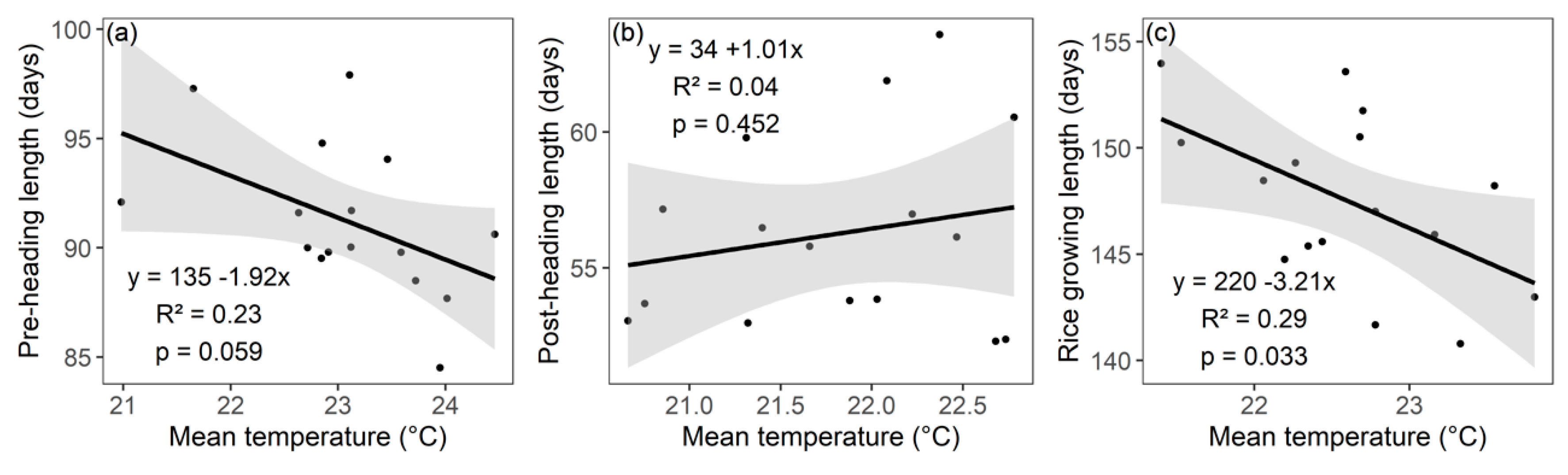
At the state level, the total rice growing season length and pre-heading growth duration were negatively correlated with mean temperature (Figure 6). An increase in the average pre-heading season temperature of 1 °C was associated with a 1.9-day shorter pre-heading duration (Figure 6a). The DD10 model showed a slightly stronger trend with a decrease in pre-heading length of 2.4 days for each 1 °C increase in mean temperature (Figure S8b). While there was no obvious effect of temperature on the post-heading growing season length (Figure 6b), total growing season length was reduced by 3.2 days °C -1 (Figure 6c).
At the county level, rice planting dates were earlier under warm conditions, while they were later under wet conditions of the pre-season during the study period (Table 1). Rice planting was earlier by 0.7–2.3 days °C−1 (mean temperature of the pre-season), while planting was delayed by 4.1–6.3 days for each 100 mm precipitation increase in the pre-season. Heading dates advanced by 1.8–3.9 days °C−1 during the pre-heading season and the duration from planting to heading was shortened by 1.1–3.1 days °C−1. The total season length was shortened by 2.3–4.2 days °C−1, and this effect was particularly pronounced in Butte and Glenn counties. There were no temperature effects on the length of the post-heading period or on harvest date.
4. Discussion
We used time-series satellite data and a rule-based model (PhenoRice) to estimate the area planted to rice and its key growth stages in California. Our estimates were similar to the numbers reported by the USDA and the spatial patterns of rice growing areas had good agreement with existing crop distribution data (Cropland Data Layer). These results suggest that PhenoRice can be used for identifying rice in regions like California with relatively large and homogenous fields, and a single rice growing season. The performance of PhenoRice for detecting rice area in this study was similar to or better than previous applications of PhenoRice in other regions of the world [44,45] and also to other MODIS-based studies on rice mapping in different regions [32,64,65,66].
There are two important factors that may explain the satisfactory performance of PhenoRice in California. First, the average parcel size of rice in California is large compared to other rice growing areas across the world. The average parcel size was 21 ha in 2014 [50]. This dimension is roughly equal to the size of a MODIS pixel (25 ha), likely leading to a relatively low within-pixel heterogeneity. Second, the number of cloud-free satellite observations during the summer rice growing season in California is much higher than in many other rice growing areas where production primarily takes place during the rainy season, resulting in a reliable representation of rice growth by EVI and NDFI. In this study, we used MODIS because of the availability of a long-term time series. Future studies could investigate the use of higher spatial resolution optical data from Landsat and Sentinel 2, as well as Sentinel 1 data (radar).
We found good agreements for planting and harvesting dates with the reported data, but not for heading. Smoothed EVI signal can’t capture all the detailed and subtle changes around the peak of the growing season and may fail to accurately detect the heading events. In this study, the field observations of phenology were only available at the state level. The evaluation of the estimation could be improved by collecting observations at specific locations. The accuracy of detecting rice planting and harvest dates in our study is similar to results obtained by others with PhenoRice. Boschetti et al. [44] found a MAE of 10.0 days between the PhenoRice establishment dates in Italy, India and the Philippines and the reference data. Busetto et al. [45] found an RMSE of 5.4–8.2 days for establishment and harvesting dates in Senegal. Overall, our results suggest that key growth dates can be reliably estimated from satellite data with PhenoRice.
In contrast to these prior PhenoRice studies, we also compared estimated heading dates with the reported data and with a temperature-driven phenology model. These results were better than earlier work using other methods. For example, Sakamoto et al. [41] reported an RMSE of 9–12.1 days in the estimation of phenological dates (including planting, heading and harvesting dates) in Japan. Li et al. [40] reported an RMSE around 10 days in the estimation of transplanting, tillering, heading, and harvesting dates in Jiangsu, China. PhenoRice also shows improved applicability across different rice environments (regionally and temporally) [44,45,46,47] when compared with other methods [67,68,69]. However, the model requires user-specified input parameters that depend on the local rice growing conditions. These parameters may vary with cropping practices, particularly in larger regions with multiple agro-climatic conditions, and perhaps multiple crops per year.
We found that planting occurred earlier in the warmer conditions, and later in wetter conditions because famers do not plant rice when it is too cold, or when the conditions are too wet for seedbed preparation [70]. The results also suggest that increased growing season temperatures can advance the phenological dates and reduce crop growth duration. Between 2002 and 2017, there was no clear trend in temperatures or rainfall in the rice growing regions of California and thus the effects of climate change could not be examined. Nevertheless, our results on variability in rice phenology due to weather variation could be useful for understanding climate change effects. The responses we found were in agreement with climate change responses reported by others. For example, Ye et al. [71] reported that the rice growing season length was reduced by 3.1 days per 1 ℃ increase temperature in a single rice system in China. Zhang et al. [72] reported that growth duration length could be shortened by 3.0 days ℃−1 from emergence to heading, and 1.1 days ℃−1 from heading to maturity and 4.4 days ℃−1 from emergence to maturity. Earlier transplanting and heading dates were found to be related to the increased mean air temperature in Japan [73]. We found it reassuring that, despite the uncertainty in the satellite phenology data, we were able to detect crop responses that made sense from a farm management and a crop physiology perspective.
The DD10 model predicted similar but stronger effects of temperature on phenology than our PhenoRice estimates. This may be partly due to changes in varieties over time. For the DD10 model estimation, we used M-206, the main variety grown in California during the study period. Other varieties with different phenology characteristics are also grown by the farmers (Figure S2). For example, prior to 2005, M-202 was the main rice variety and it reached heading about 4–5 days later that M-206. The weaker effects of temperature on phenology predicted with satellite observation maybe thus in part be due to farmer behaviors, that is, adjusting varieties grown suitable for the changing conditions.
In the southern part of our study area, shorter duration varieties like M-206 are grown to a greater extent than in the northern counties where longer duration varieties do better. We observed a longer growing season in these warmer parts of the study region, providing empirical evidence that farmers adopt the varieties to make best use of the growing season that is available to them. While the satellite data do not differentiate between varieties, it does have the ability to capture the difference in crop responses to weather conditions. These findings suggest that remote sensing can be used to detect the crop phenology and may be more useful than weather-driven phenology models to study the variation in crop phenology.
5. Conclusions
In this study, we mapped rice phenology in California over 16 years using satellite data and we analyzed the relation between the observed phenology and weather. We found that the satellite-based estimates of rice area correspond well with field surveys and other data provided by the USDA. Satellite-based estimates of planting and harvesting date were more accurate than estimates of heading date. This study suggests that crop phenology derived from remote sensing data can be used to monitor agriculture systems and supplement ground observations. The satellite data derived phenology allowed for a more refined understanding of how rice farming responds to variation in weather conditions. These insights can be used to understand the different management strategies and possibly for climate change adaptations, to make crop model based studies more realistic, and to improve projections of agricultural responses to weather variability and climate change as well.
Supplementary Materials
The following are available online at https://www.mdpi.com/2072-4292/12/9/1522/s1, Figure S1: Example of PhenoRice results for a rice pixel in California, Figure S2: Medium grain variety acreage as a percent of total medium grain acreage from 2000 to 2019. (During this period medium grains averaged 90% (range 86%–94%) of total acreage in CA based on the Quick Stats Database published by USDA NASS), Figure S3: Estimated and reported (a) planting, (b) heading and (c) harvest dates occurred at California State by percent area, Figure S4: Comparison between satellite derived and DD10 simulated heading dates in California from 2002 to 2017, Figure S5: Estimated (a) planting, (b) heading and (c) harvest dates, (d) growing period from planting to heading, (e) heading to harvest and (f) planting to harvest for California at state level from 2002 to 2017, Figure S6: Spatial maps of (a) planting dates, (b) heading date, (c) harvest date, (d) growing length from planting to heading, (e) growing length from heading to harvest, (f) total growing length from planting to harvest during 2002–2017 in Sacramento Valley, Figure S7: Average (a) annual total precipitation and (b) mean temperature of rice regions in Sacramento Valley during 2002–2017, Figure S8: The relationships (a) between average mean temperature of pre-heading season and simulated heading dates; (b) between the pre-heading season mean temperature and growing length from planting to heading for rice region in California, Table S1: PhenoRice parameters used for analysis, Table S2: California state-level satellite estimated rice area and USDA surveyed rice area, and the slope (p < 0.001 for all slopes), R2, RMSE and rRMSE of the linear regression between California county-level satellite estimated rice area and USDA survey or census reported (in parenthesis) rice area for 2002–2017, and kappa coefficients between satellite detected rice area and CDL identified rice area for 2007–2017, Table S3: Annual trends of estimated planting, heading and harvest dates, growing periods from planting to heading (vlength), heading to harvest (rlength) and planting to harvest (tlength) for California at county level from 2002 to 2017 (p < 0.01 **, p < 0.05 *), Table S4: Annual trends of total precipitation and average mean temperature for California at county level from 2002 to 2017 (p < 0.05 *).
Author Contributions
Conceptualization, H.W.; methodology, H.W., A.G. and R.J.H.; formal analysis, H.W; supervision, H.W. and R.J.H.; writing–original draft preparation, H.W. and R.J.H.; writing–review and editing, H.W., R.J.H., B.A.L. and A.G. All authors have read and agreed to the published version of the manuscript.
Funding
This research received no external funding.
Conflicts of Interest
The authors declare no conflicts of interest.
References
- Chmielewski, F.-M.; Müller, A.; Bruns, E. Climate changes and trends in phenology of fruit trees and field crops in Germany, 1961–2000. Agric. For. Meteorol. 2004, 121, 69–78. [Google Scholar] [CrossRef]
- Hatfield, J.L.; Prueger, J.H. Temperature extremes: Effect on plant growth and development. Weather Clim. Extrem. 2015, 10, 4–10. [Google Scholar] [CrossRef] [Green Version]
- Liu, Y.; Chen, Q.; Ge, Q.; Dai, J.; Qin, Y.; Dai, L.; Zou, X.; Chen, J. Modelling the impacts of climate change and crop management on phenological trends of spring and winter wheat in China. Agric. For. Meteorol. 2018, 248, 518–526. [Google Scholar] [CrossRef]
- Anwar, M.R.; Liu, D.L.; Farquharson, R.J.; Macadam, I.; Abadi, A.; Finlayson, J.; Wang, B.; Ramilan, T. Climate change impacts on phenology and yields of five broadacre crops at four climatologically distinct locations in Australia. Agric. Syst. 2015, 132, 133–144. [Google Scholar] [CrossRef] [Green Version]
- Brown, M.E.; De Beurs, K.M.; Marshall, M. Global phenological response to climate change in crop areas using satellite remote sensing of vegetation, humidity and temperature over 26years. Remote Sens. Environ. 2012, 126, 174–183. [Google Scholar] [CrossRef]
- Sacks, W.J.; Kucharik, C.J. Crop management and phenology trends in the U.S. Corn Belt: Impacts on yields, evapotranspiration and energy balance. Agric. For. Meteorol. 2011, 151, 882–894. [Google Scholar] [CrossRef]
- Barlow, K.; Christy, B.; O’Leary, G.; Riffkin, P.; Nuttall, J. Simulating the impact of extreme heat and frost events on wheat crop production: A review. Field Crop. Res. 2015, 171, 109–119. [Google Scholar] [CrossRef] [Green Version]
- Challinor, A.J.; Wheeler, T.; Craufurd, P.; Slingo, J. Simulation of the impact of high temperature stress on annual crop yields. Agric. For. Meteorol. 2005, 135, 180–189. [Google Scholar] [CrossRef] [Green Version]
- Fitchett, J.M.; Grab, S.; Thompson, D.I. Plant phenology and climate change. Prog. Phys. Geogr. Earth Environ. 2015, 39, 460–482. [Google Scholar] [CrossRef]
- Tao, F.; Yokozawa, M.; Xu, Y.; Hayashi, Y.; Zhang, Z. Climate changes and trends in phenology and yields of field crops in China, 1981–2000. Agric. For. Meteorol. 2006, 138, 82–92. [Google Scholar] [CrossRef]
- Cleland, E.E.; Chuine, I.; Menzel, A.; Mooney, H.A.; Schwartz, M. Shifting plant phenology in response to global change. Trends Ecol. Evol. 2007, 22, 357–365. [Google Scholar] [CrossRef] [PubMed]
- Menzel, A.; von Vopelius, J.; Estrella, N.; Schleip, C.; Dose, V. Farmers’ annual activities are not tracking the speed of climate change. Clim. Res. 2006, 32, 201–207. [Google Scholar]
- Wang, J.; Wang, E.; Feng, L.; Yin, H.; Yu, W. Phenological trends of winter wheat in response to varietal and temperature changes in the North China Plain. Field Crop. Res. 2013, 144, 135–144. [Google Scholar] [CrossRef]
- Oteros, J.; Garcia-Mozo, H.; Botey, R.; Mestre, A.; Galán, C. Variations in cereal crop phenology in Spain over the last twenty-six years (1986–2012). Clim. Chang. 2015, 130, 545–558. [Google Scholar] [CrossRef]
- Rezaei, E.E.; Siebert, S.; Hüging, H.; Ewert, F. Climate change effect on wheat phenology depends on cultivar change. Sci. Rep. 2018, 8, 4891. [Google Scholar] [CrossRef] [Green Version]
- Hussain, J.; Khaliq, T.; Ahmad, A.; Akhtar, J. Performance of four crop model for simulations of wheat phenology, leaf growth, biomass and yield across planting dates. PLoS ONE 2018, 13, e0197546. [Google Scholar] [CrossRef]
- Counce, P.A.; Siebenmorgen, T.J.; Ambardekar, A.A. Rice reproductive development stage thermal time and calendar day intervals for six US rice cultivars in the Grand Prairie, Arkansas, over 4 years. Ann. Appl. Boil. 2015, 167, 262–276. [Google Scholar] [CrossRef]
- Sharifi, H.; Hijmans, R.J.; Hill, J.E.; Linquist, B.A. Using Stage-Dependent Temperature Parameters to Improve Phenological Model Prediction Accuracy in Rice Models. Crop. Sci. 2016, 57, 444–453. [Google Scholar] [CrossRef] [Green Version]
- Keating, B.; Carberry, P.; Hammer, G.L.; Probert, M.; Robertson, M.; Holzworth, D.; Huth, N.; Hargreaves, J.; Meinke, H.; Hochman, Z.; et al. An overview of APSIM, a model designed for farming systems simulation. Eur. J. Agron. 2003, 18, 267–288. [Google Scholar] [CrossRef] [Green Version]
- Bouman, B.; Van Laar, H. Description and evaluation of the rice growth model ORYZA2000 under nitrogen-limited conditions. Agric. Syst. 2006, 87, 249–273. [Google Scholar] [CrossRef]
- Wallach, D.; Palosuo, T.; Thorburn, P.; Seidel, S.J.; Gourdain, E.; Asseng, S.; Basso, B.; Buis, S.; Crout, N.M.J.; Dibari, C.; et al. How well do crop models predict phenology, with emphasis on the effect of calibration? BioRxiv 2019, 708578. [Google Scholar] [CrossRef] [Green Version]
- Asseng, S.; Ewert, F.; Martre, P.; Rotter, R.; Lobell, D.B.; Cammarano, D.; Kimball, B.A.; Ottman, M.J.; Wall, G.W.; White, J.W.; et al. Rising temperatures reduce global wheat production. Nat. Clim. Chang. 2014, 5, 143–147. [Google Scholar] [CrossRef]
- Chen, Y.; Zhang, Z.; Tao, F.; Palosuo, T.; Rotter, R.; Rötter, R.P. Impacts of heat stress on leaf area index and growth duration of winter wheat in the North China Plain. Field Crop. Res. 2018, 222, 230–237. [Google Scholar] [CrossRef] [Green Version]
- Lobell, D.B.; Sibley, A.; Ortiz-Monasterio, J.I. Extreme heat effects on wheat senescence in India. Nat. Clim. Chang. 2012, 2, 186–189. [Google Scholar] [CrossRef]
- Zhang, S.; Tao, F. Modeling the response of rice phenology to climate change and variability in different climatic zones: Comparisons of five models. Eur. J. Agron. 2013, 45, 165–176. [Google Scholar] [CrossRef]
- Lobell, D.B.; Ortiz-Monasterio, J.I.; Sibley, A.M.; Sohu, V. Satellite detection of earlier wheat sowing in India and implications for yield trends. Agric. Syst. 2013, 115, 137–143. [Google Scholar] [CrossRef]
- Piao, S.; Fang, J.; Zhou, L.; Ciais, P.; Zhu, B. Variations in satellite-derived phenology in China’s temperate vegetation. Glob. Chang. Biol. 2006, 12, 672–685. [Google Scholar] [CrossRef]
- Piao, S.; Liu, Q.; Chen, A.; Janssens, I.A.; Fu, Y.H.; Dai, J.; Liu, L.; Lian, X.; Shen, M.; Zhu, X. Plant phenology and global climate change: Current progresses and challenges. Glob. Chang. Boil. 2019, 25, 1922–1940. [Google Scholar] [CrossRef]
- Whitcraft, A.K.; Becker-Reshef, I.; Killough, B.; Justice, C. Meeting Earth Observation Requirements for Global Agricultural Monitoring: An Evaluation of the Revisit Capabilities of Current and Planned Moderate Resolution Optical Earth Observing Missions. Remote. Sens. 2015, 7, 1482–1503. [Google Scholar] [CrossRef] [Green Version]
- Pan, Y.; Li, L.; Zhang, J.; Liang, S.; Zhu, X.; Sulla-Menashe, D. Winter wheat area estimation from MODIS-EVI time series data using the Crop Proportion Phenology Index. Remote Sens. Environ. 2012, 119, 232–242. [Google Scholar] [CrossRef]
- Wardlow, B.D.; Egbert, S.L. Large-area crop mapping using time-series MODIS 250 m NDVI data: An assessment for the U.S. Central Great Plains. Remote Sens. Environ. 2008, 112, 1096–1116. [Google Scholar] [CrossRef]
- Xiao, X.; Boles, S.; Liu, J.; Zhuang, D.; Frolking, S.; Li, C.; Salas, W.; Moore, B. Mapping paddy rice agriculture in southern China using multi-temporal MODIS images. Remote Sens. Environ. 2005, 95, 480–492. [Google Scholar] [CrossRef]
- Biradar, C.; Xiao, X. Quantifying the area and spatial distribution of double- and triple-cropping croplands in India with multi-temporal MODIS imagery in 2005. Int. J. Remote Sens. 2011, 32, 367–386. [Google Scholar] [CrossRef]
- Frolking, S.; Qiu, J.; Boles, S.; Xiao, X.; Liu, J.; Zhuang, Y.; Li, C.; Qin, X. Combining remote sensing and ground census data to develop new maps of the distribution of rice agriculture in China. Glob. Biogeochem. Cycles 2002, 16, 38–41. [Google Scholar] [CrossRef] [Green Version]
- Li, L.; Friedl, M.; Xin, Q.; Gray, J.; Pan, Y.; Frolking, S. Mapping Crop Cycles in China Using MODIS-EVI Time Series. Remote Sens. 2014, 6, 2473–2493. [Google Scholar] [CrossRef] [Green Version]
- Boschetti, M.; Stroppiana, D.; Brivio, P.A.; Bocchi, S. Multi-year monitoring of rice crop phenology through time series analysis of MODIS images. Int. J. Remote. Sens. 2009, 30, 4643–4662. [Google Scholar] [CrossRef]
- Lu, L.; Wang, C.; Guo, H.; Li, Q. Detecting winter wheat phenology with SPOT-VEGETATION data in the North China Plain. Geocarto Int. 2013, 29, 244–255. [Google Scholar] [CrossRef]
- Sakamoto, T.; Wardlow, B.D.; A Gitelson, A.; Verma, S.; Suyker, A.E.; Arkebauer, T.J. A Two-Step Filtering approach for detecting maize and soybean phenology with time-series MODIS data. Remote. Sens. Environ. 2010, 114, 2146–2159. [Google Scholar] [CrossRef]
- You, X.; Meng, J.; Zhang, M.; Dong, T. Remote Sensing Based Detection of Crop Phenology for Agricultural Zones in China Using a New Threshold Method. Remote. Sens. 2013, 5, 3190–3211. [Google Scholar] [CrossRef] [Green Version]
- Li, S.; Xiao, J.; Ni, P.; Zhang, J.; Wang, H.S.; Wang, J.X. Monitoring paddy rice phenology using time series MODIS data over Jiangxi Province, China. Int. J. Agric. Biol. Eng. 2014, 7, 28–36. [Google Scholar]
- Sakamoto, T.; Yokozawa, M.; Toritani, H.; Shibayama, M.; Ishitsuka, N.; Ohno, H. A crop phenology detection method using time-series MODIS data. Remote Sens. Environ. 2005, 96, 366–374. [Google Scholar] [CrossRef]
- Dash, J.; Jeganathan, C.; Atkinson, P. The use of MERIS Terrestrial Chlorophyll Index to study spatio-temporal variation in vegetation phenology over India. Remote Sens. Environ. 2010, 114, 1388–1402. [Google Scholar] [CrossRef]
- Kang, W.; Wang, T.; Liu, S. The Response of Vegetation Phenology and Productivity to Drought in Semi-Arid Regions of Northern China. Remote Sens. 2018, 10, 727. [Google Scholar] [CrossRef] [Green Version]
- Boschetti, M.; Busetto, L.; Manfron, G.; Laborte, A.; Asilo, S.; Pazhanivelan, S.; Nelson, A. PhenoRice: A method for automatic extraction of spatio-temporal information on rice crops using satellite data time series. Remote Sens. Environ. 2017, 194, 347–365. [Google Scholar] [CrossRef] [Green Version]
- Busetto, L.; Zwart, S.; Boschetti, M. Analysing spatial–temporal changes in rice cultivation practices in the Senegal River Valley using MODIS time-series and the PhenoRice algorithm. Int. J. Appl. Earth Obs. Geoinf. 2019, 75, 15–28. [Google Scholar] [CrossRef]
- Pagani, V.; Guarneri, T.; Busetto, L.; Ranghetti, L.; Boschetti, M.; Movedi, E.; Campos-Taberner, M.; García-Haro, F.J.; Katsantonis, D.; Stavrakoudis, D.; et al. A high-resolution, integrated system for rice yield forecasting at district level. Agric. Syst. 2019, 168, 181–190. [Google Scholar] [CrossRef]
- Setiyono, T.; Quicho, E.D.; Gatti, L.; Campos-Taberner, M.; Busetto, L.; Collivignarelli, F.; García-Haro, F.J.; Boschetti, M.; Khan, N.I.; Holecz, F. Spatial Rice Yield Estimation Based on MODIS and Sentinel-1 SAR Data and ORYZA Crop Growth Model. Remote Sens. 2018, 10, 293. [Google Scholar] [CrossRef] [Green Version]
- USDA National Agricultural Statistics Service Cropland Data Layer. Available online: https://nassgeodata.gmu.edu/CropScape/ (accessed on 29 April 2019).
- Quick Stats. United States Department of Agriculture National Agriculture and Statistics Service, Washington, DC, 2019. Available online: https://quickstats.nass.usda.gov/ (accessed on 18 March 2020).
- Crop Mapping 2014, California Department of Water Resources. Available online: https://data.cnra.ca.gov/dataset/crop-mapping-2014 (accessed on 15 April 2019).
- Brodt, S.; Kendall, A.; Mohammadi, Y.; Arslan, A.; Yuan, J.; Lee, I.-S.; Linquist, B.; Arslan, A. Life cycle greenhouse gas emissions in California rice production. Field Crop. Res. 2014, 169, 89–98. [Google Scholar] [CrossRef]
- Roel, A.; Plant, R.E.; Young, J.A.; Pettygrove, G.S.; Deng, J.; Williams, J.F. Interpreting yield patterns for California rice precision farm management. Proceedings of Fifth International Conference on Precision Agriculture (CD), Bloomington, MN, USA, 16–19 July 2000. [Google Scholar]
- Hill, J.E.; Williams, J.F.; Mutters, R.G.; Greer, C.A. The California rice cropping system: Agronomic and natural resource issues for long-term sustainability. Paddy Water Environ. 2006, 4, 13–19. [Google Scholar] [CrossRef]
- Vermote, E. MOD09A1 MODIS/Terra Surface Reflectance 8-Day L3 Global 500m SIN Grid V006. NASA EOSDIS Land Processes DAAC, 2015. Available online: https://doi.org/10.5067/MODIS/MOD09A1.006 (accessed on 2 May 2020).
- Wan, Z.; Hook, S.; Hulley, G. MOD11A2 MODIS/Terra Land Surface Temperature/Emissivity 8-Day L3 Global 1km SIN Grid V006. NASA EOSDIS Land Processes DAAC, 2015. Available online: https://doi.org/10.5067/MODIS/MOD11A2.006 (accessed on 2 May 2020).
- Chen, J.; Jönsson, P.; Tamura, M.; Gu, Z.; Matsushita, B.; Eklundh, L. A simple method for reconstructing a high-quality NDVI time-series data set based on the Savitzky–Golay filter. Remote Sens. Environ. 2004, 91, 332–344. [Google Scholar] [CrossRef]
- R Core Team. R: A Language and Environment for Statistical Computing; R Foundation for Statistical Computing: Vienna, Austria, 2019. Available online: https://www.R-project.org/ (accessed on 30 October 2019).
- Wang, H.; Ghosh, A.; Hijmans, R.J. Phenorice: An Implementation of Phenorice Algorithm to Detect Rice Crops from Remote Sensing Data. R Package Version: 0.1-1. 2019. Available online: https://github.com/cropmodels/phenorice (accessed on 20 February 2020).
- United States Department of Agriculture National Agricultural Statistics Service. Available online: http://www.nass.usda.gov/ (accessed on 3 May 2013).
- United States Department of Agriculture National Agricultural Statistics Service. Research and Science. Available online: https://www.nass.usda.gov/Research_and_Science/Cropland/sarsfaqs2.php (accessed on 3 May 2020).
- Montgomery, D.C.; Peck, E.A. Introduction to Linear Regression Analysis, 2nd ed.; Wiley: New York, NY, USA, 1992. [Google Scholar]
- PRISM Climate Group, Oregon State University. Available online: http://www.prism.oregonstate.edu/ (accessed on 14 May 2019).
- Sharifi, H.; Hijmans, R.J.; Hill, J.E.; Linquist, B. Water and air temperature impacts on rice (Oryza sativa) phenology. Paddy Water Environ. 2018, 16, 467–476. [Google Scholar] [CrossRef]
- Son, N.; Chen, C.; Chen, C.; Duc, H.; Chang, L. A Phenology-Based Classification of Time-Series MODIS Data for Rice Crop Monitoring in Mekong Delta, Vietnam. Remote Sens. 2013, 6, 135–156. [Google Scholar] [CrossRef] [Green Version]
- Sun, H.; Huang, J.; Huete, A.; Peng, D.; Zhang, F. Mapping paddy rice with multi-date moderate-resolution imaging spectroradiometer (MODIS) data in China. J. Zhejiang Univ. A 2009, 10, 1509–1522. [Google Scholar] [CrossRef]
- Zhang, G.; Xiao, X.; Dong, J.; Kou, W.; Jin, C.; Qin, Y.; Zhou, Y.; Wang, J.; Menarguez, M.A.; Biradar, C. Mapping paddy rice planting areas through time series analysis of MODIS land surface temperature and vegetation index data. ISPRS J. Photogramm. Remote Sens. 2015, 106, 157–171. [Google Scholar] [CrossRef] [PubMed] [Green Version]
- Kucuk, C.; Taskin, G.; Erten, E.; Taskın, G. Paddy-Rice Phenology Classification Based on Machine-Learning Methods Using Multitemporal Co-Polar X-Band SAR Images. IEEE J. Sel. Top. Appl. Earth Obs. Remote Sens. 2016, 9, 2509–2519. [Google Scholar] [CrossRef]
- Lopez-Sanchez, J.M.; Cloude, S.R.; Ballester-Berman, J.D. Rice Phenology Monitoring by Means of SAR Polarimetry at X-Band. IEEE Trans. Geosci. Remote Sens. 2012, 50, 2695–2709. [Google Scholar] [CrossRef]
- Wang, J.; Huang, J.; Wang, X.-Z.; Jin, M.-T.; Zhou, Z.; Guo, Q.-Y.; Zhao, Z.-W.; Huang, W.-J.; Zhang, Y.; Song, X.-D. Estimation of rice phenology date using integrated HJ-1 CCD and Landsat-8 OLI vegetation indices time-series images. J. Zhejiang Univ. Sci. B 2015, 16, 832–844. [Google Scholar] [CrossRef]
- Linquist, B.A.; Espe, M.B. When is the Optimal Time to Plant Rice in the Sacramento Valley? 2015. Available online: http://rice.ucanr.edu/files/232444.pdf (accessed on 1 November 2019).
- Ye, T.; Zong, S.; Kleidon, A.; Yuan, W.; Wang, Y.; Shi, P. Impacts of climate warming, cultivar shifts, and phenological dates on rice growth period length in China after correction for seasonal shift effects. Clim. Chang. 2019, 155, 127–143. [Google Scholar] [CrossRef] [Green Version]
- Zhang, T.; Huang, Y.; Yang, X. Climate warming over the past three decades has shortened rice growth duration in China and cultivar shifts have further accelerated the process for late rice. Glob. Chang. Boil. 2012, 19, 563–570. [Google Scholar] [CrossRef]
- Nguyen-Sy, T.; Cheng, W.; Tawaraya, K.; Sugawara, K.; Kobayashi, K. Impacts of climatic and varietal changes on phenology and yield components in rice production in Shonai region of Yamagata Prefecture, Northeast Japan for 36 years. Plant Prod. Sci. 2019, 22, 382–394. [Google Scholar] [CrossRef] [Green Version]
Figure 1.
Proportion of years with rice cultivation detected with the satellite data-based estimate for counties with most rice producing areas in California between 2002 and 2017.
Figure 1.
Proportion of years with rice cultivation detected with the satellite data-based estimate for counties with most rice producing areas in California between 2002 and 2017.

Figure 2.
Satellite data-based estimate of rice area versus the area reported by the United States Department of Agriculture for California from 2002 to 2017 at the (a) state level and (b) county level. Each dot represents a year. Black lines are regression lines and red dashed lines are y = x.
Figure 2.
Satellite data-based estimate of rice area versus the area reported by the United States Department of Agriculture for California from 2002 to 2017 at the (a) state level and (b) county level. Each dot represents a year. Black lines are regression lines and red dashed lines are y = x.

Figure 3.
Satellite-data based estimates versus USDA reported (a) planting, (b) heading, and (c) harvest time expressed as day of year (doy; the number of days since 31 December of the previous year) for rice in California. Black lines are regression lines, and red dashed lines are y = x.
Figure 3.
Satellite-data based estimates versus USDA reported (a) planting, (b) heading, and (c) harvest time expressed as day of year (doy; the number of days since 31 December of the previous year) for rice in California. Black lines are regression lines, and red dashed lines are y = x.

Figure 4.
Average (a) planting, (b) heading and (c) harvest dates, growing length of (d) pre-heading period, (e) post-heading period and (f) whole growing season of rice in the Sacramento Valley of California estimated with MODIS data and PhenoRice between 2002 and 2017.
Figure 4.
Average (a) planting, (b) heading and (c) harvest dates, growing length of (d) pre-heading period, (e) post-heading period and (f) whole growing season of rice in the Sacramento Valley of California estimated with MODIS data and PhenoRice between 2002 and 2017.

Figure 5.
The relationship between (a) satellite-observed planting date and the pre-season precipitation, (b) satellite-observed planting date and the average mean temperature of pre-season, (c) satellite-observed heading date and the average mean temperature of pre-heading season, and (d) satellite-observed harvest date and the average mean temperature of post-heading season.

Figure 6.
The relationship between (a) the length of the pre-heading period derived from satellite observations and the average mean temperature of pre-heading season, (b) post-heading season length derived from satellite observations and the average mean temperature of the post-heading season, (c) total growing season length derived from satellite observations and the average mean temperature of the rice growth season, for rice in California.


Table 1.
Slopes of linear regression models between total pre-season precipitation and planting date (days 100mm−1); pre-season mean temperature and planting date (days °C−1); pre-heading season mean temperature and heading date (or pre-heading length) (days °C−1); post-heading season mean temperature and harvesting date (or post-heading length) (days °C−1); and growing season mean temperature and total growing length (days °C−1), for rice from 2002 to 2017 by California county (p < 0.01 **, p < 0.05 *).
| County | Planting Date | Heading Date | Harvesting Date | Pre-Heading Length | Post-Heading Length | Total Growing Length | |
|---|---|---|---|---|---|---|---|
| Ppt | Tmean | Tmean | Tmean | Tmean | Tmean | Tmean | |
| Butte | 4.48** | −2.06 | −2.75 | −1.28 | −2.15 | −0.26 | −4.16 ** |
| Colusa | 5.99** | −0.85 | −2.04 | −0.20 | −1.28 | 1.67 | −2.50 |
| Glenn | 4.81 ** | −1.00 | −2.73 | 0.04 | −2.77 | 2.08 | −3.65 ** |
| Placer | 5.18 ** | −1.99 * | −2.73 | −0.07 | −2.05 | −1.30 | −3.52 |
| Sacramento | 6.27 ** | −1.13 | −3.11 | 1.56 | −1.23 | −0.06 | −2.34 |
| Sutter | 4.91 ** | −1.67 * | −3.49 * | −0.51 | −2.30 * | 0.41 | −3.72 |
| Yolo | 4.10 ** | −0.67 | −3.91 * | −0.70 | −3.12 * | 0.78 | −3.34 |
| Yuba | 5.84 ** | −2.28 * | −1.78 | −0.11 | −1.13 | −0.19 | −2.62 |
© 2020 by the authors. Licensee MDPI, Basel, Switzerland. This article is an open access article distributed under the terms and conditions of the Creative Commons Attribution (CC BY) license (http://creativecommons.org/licenses/by/4.0/).
Share and Cite
MDPI and ACS Style
Wang, H.; Ghosh, A.; Linquist, B.A.; Hijmans, R.J. Satellite-Based Observations Reveal Effects of Weather Variation on Rice Phenology. Remote Sens. 2020, 12, 1522. https://doi.org/10.3390/rs12091522
AMA Style
Wang H, Ghosh A, Linquist BA, Hijmans RJ. Satellite-Based Observations Reveal Effects of Weather Variation on Rice Phenology. Remote Sensing. 2020; 12(9):1522. https://doi.org/10.3390/rs12091522
Chicago/Turabian StyleWang, Hongfei, Aniruddha Ghosh, Bruce A. Linquist, and Robert J. Hijmans. 2020. "Satellite-Based Observations Reveal Effects of Weather Variation on Rice Phenology" Remote Sensing 12, no. 9: 1522. https://doi.org/10.3390/rs12091522
Note that from the first issue of 2016, this journal uses article numbers instead of page numbers. See further details here.