Near Real-Time Irrigation Detection at Plot Scale Using Sentinel-1 Data
by
 , , ,
, , ,
Hassan Bazzi
1,* ,
,
Nicolas Baghdadi
1,
Ibrahim Fayad
1,
Mehrez Zribi
2,
Hatem Belhouchette
3 and 
Valérie Demarez
2 1
INRAE, UMR TETIS, University of Montpellier, 500 rue François Breton, CEDEX 5 34093 Montpellier, France
2
CESBIO (CNRS/UPS/IRD/CNES/INRAE), 18 av. Edouard Belin, bpi 2801, CEDEX 9 31401 Toulouse, France
3
CIHEAM-IAMM, UMR-System, 34090 Montpellier, France
*
Author to whom correspondence should be addressed.
Remote Sens. 2020, 12(9), 1456; https://doi.org/10.3390/rs12091456
Submission received: 15 April 2020
/
Revised: 29 April 2020
/
Accepted: 2 May 2020
/
Published: 4 May 2020
(This article belongs to the Special Issue Irrigation Mapping Using Satellite Remote Sensing)
Abstract
:In the context of monitoring and assessment of water consumption in the agricultural sector, the objective of this study is to build an operational approach capable of detecting irrigation events at plot scale in a near real-time scenario using Sentinel-1 (S1) data. The proposed approach is a decision tree-based method relying on the change detection in the S1 backscattering coefficients at plot scale. First, the behavior of the S1 backscattering coefficients following irrigation events has been analyzed at plot scale over three study sites located in Montpellier (southeast France), Tarbes (southwest France), and Catalonia (northeast Spain). To eliminate the uncertainty between rainfall and irrigation, the S1 synthetic aperture radar (SAR) signal and the soil moisture estimations at grid scale (10 km × 10 km) have been used. Then, a tree-like approach has been constructed to detect irrigation events at each S1 date considering additional filters to reduce ambiguities due to vegetation development linked to the growth cycle of different crops types as well as the soil surface roughness. To enhance the detection of irrigation events, a filter using the normalized differential vegetation index (NDVI) obtained from Sentinel-2 optical images has been proposed. Over the three study sites, the proposed method was applied on all possible S1 acquisitions in ascending and descending modes. The results show that 84.8% of the irrigation events occurring over agricultural plots in Montpellier have been correctly detected using the proposed method. Over the Catalonian site, the use of the ascending and descending SAR acquisition modes shows that 90.2% of the non-irrigated plots encountered no detected irrigation events whereas 72.4% of the irrigated plots had one and more detected irrigation events. Results over Catalonia also show that the proposed method allows the discrimination between irrigated and non-irrigated plots with an overall accuracy of 85.9%. In Tarbes, the analysis shows that irrigation events could still be detected even in the presence of abundant rainfall events during the summer season where two and more irrigation events have been detected for 90% of the irrigated plots. The novelty of the proposed method resides in building an effective unsupervised tool for near real-time detection of irrigation events at plot scale independent of the studied geographical context.
1. Introduction
Efficient management of water resources is required to achieve environmentally sustainable development especially under changing climatic conditions and limited water resources. Fresh water is mainly consumed in the agricultural sector, which is considered the world’s largest water user. In fact, with the increase of the global population, irrigating agricultural crops is essential in order to achieve satisfactory agricultural production and income. However, with the decreasing supplies of fresh water due to climate change, better management of irrigation policies is required to deal with the high demand of food and limited water resources.
To support the management of irrigated agricultural policies, a spatially detailed quantification of the irrigation extent and timing is required. This quantification is crucial to monitoring fresh water consumption in the agricultural sector especially for regions suffering scarce water resources. Unfortunately, the extent and distribution of irrigated areas as well as the irrigation timing remain indefinite especially at large scale. Moreover, existing irrigation maps such as the Global Rain-fed, Irrigated and Paddy Croplands (GRIPC) [1] and the Global Map of Irrigated Areas (GMIA) [2] products remain inadequate for irrigation management at plot scale due to their low spatial resolutions (500 m and 5 arc minutes, respectively).
With modern remote sensing, mapping irrigated areas has been the main concern for several studies [3,4,5]. Both optical and radar data have been exploited to perform an irrigated/non-irrigated classification maps. The use of multi-band optical data is mainly related to the assumption that irrigated/non-irrigated crops could be classified using the temporal series of vegetation indices such as the normalized differential vegetation index (NDVI) [3,5], normalized differential water index (NDWI) [4] or greenness index (GI) [6]. However, optical data is not only limited to weather conditions but also to the specific studied crop type. For this reason, several studies tend to map irrigated/non-irrigated areas focusing on one specific crop type such as rice [7] wheat [8,9] or maize [10].
Recent works have shown that a synthetic aperture radar (SAR) signal seems to be more adequate to map irrigated areas over different agricultural crops [8,11,12]. The use of a SAR signal for mapping irrigated/non-irrigated areas over any vegetation cover is related to the fact that the radar signal is sensitive to soil and vegetation water content [13,14]. Since irrigation eventually increases the soil and the vegetation water content, the sensitivity of the radar signal to soil and vegetation water could help detect these irrigation events. Through literature, it has been widely demonstrated that the SAR backscattering coefficient () is directly related to the soil and vegetation water content [14,15,16,17,18,19,20]. Mainly for the irrigation task, Hajj et al. [21] have reported that a three-day-old irrigation point could still be detected using X-band SAR data. In their study, they showed that the X-band radar signal increases by more than 1.4 dB due to irrigation events occurring one day before the acquisition with 90 cm vegetation height. They also showed that for low vegetation cover (vegetation height = 25 cm) the X-band SAR signal increases by 2.6 dB due to irrigation event one day before the SAR acquisition. Similarly, Benabdelouahab et al. [22] have shown that C-band SAR data could be used to detect irrigation activities over irrigated wheat plots with an interval of three days between the irrigation date and the SAR acquisition date. Since irrigation is a time dynamic activity, an extensive multi-temporal dataset is required to detect consecutive irrigation activities on the studied fields. In addition, high spatial resolution SAR data is required to obtain irrigation information at plot scale. In fact, irrigation information at plot scale is favorable especially in small agricultural areas. Among several SAR satellite constellations, the time series acquired via Sentinel-1 (S1) SAR constellation (S1A and S1B) provides an effective tool for large-scale irrigated area mapping and monitoring due to the unique combination of high revisit time (6 days revisit period) and high spatial resolution (10 m × 10 m pixel spacing).
To preform irrigated area mapping, as well as other large-scale area mapping, both deep and machine learning approaches have been extensively exploited since they provide acceptable results and allow large-scale analysis [23,24]. Using the S1 temporal series and the machine-learning approaches, several studies have achieved high-quality classification mapping with a good accuracy [24,25,26,27]. However, one of the most important questions about using machine learning approaches relates to the dependency of these models on the terrain calibration data and the studied geographical context [28]. Such supervised classifications always depend on a training-validation procedure that requires a rich set of labelled samples in order to build the predictive model. Moreover, for better performance, almost all classifications performed via machine learning techniques require complete temporal series data over the growing season, thus making the near real-time mapping more complicated.
Most of the remote-sensing applications for irrigation monitoring mainly focus on the mapping of irrigation extent without taking frequency and timing into account. On the other hand, obtaining information about the period and frequency of irrigation over each agricultural cropland is more significant in the context of irrigation management [29,30]. In fact, to understand the sustainability of the water resources, irrigation timing and frequency are important especially in arid and semiarid regions. Furthermore, in the context of irrigation water management, the early detection of existing irrigation episodes over each cropland is of great importance for crop modelling in order to estimate the water status and hence better schedule the irrigation episodes over croplands. Better scheduling of irrigation activities can save water that may be used to irrigate more land particularly where water is a limiting factor of agricultural production. In addition, the improvement of the water-use efficiency (WUE) in irrigation requires a real-time control and optimization of the irrigation activities. In irrigated agriculture, improvement of WUE is achieved by optimizing the timing and quantity of irrigation applications [31]. This optimization of the irrigation schedule requires an early detection of irrigation episodes over each irrigated agricultural plot. Moreover, the near real-time detection of irrigation episodes can help monitor and assess the water consumption over agricultural areas. The arrival of the Sentinel satellites (Sentinel-1/2), with high spatial and temporal resolutions, opens the way toward building operational models capable of detecting irrigation events at plot scale. Therefore, the challenge is to build an effective tool capable of detecting irrigation events at plot scale using simple models that may not require extensive labelled samples (training/validation) and independent of the studied geographical context.
In the context of irrigation water management, the objective of this study is to build a near real-time irrigation detection approach at plot scale using Sentinel-1 time series. First, we analyzed the sensitivity of the radar signal following irrigation events over irrigated plots for a study site located in Montpellier, South-East France. Then, we build a tree-like approach for detecting irrigation events based on the change detection of the SAR signal at plot scale co-jointly with the change detection of the SAR signal obtained at grid scale (10 km × 10 km) which was used to eliminate the ambiguity between rainfall and irrigation. Since the SAR signal obtained at plot scale could be also affected by the vegetation contribution and the surface roughness, several filters considering these effects were introduced in the proposed tree-based approach. The method was tested over irrigated plots in Catalonia, Spain and in Tarbes, South-west France.
2. Materials
2.1. Study Sites
In this study, three different irrigation sites are examined. The first site is located in Montpellier, southeast France (Occitanie region), the second is located in the Catalonia region of northeast Spain and the third in Tarbes of southwest France (Occitanie region) (Figure 1). It is important to mention that both the Montpellier and Catalonia sites are nearly similar in terms of climatic conditions given that both zones are typically Mediterranean. The average annual precipitation in Montpellier is 629 mm where that of Catalonia is 500 mm. However, the summer season in Catalonia is drier than that of Montpellier. On the other hand, the climate in Tarbes is humid to oceanic with an average annual precipitation of 1200 mm. The summer season in Tarbes is more humid with an average precipitation of 300 mm in this season. However, in the three regions, irrigation mainly occurs in the summer season between May and October of each year.
2.2. Montpellier Dataset
Irrigation dates over three plots in Montpellier are registered for the year 2017. The three plots includes one maize plot denoted by (P1), one soya plot denoted by (P2) and one sorghum plot denoted by (P3) (Figure 1). Table 1 summarizes the frequency and period of irrigation for each studied plot. In general, irrigation over Montpellier takes place between May and October of each year corresponding to the dry summer season. The sprinkler irrigation technique is generally used. It is good to mention that not only the frequency of irrigation is available but also the exact date of irrigation for these plots. Therefore, these three plots were first used to analyze the effect of irrigation events on the backscattered SAR signal in order to build the suitable method capable of describing irrigation events at the plot.
2.3. Catalonia SIGPAC (Geographic Information System for Agricultural Parcels) Dataset
Over the Catalonia region of northeast Spain, the General Direction of Rural Development of the Generalitat of Catalonia provides the Geographic Information System for Agricultural Parcels (SIGPAC) data. The SIGPAC data are based on cadastral plots digitized using aerial images at scale of 1:5000 and 25 cm spatial resolution. The graphical data of the SIGPAC provide the field boundaries. On the other hand, alphanumerical data define each plot by several elements of information including an identification code, surface area, land cover and irrigation indicator. The irrigation indicator shows the presence (100) or absence of irrigation (0). Annual field campaigns are performed each year, in order to update the database mainly for irrigation and land-cover information. In our study, 159,850 plots (123,428 non-irrigated and 36,423 irrigated plots) of different crop types and irrigation coefficients have been used for the year 2018. Considering only agricultural crops (summer and winter crops) in the study, forests, urban, and orchards plots were eliminated. The surface area of the plots varies between 0.1 ha and 65 ha. In general, winter cereals such as wheat, oat, and barely are rarely irrigated with some exceptions. On the other hand, irrigated plots mainly include alfalfa, maize, grassland, beans, rapeseed, and rice. The study area is mainly irrigated using inundation in the old irrigation district and sprinkler or dripper irrigation in the new irrigation district. Fields that have access to water are always irrigated, and fields that do not have access to water are not. The irrigation period occurs mainly in summer, from May to September, and the frequency depends on the irrigation district (old and new). Since irrigation frequency and dates are not available via the SIGPAC data, the irrigation information over the plots was used to analyze the performance of the proposed approach.
2.4. Tarbes Dataset
A field campaign was conducted in Tarbes, southwest France (Figure 1) over irrigated summer crops in 2017 where information about the existence of irrigation was registered for each plot. During this field campaign, 150 irrigated plots including 135 irrigated maize plots and 15 irrigated soya plots were localized. The surface area of the plots varies between 0.15 ha and 28 ha. Irrigation over Tarbes usually takes place between May and October of each year. The most common irrigation technique used in this site is the sprinkler irrigation technique. Unfortunately, irrigation frequency and dates were not available over these plots. For this reason, these plots were used for analyzing the performance of the proposed model.
2.5. Sentinel-1 Synthetic Aperture Radar (SAR) Time Series
In this study, a total of 348 C-band (5.405 GHz) S1 SAR images acquired by S1A and S1B in both ascending (afternoon at 18:00 UT) and descending modes (morning at 06:00 UT) were used. Over the Montpellier and Tarbes sites, 92 images (46 ascending and 46 descending) images were obtained for each of the two sites for the period between March 2017 and November 2017. This period corresponds to the irrigation period over these two sites. However, for the Catalonia site, 162 images (82 ascending and 82 descending) were used covering a period between September 2017 and December 2018 that correspond to the irrigation information obtained by SIGPAC for 2018. All the images were acquired in the interferometric-wide (IW) swath with VV (Vertical-Vertical) and VH (Vertical-Horizontal) polarizations. In this study, only VV polarization was considered since it is more sensitive to the soil water content than the VH polarization [32]. The 348 images are derived from the Ground Range-Detected (GRD) product with pixel spacing of 10 m × 10 m. The images were downloaded via the European Space Agency (ESA) website (https://scihub.copernicus.eu/dhus/#/home). The S1 toolbox developed by ESA was used to calibrate the 348 S1 images. The calibration (radiometric and geometric calibrations) converts the digital number into backscattering coefficients in linear units (radiometric calibration) and ortho-rectifies the images (geometric calibration) using a 30-m digital elevation model of the Shuttle Radar Topography Mission (SRTM).
Figure 2 shows the repetitiveness of the S1 data in ascending “A” and descending “D” acquisition modes over the three study sites for August 2017 (Montpellier and Tarbes) and August 2018 (Catalonia). For each month, 10 SAR images (5 ascending and 5 descending images) are acquired over each study site. For the Montpellier site (Figure 2a), the descending SAR image (morning) is acquired 36 h before the ascending evening image with an incidence angle of 38.1° and 39.3°, respectively. For Tarbes (Figure 2b), the morning acquisition is also 36 h prior to the evening acquisition with an incidence angle of 36.2° and 40.3°, respectively. Over Catalonia (Figure 2c), the morning acquisition is only 12 h prior to the evening acquisition (both images acquired on the same date) with an incidence angle of 39.5° and 43.2°, respectively.
2.6. Sentinel-2 Optical Time Series
We obtained 15, 22 and 17 S2 optical images over Montpellier, Tarbes and Catalonia, respectively, covering the same period of the S1 acquisitions (Section 2.3). The optical cloud-free images were downloaded over each study site with a frequency of approximately one image per month. These optical data were obtained via the Theia website (https://www.theia-land.fr/) which provides S2 images corrected for atmospheric effects (Level-2A). Optical images were used to calculate the NDVI values. The NDVI values were integrated as an additional post-processing filter in the proposed change detection method.
3. Methodology
3.1. Overview
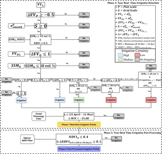
For the three study sites, the average Sentinel-1 SAR backscattering coefficients () in VV polarization and the incidence angle values ( were calculated at both plot scale and grid scale (10 km × 10 km). Since rainfall and irrigation events have the same effect on SAR values ( increases after rainfall or irrigation), this study proposes to remove or minimize the false detection of irrigation events due to rainfall events by using the mean SAR backscattering signal at grid scale (10 km × 10 km). The SAR signal at grid scale obtained from bare soil areas with low vegetation cover is assumed be a descriptor of rainfall events. For the plot scale, was obtained by averaging the backscattering coefficient in the linear unit of all the pixels within each plot. For the grid scale, was obtained by averaging values in a linear unit of all agricultural bare soil pixels existing within each grid cell. The average backscattering coefficient, at plot and grid scales, helps reduce the speckle noise in the SAR data. Moreover, at each available S2 image, the average NDVI values were calculated for each plot and grid cell (10 km × 10 km). The proposed methodology consists of two major phases. Phase 1 consists of the tree-based conditions applied over σ°-values at both plot and grid scales in which, at a given SAR date, each plot is evaluated for encountering or not an irrigation event. Phase 2 is a post-processing phase where the irrigation events obtained in Phase 1 at each plot were filtered using additional criteria based on optical data. In order to ensure near real-time detection in phase 1, the absence or presence of an irrigation event at each plot for a given SAR time is evaluated using only the SAR temporal series collected in previous dates (only before ) at each plot. However, the optical filter in phase 2 requires subsequent optical data one month after the SAR date. The significance of each proposed filter (criteria) is discussed separately in the coming sections and finally a practical overflow of the whole chain is presented.
3.2. σ° SAR Backscattering at Plot Scale
The proposed method is based on detecting the change in the backscattering coefficient at plot scale. When the surface soil moisture (SSM) increases between two consecutive SAR acquisitions, -value between these two dates increases. Since irrigation is an artificial application of water, it causes obviously an increase in the SSM values. Thus, the SAR -value could increase between two SAR dates if an irrigation event occurred between these two SAR acquisitions [21,22]. It is good to mention that only the VV polarization was considered in this study since VV is more sensitive to the soil water content than VH which is more sensitive to the vegetation cover [32].
Not only could the increase in the -values be an indicator of an irrigation event, but also the stability or a slight decrease of -values between two dates could be linked to an irrigation event if the -values attain high values. In fact, with no actions, such as irrigation, rainfall, soil work, or vegetation development, the SAR signal between two near dates (at maximum 6 days) tends to decrease, especially during spring and summer season, due to several water cycle parameters such as the infiltration, evaporation and evapotranspiration that cause a decrease in the SSM values. Thus, stabilization or slight decrease of between time and time could be evidence of an additional water supply if and only if the level of the SAR signal at is already high due to a previous irrigation or rainfall event occurring at time.
Since the method is based on detecting the change is values, we propose to calculate, at each SAR acquisition, the difference between the value at this acquisition and at the previous SAR acquisition. We calculate therefore at plot scale as:
where is the in VV polarization at the present SAR date and is the in VV polarization at the first previous date.
Finally, for the value, three main thresholds were determined for probable irrigation events. First, if is less than or equals −0.5 dB (which correspond to a decrease in -value more than 0.5 dB), then we assume that no chance of irrigation exists. If the is greater than or equal to 1 dB, then a possible irrigation event could have existed. In addition, if the is between −0.5 dB and 1 dB (stabilization or slight decrease) then an irrigation event could have also existed. However, it is necessary to add other criteria to confirm the possible irrigation event between date and . These additional criteria will be discussed in the coming sections.
3.3. σ° SAR Backscattering at Grid Scale
The increase in the SSM values could not only be attributed to an irrigation event but also to rainfall events that are the main contributor in the SSM variation. Then, a good separation between rainfall events and irrigation events should be also performed. Actually, rainfall events and irrigation events are both considered as water supplements and thus may have the same effect on the value of . For example, the threshold value of (presented in Section 3.2) could be a result of a rainfall event and not only an irrigation event. Therefore, the ambiguity between rainfall and irrigation is the principal factor to be resolved for a good detection of irrigation events. Thus, better detection of irrigation events requires information about rainfall.
In this study, information about rainfall has been determined through the σ° value obtained at grid scale (10 km × 10 km). We assume that if the bare soil plots with low vegetation cover within the spatial extent of 10 km × 10 km show an increase of the SAR backscattering signal (increase in SSM values) between two consecutive radar acquisitions, a rainfall event probably occurred. This correlation between rainfall and has been presented by Bazzi et al. [33] where they compared SSM estimations at bare soil plots in 10 km grid scale to rainfall events at the same scale and concluded that strong consistency exists between rainfall events and SSM values at 10 km grid scale. Moreover, Bazzi et al. [12] used the SAR signal at grid scale conjointly with the SAR signal at plot scale to map irrigated areas at plot scale. They reported that the use of has remarkably improved the classification accuracy of irrigated/non-irrigated plots by 15%.
The SAR backscattering coefficients at grid scale are obtained by averaging σ° values of all bare soil pixels within each grid cell (10 km × 10 km). A mask for bare agricultural soil pixels has been determined using first a land-cover map to delineate only agricultural areas (excluding urban, forests…) and then a threshold applied over the NDVI values obtained from S2 images. For this reason, the land-cover map proposed by Inglada et al. [34] is used for the two French sites while the agricultural plots of the SIGPAC data have been used for the Catalonia site. A maximum NDVI value of 0.4 is fixed to extract bare soil pixels with low vegetation cover. Thus, at each SAR date, and for each grid cell a value is obtained describing the σ° backscattered from bare soil pixels of agricultural areas only within each grid cell (10 km × 10 km).
At a given date, the change in SAR σ° at each 10 km cell could be obtained through the difference of σ° value at the given date and the σ° at the first previous date
where is the in VV polarization at the present SAR date and is the in VV polarization at the first previous date.
Using a threshold value of , rainfall events could be determined and irrigation events detected in Section 3.2 could be filtered. First, the grid based filters are only applied in the case where has a value more than or equal to −0.5 (Section 3.2) (probable irrigation event). We consider that if the is greater than 1 dB then a rainfall event occurred and, therefore, there is no chance of irrigation detection regardless of the value of . This filter helps reduce an important part of the ambiguity between rainfall and irrigation. Next, we consider that if the value of is between 0.5 and 1 dB (low rainfall possibility), then a probability of irrigation can exist based on the value of . In this case, if is less than 0.5 dB then irrigation did not take place (at 10 km bare soil plots have slightly increased more than that at the plot scale). On the other hand, if the value of is greater than 0.5 dB, then we calculate the difference ( between and (). If the value of is greater than 1 dB, then irrigation has more chance than rainfall and the point is assumed corresponding to an irrigation event. Inversely, if is less than 1 dB then no irrigation occurs. The indicator was also used to help confirm whether a point is an irrigation event or not in the case of slight change in (. When the value of is between 0 and 0.5, the value of must be greater than or equal to 1.5 dB in order to consider the point as an irrigation event. Similarly, should be greater than or equal to 2 dB if the value of is between −0.5 and 0.
Finally, we consider that if the value of is less than 0.5 dB, then irrigation could be detected in case the value of respects certain criteria which will be detailed in Section 3.7.
3.4. Reducing Vegetation Contribution
Over vegetated areas, is not only affected by the soil water content but also by the characteristics of the vegetation cover. Indeed, for certain agricultural crops, the SAR backscattering signal is attenuated by the existing vegetation cover [32,35]. For example, for crop types such as soya, sorghum and sunflower the SAR backscattering signal between two dates could increase due to the development of the vegetation cover. The direct effect of vegetation cover on the SAR signal should be also considered to ensure accurate detection of irrigation events.
Recently, Nasrallah et al. [36] used a smoothed Gaussian filter on SAR temporal series in order to describe the phenology stages of the vegetation growth over wheat crops. They demonstrated that the smoothed Gaussian could be used to describe the vegetation contribution in the SAR temporal series over wheat plots. Therefore, to minimize the effect of vegetation growth on the radar signal, we propose to smooth the temporal series of the SAR backscattering signal. This smoothing gives the general behavior of the vegetation contribution in the SAR signal. However, in order to ensure the near real-time detection of irrigation, we propose to smooth the signal only using SAR dates existing before the examined SAR date. This means that at each SAR date, a smoothing value is obtained by applying a Gaussian smooth on all points before this date (from to). In this study, the multidimensional Gaussian smooth has been used and the standard deviation for the used Gaussian kernel was set equal to 4. Finally, we obtain the index considered as a vegetation descriptor where:
Therefore, if is less than (i.e., , then the point should not be further considered for irrigation detection. This smoothing allows us to determine a vegetation indicator capable of reducing the vegetation effects in the SAR signal (at each date) without losing possible irrigation events.
Another vegetation contribution filter has been suggested particularly for winter cereals usually grown in the period between September and July of each year (wheat, barley and oats). In their study over wheat crops, Nasrallah et al. [36] showed that the C-band SAR backscattering signal in VV polarization decreases gradually between the germination phase occurring by the beginning of January and the heading phase occurring between mid-March and mid-April. In the heading phase, the C-band SAR backscattering signal attains extremely low values due to extreme vegetation attenuation (less than −15 dB for incidence angle between 32° and 34°). The gradually increases then, between mid-April and the end of May, when cereals move from the heading phase to the soft dough phase. This increase in the C-band SAR signal is mainly due to the change in the phenology phase of the cereals and is not linked to irrigation episodes. To reduce this ambiguity, we propose to eliminate detected irrigation points between mid-April and the end of May if and only if attains extremely low value (less than −15 dB) between mid-March and mid-April. In this way, we can ensure that these detected points are most probably a phenology change of cereals where increases from extremely low values between March and April ( to higher values in May. Practically, for any plot, if a point is detected between mid-April and the end of May, we find the minimum of all values (denoted by ) acquired between mid-March and mid-April. If the value is less than −15 dB (most probably heading phase of cereals), then we eliminate the detected point.
3.5. Surface Soil Moisture Filter
As discussed in Section 3.2, irrigation activities obviously cause an increase in the SSM values at plot scale. Thus, an important factor that can describe the presence or absence of irrigation events is the SSM value. We consider here that low soil moisture values are not correlated with an occurring irrigation event since irrigation must increase the SSM values especially over plots with small vegetation cover. However, the integration of any proposed SSM filter requires proper estimation of SSM values. Recently, an algorithm using the neural network (NN) technique was developed by El Hajj et al. [32] to estimate SSM values at plot scale over agricultural areas with vegetation cover. In their study, SSM values were estimated with an accuracy of 5 vol.% (volumetric water content in percent = 0.05 ) over agricultural areas which is considered a pleasant accuracy for any hydrological application at plot scale. In addition, the NN developed by El Hajj et al. [32] has showed the most accurate SSM estimations when evaluated against several SSM products such as the Soil Moisture and Ocean Salinity (SMOS), Soil Moisture Active Passive (SMAP) [37] and Copernicus Surface Soil Moisture (C-SSM) [38].
In this study, the NN developed by El Hajj et al. [32] has been used to estimate SSM values at plot scale. The NN requires as input data: SAR signal in VV polarization, the SAR incidence angle, and an NDVI value. As a result, SSM values were estimated at each plot and for each SAR date denoted by . However, in another study, El Hajj et al. [39] recommend that the SSM estimation could be limited in the presence of very dense vegetation cover due to the high vegetation attenuation on SAR signal. Thus, has only been considered for NDVI values less than 0.5. Finally, an additional filter is applied in which irrigation points have been restricted to SSM estimation 15 vol.% when the NDVI value is less than 0.5. For NDVI values greater than 0.5, the SSM filter was not applied.
SSM values at plot scale were also used to help confirm whether a point is an irrigation point or not in the case of slight change in (. As presented in Section 3.2, the stability or slight decrease of the SAR signal at plot scale between and could be interpreted as an irrigation event if and only if the at time already attains high values (due to irrigation or rainfall). To ensure this situation, we say that at time, SSM estimation should be greater than or equals to 20 vol.% in order to guarantee that humid soil conditions at time have continued to time .
Over the grid scale, the SSM estimation for the obtained for bare soil plots with low vegetation cover (NDVI <0.4) at grid scale (Section 3.3) was also performed at each grid cell and for each SAR date . This estimation presents the surface water content over bare soil plots on the basin scale. In fact, we assume that high soil moisture values at grid scale (10 km × 10 km) are more likely to be linked to possible rainfall events rather than irrigation events (humid soil conditions at grid scale). For this reason, we propose to eliminate all the points where the SSM estimation at grid scale is greater than 20 vol.%. For the grid scale, the effect of vegetation attenuation on SSM estimations (high NDVI values) does not exist since the -values were only calculated for bare soil plots with low vegetation cover.
3.6. Optical Normalized Differential Vegetation Index (NDVI) Filter
During the sowing or harvesting periods, the cropland plots usually encounter an increase in the surface roughness due to soil work. In fact, the backscattered radar signal strongly depends on the geometric characteristics such as the surface roughness that is usually expressed by the height root mean square (Hrms). The Hrms is the standard deviation of surface height (root mean square) which specifies the vertical scale of surface roughness. Several studies have discussed the sensitivity of the radar backscattering signal to the surface roughness [40,41,42]. Baghdadi et al. [43] reported that a difference of 4 dB could be observed between backscattering signal from smooth surface (Hrms = 0.5 cm) and rough surfaces (Hrms = 3 cm). Therefore, between two near-date SAR acquisitions, an increase in the surface roughness could cause an increase in the backscattering coefficient. This increase is related to the change of the geometrical characteristics of the soil and not to the change of the water content (irrigation or rainfall). To overcome this limitation, an additional optical filter is suggested in order to better distinguish irrigation peaks from soil works such as sowing or harvesting.
Generally, irrigation activities must occur during a crop-growing cycle. This means that irrigation must be followed by a development of the vegetation cycle. When croplands receive water, high soil moisture causes better photosynthesis resulting in an increase in the leaf area index (LAI) values and therefore an increase in the NDVI values [6]. Therefore, we consider that an irrigation event should be followed by the development of NDVI values. For this reason, a post processing filter is proposed to eliminate some false detected irrigation events due to soil work. At each plot and for each detected irrigation event (at a given SAR date), we first obtain the difference between the NDVI value at the detected irrigation event and the next NDVI value of the next optical image (after 20 to 30 days according to cloud limitation):
where is the NDVI value at the current SAR date and is the NDVI value one month later.
The value is considered as a vegetation indicator which helps in detecting whether an increase of the NDVI values is observed or not (growing cycle) after the probable detected irrigation event. The filter suggests that if the value is less than 0.4 (bare soil conditions with small vegetation cover) and , then the point is a falsely detected irrigation point and is eliminated. For greater than 0.4, the filter is discarded because in the presence of vegetation the existence of irrigation event is more probable. This filter ensures that if the bare soil condition is permanent and a vegetation growth cycle does not exist (or was in a decreasing stage), then the detected event is most likely to be a soil work point and not an irrigation point. However, this filter is a post-processing filter that can be applied after obtaining another NDVI image after 20 to 30 days.
3.7. Global Overflow for Irrigation Event Detection
Figure 3 presents a detailed overflow of the proposed tree-based change detection methodology. For a given plot and at a given SAR image acquired at time, seven main indicators could be extracted for the plot:
- Change in SAR signal at plot scale
- Change in SAR signal at grid scale
- : Smoothed vegetation descriptor
- : SSM value at plot scale
- : SSM value at plot at grid scale containing this plot
- : NDVI value at time
- : Vegetation growth indicator
The chain starts with the value where a value less than −0.5 dB is considered as the non-irrigation point. If the value of is greater than −0.5 dB, the smoothed vegetation descriptor is then checked for being positive and the point is considered as non-irrigation if. If is positive, the is then checked for the threshold value of 15 vol.% and the point is considered as non-irrigation if the with (both conditions should occur simultaneously). When the studied point arrives to pass by all the previous filters, the chance of having a water supplement (irrigation or rainfall) increases, and thus the change of SAR signal at grid scale is required at this stage in order to eliminate the irrigation-rainfall ambiguity. Filters applied at grid scale could be divided into four main cases:
- Case i: If then a rainfall event have occurred and the point is not an irrigation point.
- Case ii: If then a rainfall event probably occurred before and there is low chance to have an irrigation event (humid soil conditions at basin scale).
- Case iii: If we check the value of for two cases:
- ❖
- Case iii.1: Ifthen no irrigation took place.
- ❖
- Case iii.2: If and then it is considered as irrigation point with high certainty.
- Case iv: If then we check the for four different cases:
- ❖
- Case iv.1: then the point is an irrigation point with high certainty.
- ❖
- Case iv.2: then the point is an irrigation point with medium certainty if and only if OR .
- ❖
- Case iv.3: then the point is an irrigation point with low certainty if and only if OR .
- ❖
- Case iv.4: then the point is an irrigation point with low certainty if and only if AND the previous point at is a high certainty irrigation point or a rainfall point ().
A certainty indicator of irrigation (high, medium and low) is also associated for each detected irrigation point. The high certainty irrigation points are associated for the points considered as irrigation points from cases iii.2 and iv.1 (significant increase in). For the points of case iv.2 a medium certainty is associated, while low certainty is considered for irrigation points detected from cases iv.3 and iv.4.
The implementation of the proposed method in a near real-time scenario depends principally on the delivery time of S1 images. S1 images are usually delivered by ESA in a “fast 24 h” delivery mode. This mode insures that the S1 image is available for download 24 h after the satellite acquisition. Considering that the pre-processing of S1 images and applying the proposed method could be automatically performed with minimum human involvement, the irrigation event could then be detected about one hour after receiving the S1 images.
Finally, the post NDVI filter (Section 3.6) is applied for each detected irrigation point in order to eliminate the ambiguity with soil work. When another NDVI image is acquired at, the is calculated. Then, for each detected irrgation event, if and , then this irrigation event is eliminated. This NDVI filter is a long-term real-time scenario because it requires obtaining a new NDVI value one month later. Therefore, this optical filter remains as a post processing of the obtained irrigation points.
It is important to mention that the methodology is applied separately for the ascending (evening overpass) and descending (morning overpass) SAR acquisitions. In fact, morning and evening acquisitions could not be joined in one temporal series due to the presence of the diurnal variations between the two acquisitions. The diurnal variation is a result of the difference in the vegetation water content (VWC) between the morning and the evening. This difference in VWC causes high difference in the radar backscattering signal over vegetated plots between the morning and the evening acquisitions. Several studies have reported that in the morning overpass registers higher values than in the evening overpass [44,45,46]. Therefore, it was suggested to investigate separately each SAR temporal series acquired in the morning and evening.
4. Results
4.1. Grid Scale σ° Temporal Profile
Since irrigation and rainfall events are both considered a water supplement and have the same effect on the SAR backscattering coefficients, it was proposed to minimize the irrigation-rainfall ambiguity using the σ° values obtained at basin scale (10 km × 10 km). Figure 4 shows an example of the temporal behavior of SAR values in VV polarization obtained at a 10 km grid cell (red curve) for Montpellier (Figure 4a), Tarbes (Figure 4b) and Catalonia (Figure 4c). Daily precipitation records obtained from the Global Precipitation Mission (GPM) data are added to the figures (blue curve) to help understand the consistency between the grid scale values and the rainfall events. The green line shows the SSM estimation at grid scale (for bare soil plots with low vegetation cover) at each SAR date while the dotted black line shows the threshold value fixed for at 20 vol.%. Following a rainfall event, the value increases (more than 1 dB) due to important precipitation before the SAR acquisition (black dashed circle) accompanied with high SSM estimations (more than 20 vol.%) indicating humid soil conditions at 10 km scale. On the other hand, the absence of precipitation causes a decrease or stability of σ° value at grid scale with low soil moisture values (less than 15 vol.%) indicating dry soil conditions (yellow dashed circle). This consistency between rainfall, and SSM estimations at grid scale ensures that both and SSM estimations at 10 km scale are a good representative for rainfall events and, therefore, could be used to eliminate the uncertainty between rainfall and irrigation.
4.2. Results over Montpellier
Figure 5 presents the results of the application of the proposed methodology (Phase 1 and 2) over the three plots P1, P2 and P3 located in Montpellier, France using the ascending (morning) and descending (evening) SAR images separately. Over Montpellier site, the morning acquisition is 36 h prior to the evening acquisition.
Figure 5a,b show the morning and evening SAR acquisitions for P1 plot (maize), respectively. The first detected irrigation point was on 17/07 (morning acquisition) and 18/07 (evening acquisition) due to two irrigation episodes that took place on 16/07 and 18/07. Between 19/07and 31/07 no irrigation occurred on the plot and no peaks where detected for two consecutive SAR acquisitions. Later, on both 05/08 (morning) and 06/08 (evening), an irrigation peak was detected due to two irrigation episode occurring on 03/08 and 04/08. In addition, two irrigation episodes that occurred on 04/09 and 05/09 appeared as an irrigation peak on the evening image of 06/09. However, the morning image acquired on 04 September 2017 did not show any detected irrigation since the episodes occurred after the SAR acquisition (SAR acquired at 06h00 while irrigation generally takes place after 09h00). Moreover, an irrigation episode occurring on 11/09 was detected on the evening image acquired on 12 September 2017. Two irrigation episodes occurring on 13/09 and 14/09 appeared on both the morning and evening acquisitions on 14/09 and 15/09, respectively. By combining the irrigation events detected from the morning and evening acquisition, 12 out of 15 possible irrigation episodes over P1 were detected including 5 points with high certainty, 5 points considered as medium certainty and 2 points with low certainty. However, it is important to mention that several irrigation episodes occurring between two consecutive SAR dates are considered as only one irrigation episode. For plot P1 only one point with low certainty was falsely detected as irrigation event.
For the soya plot (P2), the results of the combined use of the morning (Figure 5c) and evening (Figure 5d) acquisitions show that 11 irrigation episodes were detected out of 13 possible irrigation episodes. Among the 11 detected irrigation points, eight points were with high certainty, two medium and one low certainty point. Moreover, among the 92 SAR acquisitions (morning and evening), only one false irrigation detection was obtained with low certainty. The first irrigation episode on 29/05 was detected in the morning SAR image of 31/05 (Figure 5c). For the morning acquisition, the radar signal then decreased between 31/05 and 06/06 due to the decrease in soil moisture but started to increase between 06/06 and 24/06 without any rainfall or irrigation events. This increase in the values for three consecutive acquisitions was strongly correlated with the development of vegetation cover (NDVI values increases sharply during this period). However, among these three SAR points, two points were correctly not detected as irrigation points since they were filtered by the smoothed Gaussian filter that helped eliminate the effect of the vegetation development on . Figure 6 explains the effect of the smoothed-Gaussian filter over P2 plot of Montpellier where the (red curve) is added to the results obtained by Figure 5d to demonstrate the importance of the smoothed-Gaussian filter. In Figure 6, the green dashed circle shows the three consecutive increase of between 06 and 24 June 2017. However, for two out of these three points, the curve is above curve thus the calculated value is negative and these points were not detected as irrigation points.
The sorghum plot (P3) encountered five irrigation episodes between 31 May 2017 and 10 August 2017 (Figure 5e,f). Using the proposed change detection method, five out of the five episodes were correctly detected as irrigation events. The first irrigation episode was detected on the evening SAR image (Figure 5f) of 01/06 due to an irrigation event occurring on the same date. Then, the 4 irrigation episodes that occurred on 26/06, 07/10, 27/10 and 10/08 were detected with both acquisition modes (ascending and descending). However, on this plot two false irrigation points were detected with medium and low power.
Table 2 summarizes the results obtained on the three plots of Montpellier site. The total number of irrigation events over the three plots was 48 events. However, at each plot, several irrigation events occurring between two consecutive SAR dates are considered as only one irrigation event. We call these events the possibly detectable irrigation events. For example, three irrigation events occurring on 10/08, 11/08 and 13/08 on plot (P1) are considered as one irrigation event since the three events were followed by only one available SAR acquisition on 13 August 2017. Therefore, among the 48 irrigation events occurring on the three plots, 33 events could be possibly distinguished by the acquired SAR temporal series. This means that, 69% of the total number of irrigation events could be detected by the available SAR temporal series. Out of 33 possibly detectable irrigation events over the three plots, 28 irrigation episodes have been correctly detected. This means that among the possible detectable irrigation events 84.4% of these events are correctly detected. However, a total error of five falsely detected irrigation events has been registered over the three plots. The falsely detected irrigation points corresponds to the saturation of the radar signal caused by very well developed vegetation cover in plots P1 (maize) and P3 (Sorghum).
4.3. Results over Catalonia
Over the Catalonia region, the huge database available allows us to investigate in depth the performance of the proposed method. The method was applied not only over irrigated plots but also over non-irrigated plots in order to analyze its capability to distinguish between irrigated and non-irrigated fields. First, it is important to remember that Catalonia region is a semi-arid region with a dry summer where most of the irrigation activities occur during the summer season (between May and September). Figure 7 presents the temporal profile of and over the period between September 2017 and December 2018 (evening acquisitions) along with the irrigation points detected during this period for an irrigated maize (Figure 7a) plot, irrigated alfalfa plot (Figure 7b), and non-irrigated wheat plot (Figure 7c). The daily GPM precipitation data are also presented in the three figures (blue curve). During the period between September 2017 and December 2018, 11 irrigation points were detected on the maize plot whereas 12 irrigation points were detected on the alfalfa plot. In both irrigated plots (Figure 7a,b), the irrigation points correspond to the dry summer period (between 25 April and 30 September). For example, 6 irrigation points were detected on the maize plot (Figure 7a) between 12 June 2018 and 15 August 2018. This is correlated with the existence of the maize vegetation cycle in the summer season (Increasing NDVI values). The alfalfa plot (Figure 7b) shows also frequent irrigation points detected between 12 June 2018 and 30 August 2018. For both maize and alfalfa plots, the between 01 June 2018 and 30 September 2018 shows stable low values indicating dry conditions and the absence of rainfall events. On the other hand, the frequent change of the in both plots indicates that possible irrigation events have occurred. This increase of the was detected as irrigation events based on our proposed method.
Over the non-irrigated wheat plot presented in Figure 7c, no irrigation points have been detected for 82 SAR images (18 months). Such results support our criteria for detecting irrigation events and eliminating ambiguities with rainfall or vegetation effects. Following a rainfall event both and increase and then decrease following a dry period. The consistency between both and for the non-irrigated plot during the whole period indicates that the plot did not receive any water supplement other than rainfall events. Despite several frequent changes of the over the complete temporal series due to several rainfall events and vegetation change, the method was able to eliminate all possible irrigation ambiguities and judge that the plot did not receive any irrigation event.
An important point regarding the wheat plot in Figure 7c is the period between 19 April 2018 and 13 May 2018. During this period, the SAR backscattering signal increases gradually between each two SAR dates (red dashed circle). This increase in the SAR signal is related to the transition between the heading phase (minimum point on 19/04) and the soft dough phase (maximum point at 19/05). However, these points were eliminated using the proposed cereal phenology filter discussed in Section 3.4.
The proposed method was applied over a wide area of Catalonia region including 159,850 plots (123,428 non-irrigated and 36,423 irrigated plots) of different crop types. Despite the absence of information about the exact irrigation dates over Catalonia, a quantitative analysis was performed by comparing the results obtained by applying the method over irrigated and non-irrigated plots. Over Catalonia, the morning acquisition was 12 h prior to the evening acquisition. Figure 8 presents the histogram of the distribution of the number of events detected over irrigated and non-irrigated plots. Figure 8a corresponds to the morning SAR acquisition and Figure 8b corresponds to the evening SAR acquisition. The intersection between the evening and morning acquisitions is presented in Figure 8c. The intersection means that at each SAR date the point is considered as irrigation point if it exists within both the ascending and the descending acquisition modes (only 12 h difference between the two acquisitions is approximately equal to same day). Finally, Figure 8d shows the result of the combined use of both acquisitions. The combination between the results of the both acquisition modes means that at a given SAR date, the point is considered irrigation point if it exists in either the ascending or the descending acquisition modes. For morning acquisition mode (Figure 8a), the distribution shows that 68.3% of the non-irrigated plots had no detected irrigation events for the period between September 2017 and December 2018 (82 SAR images). Moreover, 20.3% of the non-irrigated plots encountered only one detected event. Therefore, 88.6% of the non-irrigated plots have maximum one detected irrigation point in the morning acquisition mode. The non-irrigated plots with 2 and 3 detected irrigation points represent only 6% and 2% respectively. On the other hand, only 12.1% of the irrigated plots failed to register any irrigation event. Thus, 87.9% of the irrigated plots had one and more detected irrigation points. The percentage then increases gradually where 54.9% of the irrigated plots had between two and five detected irrigation points. In addition, 20.4% of the irrigated plots encountered between five and 10 detected irrigation points. Similar results are obtained for the evening acquisition (Figure 8b). For example, 58.2% of the non-irrigated plots had no detected irrigation events while 25.1% had only one detected event. Thus, 83.3% of the non-irrigated plots encountered a maximum of one detected point for evening acquisition mode. In contrast, only 9.1% of the irrigated plots failed to gain any detected irrigation point and therefore 91.9.% of the irrigated plots had one and more detected irrigation point in the evening acquisition mode. Moreover, 51.1% of the irrigated plots had between two and five events and 27.3% of the irrigated plots had between six and ten detected points.
The intersection between the morning and evening acquisitions modes (Figure 8c) shows that 90.2% of the non-irrigated plots have no detected peaks whereas 72.4% of the irrigated plots had one or more detected irrigation peak. The combination of both acquisition modes (Figure 8d) increases the number of detected irrigation points but leads to an accuracy of the same order of magnitude as in the case of a separate use of the two SAR acquisition modes or in the case of the intersection of the two acquisition modes. For non-irrigated plots, 45.9% of the plots had no detected points and 27.0% had one detected points. The percentage decreases gradually to then reach 7% for three detected irrigation points. Inversely, the irrigated plots with no detected irrigation points consist of only 6.8% while the percentage of plots varies between 5% and 10% for irrigation points between 1 and 14 points.
Figure 9 represents the distribution of the number of irrigation points detected over irrigated plots in Catalonia, Spain as a function of months. For each month (including approximately five SAR acquisitions at each acquisition mode), the number of irrigation peaks detected over all the irrigated plots is calculated. While Figure 9a represents the distribution of irrigation points for the morning acquisitions, Figure 9b shows this distribution for the evening acquisition. For the morning acquisition mode (Figure 9a), the number of irrigation points reaches a low value in February 2018 (1040 points ~0.7%) and then starts to increase gradually between March 2018 and May 2018. A sharp increase of the irrigation points exists between May 2018 (3827 ~3%) and June 2018 (21,787 ~16%) and then continues to increase to reach a maximum value in July 2018 (25,380 ~19%). In August 2018, the number of irrigation points slightly decreases to attain approximately 15%. Then the number of detected irrigation points starts to decrease until reaching a minimum value in November 2018 (103 ~0.01%). Similar behavior is registered in the evening acquisition (Figure 9b) where the number of irrigation points reaches low value in February 2018 (2735 ~1%) and then increases until reaching its maximum value in July 2018 (29,286 ~18%). A slight decrease is recorded in August 2018 (27,252 points ~16%). The number of detected irrigation points then starts to decrease to reach a minimum value of 257 points ~0.01% in November 2018.
As a result, Figure 9 shows that most of the detected irrigation points exist within the period between March 2018 and September 2018. Indeed, 80.0% of the total detected points using the evening acquisition mode (Figure 9b) exist within the period between 01 March 2018 and 30 September 2018. Similarly, 74.5% of the total detected points exist within the same period for the morning acquisition mode (Figure 9a). Only 12% of the irrigation points (in both morning and evening) correspond to the period between November 2017 and February 2018. This low percentage mostly corresponds to the false detection of irrigation events since irrigation rarely occurs over this period and rainfall events are abundant. Therefore, the results show that most of the detected points using our proposed irrigation detection method correspond to the dry season where irrigation mostly occurs in the region.
4.4. Classifying Irrigated and Non-Irrigated Plots over Catalonia
Based on the results obtained in Section 4.3, we propose to classify irrigated and non-irrigated plots over the Catalonia site using the obtained distributions of detected irrigated points present in Figure 8. Four different classifications were performed. The first classification was performed using the results obtained from the morning SAR acquisitions (Figure 8a), and the second classification was executed using the results of evening SAR acquisitions (Figure 8b). A third classification was undertaken using the intersection between the morning and evening results (Figure 8c), and finally a fourth classification was executed using the combination of the morning and evening results (Figure 8d). As stated in 4.4, the intersection means that at each SAR date, a point is considered an irrigation point if it exists in both SAR acquisition modes while the combination means that the point is considered as irrigation point if it exists in either one of the two modes. For the morning and the evening classification scenarios, we suppose that a plot is considered irrigated if our method identifies two and more irrigation points within the complete SAR temporal series (morning or evening). For the intersection classification scenario, we consider that a plot is an irrigated plot if the intersection between the morning and the evening results gives one and more irrigation points. Finally, for the combined classification we consider that a plot is irrigated if the combination of the morning and the evening results gives three and more irrigation points. For each of the four classifications, a confusion matrix is built and Table 3 reports the accuracy metrics by means of the overall accuracy, weighted F-measure, and the F-Measure at each class (irrigated, non-irrigated). The overall accuracy is a standard metric used for remote-sensing applications. The weighted F-measure corresponds to the harmonic mean affected by the number of samples. Since the number of non-irrigated plots is bigger than the irrigated plots, the weighted F-measure is well suited to evaluate the performance of the classification [47].
The highest overall accuracy (85.9%) was recorded for the intersection scenario with a weighted F-measure of 86.0%. The F-score of the irrigated class in the intersection scenario reaches 0.70 and that for the non-irrigated class reaches 0.90. On the other hand, the lowest overall accuracy was recorded for the evening SAR acquisition (82.5%) accompanied with the lowest weighted F-measure (83.4%). The combined scenario shows the highest accuracy for the irrigated class (F-measure = 0.72) with an overall classification accuracy of 85.4%. Generally, the F-measure of each class was nearly the same between the four scenarios. In fact, the F-measure varies between 0.68 and 0.72 for the irrigated class, and varies between 0.88 and 0.90 for the non-irrigated class.
The four proposed classification scenarios were re-established using only the detected irrigation events between April and September 2018 which corresponded to the irrigation period in Catalonia. Figure 10 shows a comparison between the accuracy metrics previously obtained when using all the detected irrigation events (between September 2017 and December 2018) and that obtained when using only irrigation events between April 2018 and September 2018. For the morning and evening classification scenarios, the results show that the overall accuracy increased by 2.8% and 4.8%, respectively, when considering only detected irrigation events between April and September (Figure 10a). The F-measure of the irrigated class increased by 2.2% for the morning scenario and significantly increased by 5.0% for the evening classification (Figure 10b). For the intersection scenario, the obtained results remained nearly the same for the four accuracy metrics. Moreover, in the combined classification scenario, the overall accuracy increased by 4.0% (Figure 10a) where the F-measure of the irrigated class increased by 4.5% (Figure 10b). The F-measure of the non-irrigated class (Figure 10c) also increased for the four different scenarios. Finally, the weighted F-measure also increased by 2.0%, 4.0% and 3.4% for the morning, evening and the combined classification scenarios, respectively (Figure 10d). Therefore, a priori information about the irrigation period can help reduce the uncertainty in the proposed model for better irrigation detection. This priori information helps limiting the size of the studied temporal series and thus reduces the chance of detecting additional false irrigation events.
4.5. Results over Tarbes
The proposed method was applied over irrigated plots in Tarbes, south-west France. Figure 11a represents the and in the morning acquisition mode for an irrigated maize plot with the irrigation points detected using the proposed change detection method. While Figure 11a shows the complete series between 01 March and 30 November 2017, Figure 11b represents the period where the irrigation points were detected. However, irrigation dates were not available over this site so a qualitative analysis was performed to show the performance of the method. During the period between 01 March 2017 and the end of June 2017 (Figure 11a), the and followed the same behavior for almost all the dates. Following a rainfall event both curves increased and then decreased following a period without rainfall. This consistency could be related to the absence of any additional water supplement on the plot scale. However, between March and mid-May, the NDVI values were low (less than 0.2) indicating bare soil conditions. This also supports the possibility that no irrigation had occurred for this period. The NDVI then started to increase showing a vegetation cycle between May and October. Using the proposed method for detecting irrigation events, four irrigation points were detected over this plot (Figure 11b). In general, all these irrigation points corresponded to an important increase of accompanied with absence of rainfall events as shown by the GPM data (blue curve) and the -values at grid scale (pink curve). For example, an important cumulative rainfall of approximately 40 mm three days before the SAR image acquired on 28 June 2017 caused to increase by 2.5 dB. Six days later, no rainfall events were registered and the decreased by 1.5 dB. For the same period, increased by 1 dB. This point was the first irrigation point detected on the plot. Similarly, between 10/07 and 16/07, decreased by 2.1 dB due to the absence of precipitation while increased by 1.1 dB indicating that a water supplement could have occurred. The absence of precipitation for 12 days between 22/07 and 04/08 caused to decrease gradually. However, the SAR image acquired on 04/08 showed an increase of the SAR signal at plot scale which was evidence of an irrigation event occurring. Likewise, between 15/08 and 21/08 the increased by 1.5 dB indicating the presence of irrigation event along with a stability of low (~−11.5 dB) indicating the absence of any rainfall events. After the fourth detected point on 21/08, the NDVI started to decrease. Usually during this phase irrigation events rarely occur. After 02/09, the σ° values at both plot and grid scale regained their consistent behavior indicating the absence of irrigation. Finally, it is important to mention that the summer season in Tarbes is humid and encountered several rainfall events.
Figure 12 presents the histogram of the distribution of the number of events detected over irrigated plots in Tarbes for morning acquisition (Figure 12a), evening acquisition (Figure 12b), intersection between morning and evening acquisitions (Figure 12c) and the combination of both acquisitions (Figure 12d). It is important to remember that the intersection means that the detected points are considered irrigation events if they exist within the morning and the evening modes while the combination means that the points are considered irrigation events if they exist in either the morning or the evening acquisition modes. Figure 12a shows that using the morning acquisition, 91% of the irrigated plots has one or more detected irrigation events and 75% of the plots have two and more detected irrigation events. Figure 12b shows that fewer points are detected in the evening acquisition than the morning acquisition where only 50% of the plots have one and more irrigation events. In Figure 12c, the intersection shows that with an interval of 36 h between both acquisitions, only 38% of the irrigation events were commonly detected within both acquisition modes. Finally, the combined use of the morning and the evening acquisitions in Figure 12d shows that 97% of the irrigated plots had and more detected irrigation events. Moreover, 90% of the irrigated plots had two and more detected irrigation events and 65% of the plots had three and more irrigation events. This indicates that the combined use of the morning and the evening acquisitions helps detect more irrigation events than using only one S1 overpass each 6 days. Figure 12d also shows that the maximum percentage of plots was registered with three irrigation events (29.7%) and the percentage then decreased as the number of detected irrigation events increase (four events and more). The low number of detected irrigation events in Tarbes, compared to those obtained over Catalonia, was expected since Tarbes is a humid region and the frequency of irrigation is less than that in the arid or semi-arid regions. Moreover, the abundance of rainfall events during the summer season could restrict the possibility of detecting all the possible irrigation events.
5. Discussion
5.1. Change Detecion in σ° SAR Backscattering
In this study, a new methodology is presented for detecting irrigation events at plot scale using the change detection in the SAR backscattering signal. The first important fact is that the change of the surface soil moisture due to irrigation events (artificial application of water) between two SAR dates may cause an increase in the SAR backscattering coefficient between these two dates. However, this assumption remains limited with the changes in SAR backscattering signal due to a rainfall event or vegetation development. Therefore, the separation between the changes in SAR backscattering signal due to irrigation events from similar changes, which could be caused by rainfall or vegetation development, was challenging.
To remove the uncertainty with rainfall events, the method proposes using the SAR backscattering signal at basin scale (10 km × 10 km) obtained from bare soil plots with low vegetation cover as a descriptor of rainfall events. The assumption stipulates that if the mean SAR signal within 10 km × 10 km grid cell increased between two consecutive dates then a rainfall event took place and thus irrigation, if it had occurred, could not be detected. This dependency between rainfall and was presented in Figure 4. For this reason, we judge that any increase in the SAR signal at 10 km grid scale by more than 1 dB is linked to rainfall events. In addition, the surface soil moisture estimation performed at grid scale was used to enhance the detection of rainfall events. Thus, a threshold of 20 vol.% for was proposed to describe humid soil conditions at basin scale which is probably linked to a rainfall event that occurred couple of days before the SAR acquisition. The combination of these two conditions at grid scale allowed a good separation between rainfall and irrigation episodes occurring at each SAR acquisition.
The second main contributor in the SAR backscattering signal at plot scale was the development of the vegetation cover. This development could cause an increase in the SAR backscattering signal at plot scale without any change in the surface soil moisture content and thus without any irrigation or rainfall events. In this study, a descriptor of the vegetation growth is suggested. This descriptor is a Gaussian-smoothing filter applied to the SAR temporal series. The values allow describing the vegetation growth pattern at the plot scale and thus permit the separation of irrigation events from vegetation growth events. This contribution of the smoothed-Gaussian is shown in Figure 6. For the soya plot (P2) of Figure 6, the vegetation descriptor helped eliminate two points considered as vegetation development points. Another vegetation development filter was proposed for cereal plots in order to remove the increase in the SAR backscattering signal due to the transition between the heading and the soft dough phenology phases. The importance of this filter was demonstrated in Figure 7c for a non-irrigated winter wheat plot. However, the date limits present in this filter (mid-March until May) could be adjusted for other geographical contexts in order to follow the cereal growth cycle where cereals could be cultivated in other months.
5.2. Effect of NDVI Optical Filter
Throughout the study, an optical post-processing filter has been suggested to ameliorate the detection of irrigation events and remove the ambiguity between the increase in the SAR backscattering signal due to irrigation events and soil work. The role of the NDVI filter is to insure that a vegetation growth cycle truly exists within or after the detected irrigation point. As presented in Section 3.6, the NDVI optical filter suggests that if the (NDVI value at a detected irrigation event) is less than 0.4 and then the point is a falsely detected irrigation point, and is further eliminated. For greater than 0.4, the filter was no longer applied because the vegetation cover is already developed (NDVI > 0.4) and the existence of irrigation event is more probable.
To assess the importance of this NDVI optical filter, we obtain first the results over Catalonia without applying the NDVI optical filter. Then we apply the NDVI optical filter using two threshold values on accompanied with the criterion. The filter was first applied using and then applied using . The results obtained previously with were also used in this comparative analysis. For each case, the threshold of was kept equal to 0.1. To present the effect of this NDVI optical filter, we intended to monitor the change in the percentage of plots that did not encounter any irrigation event for both irrigated and non-irrigated plots (0 detected irrigation events). The class with no detected irrigation events was chosen for this analysis since it describes the capability of discriminating between irrigated and non-irrigated plots. Figure 13 presents the evolution of the percentage of the plots that did not register any irrigation event as a function of the value of used in the optical filter for both morning (Figure 13a) and evening (Figure 13b) acquisition modes.
For the morning acquisition mode, Figure 13a shows that when the NDVI filter is not applied only 29% of the non-irrigated plots have no detected irrigation events. When adding the NDVI filter using (, this percentage increases to reach 44%. The optical filter applied at increases the percentage of non-irrigated plots with no detected irrigation events to reach 59%. Finally, using the NDVI optical filter at , 68% of the non-irrigated plots had no detected irrigation events. Beyond 0.4, the filter was no longer applied since vegetation already exists and the occurrence of an irrigation event was more probable than soil work. For irrigated plots in morning acquisition (Figure 13a), the percentage of irrigated plots with no detected irrigation events was 4% when no NDVI filter was added and slightly increased to 12% as the NDVI optical filter with was used. Therefore, when applying the NDVI filter using in the morning acquisition mode, the percentage of the non-irrigated plots with no detected irrigation events significantly increased by 39% (68–29%) compared to the percentage obtained when no NDVI filter was used. The percentage of the irrigated plots with no detected irrigation events increased only by 8% (12% minus 4%) compared to that obtained when no NDVI filter was used.
For the evening acquisition mode (Figure 13b) the results show that the percentage of non-irrigated plots with no detected events increased from 22% when no filter was applied to reach 35%, 49% and finally 58% when the and were used respectively. For the irrigated plots in evening acquisition, the percentage increased from 3% when no filter was applied to reach 9% when NDVI optical filter was applied at . Therefore, when applying the NDVI filter using in the evening acquisition mode, the percentage of the non-irrigated plots with no detected irrigation events increased by 36% (58–22%) compared to the percentage obtained when no NDVI filter was applied. On the other hand, the percentage of the irrigated plots with no detected irrigation events increased only by 6% (9–3%) compared to that obtained when the filter was not applied.
The significant increase in the percentage of non-irrigated plots with no detected peaks, between the case where NDVI filter was not applied and NDVI filter was applied at , encouraged the use of the post-processing optical filter despite of the loss of 8% and 6% in the irrigated plots for morning and evening acquisitions, respectively.
5.3. Strengths, Limitations and Future Directions
The results of the study demonstrate that irrigation events could be detected using the Sentinel-1 satellite data with 6 days temporal resolution. Using the proposed method, the spatial distribution of the plots that encountered an irrigation event could be obtained at each available SAR acquisition. Currently, the Sentinel-1 satellite is the only operational satellite that provides SAR data with high revisit time (6 days). However, this revisit time could still affect the detection of irrigation events. The first limitation of the proposed method is the effect of the time lag between the irrigation episode and the satellite passage. In fact, the detection of irrigation can become difficult if the irrigation event takes place more than three days before the SAR acquisition. Hajj et al. [21] showed that irrigation could be detected if the irrigation took place three days and less before the radar acquisition. In their study using X-band SAR data, they showed that more than three days after the irrigation event, the surface soil moisture could attain the same value as that before the irrigation due to evaporation. Thus, a SAR acquisition more than three days after the irrigation event could not show any change in the surface soil moisture and the irrigation could not be detected. However, an analysis of the detected and non-detected irrigation events over Montpellier site using the C-band SAR data reveals that detection of irrigation events is not necessarily limited to the three-day time lag. For example, some detected irrigation points were found to be occurring four days before the SAR acquisition whereas few points were not detected even two days after the SAR acquisition. Thus, additional information such as the type of irrigation, the quantity of water, the evaporation rate and the plant water needs could be used to confirm the presence or absence of such irrigation events.
In general, to overcome the limitation of the time lag between the SAR date and irrigation date, a dense SAR temporal series is required. Indeed, within the overlapping area of the different orbits of the Sentinel-1, four images (two morning and two evening images) could be obtained each 6 days. Thus for some sites, we could obtain up to 20 images each month (10 morning and 10 evening images) which could help easily detect all the irrigation events. This configuration mainly depends on the surface area of the studied site in order to be covered by the overlapping area of different Sentinel-1 overpasses. The dense temporal series of SAR acquisitions (20 images per month) could also help increase the number of possibly detectable irrigation events. The number of possibly detected irrigation events mainly depends on the availability of the SAR images. As shown in the results over Montpellier (Section 4.2), 69% of the irrigation events could be possibly detected by SAR data using the available SAR configuration over the study area (10 images each month). Thus, as the number of SAR images increases, the chance of detecting all the existing irrigation events increases.
Another limitation for detecting irrigation events could be the existence of a very well developed vegetation cover. In fact, the value of over high vegetation cover could be lower than that for bare soil [18]. However, this difference in between bare soil and vegetated soil is a difficult aspect to quantify but can cause some uncertainty.
The strength of the method resides in the near real-time detection of irrigation episodes. Despite the post-processing step required in the NDVI optical filter, the method could still be operationally applied in near real-time. Unlike other approaches that may require the complete temporal series to perform irrigation mapping or detection, the proposed method could be a near real time application for irrigation detection.
The classification results obtained in Section 4.4 show that the proposed method could be a competing method for classifying irrigated plots versus machine-learning approaches that require an extensive training database in order to obtain good classification results. For example, Gao et al. [11] and Bazzi et al. [12] used machine learning models such as the random forest and the convolutional neural network with S1 temporal series to classify irrigated/non-irrigated plots in Catalonia, Spain. Both studies achieved an overall accuracy of 82% and 90%, respectively. Using our approach, we were able to separate irrigated and non-irrigated plots with an overall accuracy of 85.9% over the same study site (4.4).
Generally, machine-learning models used for classification tasks usually depend on the studied sites and the studied period of the year. In our case, the proposed method was tested over three different study sites with different geographical and climatic properties. This indicates that the proposed method is not site-dependent. Since no specific site calibration is required in the proposed approach, the proposed method is thus capable of providing a non-supervised tool for monitoring irrigation activities at plot scale. This reflects the strength of the proposed method against the transfer of the machine-learning models from one site to the other. However, the threshold values used could still be modified to obtain optimum results over another study sites. The change of the thresholds, if needed, does not require extensive dataset from in situ observations for irrigated plots.
By analyzing the number of obtained irrigation points on each field (as for Section 4.3), our proposed method could be used to generate labelled samples of irrigated/non-irrigated plots. This means that the proposed method could be used to create a training/validation dataset, over any study site, which could be then used in machine-learning models such as random forest or deep-learning approaches. Our future work will concentrate on merging our proposed method with machine learning methods to obtain a semi-supervised classification model in which the training/validation data will first be selected using the proposed approach in this study, and then a machine-learning model will be built to perform further irrigation classification. In this case, the proposed method could replace the terrain campaigns usually done for collecting rich set of labelled samples in order to perform machine-learning classification approaches
6. Conclusions
To deal with the aspect of managing water resources in the agricultural sector, this paper proposes a new approach for detecting irrigation events at plot scale in a near real-time scenario. The proposed method is a decision tree-based approach for detecting irrigation events using the change detection in the S1 SAR backscattering coefficients at plot scale. Several filters were applied in order to remove the ambiguity between irrigation events and rainfall, vegetation development and soil surface roughness. A thresholds-based method was proposed to detect irrigation events at each available S1 SAR date and for each agricultural plot mainly using the backscattering S1 SAR signal at plot and at grid scale (10 km × 10 km). Finally, a post-processing filter based on the NDVI value was integrated to ameliorate the detection of irrigation events.
To ensure the transferability and the possible operational application of the proposed approach, three study sites were examined in this study (Montpellier, Catalonia and Tarbes) with two different climatic properties. In terms of climate, both Montpellier and Catalonia are similar (Mediterranean) with dry summer season whereas Tarbes is a humid region with frequent rainfalls in the summer season. Results showed, first, that the proposed method was capable of detecting 84.8% of the irrigation events occurring at three plots encountering 33 irrigation events in Montpellier. Then, an analysis performed over the semi-arid region in Catalonia revealed that the proposed method was capable of classifying irrigated and non-irrigated plots with an overall accuracy of 85.9%. Finally, the analysis performed over irrigated plots in Tarbes revealed that our proposed method is able to detect irrigation events even in the presence of frequent rainfall events in the summer season where 90% of irrigated plots were detected with two and more irrigation events.
Our irrigation events detection method opens the way toward building new semi-supervised approaches for irrigated area mapping at plot scale. Since several machine-learning models require an extensive dataset with costly terrain measurements, this method could be used to create a dataset of irrigated/non-irrigated labelled samples in order to be used in a machine-learning model that could be more efficient. Our future work will concentrate on combining this new method with a supervised classification model to obtain a semi-supervised model for irrigation mapping. This combination can permit the transfer of machine-learning classification models over several regions to perform irrigation mapping at plot scale.
Author Contributions
Conceptualization, H.B. and N.B.; Data curation, H.B.; Formal analysis, H.B., N.B. and I.F.; Methodology, H.B., N.B. and I.F.; Supervision, N.B.; Validation, M.Z., H.B. and V.D.; Writing—original draft, H.B.; Writing—review and editing, N.B., I.F., M.Z., H.B. and V.D. All authors have read and agreed to the published version of the manuscript.
Funding
This research received funding from the French Space Study Center (CNES, TOSCA 2020 project), the National Research Institute for Agriculture, Food and the Environment (INRAE) and the Mediterranean Agronomic Institute of Montpellier (CIHEAM-IAMM).
Acknowledgments
Authors wish to thank the French Space Study Center (TOSCA 2020), the National Research Institute for Agriculture, Food and the Environment (INRAE) and the Mediterranean Agronomic Institute of Montpellier (CIHEAM IAMM). The authors wish to thank the Occitanie region, France for supporting this work. The authors wish also to thank the European Space Agency (ESA) for the Sentinel 1 and Sentinel 2 data and Theia pole for the calibration of the Sentinel 2 images. The authors would like to thank Maria Jose Escorihuel from the isardSAT, Catalunya for providing the SIGPAC data. Finally, authors would like to thank Fabien Dauriac of the Chamber of Agriculture of Hautes Pyrénées, France, for providing terrain data over Tarbes, France.
Conflicts of Interest
The authors declare no conflict of interest.
References
- Salmon, J.M.; Friedl, M.A.; Frolking, S.; Wisser, D.; Douglas, E.M. Global rain-fed, irrigated, and paddy croplands: A new high resolution map derived from remote sensing, crop inventories and climate data. Int. J. Appl. Earth Obs. Geoinf. 2015, 38, 321–334. [Google Scholar] [CrossRef]
- Siebert, S.; Döll, P.; Hoogeveen, J.; Faures, J.-M.; Frenken, K.; Feick, S. Development and validation of the global map of irrigation areas. Hydrol. Earth Syst. Sci. 2005, 9, 535–547. [Google Scholar] [CrossRef]
- Ozdogan, M.; Gutman, G. A new methodology to map irrigated areas using multi-temporal MODIS and ancillary data: An application example in the continental US. Remote Sens. Environ. 2008, 112, 3520–3537. [Google Scholar] [CrossRef] [Green Version]
- Gumma, M.K.; Thenkabail, P.S.; Hideto, F.; Nelson, A.; Dheeravath, V.; Busia, D.; Rala, A. Mapping Irrigated Areas of Ghana Using Fusion of 30 m and 250 m Resolution Remote-Sensing Data. Remote Sens. 2011, 3, 816–835. [Google Scholar] [CrossRef] [Green Version]
- Boken, V.K.; Hoogenboom, G.; Kogan, F.N.; Hook, J.E.; Thomas, D.L.; Harrison, K.A. Potential of using NOAA-AVHRR data for estimating irrigated area to help solve an inter-state water dispute. Int. J. Remote Sens. 2004, 25, 2277–2286. [Google Scholar] [CrossRef]
- Chen, Y.; Lu, D.; Luo, L.; Pokhrel, Y.; Deb, K.; Huang, J.; Ran, Y. Detecting irrigation extent, frequency, and timing in a heterogeneous arid agricultural region using MODIS time series, Landsat imagery, and ancillary data. Remote Sens. Environ. 2018, 204, 197–211. [Google Scholar] [CrossRef]
- Kamthonkiat, D.; Honda, K.; Turral, H.; Tripathi, N.K.; Wuwongse, V. Discrimination of irrigated and rainfed rice in a tropical agricultural system using SPOT VEGETATION NDVI and rainfall data. Int. J. Remote Sens. 2005, 26, 2527–2547. [Google Scholar] [CrossRef]
- Bousbih, S.; Zribi, M.; El Hajj, M.; Baghdadi, N.; Lili-Chabaane, Z.; Gao, Q.; Fanise, P. Soil Moisture and Irrigation Mapping in A Semi-Arid Region, Based on the Synergetic Use of Sentinel-1 and Sentinel-2 Data. Remote Sens. 2018, 10, 1953. [Google Scholar] [CrossRef] [Green Version]
- Fieuzal, R.; Duchemin, B.; Jarlan, L.; Zribi, M.; Baup, F.; Merlin, O.; Hagolle, O.; Garatuza-Payan, J. Combined use of optical and radar satellite data for the monitoring of irrigation and soil moisture of wheat crops. Hydrol. Earth Syst. Sci. 2011, 15, 1117. [Google Scholar] [CrossRef] [Green Version]
- Demarez, V.; Helen, F.; Marais-Sicre, C.; Baup, F. In-Season Mapping of Irrigated Crops Using Landsat 8 and Sentinel-1 Time Series. Remote Sens. 2019, 11, 118. [Google Scholar] [CrossRef] [Green Version]
- Gao, Q.; Zribi, M.; Escorihuela, M.; Baghdadi, N.; Segui, P. Irrigation Mapping Using Sentinel-1 Time Series at Field Scale. Remote Sens. 2018, 10, 1495. [Google Scholar] [CrossRef] [Green Version]
- Bazzi, H.; Baghdadi, N.; Ienco, D.; El Hajj, M.; Zribi, M.; Belhouchette, H.; Escorihuela, M.J.; Demarez, V. Mapping Irrigated Areas Using Sentinel-1 Time Series in Catalonia, Spain. Remote Sens. 2019, 11, 1836. [Google Scholar] [CrossRef] [Green Version]
- Baghdadi, N.; Camus, P.; Beaugendre, N.; Issa, O.M.; Zribi, M.; Desprats, J.F.; Rajot, J.L.; Abdallah, C.; Sannier, C. Estimating surface soil moisture from TerraSAR-X data over two small catchments in the Sahelian Part of Western Niger. Remote Sens. 2011, 3, 1266–1283. [Google Scholar] [CrossRef] [Green Version]
- Baghdadi, N.; Choker, M.; Zribi, M.; Hajj, M.E.; Paloscia, S.; Verhoest, N.E.; Lievens, H.; Baup, F.; Mattia, F. A new empirical model for radar scattering from bare soil surfaces. Remote Sens. 2016, 8, 920. [Google Scholar] [CrossRef] [Green Version]
- Baghdadi, N.; Abou Chaaya, J.; Zribi, M. Semiempirical Calibration of the Integral Equation Model for SAR Data in C-Band and Cross Polarization Using Radar Images and Field Measurements. IEEE Geosci. Remote Sens. Lett. 2011, 8, 14–18. [Google Scholar] [CrossRef] [Green Version]
- Aubert, M.; Baghdadi, N.N.; Zribi, M.; Ose, K.; El Hajj, M.; Vaudour, E.; Gonzalez-Sosa, E. Toward an operational bare soil moisture mapping using TerraSAR-X data acquired over agricultural areas. IEEE J. Sel. Top. Appl. Earth Obs. Remote Sens. 2012, 6, 900–916. [Google Scholar] [CrossRef]
- Baghdadi, N.N.; El Hajj, M.; Zribi, M.; Fayad, I. Coupling SAR C-Band and Optical Data for Soil Moisture and Leaf Area Index Retrieval Over Irrigated Grasslands. IEEE J. Sel. Top. Appl. Earth Obs. Remote Sens. 2016, 9, 1229–1243. [Google Scholar] [CrossRef] [Green Version]
- Gao, Q.; Zribi, M.; Escorihuela, M.; Baghdadi, N. Synergetic Use of Sentinel-1 and Sentinel-2 Data for Soil Moisture Mapping at 100 m Resolution. Sensors 2017, 17, 1966. [Google Scholar] [CrossRef] [Green Version]
- El Hajj, M.; Baghdadi, N.; Zribi, M. Comparative analysis of the accuracy of surface soil moisture estimation from the C- and L-bands. Int. J. Appl. Earth Obs. Geoinf. 2019, 82, 101888. [Google Scholar] [CrossRef]
- Foucras, M.; Zribi, M.; Albergel, C.; Baghdadi, N.; Calvet, J.-C.; Pellarin, T. Estimating 500-m Resolution Soil Moisture Using Sentinel-1 and Optical Data Synergy. Water 2020, 12, 866. [Google Scholar] [CrossRef] [Green Version]
- Hajj, M.; Baghdadi, N.; Belaud, G.; Zribi, M.; Cheviron, B.; Courault, D.; Hagolle, O.; Charron, F. Irrigated Grassland Monitoring Using a Time Series of TerraSAR-X and COSMO-SkyMed X-Band SAR Data. Remote Sens. 2014, 6, 10002–10032. [Google Scholar] [CrossRef] [Green Version]
- Benabdelouahab, T.; Derauw, D.; Lionboui, H.; Hadria, R.; Tychon, B.; Boudhar, A.; Balaghi, R.; Lebrini, Y.; Maaroufi, H.; Barbier, C. Using SAR Data to Detect Wheat Irrigation Supply in an Irrigated Semi-arid Area. J. Agric. Sci. 2018, 11, 21. [Google Scholar] [CrossRef]
- Pelletier, C.; Webb, G.; Petitjean, F. Temporal Convolutional Neural Network for the Classification of Satellite Image Time Series. Remote Sens. 2019, 11, 523. [Google Scholar] [CrossRef] [Green Version]
- Zhu, X.X.; Tuia, D.; Mou, L.; Xia, G.-S.; Zhang, L.; Xu, F.; Fraundorfer, F. Deep Learning in Remote Sensing: A Comprehensive Review and List of Resources. IEEE Geosci. Remote Sens. Mag. 2017, 5, 8–36. [Google Scholar] [CrossRef] [Green Version]
- Ndikumana, E.; Ho Tong Minh, D.; Baghdadi, N.; Courault, D.; Hossard, L. Deep Recurrent Neural Network for Agricultural Classification using multitemporal SAR Sentinel-1 for Camargue, France. Remote Sens. 2018, 10, 1217. [Google Scholar] [CrossRef] [Green Version]
- Feng, Q.; Yang, J.; Zhu, D.; Liu, J.; Guo, H.; Bayartungalag, B.; Li, B. Integrating Multitemporal Sentinel-1/2 Data for Coastal Land Cover Classification Using a Multibranch Convolutional Neural Network: A Case of the Yellow River Delta. Remote Sens. 2019, 11, 1006. [Google Scholar] [CrossRef] [Green Version]
- Bazzi, H.; Baghdadi, N.; El Hajj, M.; Zribi, M.; Minh, D.H.T.; Ndikumana, E.; Courault, D.; Belhouchette, H. Mapping Paddy Rice Using Sentinel-1 SAR Time Series in Camargue, France. Remote Sens. 2019, 11, 887. [Google Scholar] [CrossRef] [Green Version]
- Bazzi, H.; Ienco, D.; Baghdadi, N.; Zribi, M.; Demarez, V. Distilling Before Refine: Spatio-Temporal Transfer Learning for Mapping Irrigated Areas Using Sentinel-1 Time Series. IEEE Geosci. Remote Sens. Lett. 2020, 1–5. [Google Scholar] [CrossRef]
- Ozdogan, M. Exploring the potential contribution of irrigation to global agricultural primary productivity: IRRIGATION AND PRIMARY PRODUCTIVITY. Glob. Biogeochem. Cycles 2011, 25. [Google Scholar] [CrossRef]
- Ali, M.H.; Hoque, M.R.; Hassan, A.A.; Khair, A. Effects of deficit irrigation on yield, water productivity, and economic returns of wheat. Agric. Water Manag. 2007, 92, 151–161. [Google Scholar] [CrossRef]
- Koech, R.; Langat, P. Improving Irrigation Water Use Efficiency: A Review of Advances, Challenges and Opportunities in the Australian Context. Water 2018, 10, 1771. [Google Scholar] [CrossRef] [Green Version]
- El Hajj, M.; Baghdadi, N.; Zribi, M.; Bazzi, H. Synergic Use of Sentinel-1 and Sentinel-2 Images for Operational Soil Moisture Mapping at High Spatial Resolution over Agricultural Areas. Remote Sens. 2017, 9, 1292. [Google Scholar] [CrossRef] [Green Version]
- Bazzi, H.; Baghdadi, N.; El Hajj, M.; Zribi, M. Potential of Sentinel-1 Surface Soil Moisture Product for Detecting Heavy Rainfall in the South of France. Sensors 2019, 19, 802. [Google Scholar] [CrossRef] [PubMed] [Green Version]
- Inglada, J.; Vincent, A.; Arias, M.; Tardy, B.; Morin, D.; Rodes, I. Operational High Resolution Land Cover Map Production at the Country Scale Using Satellite Image Time Series. Remote Sens. 2017, 9, 95. [Google Scholar] [CrossRef] [Green Version]
- Attema, E.P.W.; Ulaby, F.T. Vegetation modeled as a water cloud. Radio Sci. 1978, 13, 357–364. [Google Scholar] [CrossRef]
- Nasrallah, A.; Baghdadi, N.; El Hajj, M.; Darwish, T.; Belhouchette, H.; Faour, G.; Darwich, S.; Mhawej, M. Sentinel-1 Data for Winter Wheat Phenology Monitoring and Mapping. Remote Sens. 2019, 11, 2228. [Google Scholar] [CrossRef] [Green Version]
- El Hajj, M.; Baghdadi, N.; Zribi, M.; Rodríguez-Fernández, N.; Wigneron, J.; Al-Yaari, A.; Al Bitar, A.; Albergel, C.; Calvet, J.-C. Evaluation of SMOS, SMAP, ASCAT and Sentinel-1 Soil Moisture Products at Sites in Southwestern France. Remote Sens. 2018, 10, 569. [Google Scholar] [CrossRef] [Green Version]
- Bazzi, H.; Baghdadi, N.; El Hajj, M.; Zribi, M.; Belhouchette, H. A Comparison of Two Soil Moisture Products S2MP and Copernicus-SSM Over Southern France. IEEE J. Sel. Top. Appl. Earth Obs. Remote Sens. 2019, 1–10. [Google Scholar] [CrossRef]
- El Hajj, M.; Baghdadi, N.; Bazzi, H.; Zribi, M. Penetration Analysis of SAR Signals in the C and L Bands for Wheat, Maize, and Grasslands. Remote Sens. 2018, 11, 31. [Google Scholar] [CrossRef] [Green Version]
- Aubert, M.; Baghdadi, N.; Zribi, M.; Douaoui, A.; Loumagne, C.; Baup, F.; El Hajj, M.; Garrigues, S. Analysis of TerraSAR-X data sensitivity to bare soil moisture, roughness, composition and soil crust. Remote Sens. Environ. 2011, 115, 1801–1810. [Google Scholar] [CrossRef] [Green Version]
- Baghdadi, N.; El Hajj, M.; Choker, M.; Zribi, M.; Bazzi, H.; Vaudour, E.; Gilliot, J.-M.; Ebengo, D. Potential of Sentinel-1 Images for Estimating the Soil Roughness over Bare Agricultural Soils. Water 2018, 10, 131. [Google Scholar] [CrossRef] [Green Version]
- Baghdadi, N.; Cerdan, O.; Zribi, M.; Auzet, V.; Darboux, F.; El Hajj, M.; Kheir, R.B. Operational performance of current synthetic aperture radar sensors in mapping soil surface characteristics in agricultural environments: Application to hydrological and erosion modelling. Hydrol. Process. Int. J. 2008, 22, 9–20. [Google Scholar] [CrossRef]
- Baghdadi, N.; Zribi, M.; Loumagne, C.; Ansart, P.; Anguela, T. Analysis of TerraSAR-X data and their sensitivity to soil surface parameters over bare agricultural fields. Remote Sens. Environ. 2008, 112, 4370–4379. [Google Scholar] [CrossRef] [Green Version]
- Van Emmerik, T.; Steele-Dunne, S.C.; Judge, J.; van de Giesen, N. Impact of Diurnal Variation in Vegetation Water Content on Radar Backscatter from Maize During Water Stress. IEEE Trans. Geosci. Remote Sens. 2015, 53, 3855–3869. [Google Scholar] [CrossRef]
- Brisco, B.; Brown, R.; Koehler, J.; Sofko, G.; Mckibben, M. The diurnal pattern of microwave backscattering by wheat. Remote Sens. Environ. 1990, 34, 37–47. [Google Scholar] [CrossRef]
- Friesen, J.; Steele-Dunne, S.C.; van de Giesen, N. Diurnal Differences in Global ERS Scatterometer Backscatter Observations of the Land Surface. IEEE Trans. Geosci. Remote Sens. 2012, 50, 2595–2602. [Google Scholar] [CrossRef]
- Tan, P.-N.; Steinbach, M.; Kumar, V. Introduction to Data Mining, 1st ed.; Pearson Addison Wesley: Boston, MA, USA, 2006; ISBN 978-0-321-32136-7. [Google Scholar]
Figure 1.
Location of the three studied sites. In green, Montpellier of southeast France; in black, Catalonia region in northeast Spain; and in red, Tarbes of southwest France. Irrigated plots are presented in blue while non-irrigated plots are in red.
Figure 1.
Location of the three studied sites. In green, Montpellier of southeast France; in black, Catalonia region in northeast Spain; and in red, Tarbes of southwest France. Irrigated plots are presented in blue while non-irrigated plots are in red.

Figure 2.
Frequency of the Sentinel-1 images in ascending “A” (afternoon) and descending “D” (morning) modes for one month over (a) Montpellier, (b) Tarbes and (c) Catalonia. The number next to each line represents the incidence angle for each acquisition.
Figure 2.
Frequency of the Sentinel-1 images in ascending “A” (afternoon) and descending “D” (morning) modes for one month over (a) Montpellier, (b) Tarbes and (c) Catalonia. The number next to each line represents the incidence angle for each acquisition.

Figure 3.
Workflow overview using the tree-based classification for irrigation detection at plot scale.
Figure 3.
Workflow overview using the tree-based classification for irrigation detection at plot scale.

Figure 4.
Temporal evolution of Synthetic Aperture Radar (SAR) backscattering coefficient σ° in VV polarization at 10 km grid scale (red curve) with surface soil moisture (SSM) estimation at 10 km grid scale (green curve) and daily precipitation data from the Global Precipitation Mission (GPM) mission (blue curve) for (a) Montpellier, (b) Tarbes and (c) Catalonia. Black dashed circle corresponds to existing rainfall events while yellow circle shows the absence of rainfall.

Figure 5.
Irrigation detection over P1 (a,b), P2 (c,d), and P3 (e,f) using the morning SAR acquisition (a,c,e) and the evening SAR acquisition (b,d,f), in Montpellier, France. SAR VV signal at plot scale in dashed black line and VV at grid scale in dashed pink line. Points with blue, green and red are irrigation points detected on SAR signal at high, medium and low certainty respectively. The green line represents the normalized differential vegetation index (NDVI). High, medium and low correspond respectively to detected irrigation events with high, medium and low certainty.

Figure 6.
Effect of smoothed-Gaussian filter on the detection of irrigation points for plot P2, Montpellier. The red dashed curve represents the calculated as each SAR date.
Figure 6.
Effect of smoothed-Gaussian filter on the detection of irrigation points for plot P2, Montpellier. The red dashed curve represents the calculated as each SAR date.

Figure 7.
Irrigation detection over agricultural plots in Catalonia, Spain for (a) irrigated maize plot, (b) irrigated alfalfa plot, and (c) non-irrigated wheat plot. The red dashed ellipse represents the period of the transition between the heading and soft dough phase of the wheat plot.
Figure 7.
Irrigation detection over agricultural plots in Catalonia, Spain for (a) irrigated maize plot, (b) irrigated alfalfa plot, and (c) non-irrigated wheat plot. The red dashed ellipse represents the period of the transition between the heading and soft dough phase of the wheat plot.


Figure 8.
Distribution of the irrigation points detected over irrigated (blue) and non-irrigated (orange) plots in Catalonia Spain for (a) morning SAR acquisition, (b) evening SAR acquisition, (c) intersection between morning and evening acquisitions and (d) combination between morning and evening acquisitions.

Figure 9.
Distribution of the irrigation points detected over irrigated plots in Catalonia Spain as a function of months for (a) morning SAR acquisition, (b) evening SAR acquisition.
Figure 9.
Distribution of the irrigation points detected over irrigated plots in Catalonia Spain as a function of months for (a) morning SAR acquisition, (b) evening SAR acquisition.

Figure 10.
Comparison between accuracy metrics obtained for classification of irrigated and non-irrigated plots using all the detected irrigation events (red bar) and the detected irrigation events between April and September 2018 (blue bar). (a) Overall accuracy, (b) F-measure of irrigated class, (c) F-measure of non-irrigated class and (d) weighted F-measure.


Figure 11.
Irrigation events detection over a reference irrigated maize plot in Tarbes, France. (a) Complete temporal series between March and November 2017; (b) irrigation events detected between 29 May and 21 August 2017.
Figure 11.
Irrigation events detection over a reference irrigated maize plot in Tarbes, France. (a) Complete temporal series between March and November 2017; (b) irrigation events detected between 29 May and 21 August 2017.

Figure 12.
Distribution of the irrigation points detected over irrigated plots in Tarbes, France for (a) morning SAR acquisition, (b) evening SAR acquisition, (c) intersection between morning and evening acquisitions and (d) combination between morning and evening acquisitions.
Figure 12.
Distribution of the irrigation points detected over irrigated plots in Tarbes, France for (a) morning SAR acquisition, (b) evening SAR acquisition, (c) intersection between morning and evening acquisitions and (d) combination between morning and evening acquisitions.

Figure 13.
Percentage of plots with no detected irrigation points a function of the value of used for the optical filter in Catalonia, Spain for irrigated (blue) and non-irrigated (orange) plots using (a) morning acquisition mode and (b) evening acquisition mode.
Figure 13.
Percentage of plots with no detected irrigation points a function of the value of used for the optical filter in Catalonia, Spain for irrigated (blue) and non-irrigated (orange) plots using (a) morning acquisition mode and (b) evening acquisition mode.


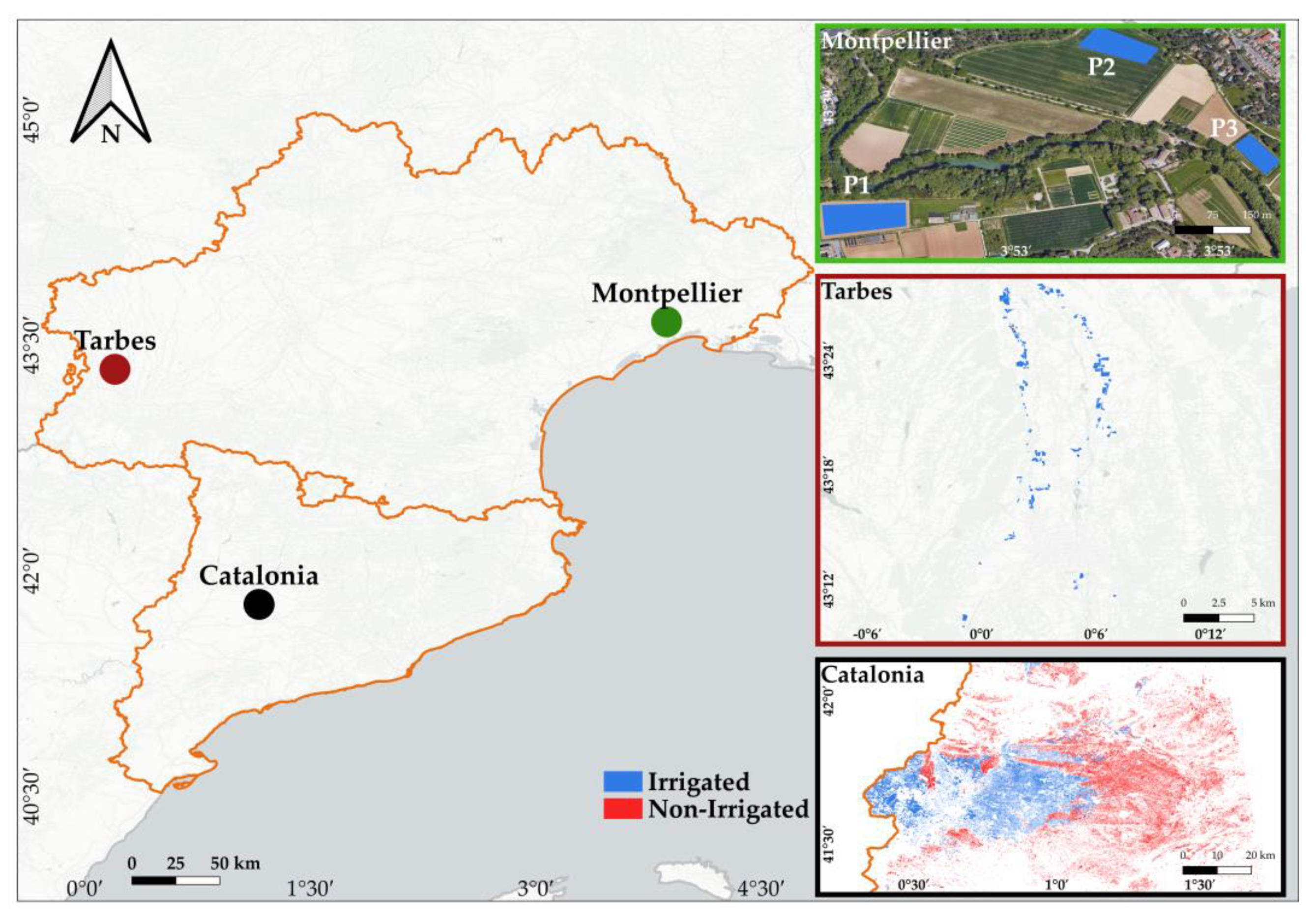
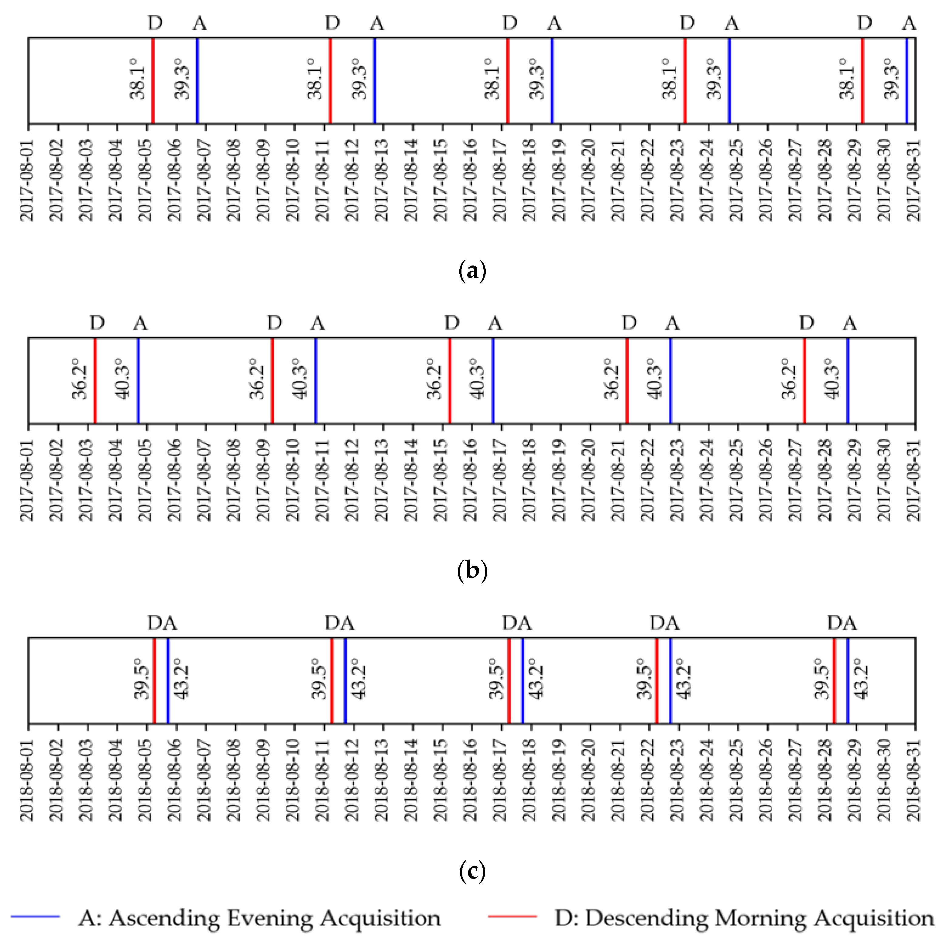
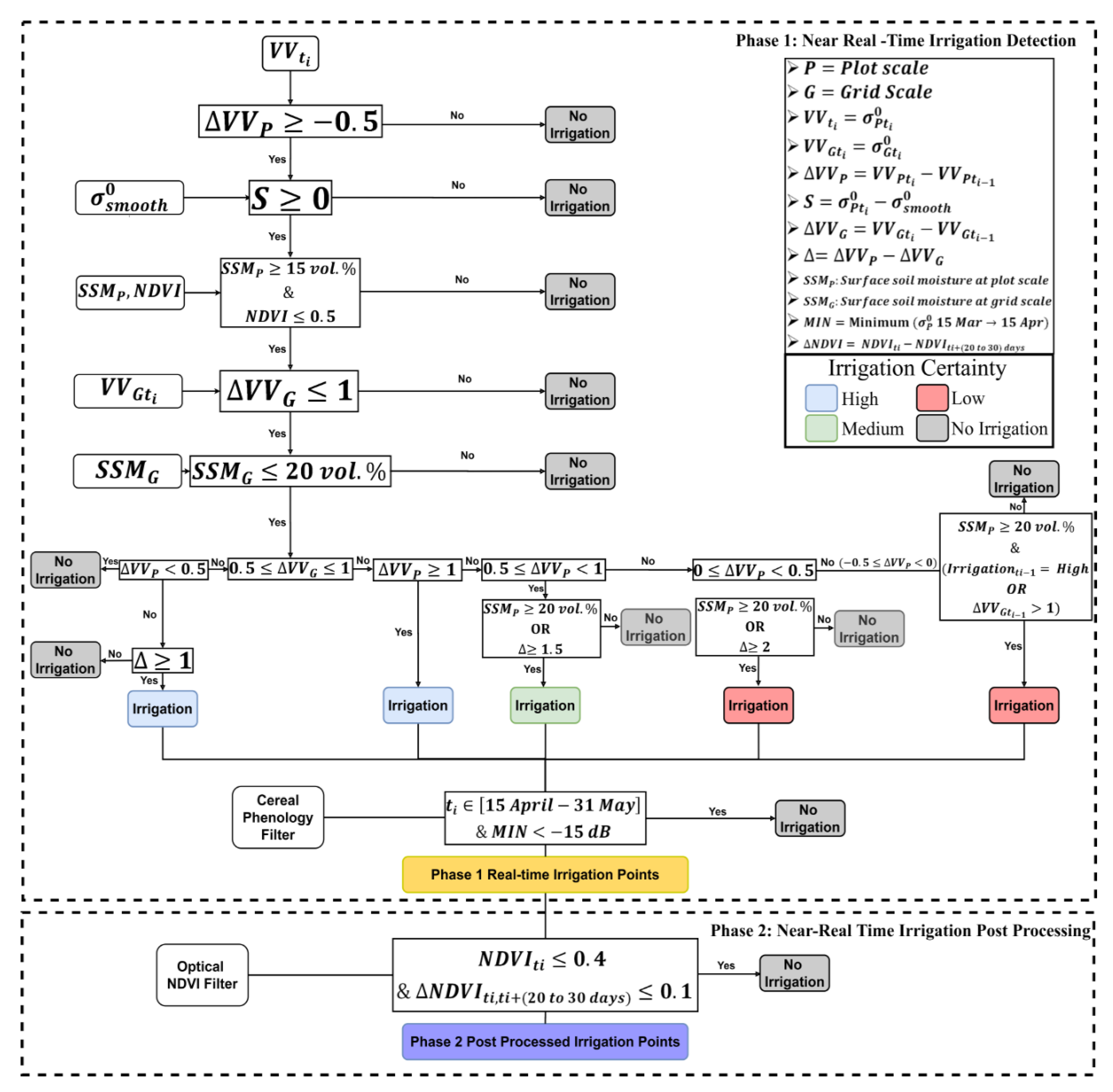
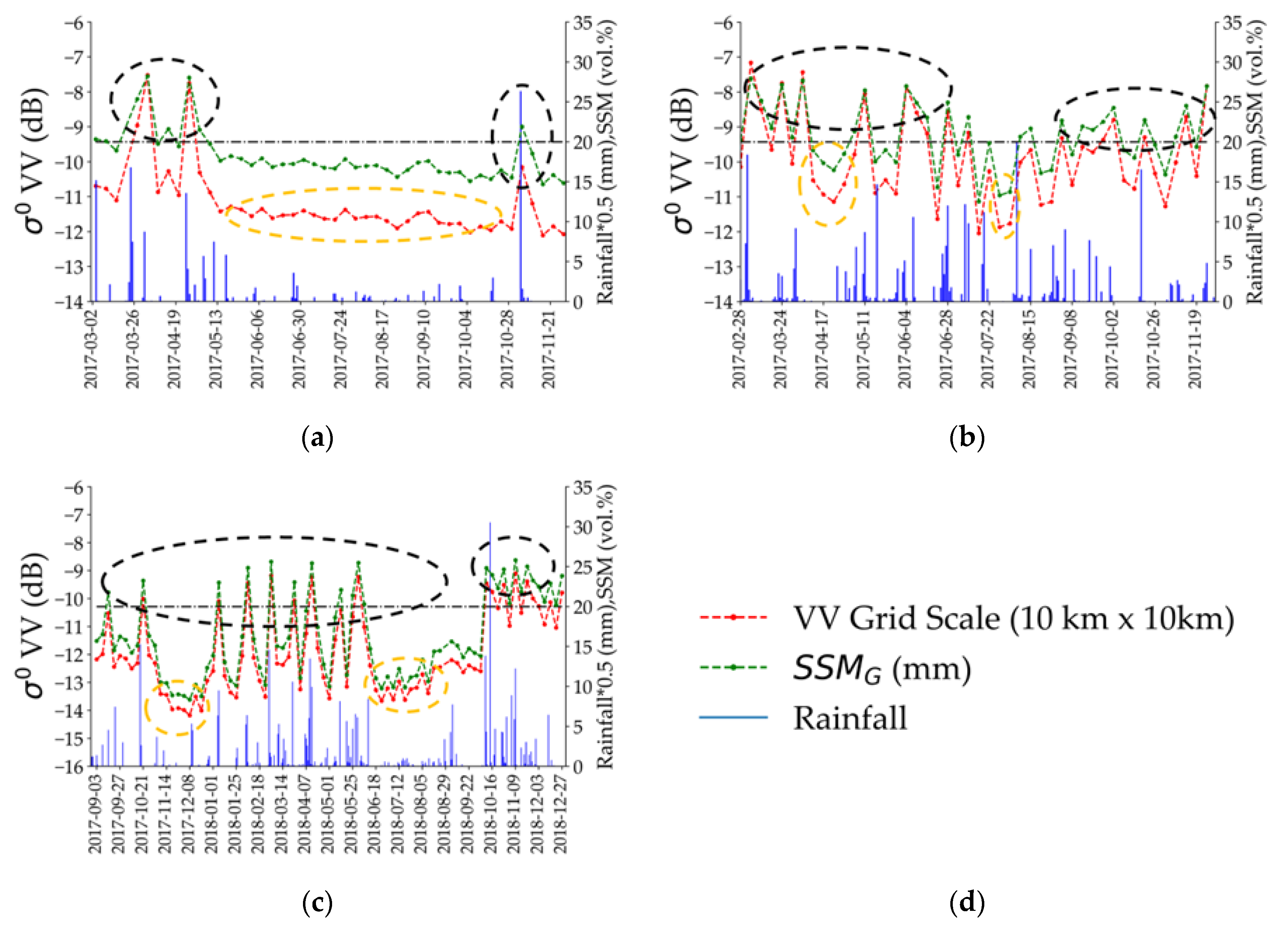
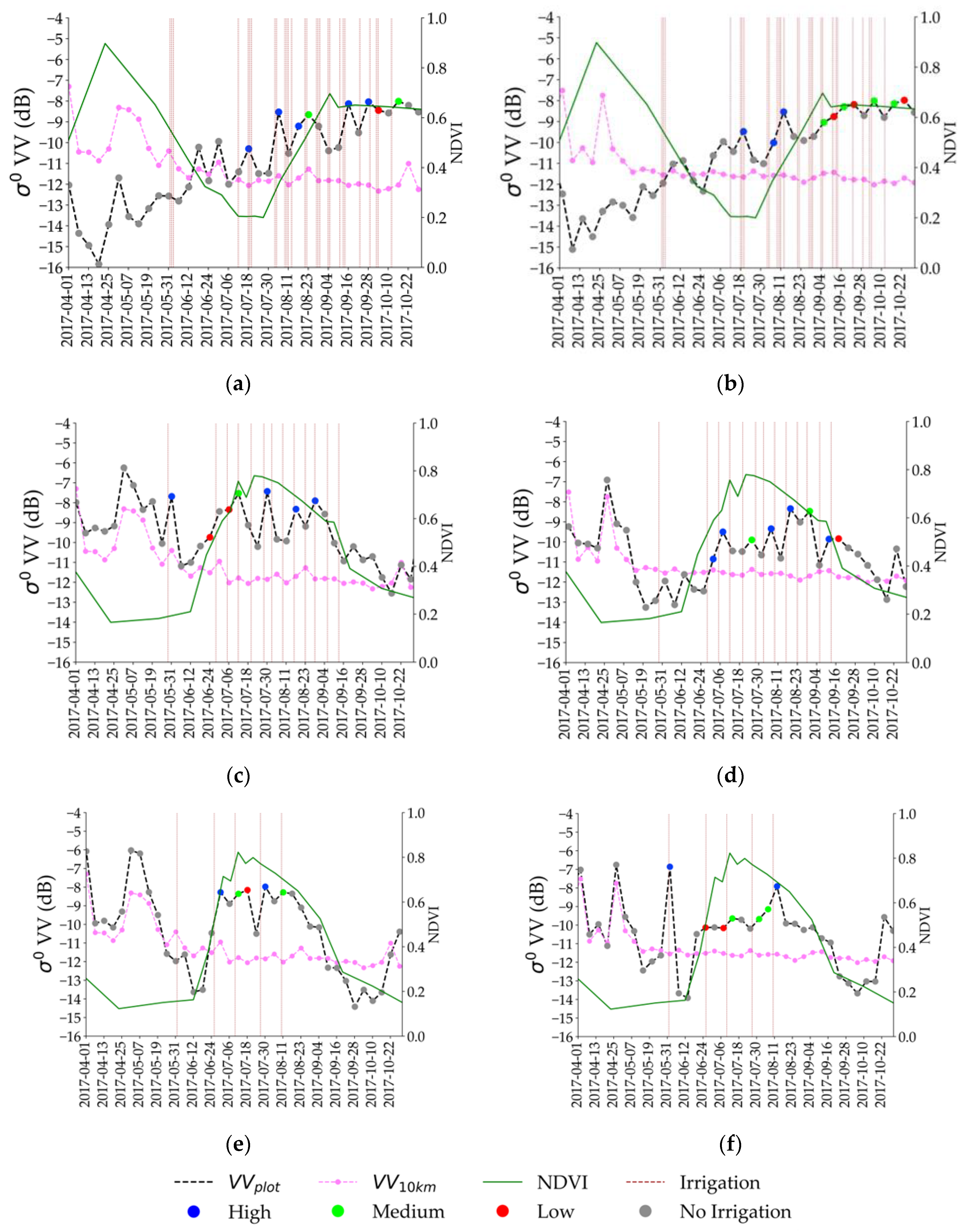
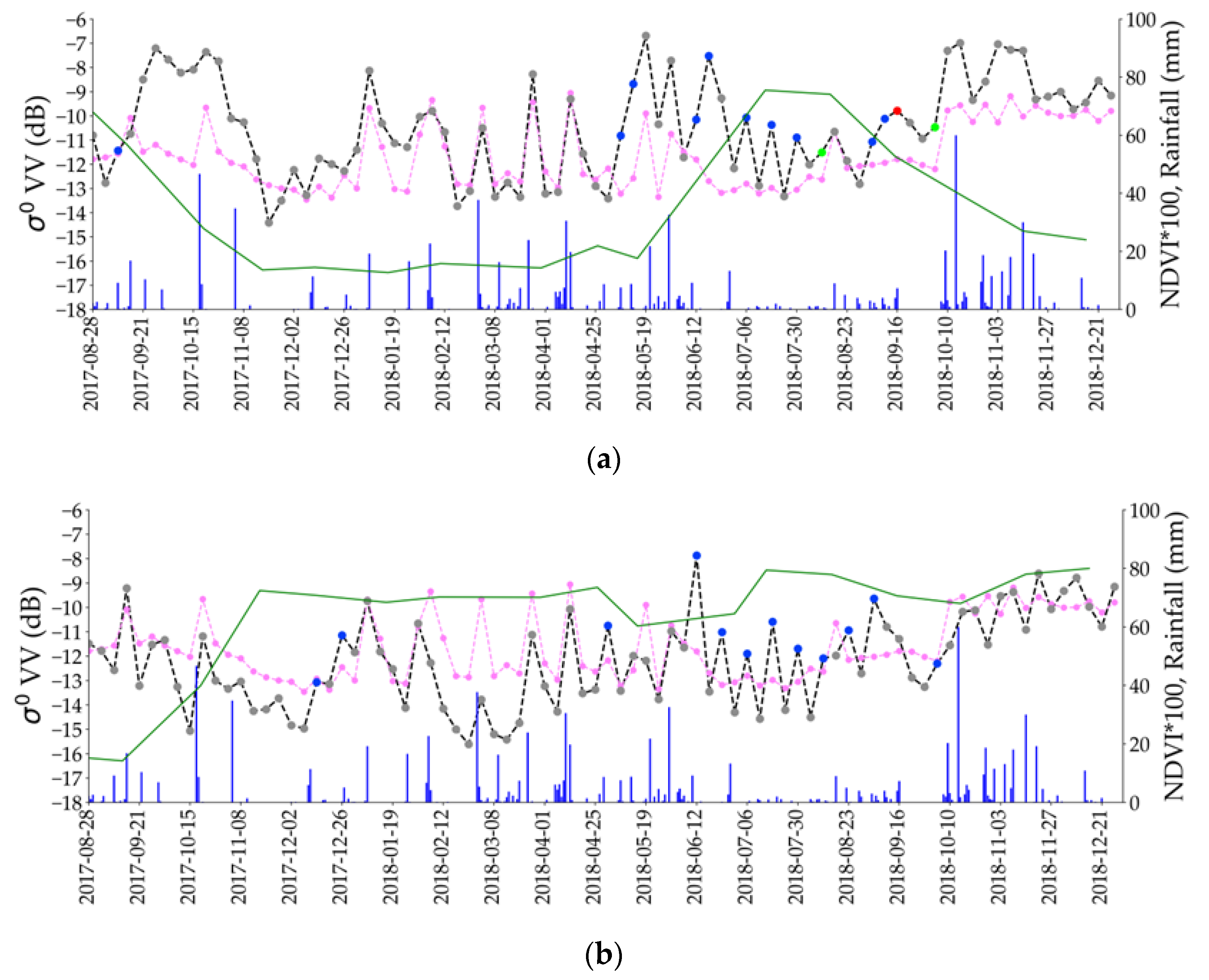
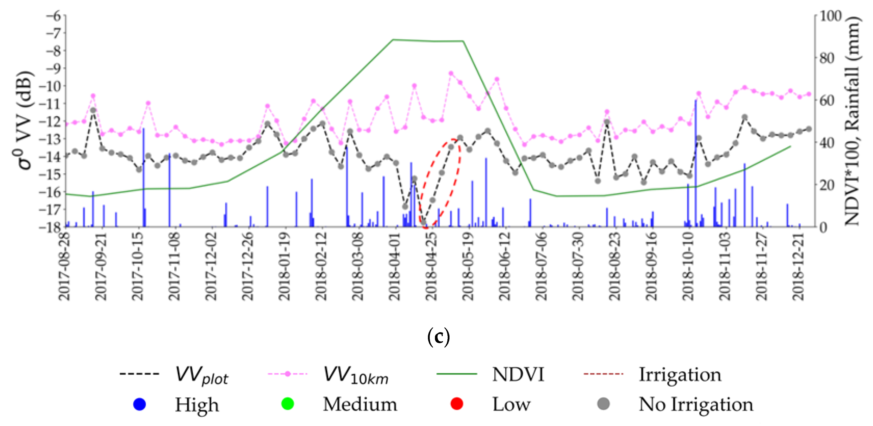
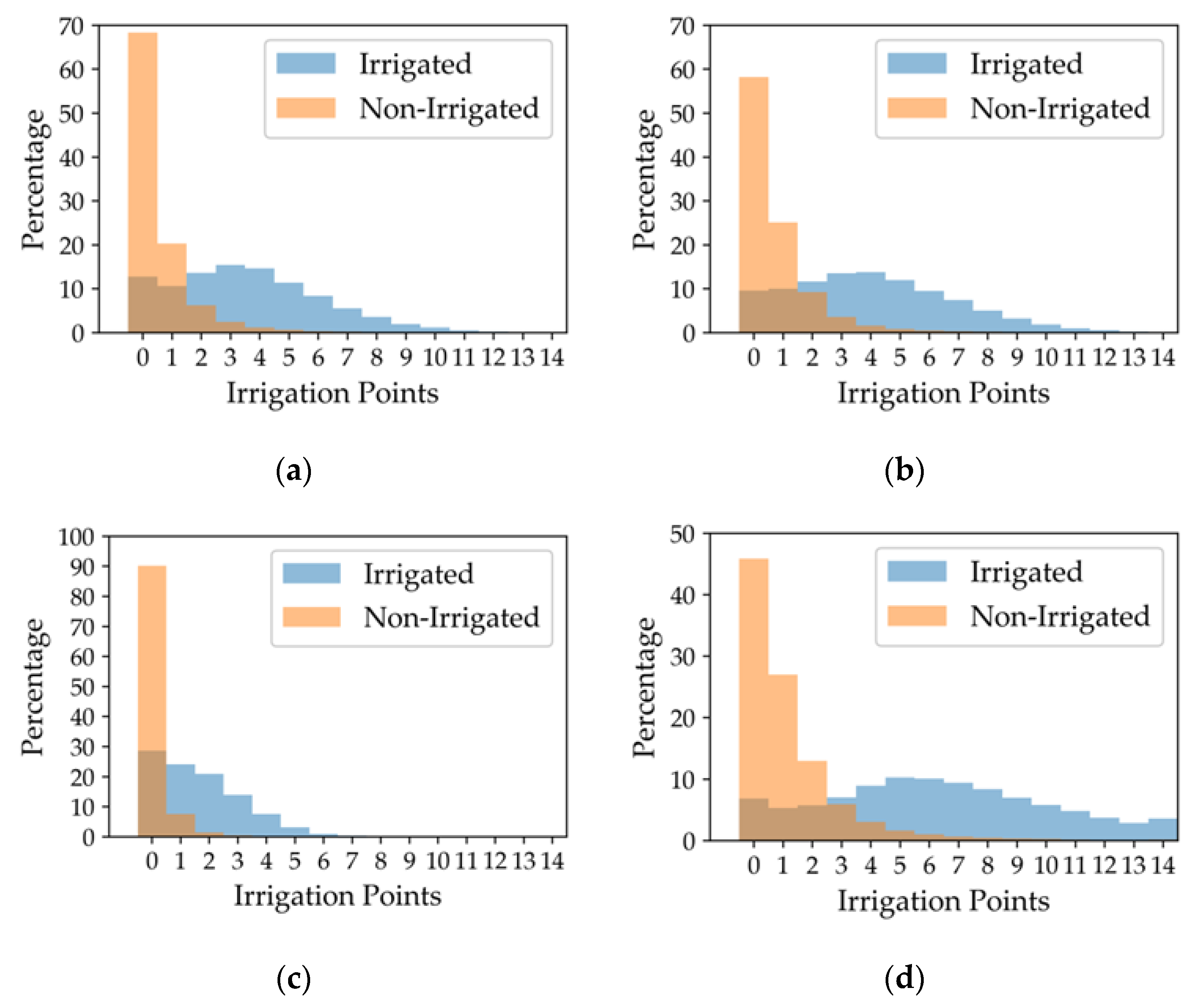
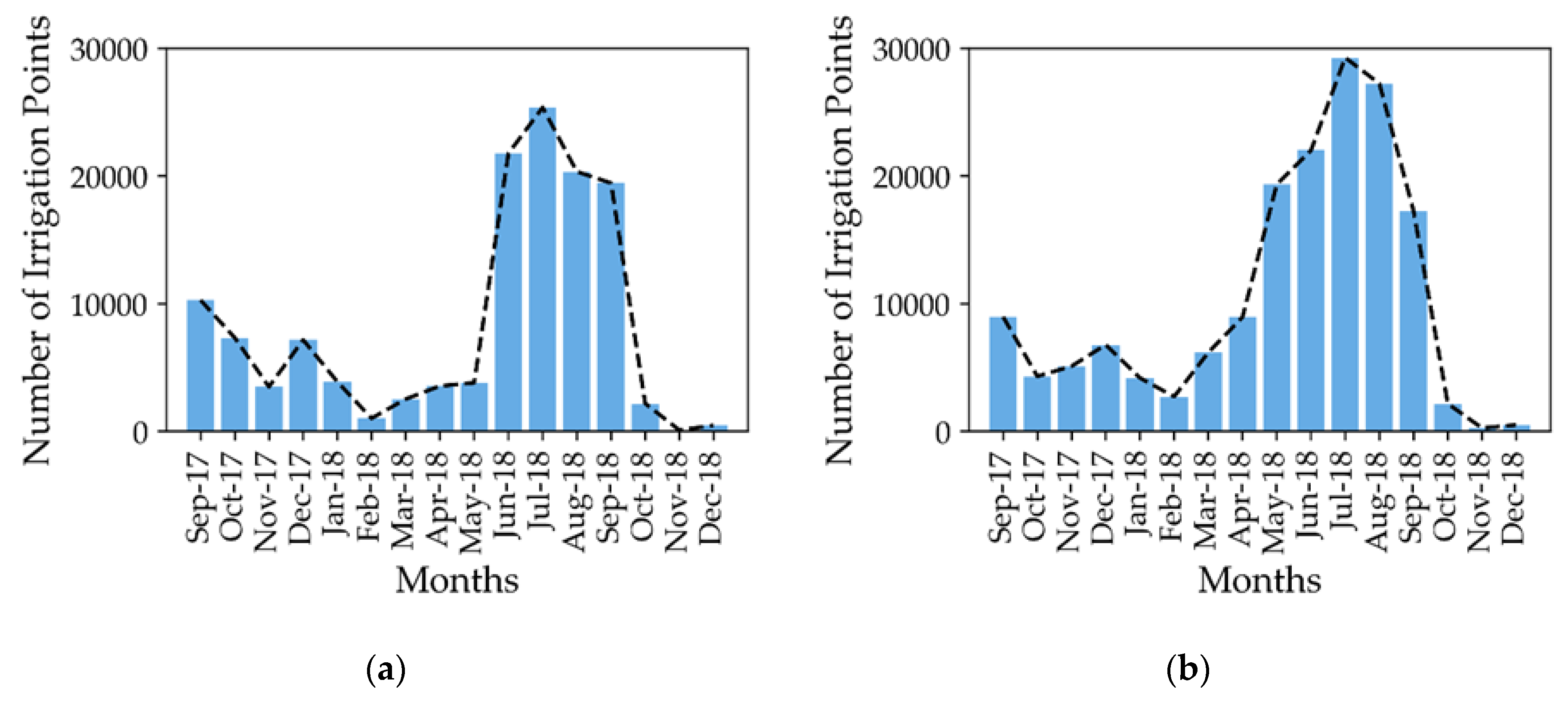
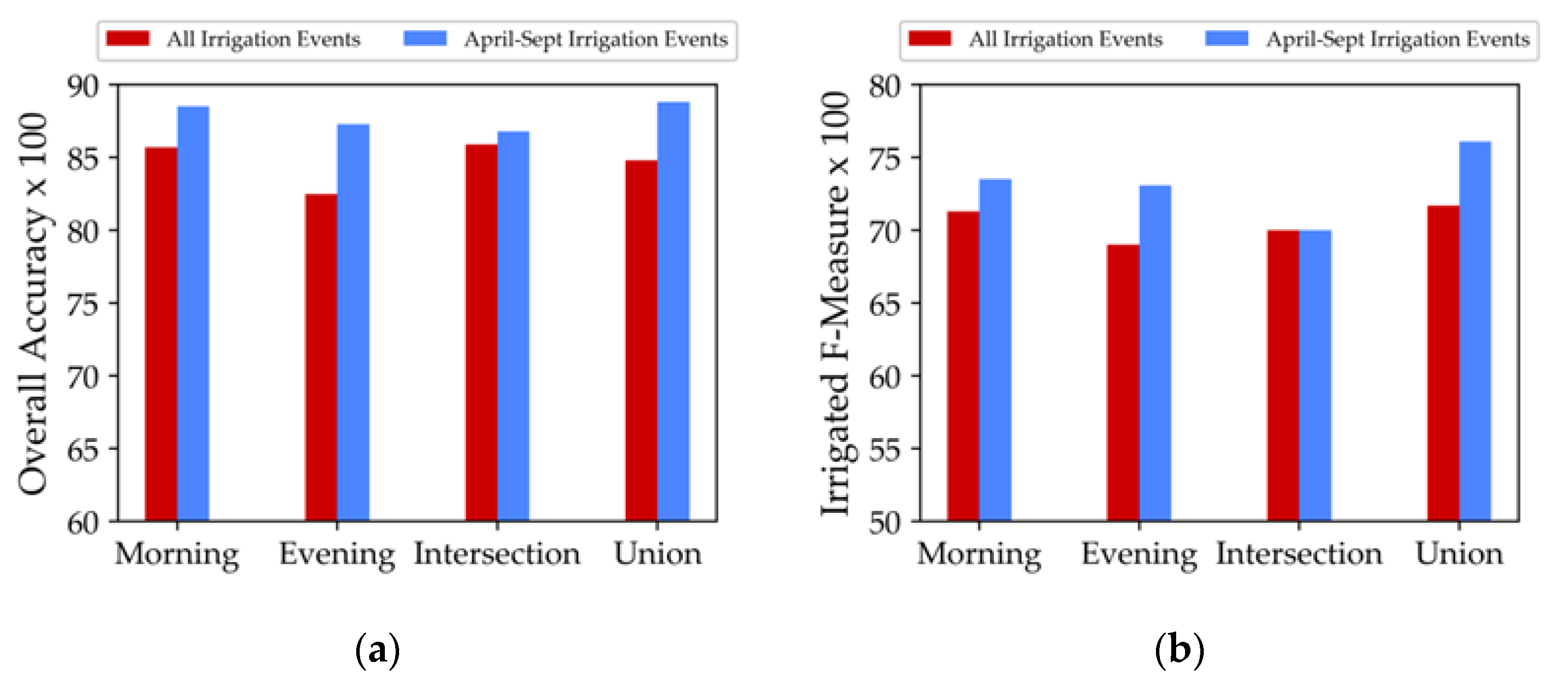
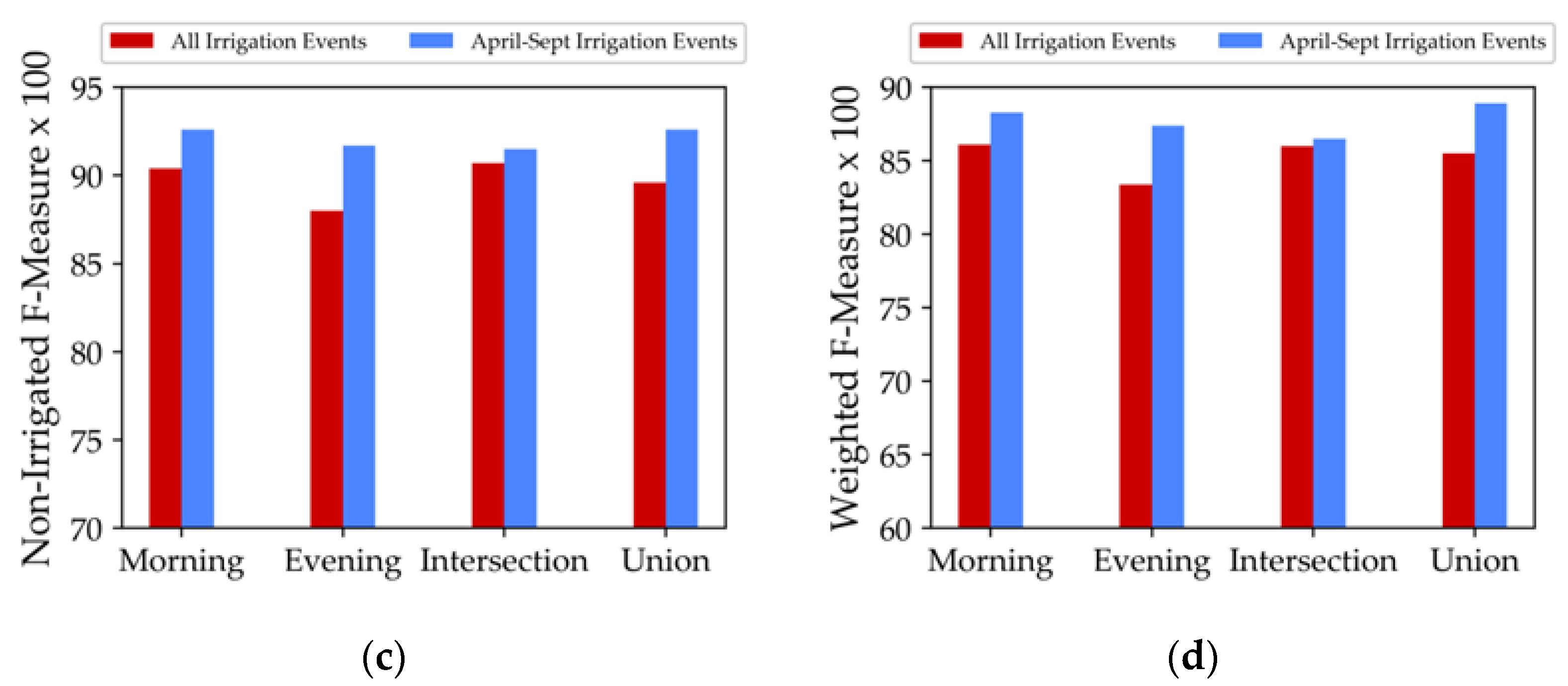
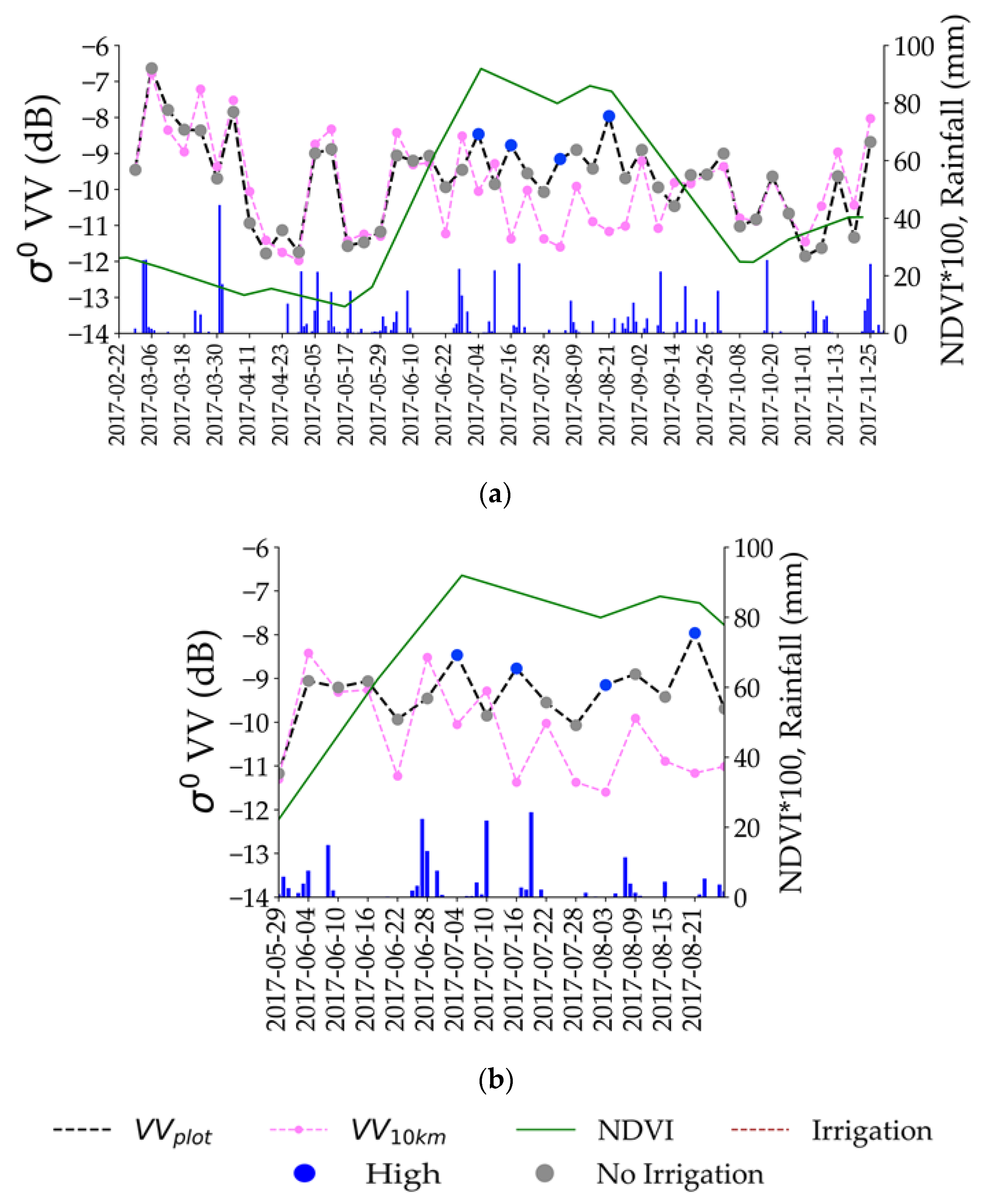
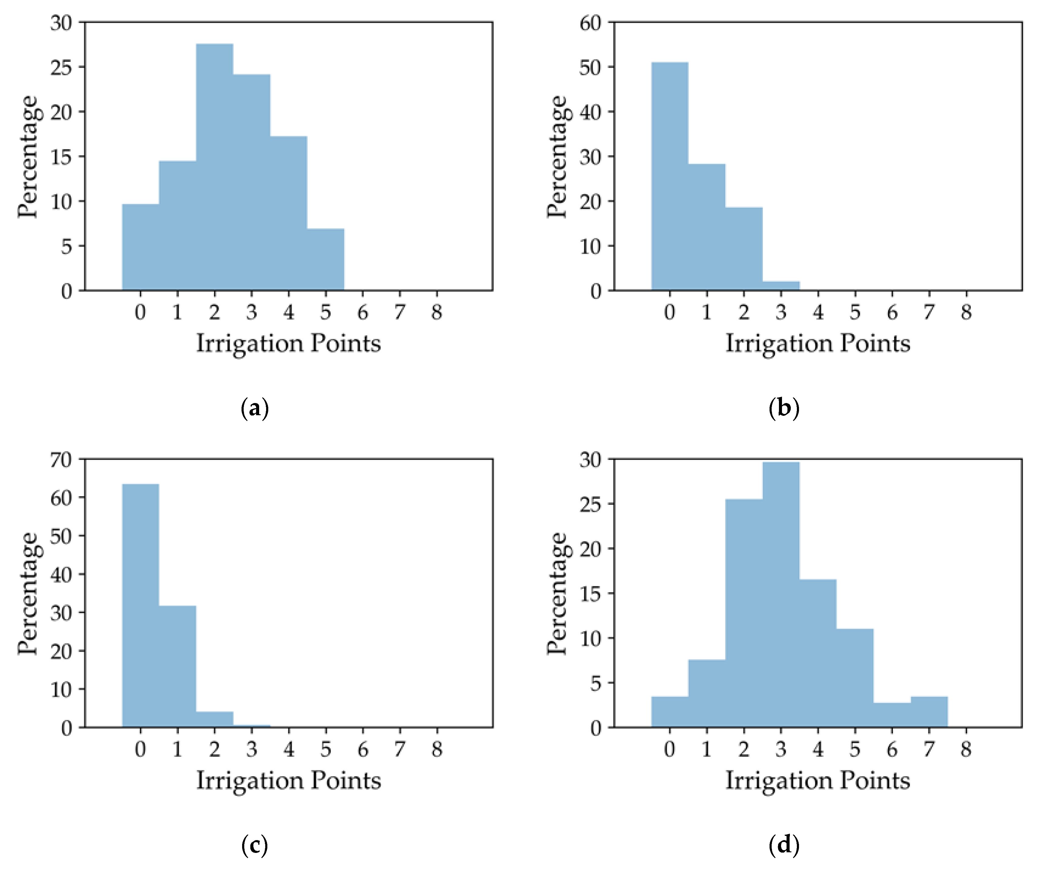
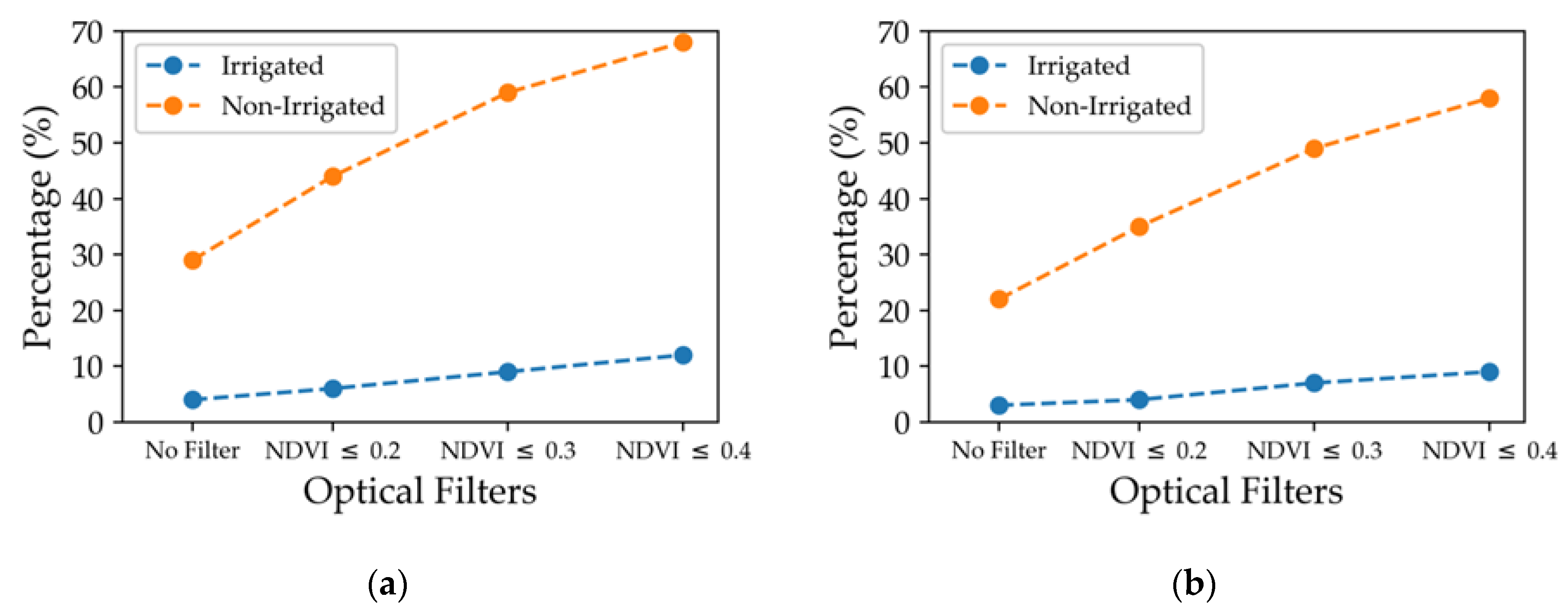
Table 1.
Irrigation information over three plots in Montpellier, south-east France.
| Plot | Crop Type | Surface (ha) | Number of Irrigations | Period of Irrigation | Irrigation Type |
|---|---|---|---|---|---|
| P1 | Maize | 1.2 | 30 | 01 June–12 October 2017 | Sprinkler |
| P2 | Soya | 0.8 | 13 | 29 May–13 September 2017 | Sprinkler |
| P3 | Sorghum | 0.44 | 5 | 01 June–08 August 2017 | Sprinkler |
Table 2.
Irrigation events detected over three plots in Montpellier, South-east France.
| Plot | Number of Irrigation Events | Possibly Detectable Irrigation Events | Detected Irrigation Events | False Detection |
|---|---|---|---|---|
| P1 | 30 | 15 | 12 | 2 |
| P2 | 13 | 13 | 11 | 1 |
| P3 | 5 | 5 | 5 | 2 |
| Total | 48 | 33 | 28 | 5 |
Table 3.
The values of the overall accuracy and F-measure obtained for classification of irrigated and non-irrigated plots using the detected irrigation points for four different scenarios.
Table 3.
The values of the overall accuracy and F-measure obtained for classification of irrigated and non-irrigated plots using the detected irrigation points for four different scenarios.
| Scenario | Condition to be Irrigated | Class | F-Measure | Weighted F-Measure | Overall Accuracy |
|---|---|---|---|---|---|
| SAR Morning | Two points and more | Non-irrigated | 0.90 | 86.1% | 85.7% |
| Irrigated | 0.71 | ||||
| SAR Evening | Two points and more | Non-irrigated | 0.88 | 83.4% | 82.5% |
| Irrigated | 0.68 | ||||
| Intersection Morning and Evening | One point and more | Non-irrigated | 0.90 | 86.0% | 85.9% |
| Irrigated | 0.70 | ||||
| Combined Morning and Evening | Three points and more | Non-irrigated | 0.89 | 84.7% | 85.4% |
| Irrigated | 0.72 |
© 2020 by the authors. Licensee MDPI, Basel, Switzerland. This article is an open access article distributed under the terms and conditions of the Creative Commons Attribution (CC BY) license (http://creativecommons.org/licenses/by/4.0/).
Share and Cite
MDPI and ACS Style
Bazzi, H.; Baghdadi, N.; Fayad, I.; Zribi, M.; Belhouchette, H.; Demarez, V. Near Real-Time Irrigation Detection at Plot Scale Using Sentinel-1 Data. Remote Sens. 2020, 12, 1456. https://doi.org/10.3390/rs12091456
AMA Style
Bazzi H, Baghdadi N, Fayad I, Zribi M, Belhouchette H, Demarez V. Near Real-Time Irrigation Detection at Plot Scale Using Sentinel-1 Data. Remote Sensing. 2020; 12(9):1456. https://doi.org/10.3390/rs12091456
Chicago/Turabian StyleBazzi, Hassan, Nicolas Baghdadi, Ibrahim Fayad, Mehrez Zribi, Hatem Belhouchette, and Valérie Demarez. 2020. "Near Real-Time Irrigation Detection at Plot Scale Using Sentinel-1 Data" Remote Sensing 12, no. 9: 1456. https://doi.org/10.3390/rs12091456
Note that from the first issue of 2016, this journal uses article numbers instead of page numbers. See further details here.