Influence of the Suspended Particulate Matter on the Satellite Radiance in the Sunglint Observation Geometry in Coastal Waters

Abstract

The analysis of satellite ocean color data that are acquired over coastal waters is highly relevant to gain understanding of the functioning of these complex ecosystems. In particular, the estimation of the suspended particulate matter (SPM) concentrations is of great interest for monitoring the coastal dynamics. However, a high number of pixels of satellite images could be affected by the surface-reflected solar radiation, so-called the sunglint. These pixels are either removed from the data processing, which results in a loss of information about the ocean optical properties, or they are subject to the application of glint correction techniques that may contribute to increase the uncertainties in the SPM retrieval. The objective of this study is to demonstrate the high potential of exploiting satellite observations acquired in the sunglint viewing geometry for determining the water leaving radiance for SPM dominated coastal waters. For that purpose, the contribution of the water leaving radiance L_w to the satellite signal L_TOA is quantified for the sunglint observation geometry using forward radiative transfer modelling. Some input parameters of the model were defined using in-situ bio-optical measurements performed in various coastal waters to make the simulations consistent with real-world observations. The results showed that the sunglint radiance is not sufficiently strong to mask the influence of the oceanic radiance at the satellite level, which oceanic radiance remains significant (e.g., 40% at 560 nm for a SPM concentration value of 9 g m⁻³). The influence of the sunglint radiance is even weaker for highly turbid waters and/or for strong wind conditions. In addition, the maximum radiance simulated in the sunglint region for highly turbid waters remains lower than the saturation radiances specified for the current ocean color sensors. The retrieval of L_w and SPM should thus be feasible from radiances measured in the sunglint pattern by satellite sensors, thus increasing the number of exploitable pixels within a satellite image. The results obtained here could be used as a basis for the development of inverse ocean color algorithms that would interestingly use the radiance measured in sunglint observation geometry as it has been done for other topics than the field of ocean color research.

1. Introduction

Satellite observations of ocean color are highly relevant to improve our understanding and monitoring of coastal ecosystems. Such ecosystems are characterized by a considerable spatial variability because of river discharges, wind and tidal/water-level fluctuations. Knowledge of the distribution and transport of suspended particulate matter (SPM) at a synoptic scale is thus of primary importance for investigating the physical and biogeochemical processes occurring in coastal zones. The retrieval of SPM concentrations from satellite remote sensing data first requires the correction of the satellite radiance from the atmospheric effects and from the sea surface effects prior to applying a bio-optical inversion method to convert the derived water leaving radiance, noted L_w, into the SPM concentration. The atmospheric effects include the scattering and absorption processes caused by the presence of molecules and aerosols. The sea surface effects include the direct solar radiance that is specularly reflected from wave facets by the sea surface, so-called the sunglint radiance, and the scattered light that is specularly reflected by the sea surface, so-called the skyglint radiance. The consideration of both the sunglint and skyglint radiances is hereafter referred to as the glint radiance L_glint. The top of atmosphere radiance is referred to as L_TOA.

The analysis of the sunglint radiance measured from satellite data has a considerable potential for various remote sensing applications such as the calibration of satellite bands [1], the estimation of water vapor content [2], the estimation of the absorbing component of aerosols [3], the estimation of the oceanic wind speed [4,5,6,7], the detection of internal waves within the ocean [8], the detection and monitoring of oil spill [9,10], and the estimation of uncertainties in the sea surface temperature retrieval [11]. In the framework of the analysis of ocean color, the sunglint radiance is regarded as a significant nuisance, which seriously limits the ability of determining bio-optical parameters such as the SPM concentration from remotely sensed data. Although the orbit of ocean color sensors is designed to collect most of the data out of the sunglint pattern, a significant amount of pixels within satellite scenes could remain strongly affected by the sunglint radiance, thus leading to an important loss of information. As an example, half of the pixels of an image that was acquired by the Medium Resolution Imaging Spectrometer (MERIS) satellite sensor [12] were contaminated by the sunglint at sub-tropical latitude [13,14]. A few satellite sensors were designed to avoid the sunglint contamination either by tilting from nadir viewing direction as was the case for the Sea-viewing Wide Field-of-view Sensor (SeaWiFS, NASA) instrument [15] and is the case for the current Sentinel3/Ocean and Land Colour Imager (OLCI) instrument (Copernicus, ESA) [16] or by performing multidirectional measurements as was the case for the Polarization and Directionality of the Earth Reflectances (POLDER, CNES) instrument [17]. However, for satellite ocean color sensors that do not have a tilting capability such as the Moderate Resolution Imaging Spectroradiometer (MODIS) instrument [18], many sunglint removal algorithms have been proposed to exploit satellite pixels that are viewed under the sunglint geometry. Kay et al. [19] performed a rigorous review of these various glint correction algorithms. Some of these techniques are based on geometric approaches requiring information on the sea surface state [20,21]; other algorithms are based either on neural networks [22], or on an empirical approach [23] or on polynomial formulations [14]. It should be highlighted that specific methods were developed for correcting high spatial resolution data from the sunglint contamination [24,25,26,27,28].

In open ocean waters, the sunglint signal is much higher than the water leaving radiance in all spectral bands, thus obscuring nearly completely the information of optically active substances carried by the oceanic radiance such as the chlorophyll a pigment concentration (Chl-a). For such a type of waters, there are usually no meaningful retrievals of bio-optical parameters in regions that are significantly contaminated by sunglint unless a glint correction technique is applied [20]. In coastal waters, because the scattering processes induced by the presence of SPM lead to a significant increase of the water leaving radiance, the contribution of L_w to the satellite radiance is strengthened in comparison with both the atmospheric and sunglint radiances. The goal of this study is to investigate the feasibility of detecting SPM concentrations in coastal areas from the top of atmosphere radiance in the sunglint observation geometry when no glint correction techniques are applied. For that purpose, the contribution of the water leaving radiance to the satellite radiance is quantified especially in the sunglint observation geometry for moderately turbid to turbid waters. Forward radiative transfer modelling is used to simulate the various components of the top of atmosphere radiance, namely the water leaving radiance L_w and the glint radiance L_glint. A benchmark case of simulation is analyzed to demonstrate the potential of using the sunglint geometry to determine the water leaving radiance from satellite remote sensing, which has important implications for the derivation of SPM concentrations. The values of the model inputs used for the benchmark case are determined wherever possible from in-situ bio-optical datasets acquired in coastal areas.

The paper is organized as follows. The forward radiative transfer model is described in Section 2 together with the bio-optical datasets that are used to provide the model inputs of the benchmark case of simulation. The angular distribution of the various radiances contributing to the top of atmosphere radiance, namely L_w and L_glint, are analyzed in the principal plane observation geometry (i.e., the plane composed by the specular and backscattering planes) in Section 3. The contribution of L_w to the top of atmosphere radiance L_TOA, which is studied through the ratio L_w/L_TOA, is also examined in Section 3 for the benchmark case with a focus on the sunglint geometry. The sensitivities of such a ratio to the water turbidity, to the wind speed and to the atmospheric turbidity, are discussed in Section 4.

2. Data and Methods

A forward radiative transfer model has been used to simulate the upwelling satellite radiance L_TOA, the water leaving radiance L_w, and the glint radiance L_glint. The model and the datasets used to provide some of the bio-optical input parameters are presented in this section. The benchmark case of simulation is also defined here.

2.1. Radiative Transfer Model OSOAA

The simulations of the various upwelling radiances L_TOA, L_w, and L_glint are carried out using the so-called OSOAA radiative transfer model [29]. The radiative transfer equation is solved by the OSOAA model using the successive orders of scattering method through the atmosphere-ocean system. Such a method allows the multiple scattering effects caused by the water molecules, the hydrosols, the aerosols and the air molecules to be taken into account. The Stokes formalism is used to compute both the radiance and the polarization state of light. The model considers a rough sea surface based on both the Cox and Munk’s [4] wave slope distribution model and the value of the wind speed. The model inputs consist of the bio-optical properties of the hydrosols, namely their scattering and absorption coefficients, and their concentration. The hydrosols are composed of phytoplankton-like particles (e.g., chlorophyll a concentration), mineral-like suspended particulate matter (SPM), and the colored dissolved organic material; the latter is represented by its absorption coefficient (a_CDOM) in the model. The aerosol optical thickness (AOT) and the aerosol optical properties are considered to simulate the atmosphere scattering properties. The model outputs the angular distribution of the radiance and degree of polarization at any altitude or depth for azimuth relative viewing angles φ_OSOAA ranging from 0 to 180° and for viewing zenith angles θ_v ranging from 0° to 70°. It should be highlighted that the geometrical convention that is used by the OSOAA model is defined such that the value of φ_OSOAA of 0° corresponds to an observation made in the Sun specular half-plane (i.e., the Sun and the satellite sensor are in two opposite planes). The specular half-plane is thus the half-plane containing the sunglint reflection. A value of φ_OSOAA of 180° corresponds to an observation made in the anti-specular half-plane (i.e., the Sun and the satellite sensor are located in the same plane), which is in fact the backscattering plane. The so-called principal plane observation is thus defined as the plane composed of these two half-planes (i.e., the values of φ_OSOAA are 0° and 180°). The spectral range of computations allowed by the OSOAA model is the visible/near infrared range from 400 nm to 800 nm. Because the radiances that are initially computed by the OSOAA model are normalized to a value of an extraterrestrial incident solar irradiance E_s of π (unit sr⁻¹ µm⁻¹), the simulated radiances have been multiplied by the ratio E_s/π to account for the sunlight incident illumination, thus providing values of the radiance in geophysical units, namely in W m⁻² sr⁻¹ µm⁻¹. The values of E_s are provided by Thuillier et al. [30]. The reader is referred to Chami et al. [29] for more details about the OSOAA model.

2.2. Data Inputs of the OSOAA Model

A benchmark case of simulation that could be representative of coastal waters is defined. The phase functions of the hydrosols are obtained from Mie theory using values of the refractive index of 1.05 and 1.15 for phytoplankton-like particles and SPM particles, respectively. A Junge power law size distribution, which is characterized by the Junge exponent J, the minimum and maximum radius r_min and r_max, is used for both types of hydrosols. The backscattering ratio, which is defined as the ratio between the particulate backscattering coefficient b_bp and the scattering coefficient b_p, is 0.8% and 2.8% for phytoplankton and SPM particles, respectively. The values of the hydrosol concentrations that are informative of the water turbidity (SPM, chlorophyll a, and a_CDOM at 443 nm) are defined based on in-situ bio-optical datasets to make the simulation close to real-world observations. The SeaWiFS Bio-optical Archive and Storage System (SeaBASS) database (https://seabass.gsfc.nasa.gov/wiki/NOMAD) [31] and the CoastColour Round Robin dataset (CCRR) (https://doi.pangaea.de/10.1594/PANGAEA.841950) [32], which are both publicly available, are used to set the parameters of the water turbidity within the OSOAA model. The use of these databases is relevant for several reasons. First, the data have been collected in various coastal environments at a global scale. The data thus describe the strong variability of the optical properties observed in these dynamic ecosystems. Second, these datasets were primarily designed for performing the validation of remote sensing ocean color algorithms; they are thus composed of high-quality controlled data. Note that because this study is focused on the analysis of coastal waters, only the data collected within 50 km from the coastlines are selected within the SeaBASS and CCRR databases. A statistical analysis of these datasets has been carried out here to compute the median values of the water turbidity parameters that need to be used as inputs of the OSOAA model. Note that the median value is more relevant than the mean value as it minimizes the influence of pronounced regional coastal features. The median values of the Chl-a concentration, SPM concentration, and a_CDOM(443 nm) are 1.8 mg m⁻³, 9.0 g m⁻³ and 0.07 m⁻¹, respectively. The number of data available for which the median was calculated is 366, 38, and 330 for chlorophyll a (Chl-a), SPM, and a_CDOM(443 nm) parameters, respectively. The value of the spectral slope of a_CDOM (S_CDOM), namely 0.0176 m⁻¹, is derived from the analysis performed by Babin et al. [33] in coastal waters. Shettle and Fenn’s coastal model has been used to determine the aerosol optical properties [34]; the value of the aerosol optical depth is set to 0.2, which represents a horizontal visibility of 23 km. The value of the solar incident zenith angle θ_s is 30° and the value of the wind speed is 5 m s⁻¹. The overall input parameters used for the simulation of the benchmark case are summarized in

Table 1. Values of the parameters used for the benchmark case of simulation as inputs of the OSOAA radiative transfer model.

Parameter	Values
Chl-a (mg m−3)	1.8
SPM (g m−3)	9.0
aCDOM(443 nm) (m−1)	0.07
SCDOM (m−1)	0.0176
Refractive index of phytoplankton	1.05 − 0.00i
Refractive index of SPM	1.15 − 0.00i
Junge exponent J (size distribution)	4
Minimum radius (rmin, µm)	0.01
Maximum radius (rmax, µm)	200
Backscattering ratio –phytoplankton (%)	0.8
Backscattering ratio –SPM (%)	2.8
Backscattering ratio of mixed hydrosols (%)	2.5
Aerosol Optical Thickness (AOT)	0.2
Wind speed (m s−1)	5
Solar zenith incident angle θs (°)	30
Seabed depth (m)	50
Seabed composition	Sand

.

2.3. Simulation of the Glint Radiance L_glint and of the Water Leaving Radiance L_w

The OSOAA model is able to simulate the upwelling radiance just above the sea surface (0+). Actually, the radiance calculated at 0+ is the sum of the contribution of the signal exiting the ocean, namely the water leaving radiance L_w, and the atmospheric signal that is reflected by the sea surface, namely the glint radiance L_glint. The glint radiance is thus composed of both the radiance caused by the skylight reflection by the air–water interface (skyglint) and by the incident solar beam reflection by the air-water interface (sunglint). The glint radiance is determined from the radiance at 0+ by performing a specific simulation for which a black ocean is considered (i.e., no scattering processes within the oceanic layer). Note that a specific variable is available within the OSOAA model to remove the scattering processes within the oceanic layer. The water leaving radiance could then be determined by subtracting the glint radiance from the radiance calculated at 0+ when the ocean is no longer black.

3. Results

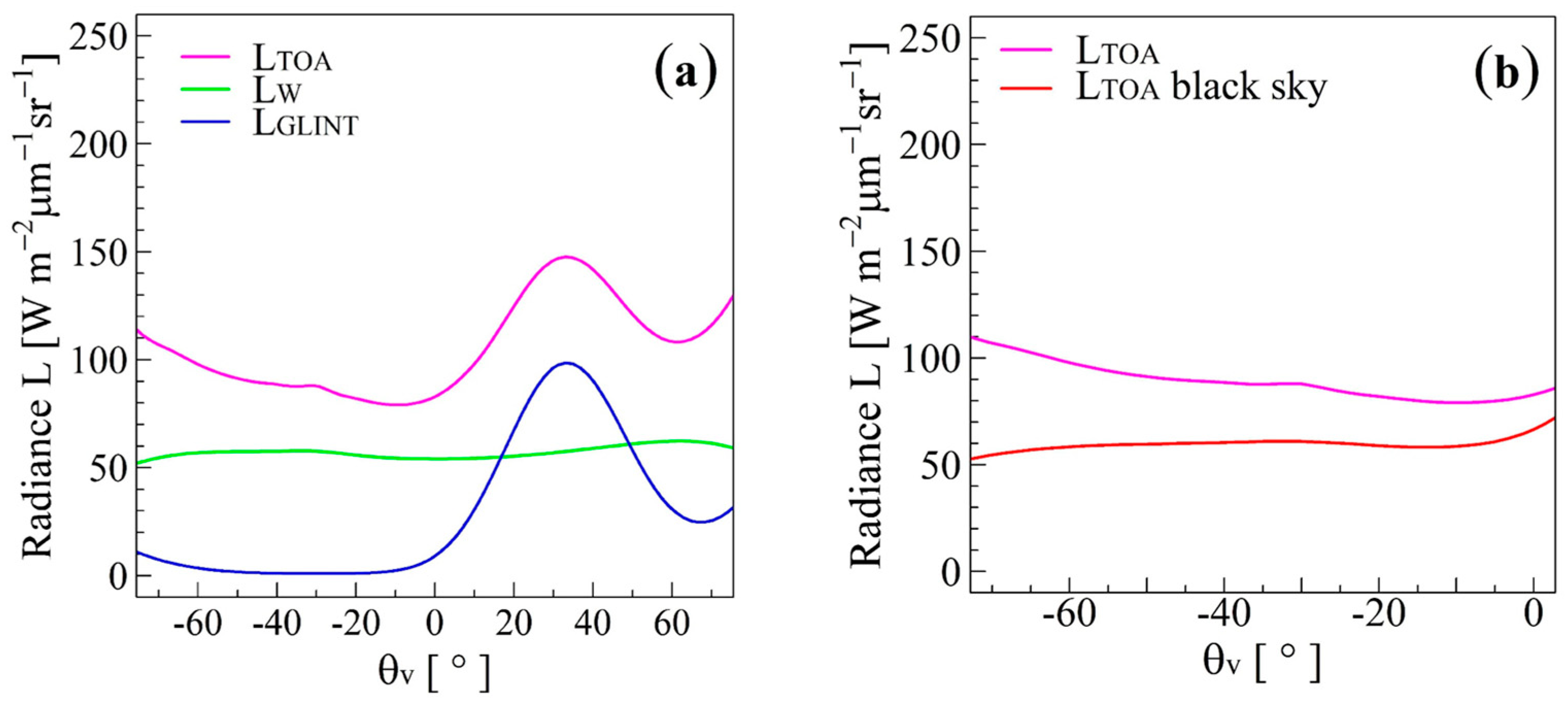
3.1. Angular Variations of the Top of Atmosphere, of the Oceanic and Glint Radiances in the Principal Plane

The angular variations of the top of atmosphere, of the water leaving and glint radiances are examined for the benchmark case of simulation at 560 nm in the principal plane of observation (i.e., φ_OSOAA = 0° and 180°) (Figure 1a).

Figure 1a shows that the glint radiance is highly pronounced around the θ_v value of +30° as expected from the specular reflection of the solar light. The influence of such a specular reflection on the angular distribution of the glint radiance could be observed up to viewing angle values varying within ±20° from the specular direction (θ_v = +30°) as a result of the sea surface roughness induced by the wind. The amplitude of L_glint is negligible in the backscattering half-plane in comparison with the specular plane due to the much lower contribution of the skylight reflection in comparison to the sunlight reflection by the sea surface. The water leaving radiance L_w varies within 20% (i.e., between 50 and 60 W m⁻² µm⁻¹ sr⁻¹) over the entire range of viewing zenith angle in both half-planes. Such an angular variation of the oceanic radiance is consistent with results found in previous studies [35,36,37].

The top of atmosphere radiance L_TOA shows strong angular features. First, a peak of radiance is observed in the specular plane as a direct consequence of the sunglint contribution. Second, L_TOA significantly increases in the backscattering plane, typically by 40% from 80 to 110 W m⁻² µm⁻¹ sr⁻¹ for θ_v values increasing from 0° to −70°. Such a strong angular variation is necessarily due to scattering processes occurring in the atmosphere since both L_glint and L_w do not show such high variations of radiance. To verify that assumption, the top of atmosphere radiance was simulated for the specific case of a black sky condition, which means that all the scattering processes occurring in the atmosphere were removed. The variation of L_TOA for a black sky condition remains fairly flat around 55 W m⁻² µm⁻¹ sr⁻¹ over the range of θ_v [0°; −70°] (Figure 1b). This is because the reflection of the skylight radiation by the sea surface vanishes in the backscattering plane when the scattering by the atmosphere is omitted in the simulation. Therefore, the comparison between the benchmark case and the black sky case of simulations clearly demonstrates the strong influence of the atmospheric scattering in the angular shape of L_TOA in the backscattering plane. More precisely, additional calculations pointed out that the Rayleigh scattering process is the main cause of the observed increase of L_TOA with viewing angle in the backward direction. Chami and McKee [38] previously showed, using in-situ measurements, the strong influence of the skylight reflection by the sea surface on the significant increase of the degree of polarization in the backscattering plane, thus corroborating the major role of the molecular scattering process in the backward increase of the radiance that is observed in Figure 2b.

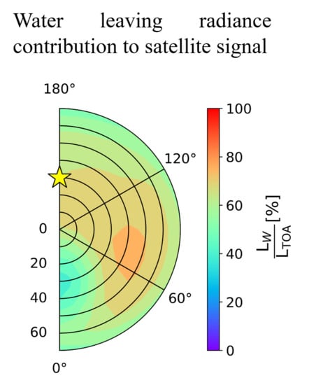
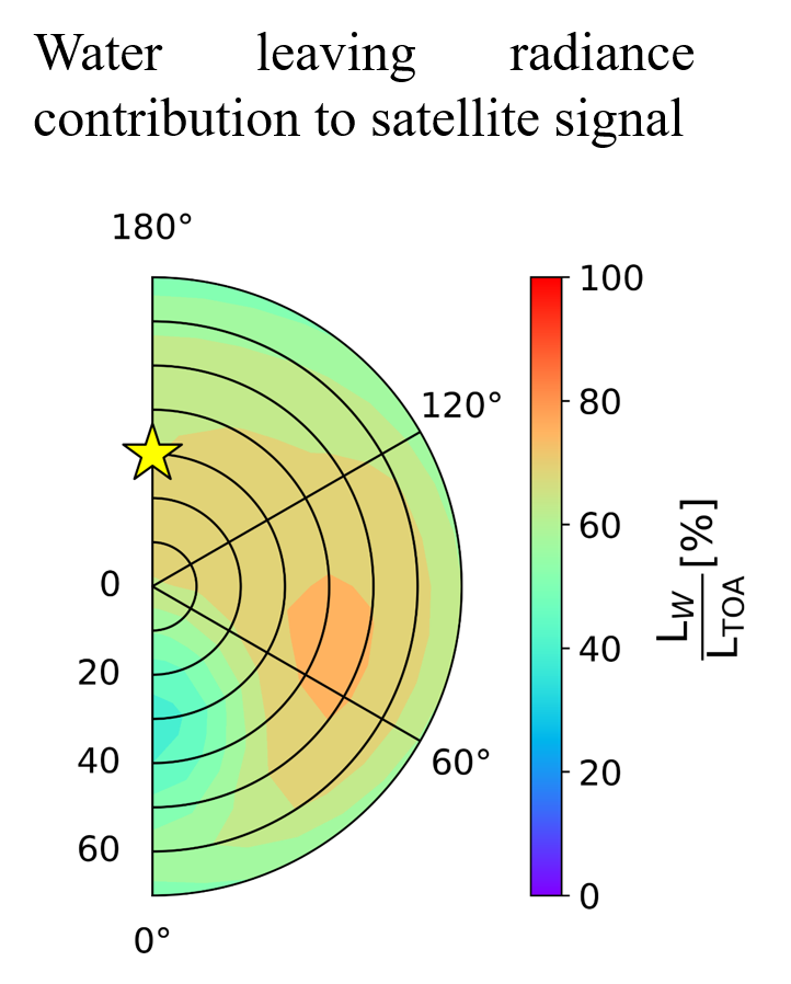
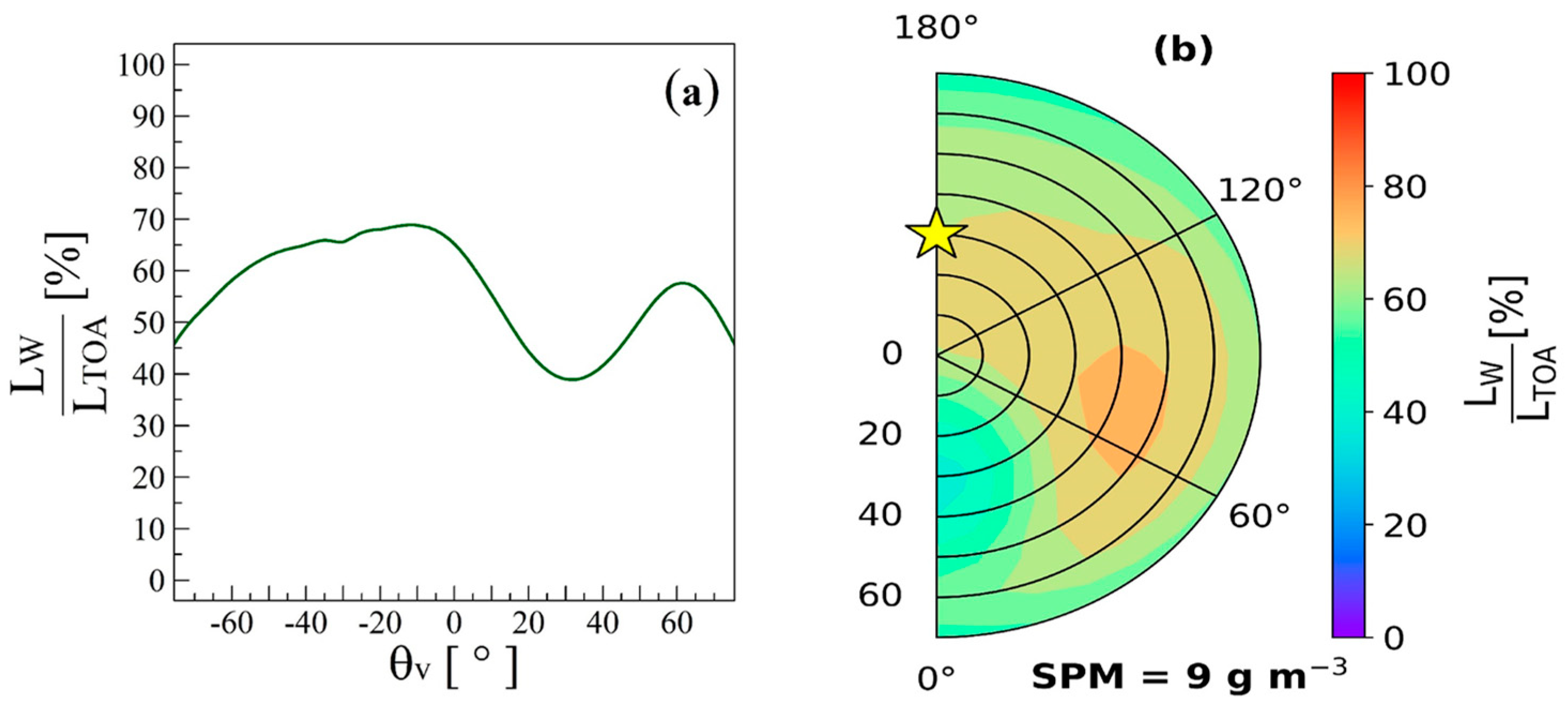
3.2. Angular Variations of the Ratio L_w/L_TOA

The contribution of the water leaving radiance to the satellite radiance could be estimated using the ratio L_w/L_TOA. Figure 2a shows the variation of such a ratio with respect to the viewing zenith angle in the principal plane at 560 nm for the benchmark parameters listed in Table 1. The contribution of the oceanic radiance to the satellite radiance is significant, typically from 40% to almost 70%, with values greater than 50% outside the sunglint geometry. Sturm [39] provided typical values of the contribution of the water leaving radiance to the satellite radiance ranging from 14% to 35% at 550 nm outside the sunglint geometry from clear to turbid phytoplankton dominated waters. It should be highlighted that the values obtained here are based on both an exact forward radiative transfer model and on the use of in-situ bio-optical measurements as inputs of the model while the values provided by Sturm [39] were obtained from the inversion of satellite data. The values found in the current study are higher than those provided by Sturm [39] because of the consideration of mineral-like hydrosols, which are efficient backscatterers (Table 1), in addition to phytoplankton-like hydrosols. Figure 2a thus confirms the well-known potential of using satellite measurements at 560 nm for the retrieval of the SPM concentration in coastal waters out of the sunglint geometry.

For the sunglint observation geometry (around θ_v = +30°), the value of the ratio L_w/L_TOA is expectedly minimal in comparison to other geometries due to the stronger influence of the sunglint radiance (Figure 2a). However, interestingly, the water leaving radiance still contributes by 40% to the top of atmosphere radiance for such a particular geometry. This means that the oceanic radiance is sufficiently high to significantly reduce the influence of the sunglint radiance on the satellite signal. In other words, the sunglint signal does not totally obscure the information provided by the SPM contained in L_w. Yet, sunglint effects have systematically been considered as a serious limitation for accurately determining water optical characteristics from remotely sensed ocean color data (Section 1). The results shown here indicate the feasibility of using the satellite radiance measured in the sunglint geometry for determining the water leaving radiance in the case of moderately turbid waters. Note that the values of the ratio L_w/L_TOA remain significant at 560 nm whatever the azimuth and viewing zenith angle outside the principal plane (Figure 2b). A maximum value of 80% is reached for a geometry that is far from the sunglint pattern, namely a relative azimuth angle value φ_OSOAA of 70° and a viewing zenith angle of 45°, which could be an optimized geometry for the retrieval of water leaving radiance from satellite data for the treated case of simulation.

4. Discussion

The simulations performed in this study depend on the phase functions that were calculated using Mie theory for two types of hydrosols, namely phytoplankton and mineral-like particles (Table 1). The modelled phase functions (Figure 3) are quite consistent in their general shape with many observations acquired over a broad range of oceanic water types, especially their backward portion (i.e., from 90° to 180°) [40,41,42,43]. Note that the backward portion of the phase function is of major interest for the purpose of satellite remote sensing. In particular, the particulate backscattering ratio is a key parameter that enables the influence of mineral-like hydrosols (SPM) on the water leaving and satellite radiances compared to the influence of biogenic particles to be highlighted. The theoretical values calculated here for both types of hydrosols (Table 1) are consistent with those measured by Sullivan et al. [44] in a SPM-dominated water type (Santa Barbara channel, USA) and in a phytoplankton-dominated water type (Monterey Bay, USA), respectively. Note, however, that a strong variability in the backscattering ratios is often observed in natural waters. As an example, Twardowski et al. [42] measured values ranging from 3.9% to 7.8% in waters characterized by turbid patches of resuspended sediment in the site of Scripps Pier (La Jolla, USA). Zhang et al. [43] observed a biogenic backscattering ratio of 0.16% in the site of Monterey Bay while Sullivan et al. [44] measured higher ratios ranging from 0.5% to 1.5% for the same phytoplankton-dominated study area. Zhang et al. [43] recently examined the partition of the measured phase function into two components due to particulate organic matter and particulate inorganic matter. Their analysis revealed that the fractional contribution by mineral-like particles to the backward portion of the phase function significantly increases with scattering angles from 60% to almost 90% for the case of a SPM-dominated water type in the Gulf of Mexico (Mobile Bay, USA). Therefore, a backscattering efficiency of SPM higher by about 3.5 times than phytoplankton’s one, as modeled in the current study (Table 1), is consistent with Zhang et al. findings [43]. Thus, the theoretical phase functions and backscattering ratios used here for the simulations are in agreement with observations performed in various SPM-dominated coastal waters.

As mentioned in Section 3, the angular variation of the satellite radiance with respect to the viewing zenith angle in the principal plane of observation is characterized by two main features, which are the strong influence of the sunglint radiance in the specular plane and the significant influence of the skylight reflection by the sea surface in backscattering plane. However, despite the amplitude of these effects, the water leaving radiance remains a significant contribution of the top of atmosphere radiance from 40% to 70%, including within the sunglint pattern. The contribution of L_w to L_TOA could even reach 80% out of the principal plane geometry. The range of variation of the ratio L_w/L_TOA is much greater than the range observed by SeaWiFS (NASA) satellite sensor over the global ocean, which is typically between 5% and 20% [45]. Higher values of L_w/L_TOA are expected here as a result of the strong scattering induced by the presence of SPM in coastal turbid waters.

Although the correlation between the SPM concentration and the water leaving radiance is high in green wavelengths such as 560 nm, the choice of using radiances measured in red wavelengths, typically between 600 nm to 670 nm, is often made to derive SPM concentrations from remotely sensed data [46,47,48,49,50,51]. This is because of the potential saturation of the water leaving radiance with SPM concentrations in green bands that is commonly observed in turbid waters [47]. Therefore, the angular variation of the ratio L_w/L_TOA has been examined at 620 nm and for various oceanic turbidities, namely for SPM concentrations of 1, 9, and 70 g m⁻³ (Figure 4).

The overall contribution of L_w to L_TOA is lower at 620 nm (Figure 4) than that observed at 560 nm (Figure 2) as a consequence of the increased absorption by the water molecules in the red, thus reducing the amount of the signal exiting the ocean. As an example, L_w contributes to L_TOA between 10% and 50% for the SPM value of 9 g m⁻³ compared to the range of 40% to 80% previously observed at 560 nm (Figure 2b). The minimum value of the ratio is systematically observed for the sunglint observation geometry whatever the turbidity. This is because of the higher influence of the sunglint radiance for such geometry, thus leading to a relative decrease contribution of L_w to L_TOA.

The influence of the water turbidity on the ratio L_w/L_TOA clearly shows that the oceanic radiance contribution to L_TOA is too weak in clear waters (Figure 4a), typically less than 10%, especially in the sunglint region, to be able to properly exploit the satellite radiance in the red band for retrieving the optical signature of the hydrosols for the sunglint geometry. However, the red band appears to be relevant to exploit the water leaving radiance from satellite data in highly turbid waters for which the ratio L_w/L_TOA varies from 50% to 90% over all the geometries (Figure 4c). In particular, satellite observations performed in the sunglint geometry remain highly relevant for detecting SPM using red bands. One advantage of using both green and red spectral bands is that band ratio algorithms have been shown to be effective to retrieve the SPM concentrations in coastal turbid waters [46,47,50,51].

Additional radiative transfer simulations were carried out based on Table 1 to calculate the maximum radiance L_max that could be measured over all the geometries at the top of atmosphere for highly turbid waters, namely a value of SPM of 70 g m⁻³. The values of L_max are 251 W m⁻² µm⁻¹ sr⁻¹ and 176 W m⁻² µm⁻¹ sr⁻¹ at 560 nm and 620 nm, respectively. As a comparison, the saturation radiances of the Sentinel 3/OLCI (Copernicus/ESA) satellite sensor are 525 W m⁻² µm⁻¹ sr⁻¹ and 398 W m⁻² µm⁻¹ sr⁻¹ at 560 nm and 620 nm, respectively [16]. The saturation radiances of the VIIRS (NASA/NOAA) satellite sensor are 667 W m⁻² µm⁻¹ sr⁻¹ and 718 W m⁻² µm⁻¹ sr⁻¹ at 555 nm and 640 nm, respectively [52]. Therefore, the sum of the sunglint and the water leaving radiances should not lead to saturate satellite pixels of the current satellite ocean color sensors, thus confirming the feasibility of using satellite radiances measured in the sunglint geometry for retrieving the SPM concentrations for moderately turbid to turbid waters (i.e., SPM values greater than 9 g m⁻³).

Since the sea surface roughness is mostly driven by the wind strength, the sensitivity of the ratio of L_w/L_TOA to the wind speed WS (in m s⁻¹) is examined for the specular direction (θ_v = +30°, φ_OSOAA = 0°) (Figure 5). For that purpose, the simulations are performed using the input parameters listed in Table 1 but for wind speed values varying from 1 m s⁻¹ to 15 m s⁻¹, namely 1, 5, 10, and 15 m s⁻¹. Results are shown at 560 nm (Figure 5a) and 620 nm (Figure 5b) for various SPM concentrations, namely 1, 9, and 70 g m⁻³.

The ratio L_w/L_TOA significantly increases with higher wind speed values. As an example, the ratio increases by a factor of 2.7 at 560 nm (Figure 5a) and by a factor of 4 at 620 nm (Figure 5b) when the wind speed increases from 1 to 15 m s⁻¹ for a SPM value of 9 g m⁻³; the increase is especially sharp from 1 to 5 m s⁻¹ with a factor of 2. Such a shape of variation could be explained by the fact that the extent of the sunglint is controlled by the distribution of wave slopes on the sea surface, which is linearly related to wind speed as modelled by Cox and Munk [4]. The sunglint pattern is thus more spatially widened as the wind speed increases. For strong wind speed values, typically greater than 5 m s⁻¹, the amplitude of the surface reflected solar radiation is significantly reduced in the sole specular direction (θ_v = +30° here) due to the higher variance of the wave slope distribution. Therefore, the sunglint radiance is weaker in that specular direction, which enables the water leaving radiance to be more easily distinguished at the top of atmosphere level. In addition, Koepke [53] showed that the contribution of whitecaps is small even for wind speed as high as 15 m s⁻¹. These results thus confirm the high potential of satellite remote sensing data acquired in the sunglint geometry for determining the SPM concentrations from the water leaving radiance in the coastal ocean. However, it should be highlighted that such an approach would not be applicable for clear waters (e.g., SPM = 1 g m⁻³) and for a nearly flat ocean surface (WS= 1 m s⁻¹) where the contribution of L_w to L_TOA is lower than 10% (Figure 5). In the case of clear waters, this is because of the weak influence of the scattering processes in the water column; in the case of a nearly flat ocean, this is because of the major influence of the sunglint radiance that masks the ocean optical signature. Conversely, an approach which would consist in exploiting the satellite radiance measured in green and red spectral bands in the sunglint observation geometry for deriving the SPM concentrations would be the most useful for moderately turbid to turbid waters, typically for SPM values greater than 9 g m⁻³, and for moderate to strong sea surface roughness, typically for wind speed values greater than 3 m s⁻¹. Note that Harmel and Chami [54] showed based on the analysis of satellite data that the wind speed values mostly vary from 4 m s⁻¹ to 7 m s⁻¹ over the entire globe.

Finally, the sensitivity of the ratio L_w/L_TOA to the atmospheric turbidity, namely the aerosol optical depth AOT, has been examined in the specular direction for the input parameters listed in Table 1 and for values of AOT of 0.1, 0.2, and 0.5 (Figure 6). The ratio regularly increases with the atmospheric turbidity. This is due to a decrease of L_TOA in the specular direction resulting from the weaker direct atmospheric transmittance when AOT is higher. In any case, the atmospheric turbidity does not alter the main conclusions previously drawn about the potential of deriving the water leaving radiance in the sunglint observation geometry.

5. Conclusions

The satellite remote sensing of coastal waters is of great interest for improving our understanding of the functioning of these dynamic ecosystems. It is also of particular importance for a variety of applications dedicated to coastal management which often implicitly contain an economic interest. The top of atmosphere radiance L_TOA is composed of the water leaving radiance L_w, the atmospheric radiance and the glint radiance L_glint; the latter includes both the components of the skylight and the sunlight reflections by the sea surface. The retrieval of bio-optical parameters such as the chlorophyll a concentration or the suspended particulate matter (SPM) concentrations from ocean color satellite data is commonly performed for pixels that are not contaminated by the sunglint pattern, which is mainly located near the specular direction in the principal plane (i.e., the plane that contains both the sun and the satellite sensor). This is because the sunglint radiance is often so high that it could mask the information provided by the water leaving radiance, especially in the open ocean or weakly turbid waters. In this study, the potential of using the satellite radiance measured in the sunglint geometry for the retrieval of L_w and its implications for deriving the SPM concentrations in coastal waters has been investigated based on forward radiative transfer modelling. A benchmark case of simulation was defined. The model input parameters were set based on bio-optical in-situ datasets that were acquired in various coastal areas, thus making the simulations consistent with real-world conditions. In particular, the median values of the concentrations of the hydrosols were used to account for the strong variability of the hydrosols encountered in coastal zones. Note also that the modelled phase functions and backscattering efficiencies of SPM and phytoplankton hydrosols were consistent with observations.

First, the angular distribution of the different radiance components which compose the satellite signal, namely L_TOA, L_w, and L_glint, was analyzed in the principal plane of observation. The glint radiance L_glint showed a pronounced peak in the specular plane, as a result of the surface specularly-reflected solar radiation. The water leaving radiance L_w varied within 20% over all the viewing directions; such a directional variation was consistent with results found in previous studies. The top of atmosphere radiance showed a significant increase by up to 40% with viewing zenith angles in the backscattering plane. The increase was explained by the importance of the skylight reflection by the sea surface originating from the Rayleigh scattering process. Such a result could be further used to help the interpretation of the satellite directional radiance that will be measured in the near future by forthcoming multidirectional satellite sensors such as the Multidirectional, Multipolarization and Multispectral (3MI) instrument (ESA and EUMETSAT) and, to a lesser extent, the Ocean Color Instrument (OCI) NASA) which should be able to acquire directional measurements thanks to polarimeters in the frame of the PACE mission (NASA).

Second, the contribution of the water leaving radiance to the satellite signal was analyzed through the ratio L_w/L_TOA. The results revealed that such a contribution is significant, typically between 40% and 80% at 560 nm for turbid waters over all the observation geometries. It was noted that this range of variation is much lower for open ocean waters. Our results thus demonstrated that the optical signature of L_w should not be masked by the sunglint radiance at the satellite level when observing waters showing a turbidity greater than 9 g m⁻³. The sensitivity analysis that was carried out showed that measurements performed in the sunglint geometry using a red spectral band is also suitable to derive SPM concentrations provided that turbid waters are concerned. It was also shown that the detection of SPM using the radiance measured in the specular direction is even more feasible when the sea surface is strongly agitated due to the higher spatial extent of the sunglint pattern. In addition, it was mentioned that the maximum radiance that is expected at the top of atmosphere in turbid waters within the sunglint region remains lower than the saturation radiance of the current ocean color sensor, thus making it possible to measure it. The improvement of the radiometric saturation specifications of the current satellite instruments is therefore not necessary. This study also revealed that the observation of the ocean color in the specular direction should not be helpful for clear waters and/or for a nearly flat ocean surface because the water leaving radiance is either not sufficiently high (clear waters) or masked by the sunglint radiance at the satellite level (flat surface). It was also noted that the atmospheric turbidity does not change the conclusions drawn in this study.

The results presented in this paper could be then used as a basis for the development of inverse algorithms dedicated to the retrieval of SPM in turbid coastal waters from the use of satellite data acquired in the sunglint geometry. The sunglint radiance could thus be treated as relevant information, as it was previously exploited for other topics (Section 1), rather than a nuisance information for ocean color. Inverse algorithms based on the exploitation of the sunglint radiative properties would extend the analysis of a given satellite ocean color image through the consideration of pixels that are contaminated by the sunglint instead of removing them.

References

1. Nicolas, J.M.; Deschamps, P.Y.; Hagolle, O. Radiometric Calibration of the Visible and Near-Infrared Bands of SEVIRI Using Rayleigh Scattering and Sun-Glint Over Oceans. In Proceedings of the 3rd MSG RAO Workshop, Helsinki, Finland, 15 June 2006. [Google Scholar]
2. Kleidman, R.G.; Kaufman, Y.J.; Gao, B.; Cai, L.A.R.; Brackett, V.G.; Ferrare, R.A.; Browell, E.V.; Ismail, S. Remote sensing of total precipitable water vapor in the near IR over ocean glint. Geophys. Res. Lett. 2000, 27, 2657–2660. [Google Scholar] [CrossRef]
3. Kaufman, Y.J.; Martins, J.V.; Remer, L.; Schoeberl, M.R.; Yamasoe, M.A. Satellite retrieval of aerosol absorption over the oceans using sunglint. Geophys. Res. Lett. 2002, 29, 34-1–34-4. [Google Scholar] [CrossRef] [Green Version]
4. Cox, C.; Munk, W. Measurement of the roughness of the sea surface from photographs of the Suns glitter. J. Opt. Soc. Am. 1954, 44, 838–850. [Google Scholar] [CrossRef]
5. Breon, F.M.; Henriot, N. Spaceborne observations of ocean glint reflectance and modeling of wave slope distributions. J. Geophys. Res. Oceans 2006, 111, C06005. [Google Scholar] [CrossRef]
6. Ebuchi, N.; Kizu, S. Probability distribution of surface wave slope derived using sun glitter images from GeostationaryMeteorological Satellite and surface vector winds from scatterometers. J. Oceanogr. 2002, 58, 477–486. [Google Scholar] [CrossRef]
7. Ross, V.; Dion, D. Sea surface slope statistics derived from Sun glint radiance measurements and their apparent dependence on sensor elevation. J. Geophys. Res. 2007, 112, C09015. [Google Scholar] [CrossRef]
8. Jackson, C. Internal wave detection using the moderate resolution imaging spectroradiometer (MODIS). J. Geophys. Res. 2007, 112, C11012. [Google Scholar] [CrossRef] [Green Version]
9. Chust, G.; Sagarminaga, Y. The multi-angle view of MISR detects oil slicks under sun glitter conditions. Remote Sens. Environ. 2007, 107, 232–239. [Google Scholar] [CrossRef]
10. Hu, C.; Li, X.; Pichel, W.G.; Muller-Karger, F.E. Detection of natural oil slicks in the NW Gulf of Mexico using MODIS imagery. Geophys. Res. Lett. 2009, 36, L01604. [Google Scholar] [CrossRef]
11. Khattak, S.; Vaughan, R.A.; Cracknell, A.P. Sunglint and its observation in AVHRR data. Remote Sens. Environ. 1991, 37, 101–116. [Google Scholar] [CrossRef]
12. ESA Earthnet. The Medium Resolution Imaging Spectrometer Instrument. Available online: https://earth.esa.int/eogateway/instruments/meris (accessed on 31 March 2019).
13. Doerffer, R.; Schiller, H.; Fischer, J.; Preusker, R.; Bouvet, M. The Impact of Sun Glint on the Retrieval of Water Parameters and Possibilities for the Correction of MERIS Scenes. In Proceedings of the 2nd MERIS-(A)ATSR workshop, Frascati, Italy, 22–26 September 2008. [Google Scholar]
14. Steinmetz, F.; Deschamps, P.Y.; Ramon, D. Atmospheric correction in presence of sun glint: Application to MERIS. Opt. Express 2011, 19, 9783–9800. [Google Scholar] [CrossRef] [PubMed]
15. Hooker, S.B.; Esaias, W.E. An overview of the SeaWiFS Project. Eos Trans. Am. Geophys. Union 1993, 74, 241–246. [Google Scholar] [CrossRef]
16. Donlon, C.; Berruti, B.; Buongiorno, A.; Ferreira, M.H.; Femenias, P.; Frerick, J.; Goryl, P.; Klein, U.; Laur, H.; Mavrocordatos, C.; et al. The Global Monitoring for Environment and Security (GMES) Sentinel-3 mission. Remote Sens. Environ. 2012, 120, 37–57. [Google Scholar] [CrossRef]
17. Deschamps, P.Y.; Breon, F.M.; Leroy, M.; Podaire, A.; Bricaud, A.; Buriez, J.C.; Seze, G. The Polder Mission—Instrument Characteristics and Scientific Objectives. IEEE Trans. Geosci. Remote Sens. 1994, 32, 598–615. [Google Scholar] [CrossRef]
18. Esaias, W.E.; Abbott, M.R.; Barton, I.; Brown, O.B.; Campbell, J.W.; Carder, K.L.; Clark, D.K.; Evans, R.L.; Hodge, F.E.; Gordon, H.R.; et al. An overview of MODIS capabilities for ocean science observations. IEEE Trans. Geosci. Electron. 1998, 36, 1250–1265. [Google Scholar] [CrossRef] [Green Version]
19. Kay, S.; Hedley, J.D.; Lavender, S. Sun glint correction of high and low spatial resolution images of aquatic scenes: A review of methods for visible and near-infrared wavelengths. Remote Sens. 2009, 1, 697–730. [Google Scholar] [CrossRef] [Green Version]
20. Wang, M.; Bailey, S.W. Correction of sun glint contamination on the SeaWiFS ocean and atmosphere products. Appl. Opt. 2001, 40, 4790–4798. [Google Scholar] [CrossRef]
21. Bourg, L.; Montagner, F.; Billat, V.; Belanger, S. Sun Glint Flag Algorithm. MERIS ATBD 2.13, Version 4.3. 7 July 2011. Available online: https://earth.esa.int/web/sppa/mission-performance/esa-missions/envisat/meris/products-and-algorithms/atbd (accessed on 31 October 2015).
22. Doerffer, R. Alternative Atmospheric Correction Procedure for Case 2 Water Remote Sensing using MERIS. Algorithm Theoretical Basis Document (ATBD 2.255) Version 1.0 2011; Helmholtz-Zentrum Geesthacht: Geesthacht, Germany, 2011; Available online: https://earth.esa.int/web/sppa/mission-performance/esa-missions/envisat/meris/products-and-algorithms/atbd (accessed on 31 October 2015).
23. Hu, C. An empirical approach to derive MODIS ocean color patterns under severe sun glint. Geophys. Res. Lett. 2011, 38. [Google Scholar] [CrossRef]
24. Hochberg, E.J.; Atkinson, M.J.; Apprill, A.; Andréfouët, S. Spectral reflectance of coral. Coral Reefs 2004, 23, 84–95. [Google Scholar] [CrossRef]
25. Hedley, J.D.; Harborne, A.R.; Mumby, P.J. Technical note: Simple and robust removal of sun glint for mapping shallow-water benthos. Int. J. Remote Sens. 2005, 26, 2107–2112. [Google Scholar] [CrossRef]
26. Lyzenga, D.R.; Malinas, N.P.; Tanis, F.J. Multispectral bathymetry using a simple physically based algorithm. IEEE Trans. Geosci. Remote Sens. 2006, 44, 2251–2259. [Google Scholar] [CrossRef]
27. Goodman, J.A.; Lee, Z.; Ustin, S.L. Influence of atmospheric and sea-surface corrections on retrieval of bottom depth and reflectance using a semi-analytical model: A case study in Kaneohe Bay, Hawaii. Appl. Opt. 2008, 47, F1–F11. [Google Scholar] [CrossRef] [PubMed] [Green Version]
28. Harmel, T.; Chami, M.; Tormos, T.; Reynaud, N.; Danis, P.A. Sunglint correction of the Multi-Spectral Instrument (MSI)-SENTINEL-2 imagery over inland and sea waters from SWIR bands. Remote Sens. Environ. 2018, 204, 308–321. [Google Scholar] [CrossRef]
29. Chami, M.; Lafrance, B.; Fougnie, B.; Chowdhary, J.; Harmel, T.; Waquet, F. OSOAA: A vector radiative transfer model of coupled atmosphere-ocean system for a rough sea surface application to the estimates of the directional variations of the water leaving reflectance to better process multi-angular satellite sensors data over the ocean. Opt. Express 2015, 23, 27829–27852. [Google Scholar] [CrossRef] [PubMed] [Green Version]
30. Thuillier, G.; Hersé, M.; Labs, D.; Foujols, T.; Peetermans, W.; Gillotay, D.; Simon, P.C.; Mandel, H. The Solar Spectral Irradiance from 200 to 2400 nm as Measured by the SOLSPEC Spectrometer from the Atlas and Eureca Missions. Solar Phys. 2003, 214, 1–22. [Google Scholar] [CrossRef]
31. Werdell, P.J.; Bailey, S.W. An improved in-situ bio-optical data set for ocean color algorithm development and satellite data product validation. Remote Sens. Environ. 2005, 98, 122–140. [Google Scholar] [CrossRef]
32. Nechad, B.; Ruddick, K.; Schroeder, T.; Oubelkheir, K.; Blondeau-Patissier, D.; Cherukuru, N.; Brando, V.; Dekker, A.; Clementson, L.; Banks, A.C.; et al. CoastColour Round Robin data sets: A database to evaluate the performance of algorithms for the retrieval of water quality parameters in coastal waters. Earth Syst. Sci. Data 2015, 7, 319–348. [Google Scholar] [CrossRef] [Green Version]
33. Babin, M.; Stramski, D.; Ferrari, G.M.; Claustre, H.; Bricaud, A.; Obolensky, G.; Hoepffner, N. Variations in the light absorption coefficients of phytoplankton, nonalgal particles, and dissolved organic matter in coastal waters around Europe. J. Geophys. Res. Oceans 2003, 108, C7. [Google Scholar] [CrossRef]
34. Shettle, E.P.; Fenn, R.W. Models for the Aerosols of the Lower Atmosphere and the Effect of Humidity Variations on Their Optical Properties. In Environmental Research Paper Air Force Geophysics Laboratory; Tsipouras, P., Garrett, H.B., Eds.; Air Force Geophysics Lab: Wright-Patterson Air Force Base, OH, USA, 1979. [Google Scholar]
35. Park, Y.J.; Ruddick, K. Model of remote-sensing reflectance including bidirectional effects for case 1 and case 2 waters. Appl. Opt. 2005, 44, 1236–1249. [Google Scholar] [CrossRef]
36. Lee, Z.P.; Du, K.; Voss, K.J.; Zibordi, G.; Lubac, B.; Arnone, R.; Weidemann, A. An inherent-optical-property-centered approach to correct the angular effects in water-leaving radiance. Appl. Opt. 2011, 50, 3155–3167. [Google Scholar] [CrossRef]
37. Hlaing, S.; Gilerson, A.; Harmel, T.; Tonizzo, A.; Weidemann, A.; Arnone, R.; Ahmed, S. Assessment of a bidirectional reflectance distribution correction of above-water and satellite water-leaving radiance in coastal waters. Appl. Opt. 2012, 51, 220–237. [Google Scholar] [CrossRef] [PubMed] [Green Version]
38. Chami, M.; McKee, D. Determination of biogeochemical properties of marine particles using above water measurements of the degree of polarization at the Brewster angle. Opt. Express 2007, 15, 9494–9509. [Google Scholar] [CrossRef] [PubMed] [Green Version]
39. Sturm, B. The Atmospheric Correction of Remotely Sensed Data and the Quantitative Determination of Suspended Matter in Marine Water Surface Layer. In Remote Sensing in Meteorology, Oceanography and Hydrology; Cracknell, A.P., Ed.; Ellis Horwood: Chichester, UK, 1981; pp. 163–197. [Google Scholar]
40. Sullivan, J.M.; Twardowski, M.S. Angular shape of the oceanic particulate volume scattering function in the backward direction. Appl. Opt. 2009, 48, 6811–6819. [Google Scholar] [CrossRef] [PubMed]
41. Zhang, X.; Twardowski, M.; Lewis, M. Retrieving composition and sizes of oceanic particle subpopulations from the volume scattering function. Appl. Opt. 2011, 50, 1240–1259. [Google Scholar] [CrossRef] [PubMed]
42. Twardowski, M.; Zhang, X.; Vagle, S.; Sullivan, J.; Freeman, S.; Czerski, H.; You, Y.; Bi, L.; Kattawar, G. The optical volume scattering function in a surf zone inverted to derive sediment and bubble particle subpopulations. J. Geophys. Res. Oceans 2012, 117, C00H17. [Google Scholar] [CrossRef] [Green Version]
43. Zhang, X.; Stavn, R.H.; Falster, A.U.; Gray, D.; Gould, R.W. New insight into particulate mineral and organic matter in coastal ocean waters through optical inversion. Estuar. Coast. Shelf Sci. 2014, 149, 1–12. [Google Scholar] [CrossRef] [Green Version]
44. Sullivan, J.M.; Twardowski, M.S.; Donaghay, P.L.; Freeman, S.A. Use of optical scattering to discriminate particle types in coastal waters. Appl. Opt. 2005, 44, 1667–1680. [Google Scholar] [CrossRef]
45. Lavender, S.J.; Pinkerton, M.H.; Moore, G.F.; Aiken, J.; Blondeau-Patissier, D. Modification to the atmospheric correction of SeaWiFS ocean colour images over turbid waters. Cont. Shelf Res. 2005, 25, 539–555. [Google Scholar] [CrossRef]
46. Moore, G.F.; Aiken, J.; Lavender, S.J. The atmospheric correction of water colour and the quantitative retrieval of suspended particulate matter in Case II waters: Application to MERIS. Int. J. Remote Sens. 1999, 20, 1713–1733. [Google Scholar] [CrossRef]
47. Doxaran, D.; Froidefond, J.M.; Lavender, S. Spectral signature of highly turbid waters: Application with SPOT data to quantify suspended particulate matter concentrations. Remote Sens. Environ. 2002, 81, 149–161. [Google Scholar] [CrossRef]
48. Neil, C.; Cunningham, A.; Mckee, D. Relationships between suspended mineral concentrations and red-waveband reflectances in moderately turbid shelf seas. Remote Sens. Environ. 2011, 115, 3719–3730. [Google Scholar] [CrossRef]
49. Volpe, V.; Silvestri, S.; Marani, M. Remote sensing retrieval of suspended sediment concentration in shallow waters. Remote Sens. Environ. 2011, 115, 44–54. [Google Scholar] [CrossRef]
50. Ouillon, S.; Douillet, P.; Petrenko, A.; Neveux, J.; Dupouy, C.; Froidefond, J.M.; Andréfouët, S.; Muñoz-Caravaca, A. Optical algorithms at satellite wavelengths for total suspended matter in tropical coastal waters. Sensors 2008, 8, 4165–4185. [Google Scholar] [CrossRef] [PubMed]
51. Han, B.; Loisel, H.; Vantrepotte, V.; Mériaux, X.; Bryère, P.; Ouillon, S.; Zhu, J. Development of a semi-analytical algorithm for the retrieval of suspended particulate matter from remote sensing over clear to very turbid waters. Remote Sens. 2016, 8, 211. [Google Scholar] [CrossRef] [Green Version]
52. Lee, T.F.; Miller, S.D.; Turk, F.J.; Schueler, C.; Julian, R.; Deyo, S.; Dills, P.; Wang, S. The NPOESS/VIIRS day/night visible sensor. Bull. Am. Meteorol. Soc. 2006, 8, 191–199. [Google Scholar] [CrossRef]
53. Koepke, P. The reflectance factors of a rough ocean with foam. Comment on Remote sensing of the sea state using the 0.8–1.1 μm spectral band’ by L. Wald and J.M Monget. Int. J. Remote Sens. 1985, 6, 787–797. [Google Scholar] [CrossRef]
54. Harmel, T.; Chami, M. Determination of sea surface wind speed using the polarimetric and multidirectional properties of satellite measurements in visible bands. Geophys. Res. Lett. 2012, 39. [Google Scholar] [CrossRef] [Green Version]
Figure 1. (a) Variation of the top of atmosphere radiance LTOA, of the water leaving radiance Lw and of the glint radiance Lglint (in W m−2 µm−1 sr−1) as a function of the viewing zenith angle θv. The simulations are carried out at 560 nm using the benchmark parameters listed in Table 1. The results are shown in the principal plane observation geometry. Note that positive values of the viewing zenith angle θv are used for the specular half-plane (φOSOAA = 0°) and negative values are used for the backscattering half-plane (φOSOAA = 180°); (b) Comparison of the top of atmosphere radiance LTOA between the benchmark case of simulation and the same case except the atmospheric scattering processes are removed (black sky); results are shown in the backscattering half-plane only (θv < 0).
Remotesensing 12 01445 g001
Figure 2. (a) Variation of the ratio Lw/LTOA (in %) as a function of the viewing zenith angle θv in the principal plane at 560 nm for the benchmark case of simulation (Table 1). Positive values of θv are used for the specular half-plane while negative values are used for the backscattering half-plane; (b) Polar diagram of the angular variation of Lw/LTOA (in %) at 560 nm; the relative azimuth angle φOSOAA is represented by straight lines while the viewing zenith angle θv is represented by circles. The position of the Sun (φOSOAA = 180° and θv = 30°) is indicated by the yellow star.
Remotesensing 12 01445 g002
Figure 3. Phase functions of the hydrosols, namely phytoplankton, suspended particulate matter (SPM) and their mixture, modelled using Mie theory for the benchmark case of simulation (Table 1).
Remotesensing 12 01445 g003
Figure 4. Polar diagram of the ratio Lw/LTOA (in %) at 620 nm for various oceanic turbidities: (a) SPM = 1 g m−3; (b) SPM = 9 g m−3; (c) SPM = 70 g m−3.
Remotesensing 12 01445 g004
Figure 5. Variation of the ratio Lw/LTOA (in %) in the specular direction (θv = +30°, φOSOAA = 0°) as a function of the wind speed WS (in m s−1) for various SPM concentrations, namely 1, 9, and 70 g m−3: (a) at 560 nm; (b) at 620 nm.
Remotesensing 12 01445 g005
Figure 6. Variation of the ratio Lw/LTOA (in %) in the specular direction (θv = +30°, φOSOAA = 0°) as a function of the aerosol optical thickness aerosol optical thickness (AOT) for various SPM concentrations, namely 1, 9, and 70 g m−3: (a) at 560 nm; (b) at 620 nm.
Remotesensing 12 01445 g006