Operational Large-Area Land-Cover Mapping: An Ethiopia Case Study
by
 , ,
, ,
Reza Khatami
1,* ,
,
Jane Southworth
1,
Carly Muir
1,
Trevor Caughlin
2,
Alemayehu N. Ayana
3,
Daniel G. Brown
4,
Chuan Liao
5 and
Arun Agrawal
6 1
Geography Department, University of Florida, Gainesville, FL 32611, USA
2
Biological Sciences, Boise State University, Boise, ID 83725, USA
3
Ethiopian Environment and Forest Research Institute, P.O. Box 24536 Code 1000 Addis Ababa, Ethiopia
4
School of Environment and Forest Sciences, University of Washington—Seattle, Seattle, WA 98195, USA
5
School of Sustainability, Arizona State University, Tempe, AZ 85281, USA
6
School of Natural Resources and Environment, University of Michigan, Ann Arbor, MI 48109, USA
*
Author to whom correspondence should be addressed.
Remote Sens. 2020, 12(6), 954; https://doi.org/10.3390/rs12060954
Submission received: 3 February 2020
/
Revised: 2 March 2020
/
Accepted: 13 March 2020
/
Published: 16 March 2020
Abstract
:Knowledge of land cover and land use nationally is a prerequisite of many studies on drivers of land change, impacts on climate, carbon storage and other ecosystem services, and allows for sufficient planning and management. Despite this, many regions globally do not have accurate and consistent coverage at the national scale. This is certainly true for Ethiopia. Large-area land-cover characterization (LALCC), at a national scale is thus an essential first step in many studies of land-cover change, and yet is itself problematic. Such LALCC based on remote-sensing image classification is associated with a spectrum of technical challenges such as data availability, radiometric inconsistencies within/between images, and big data processing. Radiometric inconsistencies could be exacerbated for areas, such as Ethiopia, with a high frequency of cloud cover, diverse ecosystem and climate patterns, and large variations in elevation and topography. Obtaining explanatory variables that are more robust can improve classification accuracy. To create a base map for the future study of large-scale agricultural land transactions, we produced a recent land-cover map of Ethiopia. Of key importance was the creation of a methodology that was accurate and repeatable and, as such, could be used to create earlier, comparable land-cover classifications in the future for the same region. We examined the effects of band normalization and different time-series image compositing methods on classification accuracy. Both top of atmosphere and surface reflectance products from the Landsat 8 Operational Land Imager (OLI) were tested for single-time classification independently, where the latter resulted in 1.1% greater classification overall accuracy. Substitution of the original spectral bands with normalized difference spectral indices resulted in an additional improvement of 1.0% in overall accuracy. Three approaches for multi-temporal image compositing, using Landsat 8 OLI and Moderate Resolution Imaging Spectroradiometer (MODIS) data, were tested including sequential compositing, i.e., per-pixel summary measures based on predefined periods, probability density function compositing, i.e., per-pixel characterization of distribution of spectral values, and per-pixel sinusoidal models. Multi-temporal composites improved classification overall accuracy up to 4.1%, with respect to single-time classification with an advantage of the Landsat OLI-driven composites over MODIS-driven composites. Additionally, night-time light and elevation data were used to improve the classification. The elevation data and its derivatives improved classification accuracy by 1.7%. The night-time light data improve producer’s accuracy of the Urban/Built class with the cost of decreasing its user’s accuracy. Results from this research can aid map producers with decisions related to operational large-area land-cover mapping, especially with selecting input explanatory variables and multi-temporal image compositing, to allow for the creation of accurate and repeatable national-level land-cover products in a timely fashion.
1. Introduction
Understanding land-cover change is a central goal of contemporary human-environment geography. Land cover is commonly defined as the physical materials on the Earth’s surface, whereas land use is usually used to identify the specific application of the land. In this manuscript, when referring to land cover, we mean land cover and land use interchangeably, as many land-cover classes can also infer land use or support multiple land-use types. As such, we are careful to clearly define all land-cover definitions, with both cover type and cover use information, an essential component of any land-cover study. The dynamics of land-use and land-cover change are considered to be one of the key factors behind global environmental change [1,2,3]. Significant changes in land use and land cover have many consequences including habitat fragmentation [4] and consequential biodiversity loss [5]. Land cover is a fundamentally complex occurrence that exhibits self-organizing patterns across multiple scales upon which different inferences can be made.
As global efforts towards identifying broad relationships between drivers of land-cover change continue [6], there is increasing recognition that these relationships can be significantly modified by local socio-economic and policy developments, and that studies of land-cover change need to be carefully grounded within the local context [2,7]. For example, reviews of the deforestation literature [2,6] stress the complexity of land-cover change, which happens in the context of the increasing connectedness of people and places through economic integration, transportation, communication, and international agreements (globalization). Globalization, however, is strongly mediated by local factors, and results in regionally distinct modes of land change. Understanding land-cover change, therefore, requires research that recognizes the role of global factors, captures the generic qualities of socio-economic and biophysical drivers, and situates such factors in the context of place-based human-environment research. To identify change itself, let alone link such change to a variety of economic, social, and institutional driving forces of land-use change, is a daunting, yet crucial task [8].
Across Ethiopia, large-scale land transactions represent change in coupled agricultural and natural ecosystems, particularly due to the land being a principal basis of livelihoods and the provision of substantial ecosystem services, both of which are impacted by land transactions. The scale and pace of recent transactions across the globe is historically unprecedented [9], with 30–100 million hectares of land having changed hands in the last decade [10,11,12]. In the absence of reliable data and rigorous analyses, large-scale land transactions generate diametrically divergent viewpoints. Control over land enables the cultivation of new commodity crops, deployment of new agricultural practices and technologies, and sale of produced commodities for new uses and markets—with attendant impacts on food-energy security, human wellbeing, and ecological processes [12,13]. Emerging evidence has indicated, however, low investment levels, limited increases in output, rent-seeking behavior, and displacement of households [14,15,16]. Critics have argued that large-scale land transactions lead to declines in livelihoods and nutrition for local communities [17], losses in household incomes [18], fewer food calories [19], and local dissatisfaction [20]. Agricultural use of transacted lands to grow biofuels and cash crops may adversely affect ecosystems, ecological services, and tree cover directly [12,21]. Ethiopia has registered among the largest numbers and areas for recent land transactions, however many do not have accurate locations or boundaries on the ground. As such, addressing impacts and linkages is impossible without the creation of a known coverage of land-cover types from which to ascertain and locate the land-cover transactions themselves.
Use of satellite data permits the study of a wide range of human–environment interactions. Satellite based analysis of land-use land-cover change is a key necessity in the study of global processes. Added into this complexity, is the scale of the study. In areas where a single image scene covers a study area, there is some elegant simplicity to the creation of land-cover classifications. However, in our increasingly globalized and complex world, such studies are more likely to address highly diverse landscapes and still require the creation of a land-cover classification. In this research, a large-area land-cover map production process is established, through testing several time-series image compositing methods and ancillary data. The process is used to produce a recent 30-m land-cover map of Ethiopia through classification of remote-sensing images, with Landsat images as the base imagery. The proposed process will be used in our future work to produce time-series of national-level land-cover maps for Ethiopia, dating back to early 2000s before the land transactions began, enabling mapping and quantification of land transactions.
Because of the large area of Ethiopia, which is greater than 1.1 million square kilometers, the classification task can be identified as a “large-area” land-cover mapping project. Operational land-cover mapping is defined as land-cover characterization projects where the map products are being utilized in consequent modeling and decision-making tasks, which makes it different from experimental classification where the focus is more on testing the classification process itself. Consequently, operational land-cover mapping commonly has stricter quality requirements than experimental classification [22,23,24]. Moreover, operational large-area land-cover mapping is engaged with some technical obstacles that normally are less severe for small-area mapping tasks. Large-area mapping requires handling big spatial datasets that limits analysts’ ability to investigate different classification processes. Generally, these can cause lengthy data processing time and a potential reduction in the accuracy of the final map product. In addition, given the processing time, the lag between capture date and map release date may also make the map outdated and questionable for some applications [25]. Cloud-computing platforms, such as Google Earth Engine (GEE) [26], can provide the computational power for big data processing, enabling the implementation of methods that were extremely burdensome, if not impossible, before. Even though it is a fairly new platform, GEE has already been successfully used in many environmental applications such as forest/deforestation monitoring [27]; agricultural and cropland mapping [28,29,30]; land change analysis [31]; water, hydrology, and drought studies: [32,33]; and urban area and settlement mapping [34,35,36,37]. Similarly, phenology and Normalized Difference Vegetation Index (NDVI) trajectory analyses [38,39] and fusion of Phased Array-type L-band Synthetic Aperture Radar (PALSAR) and Landsat data has been used for vegetation mapping [28,40].
One important consideration for mapping large areas is radiometric inconsistencies between images captured at different dates and locations. In tropical areas, frequent cloud cover can lead to large temporal differences among cloud free images for different scenes, which can exacerbate the between scene radiometric variation issue [41]. Therefore, a normalization might be required to adjust different images captured at different dates and locations. This can be achieved either through absolute normalization, i.e., conversion of spectral values to surface reflectance, or through relative normalization [42,43] using spectral values in overlapping areas of images [44]. Even though these methods can alleviate radiometric variations among images to some extent, some degree of error can usually be expected to exist and affect classification accuracy. Consequently, in many cases, large-area maps are constructed via mosaicking separate classifications per scene, (for examples see: [25,45,46,47,48]. However, per scene land-cover characterization requires a reference dataset for each scene, which would involve substantial labor/time/budget requirements. To perform a single classification for the entire country, we examined different avenues to obtain explanatory variables that are more consistent over different scenes. Time-series analysis has been shown as one of the major avenues for classification accuracy improvement [49,50,51,52,53]. Time-series composites can be produced by extracting summary measures for each pixel from the time-series. For instance, mosaics can be created based on such criteria as the most recent observation, the observation corresponding to the largest/smallest value of an index such as the NDVI, a statistical measure such as a mean or median, and so on [54,55,56,57,58]. Creation of composite layers based on monthly/seasonal/annual or statistical measures has shown great potential for characterizing land-cover classes [59,60,61,62,63]. Because these composite layers are extracted from time-series of observations, they could provide higher levels of consistency compared to single-time imagery.
In this research, several classifications based on different explanatory input variables are implemented and compared based on classification overall and class-specific accuracies. We are interested in comparing performances of top of atmosphere (TOA) and surface-reflectance (SR) products in terms of classification accuracy and if additional radiometric normalization might improve classification while mapping large areas. In addition, we investigate if and how much different multi-temporal composites can improve classification accuracy of large areas with respect to single-time classification. Finally, ancillary datasets are tested for classification accuracy improvement. Even though, some of those methods have been used in previous research for small-area mapping projects, here we are interested in testing the effects and implications of such methods and decisions on the accuracy of large-area operational land-cover mapping. This will provide more information about the relative performance of different methods/data, for example comparison between surface versus top of atmosphere reflectance products or comparison among different time-series compositing methods, which will assist other researchers with similar questions and enhance the existing discussion on comparisons and uses of the rapidly increasing selection of global land-cover products.
2. Materials and Methods
2.1. Study Area: Ethiopia
Ethiopia maintains the second largest population among African countries (102 million) and is also among the poorest in the world. Per capita income remains at $660 USD despite the government pushing to reach lower-middle-income status by 2025 [64]. Under the Growth Transformation Plan of Ethiopia, the agricultural sector is listed as the country’s major source of economic growth [65]. Farming provides a livelihood to about 80% of the population and 45% of the country’s Gross Domestic Product (GDP) comes from the agricultural sector [66]. Approximately 96% of the cultivated land is accounted for by smallholder rainfed agriculture; most of which work with less than one hectare. Cereals constitute most of the production and are estimated to make-up nearly three quarters of the total cultivated area. Other crops include fruits, vegetables, root crops, oil seeds and coffee, though these only make up about 10% of the area under cultivation combined [67,68]. Larger industrial-style farms specialize in the cultivation of crops such as sugarcane and cotton, which contribute far less to total crop production. Smallholder, multiple crop farming is practiced by 80% of the country’s population and is concentrated predominantly in the highlands. Similar practices are followed in the lowlands with more drought tolerant varieties of cereals and oil crops. The northern and Somali regions of the country are largely occupied by agro-pastoralism while the southern and western portions use shifting cultivation with slash and burn [69]. Pastoralism areas mainly include north eastern, eastern, south eastern and some part of south of the country.
Ecological zones throughout the country are characterized into fifteen classes based on elevation and rainfall [70]. The elevation ranges from approximately 110 m below sea level to more than 4000 m above sea level. This vast irregularity in topography creates varying rainfall regimes with annual totals of 150 mm in the southeast and as much as 2000 mm in the southwest [71]. The key agricultural regions of Ethiopia experience two rainy seasons known as the Kiremt or Mehere (June–September) and the Belg (March–May) [72]. According to Biazin and Sterk [73], dry lands occupy approximately 65% of the country and only 15.1% of the land is considered arable. The dominant land covers present throughout the country include bare areas in the northeast, grassland/shrubland in the east, and rainfed croplands in the western highlands. Due to the rampant deforestation in the 1900s, forest cover is limited to just 12.5% of total land area and remains mostly concentrated in the southwest [74]. The northwestern region is barren with sparse vegetation caused by low elevation that results in high temperatures. The major cause of changes in land use/land cover in the highland regions has been deforestation, mainly due to agricultural intensification [75]. In addition to expanding agricultural land, population growth has exerted pressure through increased urban development [76,77].
2.2. Classification Scheme and Reference Data Collection
The classification scheme included six classes as shown in Table 1. As our goal was to study changes in agricultural activities and savanna systems, the classification scheme was mainly focused on these classes, which was considered appropriate given the national scale of this research. While more local or regional classifications do exist, these classifications were inappropriate to scale up nationally, and given the focus of this research was the creation of a national product, which would be reproducible across earlier dates for future research, we focused on these broader land-cover classes at this initial stage. Table 1 also includes the corresponding classes from two existing land-cover maps of Ethiopia: Copernicus Global Land Operations (https://land.copernicus.eu/global/; last accessed on February 2020) and GlobeLand30 [22]. The two existing land-cover maps were used for spatial stratification of the reference pixels (explained below) and benchmarking of the performance of the proposed mapping process (Section 3.2).
Figure 1 shows some examples for each class representing the wide range of variations for most classes. Our initial assessment revealed confusion among both visual appearance and spectral signatures of some classes. The major confusions observed were among Dense Forest and Savanna; Cultivated and Bare Soil; and Urban/Built and Bare Soil classes. While additional refinement and very careful selection of training pixels helped reduce these confusions, it is also clear that these confusions can be expected to be the main sources of misclassifications in the final product and must be considered when reviewing the final products.
Representative precise and robust reference data are essential for land-cover classification. Maintaining consistent, high quality reference data is challenging when the data are being collected for large areas, by different analysts, and over long periods. For our classification, we used GEE to implement a protocol to ensure the high quality of the reference data. Landsat 8 imagery were used as the main remote-sensing data for classification (details are presented in Section 2.3) and therefore reference labels were collected for Landsat pixels. Because Ethiopia is located on multiple Universal Transverse Mercator (UTM) projected coordinate system zones, images were reprojected into the WGS84 geographic coordinate system (details are presented in Section 2.3). For each class, 250 reference pixels were collected. To distribute the reference data over the entire study area, Copernicus Global Land Operations and GlobeLand30 land-cover products were used to implement a stratified random sampling, in which Copernicus and GlobeLand30 classes and their areas of agreement/disagreement were used to define the strata. The Copernicus Global Land Operations is a 100-m pixel size global land-cover product for 2015 and includes 18 land-cover classes. The GlobeLand30 is another global product and has 30-m pixel size. The GlobeLand30 map includes 10 classes and was constructed for 2010. The classes of the two existing land-cover products were recoded to match our six target classes as shown in Table 1, and some of the two products’ classes did not exist over our study area. In addition, the two land-cover products were reprojected and resampled, using the nearest neighbor method, to match with the Landsat images. Then, the two maps were overlaid to specify areas of agreement and disagreement. This was done to identify areas that might be potentially simpler (agreement areas) and more difficult (disagreement areas) to classify for each class. The 250 reference pixels of each class were allocated to the areas of agreement and disagreement proportionate to their areas and were selected at random from the corresponding areas. The above procedure was used to ensure reference pixels were spatially well distributed and that there was a balance between areas of agreement and disagreement. The reference labels of sampled pixels were identified through manual interpretation of high-resolution imagery in GEE. To do so, using codes, footprints of reference pixels were highlighted on GEE’s high-resolution imagery (as shown in image 1) and a spectrum of examples for each class were produced and used as guides by analysts during reference data collection. The pixels were labeled based on the majority rule, i.e., the most common class within a pixel. To ensure high-quality reference data collection, the same reference pixels (250 pixels per class) were independently labeled by two interpreters. Discrepancies in labels assigned by the two interpreters were double-checked and resolved by a third, more experienced, interpreter.
2.3. Classification Data
2.3.1. Landsat-Based Single-Time Classification
Long-term systematic acquisition and well-balanced spatial, spectral, and temporal resolutions of Landsat sensors make them valuable resources for large-area land monitoring and change detection [78,79,80,81]. Additionally, free availability of Landsat images over the last decade has made it the main source for large-area land-cover characterization [82,83,84,85]. Additionally, Landsat sensor was selected over the other sensors, such as Sentinel-2, mainly due to Landsat’s longer-term data continuity. This enables us to produce land-cover maps for past periods, before the beginning of the Ethiopia land transactions in early 2000s, to map the land-cover changes due to land transactions in our future work. This need for reproducible methods and high accuracies thus resulted in the selection of Landsat as the main data source for this analysis. The entire area of Ethiopia is covered by 66 Landsat scenes. Different image dates were investigated based on cloud/shadow cover and images from 1 January 2017 to 17 January 2017 were selected because of low cloud cover. The selected 16-day period includes one image acquisition per scene that was used for single-time land-cover classification. Both Landsat 8 Collection 1 TOA and SR data were examined in this research. SR images are TOA images that have undergone pixel level atmospheric adjustment, through the Landsat 8 Surface Reflectance Code (LaSRC) [86], in order to obtain consistent spectral values over space and time, i.e., within and between images [86,87]. The pixels of the selected images were filtered based on Fmask quality flags [88,89] to exclude pixels with cloud and cloud shadow. Because the images fall in different UTM zones, the images were reprojected to WGS84 geographic coordinate system and mosaicked. While reprojecting the images, a bilinear resampling method was used to calculate the new pixel values. Two separate classifications were performed using spectral bands 1 to 7 of each of the TOA and SR images to compare their differences in classification accuracy. Even though SR images provide the required normalization adjustment for consistency of spectral values, these products, just as with any measurement/model-based product, have some imperfections. Therefore, as a simple normalization method, normalized difference indices (NDIs) (Equation (1)) were calculated from the seven spectral bands from each image and replaced the original bands during classifications. Indices do not provide an additional source of information for classification, as their information already exists in the original bands. However, NDIs were used, as they are relative measures, i.e., differences/ratios of bands, and, as such, could be more consistent among images acquired across different dates and locations. Six NDIs were created using consecutive pairs of bands. Other pairs of bands were excluded, as they would include redundant information. Additionally, to incorporate textural information content of images in classifications, textural layers were calculated [90]. The textural layers were calculated using the panchromatic band, with 15-m pixel size, from the cloud masked TOA images (the panchromatic band does not have a corresponding SR band). The textural layers were calculated over 3 × 3 pixel windows based on the gray-level co-occurrence matrix (GLCM) using GEE’s built-in functions which outputs 18 textural layers such as entropy, variance, contrast, and homogeneity [26].
2.3.2. Multi-Temporal Image Compositing
Incorporation of time-series imagery has been shown as one effective way to improve classification accuracy [91,92,93,94]. Compared to single-time images, time-series images include additional information such as vegetation phenology, which can be utilized to separate land-cover classes that might have similar spectra for some dates but different patterns over time. Therefore, composite layers based on monthly/seasonal/annual or statistical measures have frequently been used to enhance land-cover classification [95,96,97,98,99]. Compositing helps to deal with cloudy and missing value pixels. Moreover, compared to single-time images, summary measures extracted from time-series could be more consistent, both between and within scenes, as they represent longer period distributions of spectral values rather than values at a specific date/condition. In this research, three types of composites for land-cover classification have been investigated including sequential and probability density function (PDF) composites and a sinusoidal model. Sequential composites were calculated as per-pixel/per-band median values over predefined periods. Sequential composites were calculated for different periods and therefore could be used to separate land-cover classes based on their temporal patterns. On the other hand, PDF composites are per-pixel/per-band annual percentiles of spectral values and could be used to model probability density function of pixel values. PDF composites are time-independent and, therefore, they would be more helpful when different regions of the same class have similar distributions but different timing. This is very common for large-area mapping as timing of agricultural activities and vegetation greening could vary for different areas.
Landsat 8 images from 1 March 2016 to 1 March 2018, were used for the construction of composite layers, which included 2807 individual Landsat images. Landsat images from two years were used to increase data availability for cloudy periods. First, the Landsat images were masked per-pixel for cloud and cloud shadow using the Fmask values. This resulted in 90% of pixels with the number of observations in the range of 14–112. Because in single-time classifications the SR images outperformed the TOA images and the NDIs outperformed the original bands (details discussed in the Results section), the Landsat multi-temporal composites were constructed using the SR NDIs. PDF composites were extracted for five percentiles: 5%, 25%, 50%, 75%, and 95%. The five values were obtained independently per-pixel/per-band.
To create the Landsat sequential composite, the same cloud-masked images were divided into four periods of three months. The periods were established using the greenness onset, greenness maximum, senescence, and dormancy of vegetation in Ethiopia’s ecoregions [100]. Additionally, precipitation was assessed to ensure appropriate division of the water year. The periods were formed as 1) December, January, and February; 2) March, April, and May; 3) June, July, and August; and 4) September, October, and November. For each period, the median spectral values were calculated per-pixel/per-band. This resulted in four median layers per band. The three-month periods were selected to increase availability of cloud-free observations for most pixels. However, this aggregation would eliminate some finer temporal resolution phenology variations. Therefore, Moderate Resolution Imaging Spectroradiometer (MODIS) images were used to take advantage of their finer temporal resolution. Terra surface reflectance daily products with 250-m pixel size (MOD09GQ version 6) from 1 July 2016 to 30 June 2017 were used for MODIS compositing. MOD09GQ provides spectral values at red and infrared wavelengths. To mask cloudy pixels in the MOD09GQ images, pixel-level cloud state information from Terra surface reflectance daily products with 1000-m pixel size (MOD09GA version 6) were used. First, all MOD09GQ images were matched with their corresponding MOD09GA images based on image acquisition date. Then, non-clear pixels were masked from MOD09GQ based on “state_1km” quality band of the corresponding MOD09GA images. NDVI values were calculated for clear pixels for all images and used for the MODIS composites calculations. This resulted in 90% of pixels with the number of observations in the range of 29–254. The MODIS NDVI images were resampled to 30 m to match with the base Landsat imagery. For PDF composite, ten percentile layers were created in 10% increments from 5% to 95% of NDVI values for each pixel. In addition, 12-monthly NDVI layers were constructed by extracting median NDVI values per-pixel/per-month.
In addition to the multi-temporal image composites, a seasonality analysis was used to model the patterns of Landsat NDVI variations. To do so, a sinusoidal model [101,102] was used to model NDVI variation over one year (1 July 2016 to 1 July 2017) as follows:
where is time in days starting from 1 July 2016, is the amplitude, is the frequency of oscillation (set to equal 1 as we assumed a full cycle over one year), and is a phase shift. The sinusoidal model was fitted to the annual time-series of Landsat NDVI values independently for each pixel. The four estimated coefficients were used as additional explanatory variables for classifications.
2.3.3. Ancillary Datasets
Elevation information was examined as one source of ancillary data for classification improvement. The Shuttle Radar Topography Mission (SRTM) version 4 [103] was used as the elevation dataset. Besides elevation, slope and aspect layers were calculated and used as additional classification explanatory variables. In addition, night-time light data were used to improve the classification of urban areas [58,104,105]. The Visible Infrared Imaging Radiometer Suite (VIIRS) Day/Night Band (DNB) was used as the night-time light dataset. DNB are monthly average radiance composite images with 15 arc seconds pixel size. The DNB data has been filtered to remove data that has been affected by stray light, lightning, lunar illumination, and cloud cover (https://ngdc.noaa.gov/eog/viirs/download_dnb_composites.html, last accessed on November 2019). Seven monthly images from October 2016 to April 2017 were used. The “cf_cvg” band identifies per-pixel number of observations for each monthly composite. The pixels with less than four observations were excluded from monthly data. Then, a single layer was created by extracting the per-pixel minimum value of the seven months. This was done to reduce the effects of faulty observations, which mostly come from unfiltered cloudy pixels. Both elevation and night-time light datasets were resampled to match with the Landsat images.
2.4. Land-Cover Classification
To assess the effects of the classification input variables on the classification accuracy, a series of classifications based on different choices of explanatory variables were implemented. This included 13 classifications with the following input explanatory variables: classifications 1–3 corresponded to single-time classifications of TOA, SR, and SR NDIs images (results indicated outperformance of SR NDIs with respect to TOA and SR images and therefore the SR NDIs were used in classifications 4–13); classification 4 included textural layers in addition to classification 3 data; classifications 5–9 included one multi-temporal composite (described in Section 2.3.2) in addition to classification 4 data; classification (10) included all the multi-temporal composites in addition to classification 4 data; classification 11 included the night-time data in addition to classification 10 data; classification 12 included the elevation data in addition to classification 11 data; and classification 13 included classification 12 data except excluding the single-time NDIs.
Random forest [106,107] was used as the classification algorithm. Random forest is a non-parametric ensemble machine learning algorithm which has been used frequently for land-cover mapping and has shown relatively high accuracy compared to other state-of-the-art algorithms [50,108]. Random forest is an easy and fast algorithm to train and is commonly resistant to over-fitting because it averages large numbers of trees trained based on random permutations of training data and explanatory variables. Similar to many other non-parametric classification algorithms, random forest is capable of prioritizing explanatory variables that are more informative for delineating target classes [106,108]. Given the statistical rigor of random forest it is a commonly used approach, especially when many and varied input data are being evaluated, given the lack of over-fitting concerns with this approach. As such, there was no concern regarding the number of variables being used and, indeed, all variables could be included and evaluated using this technique. The reference pixels were randomly divided into training and test data based on 70% and 30% proportions, respectively, which is a commonly used division and appropriate here, in terms of pixel numbers and training data rigor. The same training and test data were used for all classifications. In addition, training of the random forest classifier was conducted in the out-of-bag mode where bag fraction was set to 30% of training data (out-of-bag data was different from the test data that was exclusively used for accuracy assessment). For all classifications, the random forest’s number of trees parameter was set to 100. The number of variables per split parameter was determined using a grid search optimization based on out-of-bag error. For the grid search, number of variables around two-thirds of the number of explanatory variables, which depended on the number of variables used for a given classification, over a range of about one-third of the number of explanatory variables were tested, and the number of variables that resulted in the smallest out-of-bag error was selected as optimal number of variables per split.
3. Results
3.1. Comparison of the Land-Cover Classification Processes
Several classifications based on combinations of explanatory variables were performed. The classifications were compared based on classification accuracy of the independent test dataset. Single-time classification of Landsat 8 images were conducted separately for SR and TOA image products where the seven spectral bands were used as classification independent variables. Table 2 presents the estimated overall accuracy (OA) and class-specific accuracy values. SR classification (classification 2 in Table 2) outperformed TOA classification (classification 1 in Table 2) by 1.1% in OA. This improvement might be attributed to the higher degree of radiometric consistency among SR images than TOA images. In addition, the classification of six NDIs from SR images (classification 3 in Table 2) resulted in 1.0% larger classification OA with respect to the seven original SR bands (classification 2 in Table 2). In terms of user’s accuracy (UA) and producer’s accuracy (PA), each of the three classifications (classifications 1–3 in Table 2) outperformed in some categories, with the overall best performance from SR NDIs. Incorporation of textural layers (classification 4 in Table 2) from the panchromatic band as additional explanatory variables to the SR NDIs improved classification OA by 1.9%. The textural layers improved classification accuracy by up to 5.3% for Cultivated, Dense Forest, Savanna, and Urban/Built classes. Bare Soil and Water/Wetland classes have relatively uniform spatial patterns and less textural information compared to the other classes and did not benefit from the inclusion of textural layers.
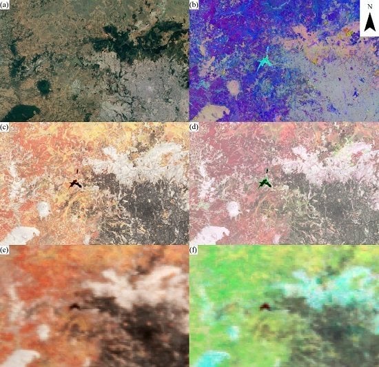
Because SR NDIs outperformed the original TOA and SR images, the Landsat multi-temporal composites were constructed using the SR NDIs instead of the original spectral bands. Examples of the multi-temporal composites are presented in Figure 2 for an area covering parts of Addis Ababa and its vicinity. In Figure 2a, the area in the south-east is highly urbanized, while patches of dense forest exist immediately in the north and with some distance to the west of Addis Ababa. The majority of land in the north and west of Figure 2 are cultivated fields, visualized mainly as light brown in Figure 2a. Gefersa reservoir is located approximately in the center of Figure 2a. Figure 2b shows the Landsat NDVI sinusoidal model fitted independently to time-series data for each pixel. Red green blue (RGB) colors in Figure 2b correspond to the coefficients in Equation (2). As different land-cover classes have different NDVI model amplitudes and phase shifts, the sinusoidal model coefficients can differentiate them. Figure 2c illustrates the Landsat PDF composites with 95%, 75%, 50% of NDI4, i.e., NDVI, as RGB colors. The urban area and Gefersa reservoir appear dark as they have low NDVI value distributions. Forest patches appear very bright as NDVI values are larger for longer periods of time compared to the other classes. Cultivated fields appear as red/yellow as they have high NDVI at some periods and lower NDVI at other periods of the year. Figure 2d shows the Landsat sequential composites with the median of NDI4, i.e., NDVI, from seasons 4,2,1 (see Section 2.3.2) as RGB colors. Similar to Figure 2c vegetated and non-vegetated classes can be differentiated in Figure 2d due to the differences in their ranges of NDVI values. Due to differences in their phenology patterns, forest patches are differentiated from cultivated fields, mainly because forested areas have large NDVI for longer periods of the year. While NDI4, i.e., NDVI, was used for visualization of the Landsat composites in Figure 2c,d, the other NDIs also seemed effective in differentiating the target land-cover classes. The MODIS PDF composite, represented in Figure 2e where RGB colors correspond to the per-pixel 95%, 75%, and 50% of NDVI values, is similar to the Landsat PDF composite in Figure 2c but with lower spatial resolution. The MODIS sequential composite is shown in Figure 2f as the median of NDVI, for June 2016, October 2016, and January 2017 as RGB. Cultivated areas have high NDVI in October but low NDVI in January, therefore, they appear mostly as green/yellow in Figure 2f. Forested areas appear as white/cyan as they have higher NDVI compared to the other classes especially in January.
Overall, the inclusion of any multi-temporal composite, in addition to single-time and textural layers, improved overall classification accuracy (OA). The largest improvement in OA was obtained by the addition of the Landsat sequential composites, which resulted in 3.1% improvement in OA (classification 7 in Table 2), followed by inclusion of the Landsat PDF composites and sinusoidal models (classifications 6 and 5 in Table 2) with 2.7% and 2.1% improvement in OA, respectively. In terms of a comparison between Landsat and MODIS composites, Landsat composites resulted in larger OA improvements than MODIS for both PDF and sequential compositing methods. The advantage of Landsat over MODIS was 1.0% and 1.2% for PDF (classifications 6 and 8 in Table 2) and sequential composites (classifications 7 and 9), respectively. The performances of the two methods of compositing were similar with slight advantages of sequential over PDF compositing; the advantages were 0.4% (classifications 7 and 6 in Table 2) and 0.2% (classifications 9 and 8 in Table 2) for Landsat and MODIS compositing, respectively. In classification 10, where all the Landsat and MODIS composites were used as additional variables to the single-time and textural layers, classification OA improved by 5.1%, which was larger than improvements achieved by each of the multi-temporal composites (classifications 5–9 in Table 2) individually. Generally, Cultivated, Savanna, and Bare Soil classes benefited the most from multi-temporal composites. The largest improvement was obtained for UA of the Bare Soil class that was 16.4%. The Dense Forest, Urban/Built, and Water/Wetland classes did not improve substantially with the addition of multi-temporal composites and in some cases classification accuracy decreased for those classes, especially PA of the Urban/Built class (Table 2). This might be attributed to the fact that spectral signatures of those classes, especially Urban/Built and Water/Wetland, have fewer variations compared to the other classes over different seasons and benefited less from multi-temporal compositing.
Night-time light data from the VIIRS DNB and SRTM elevation dataset were evaluated as ancillary explanatory variables to improve land-cover characterization (classifications 11 and 12 in Table 2). Night-time data improved PA of the Urban/Built class by1.9%; however, UA for this class decreased by 9.6%. This can be partly explained by the blooming effect of night-time data, i.e., the expansion of light beyond urban boundaries, which can lead to an over-estimation of urban areas. Overall, the DNB dataset did not improve classification OA. On the other hand, incorporation of elevation and its derivatives, slope and aspect, improved classification OA by 3.1% (classification 12 in Table 2). This was the classification where all 108 explanatory variables were utilized. Class-specific accuracies also improved by an average of around 2.8%. Classification 13 in Table 2 shows the results of the classification where single-time NDIs were excluded. Exclusion of single-time NDIs decreased classification OA by 2.6%. This suggests that even though multi-temporal information of a sensor, Landsat 8 here, is employed in a classification process, the classification might still benefit from inclusion of single-time image mosaics, if cloud-free images, from a relatively short period, exist for the entire case study.
3.2. Comparison with the Existing Land-Cover Products
To further investigate the performance of the classification outputs, the best classification in terms of OA (classification 12 from Table 2), referred to as LC_2017 hereafter, is compared with the two existing contemporary land-cover products for Ethiopia, which are the GlobeLand30 for 2010 at 30 m resolution and the Copernicus Global Land Operations for 2015 at 100 m resolution. As discussed earlier (Section 2.2), these classifications were recoded and resampled to match with LC_2017 classifications. Note that there are some temporal gaps between the two products and LC_2017 classification. Therefore, some of the differences among these products and their accuracies could be related to actual land changes. Consequently, the comparisons in this section are performed to provide some context to interpret the relative performance of the proposed method rather than selecting a superior methodology. Figure 3 shows the three land-cover map products. The same test dataset used for accuracy assessment of LC_2017 product (Table 2) was used to evaluate the accuracy of the two existing land-cover products (Table 3). Overall, the Copernicus and LC_2017 classifications outperformed the GlobeLand30 product by more than 10% in overall accuracy (Table 3). The difference between OA of LC_2017 and GlobeLand30 was 11.0% and the difference was statistically significant (p-value < 0.001). The difference between OA of LC_2017 and Copernicus products was minor, 0.7% (p-value = 0.46). Moreover, for most classes, the Copernicus and LC_2017 classifications had larger class-specific accuracies than the GlobeLand30 (Table 3). For the Cultivated class, LC_2017 classification had the largest PA (lowest omission error), 79.0% and the Copernicus map had the largest UA (lowest commission error), 75.3%. As Table 4 shows, the cultivated area was 221,303 km2, 264,511 km2, and 298,831 km2 for the GlobeLand30 (2010), Copernicus (2015), and LC_2017, respectively. Given the temporal order of the three products from 2010 to 2017, increasing rates of cultivation activities were observed, which confirms the recent land transactions and increase in intensified agricultural activities. For the Dense Forest class, a high degree of similarity exists between the Copernicus and LC_2017 products where Dense Forest pixels are mainly existing in the southwestern part of the country, whereas in the GlobeLand30 map many Forest pixels also exist in north, north-west, and eastern parts of the country (Figure 3). Moreover, the area of Dense Forest class varies substantially from 64,505 km2 for the Copernicus map to 139,657 km2 for the GlobeLand30 map. Besides classification error, the discrepancies among Dense Forest estimations can be attributed to some extent to the differences in the Dense Forest class definition by the different products. Considerable disagreements exist among the pattern of coverage of the Bare Soil class in GlobeLand30 map (Figure 3A) and the other two products, where many bare areas are classified as Savanna by GlobeLand30. Consequently, the estimated Bare Soil area in GlobeLand30 is less than half of those in the Copernicus and LC_2017 classifications (Table 4). LC_2017 classification had more than 10% larger UA and PA for the Bare Soil class than the existing land-cover products (Table 3). For the Urban/Built class, LC_2017 classification had notably larger PA, 81.1%, than GlobeLand30 and Copernicus maps, 60.0% and 64.3%, respectively. The Urban/Built class UA of the existing maps, however, was larger than LC_2017 map by an average of 6.5%. Finally, with estimated 100% UA, LC_2017 classification outperformed the existing maps, 55% and 78.1% UA for the GlobeLand30 and Copernicus maps, in terms of Water/Wetland class commission error. Water class PA for the Copernicus map was on average 3.7% larger than those of the other two maps (Table 3).
3.3. Final Classification Production
The final classification product of this work is illustrated in Figure 4. The newly developed map provides a contemporary high spatial resolution land-cover characterization for Ethiopia, enabling investigation of the land transactions. To quantify agricultural expansion due to land transactions, a similar classification process will be utilized to produce land-cover maps for earlier dates and change maps will be produced. As evidenced from the three different coverage products already shown (Figure 3), there appears to have been a significant increase in agricultural coverage across Ethiopia, so the specific locations, transaction types and conversion trajectories becomes an important area of future study. The creation of the national classification, with our user-defined classes (Figure 4) is an essential first step, as is the development of full accuracy analyses and tools for comparison with existing products and with available high-resolution imagery. This research thus sets the stage for substantial, and meaningful additional research.
4. Discussion
Land-cover maps are essential variables to study the dynamics of environment. Human activities, such as urbanization, expansion of agricultural activities, and deforestation, as well as natural phenomena such as wildfire, flooding, and desertification frequently lead to changes in land cover. On the other hand, land-cover change itself can direct subsequent changes in the environment and its inhabitants. Therefore, land-cover mapping is integral to understand types of land change, their magnitude and distribution, and the drivers of change. Remote-sensing data provide practical means to map land cover of large areas in more efficient ways, in terms of time and cost, than traditional methods.
The national land-cover product we created shows that 26% of the land surface is in cultivated land use. This is higher than both the GlobeLand30 and Copernicus products (Table 4). GlobeLand30 was created in 2010 and Copernicus is for 2015 and show 221,303 km2 and 264,511 km2 of area under cultivated uses, compared to our estimate of 298,831 km2. Given that our product is for 2017 much of the differences in area may well relate to actual increases in area under cultivated uses, in part related to increased land transactions. In order to account for the differences across product types, future research will focus on this cultivated class and create a land-cover classification using these same methodologies, now they have been defined, developed and tested to compare increasing cultivated area and locations across Ethiopia from early 2000 through current. The remaining land-cover proportions nationally are 8.8% dense forest cover, 56.7% savanna cover, 7.4 % bare soil, 0.4% urban and built and 0.7% water. Comparing our results to theGlobeLand30 and Copernicus products, we show three times the area in urban/built cover, and less area in savanna cover. While some differences vary by each product, these differences are consistent across both products compared to LC_2017. Increases in urban/built are expected over time, and the increase in cultivated area has come at the expense of savanna vegetation and so these differences are explainable. As already noted previously, there will be some confusion in classes with cultivated and savanna, urban/built and bare soil, and dense forest and savanna and so these potential spectral overlaps will be evaluated in more detail in future work focused specifically on the changes in cultivated land due to increased land transactions.
The land transactions and intensified agricultural activities over the last two decades in Ethiopia have caused considerable environmental change, as well as socio-economic impacts on farmers’ livelihoods. To understand land-cover distribution nationally, within which the land transactions are located, it is necessary to characterize land cover at a national level. Time-series of land-cover characterizations are required to quantify the magnitude of land transactions and their spatial distribution. Consequently, to identify an optimum classification process, we examined several land-cover classifications using remote sensing imagery for Ethiopia and assessed their accuracy in this work.
Large-area land-cover image classification is associated with a spectrum of technical challenges such as cloud cover, radiometric inconsistencies within/between images, and big data processing. Consequently, classification accuracy for large-area land-cover products are usually less than those of small area single-scene classifications and in many cases the qualities of the final products might not be sufficient for the intended applications. For example, Yang et al. [109] investigated the accuracy of seven land-cover products over China and reported that overall accuracies ranged from 31.9% to 58.7%. A study of 64 global and regional land-cover products revealed that except in a small number of cases, the reported overall accuracies of most products ranged from 60% to 80% [110]. In addition, spatial variations are likely present in classification accuracies of land-cover products, which might increase as the size of the target area and the number of scenes increases [111,112,113,114,115].
Achieving the target quality could be challenging in large-area mapping projects, as it might require revising classification process/data and investigating multiple classification improvement avenues, which would require considerable effort, time, and budget. These requirements commonly confine analysts’ ability to implement and examine several classification processes to determine which processes and input data are more appropriate for their specific case-study. Therefore, in this research, the classification was replicated using Landsat 8 TOA, SR, and SR NDIs’ variables and the best-performing variable set was identified. In addition, different image compositing methods were investigated to quantify their relative performances.
On review, the NDIs outperformed the original spectral bands. The advantage of the spectral derivatives over the original bands may be attributed to the fact that the derivatives are differences and ratios of bands and are less affected by within and between image radiometric variations. Also, SR images resulted in larger classification OA than TOA images. In addition, multi-temporal composites improved classification accuracies. The advantage of multi-temporal composites is that they are constructed based on time-series of images experiencing broad ranges of sun illumination and atmospheric conditions. These composites can communicate longer-term characteristics of land objects and, therefore, could be more consistent than single-time images that represent only a single snapshot of the case study. Landsat multi-temporal composites resulted in larger OA improvements than MODIS composites. However, because of shorter revisit time, MODIS composites might be more helpful than Landsat composites when short time series of data are being analyzed or when the classification area experiences frequent cloud cover and less probability of clear observations. Sequential composites outperformed PDF composites for both Landsat and MODIS sensors, although the differences were small. Sequential composites could be especially useful with delineating target classes when different target classes have different phenology across a year, such as for Cultivated versus Dense Forest, as in this study (see Figure 2). On the other hand, PDF compositing might be prioritized over sequential compositing for areas with consistent cloud cover where there might not exist enough observations for some months/seasons/periods. In addition, timing of vegetation phenology and agricultural activities could vary over large areas, especially when the target area covers a wide range of latitudes. This can lead to within-class variations of variables of sequential composites. In such cases, PDF composites might provide more consistency than sequential composites, as PDF composites model the overall distributions of spectral values independent from their timing. Moreover, a combination of Landsat and MODIS multi-temporal composites outperformed each of them individually. This means that the two datasets provide complementary information for classification purposes. The efficacy of multi-temporal composites depends on the classification scheme target classes as well. For instance, Urban/Built and Water/Wetland did not largely benefit from those composites in this study as these classes have limited variation over different seasons. Moreover, night-time light data decreased omission error but at the cost of increasing commission error, partly due to a blooming effect. Depending on the application of a target map and effects of those errors on subsequent analyses, an analyst might prioritize one type of error over another. Finally, elevation data and its derivatives as ancillary explanatory variables improved classification accuracy.
5. Conclusions
In this research we examined the effects of several factors on the accuracy of land-cover map production at a national level. The Landsat 8 OLI surface reflectance products are aimed to provide spectral consistency among images captured from different scenes. However, replacing the top of atmosphere images with their corresponding reflectance images resulted in a moderate improvement of 1.1% in classification overall accuracy (OA) in this research. On the other hand, a simple substitution of the original spectral bands with normalized difference spectral indices resulted in an improvement of 1.0% in OA. Therefore, replacement of the original bands with spectral indices might be considered by image analysts, especially for situations (or sensors) where surface reflectance products are not available. The largest improvement (5.1% improvement in the classification OA with respect to the single-time classification) was achieved by the application of the multi-time image composites. Overall, Landsat time-series composites resulted in larger OA improvements than MODIS for both probability density function (PDF) and sequential compositing methods. Among the three approaches for multi-temporal image compositing, the sequential composites slightly outperformed the PDF and sinusoidal composites. The elevation data and its derivatives improved classification accuracy by 1.7%. The night-time light data improve producer’s accuracy of the Urban/Built class with the cost of decreasing its user’s accuracy. Results from this research can aid map producers with decisions related to operational large-area land-cover mapping projects, especially with selecting input explanatory variables and multi-temporal image compositing.
In our future work, we will examine additional methods to improve LC_2017 classification such as incorporation of active sensor data, alternative radiometric normalization methods, object-based image analysis methods, and post-processing techniques. Additional analysis will be conducted on the Cultivated class to separate smallholder fields from industrial fields. To quantify rates and locations of land-cover change in Ethiopia, especially those that are due to recent agricultural land transactions, a similar classification will be conducted for the years 2005–2006 and will be used for post-classification change detection. Developing these methods now allows for multiple applications across multiple dates for more accurate land-cover change analyses.
The land-cover map produced in this research provides up-to-date land information that is reproducible and accurate such that we can use this as a base map for future work, specifically the creation of a 2005–2006 land-cover national product to more fully evaluate the impact of increased land transactions and thus cultivated area, across Ethiopia. Such information is vital to study land transactions, as those changes have been occurring and accelerating over the last 10–15 years. Indeed, a frequent time-series of consistent and well validated accurate land-cover maps is required to investigate land transactions, a highly-paced land change phenomenon of national importance. Creation of such land-cover products, however, is effort/time consuming but essential to develop in-depth understanding of the land transaction practice. Based on the classification process developed in this research, we can now create earlier land-cover classifications for Ethiopia, which will allow for better understanding and quantification/identification of land transactions. In addition, such national land-cover maps can be utilized in global or regional studies of carbon, climate, ecosystem services, deforestation, and so on. This study benefits such studies by developing reproducible techniques for land-use land-cover mapping, enabling understanding of environmental processes, and establishing protocols and methodologies for such construction.
Author Contributions
Conceptualization, R.K. and J.S.; methodology, R.K., J.S., C.M., and T.C.; software, R.K. and C.M.; validation, R.K. and C.M.; formal analysis, R.K.; data curation, C.M.; writing—original draft preparation, R.K., J.S., and C.M.; writing—review and editing, T.C., C.L., A.N.A., D.G.B., and A.A.; supervision, J.S., D.G.B., and A.A.; funding acquisition, J.S., D.G.B., and A.A. All authors have read and agreed to the published version of the manuscript.
Funding
This research was funded from a National Science Foundation grant (award# 1617364); CNH-L: Land Transactions and Investments: Impacts on Agricultural Production, Ecosystem Services, and Food-Energy Security.
Conflicts of Interest
The authors declare no conflict of interest.
References
- Geist, H. Exploring the Entry Points for Political Ecology in the International Research Agenda on Global Environmental Change. Z. Wirtsch. Geogr. 1999, 43, 158–168. [Google Scholar] [CrossRef]
- Lambin, E.F.; Turner, B.L.; Geist, H.J.; Agbola, S.B.; Angelsen, A.; Bruce, J.W.; Coomes, O.T.; Dirzo, R.; Fischer, G.; Folke, C.; et al. The Causes of Land-use and Land-Cover Change: Moving Beyond the Myths. Glob. Environ. Chang. 2001, 11, 261–269. [Google Scholar] [CrossRef]
- Turner, B.L., II; Clark, W.C.; Kates, R.W.; Richards, J.F.; Mathews, J.T.; Meyer, W.B. The Earth as Transformed by Human Action: Global Change and Regional Changes in the Biosphere over the Past 300 Years. In The Earth as Transformed by Human Action: Global Change and Regional Changes in the Biosphere Over the Past 300 Years; Cambridge University Press, with Clark University: Cambridge, UK, 1990. [Google Scholar]
- Kinnaird, M.F.; Sanderson, E.W.; O’Brien, T.G.; Wibisono, H.T.; Woolmer, G. Deforestation Trends in a Tropical Landscape and Implications for Endangered Large Mammals. Conserv. Biol. 2003, 17, 245–257. [Google Scholar] [CrossRef]
- Pimm, S.L.; Russell, G.J.; Gittleman, J.L.; Brooks, T.M. The Future of Biodiversity. Science 1995, 269, 347–350. [Google Scholar] [CrossRef] [PubMed] [Green Version]
- Geist, H.J.; Lambin, E.F. Proximate Causes and Underlying Driving Forces of Tropical Deforestation. Bioscience 2002, 52, 143–150. [Google Scholar] [CrossRef]
- NRC. Our Common Journey: A Transition Toward Sustainability; National Academy Press: Washington, DC, USA, 1999.
- Moran, E.F.; Brondizio, E.S.; Mausel, P.; You, W. Deforestation in Amazonia: Land use Change from Ground and Space Level Perspective. Bioscience 1994, 44, 329–339. [Google Scholar] [CrossRef]
- Hall, R. Land Grabbing in Southern Africa: The Many Faces of the Investor Rush. Rev. Afr. Polit. Econ. 2011, 38, 193–214. [Google Scholar] [CrossRef]
- Borras, S.M., Jr.; Hall, R.; Scoones, I.; White, B.; Wolford, W. Towards a Better Understanding of Global Land Grabbing: An Editorial Introduction. J. Peasant Stud. 2011, 38, 209–216. [Google Scholar] [CrossRef] [Green Version]
- De Schutter, O. How Not to Think of Land-Grabbing: Three Critiques of Large-Scale Investments in Farmland. J. Peasant Stud. 2011, 38, 249–279. [Google Scholar] [CrossRef]
- Deininger, K.; Byerlee, D.; Lindsay, J.; Norton, A.; Selod, H.; Stickler, M. Rising Global Interest in Farmland: Can it Yield Sustainable and Equitable Benefits? Agriculture and Rural Development; World Bank: Washington, DC, USA, 2011. [Google Scholar]
- Robertson, B.; Pinstrup-Andersen, P. Global Land Acquisition: Neo-Colonialism or Development Opportunity? Food Secur. 2010, 2, 271–283. [Google Scholar] [CrossRef]
- Adnan, S. Land Grabs and Primitive Accumulation in Deltaic Bangladesh: Interactions between Neoliberal Globalization, State Interventions, Power Relations and Peasant Resistance. J. Peasant Stud. 2013, 40, 87–128. [Google Scholar] [CrossRef]
- Feldman, S.; Geisler, C. Land Expropriation and Displacement in Bangladesh. J. Peasant Stud. 2012, 39, 971–993. [Google Scholar] [CrossRef]
- White, B.J. Gendered Experiences of Dispossession: Oil Palm Expansion in a Dayak Hibun Community in West Kalimantan. J. Peasant Stud. 2012, 39, 995–1016. [Google Scholar] [CrossRef]
- D’Odorico, P.; Rulli, M.C. The Fourth Food Revolution. Nat. Geosci. 2013, 6, 417–418. [Google Scholar] [CrossRef]
- Davis, K.F.; D’Odorico, P.; Rulli, M.C. Land Grabbing: A Preliminary Quantification of Economic Impacts on Rural Livelihoods. Popul. Environ. 2014, 36, 180–192. [Google Scholar] [CrossRef] [PubMed] [Green Version]
- Cristina Rulli, M.; D’Odorico, P. Food Appropriation through Large Scale Land Acquisitions. Environ. Res. Lett. 2014, 9. [Google Scholar] [CrossRef]
- Gingembre, M. Resistance or Participation? Fighting Against Corporate Land Access Amid Political Uncertainty in Madagascar. J. Peasant Stud. 2015, 42, 561–584. [Google Scholar] [CrossRef]
- Davis, K.F.; Yu, K.; Rulli, M.C.; Pichdara, L.; D’Odorico, P. Accelerated Deforestation Driven by Large-Scale Land Acquisitions in Cambodia. Nat. Geosci. 2015, 8, 772–775. [Google Scholar] [CrossRef] [Green Version]
- Chen, J.; Chen, J.; Liao, A.; Cao, X.; Chen, L.; Chen, X.; He, C.; Han, G.; Peng, S.; Lu, M.; et al. Global Land Cover Mapping at 30 M Resolution: A POK-Based Operational Approach. ISPRS J. Photogramm. Remote Sens. 2014, 103, 7–27. [Google Scholar] [CrossRef] [Green Version]
- Defries, R.S.; Townshend, J.R.G. Global Land Cover Characterization from Satellite Data: From Research to Operational Implementation? Global Ecol. Biogeogr. 1999, 8, 367–379. [Google Scholar] [CrossRef]
- Hansen, M.C.; Loveland, T.R. A Review of Large Area Monitoring of Land Cover Change using Landsat Data. Remote Sens. Environ. 2012, 122, 66–74. [Google Scholar] [CrossRef]
- Xian, G.; Homer, C.; Fry, J. Updating the 2001 National Land Cover Database Land Cover Classification to 2006 by using Landsat Imagery Change Detection Methods. Remote Sens. Environ. 2009, 113, 1133–1147. [Google Scholar] [CrossRef] [Green Version]
- Gorelick, N.; Hancher, M.; Dixon, M.; Ilyushchenko, S.; Thau, D.; Moore, R. Google Earth Engine: Planetary-Scale Geospatial Analysis for Everyone. Remote Sens. Environ. 2017, 202, 18–27. [Google Scholar] [CrossRef]
- Hansen, M.C.; Potapov, P.V.; Moore, R.; Hancher, M.; Turubanova, S.A.; Tyukavina, A.; Thau, D.; Stehman, S.V.; Goetz, S.J.; Loveland, T.R.; et al. High-Resolution Global Maps of 21st-Century Forest Cover Change. Science 2013, 342, 850–853. [Google Scholar] [CrossRef] [Green Version]
- Dong, J.; Xiao, X.; Menarguez, M.A.; Zhang, G.; Qin, Y.; Thau, D.; Biradar, C.; Moore, B., III. Mapping Paddy Rice Planting Area in Northeastern Asia with Landsat 8 Images, Phenology-Based Algorithm and Google Earth Engine. Remote Sens. Environ. 2016, 185, 142–154. [Google Scholar] [CrossRef] [Green Version]
- Lobell, D.B.; Thau, D.; Seifert, C.; Engle, E.; Little, B. A Scalable Satellite-Based Crop Yield Mapper. Remote Sens. Environ. 2015, 164, 324–333. [Google Scholar] [CrossRef]
- Xiong, J.; Thenkabail, P.S.; Gumma, M.K.; Teluguntla, P.; Poehnelt, J.; Congalton, R.G.; Yadav, K.; Thau, D. Automated Cropland Mapping of Continental Africa using Google Earth Engine Cloud Computing. ISPRS J. Photogramm. Remote Sens. 2017, 126, 225–244. [Google Scholar] [CrossRef] [Green Version]
- Kennedy, R.E.; Yang, Z.; Gorelick, N.; Braaten, J.; Cavalcante, L.; Cohen, W.B.; Healey, S. Implementation of the LandTrendr Algorithm on Google Earth Engine. Remote Sens. 2018, 10, 691. [Google Scholar] [CrossRef] [Green Version]
- Huntington, J.; McGwire, K.; Morton, C.; Snyder, K.; Peterson, S.; Erickson, T.; Niswonger, R.; Carroll, R.; Smith, G.; Allen, R. Assessing the Role of Climate and Resource Management on Groundwater Dependent Ecosystem Changes in Arid Environments with the Landsat Archive. Remote Sens. Environ. 2016, 185, 186–197. [Google Scholar] [CrossRef] [Green Version]
- Sazib, N.; Mladenova, I.; Bolten, J. Leveraging the Google Earth Engine for Drought Assessment using Global Soil Moisture Data. Remote Sens. 2018, 10, 1265. [Google Scholar] [CrossRef] [Green Version]
- Goldblatt, R.; Stuhlmacher, M.F.; Tellman, B.; Clinton, N.; Hanson, G.; Georgescu, M.; Wang, C.; Serrano-Candela, F.; Khandelwal, A.K.; Cheng, W.-H.; et al. Using Landsat and Nighttime Lights for Supervised Pixel-Based Image Classification of Urban Land Cover. Remote Sens. Environ. 2018, 205, 253–275. [Google Scholar] [CrossRef]
- Liu, X.; Hu, G.; Chen, Y.; Li, X.; Xu, X.; Li, S.; Pei, F.; Wang, S. High-Resolution Multi-Temporal Mapping of Global Urban Land using Landsat Images Based on the Google Earth Engine Platform. Remote Sens. Environ. 2018, 209, 227–239. [Google Scholar] [CrossRef]
- Patela, N.N.; Angiuli, E.; Gamba, P.; Gaughan, A.; Lisini, G.; Stevens, F.R.; Tatem, A.J.; Trianni, G. Multitemporal Settlement and Population Mapping from Landsatusing Google Earth Engine. Int. J. Appl. Earth Obs. Geoinf. 2015, 35, 199–208. [Google Scholar] [CrossRef] [Green Version]
- Trianni, G.; Lisini, G.; Angiuli, E.; Moreno, E.A.; Dondi, P.; Gaggia, A.; Gamba, P. Scaling Up to National/Regional Urban Extent Mapping using Landsat Data. IEEE J. Sel. Top. Appl. Earth Obs. Remote Sens. 2015, 8, 3710–3719. [Google Scholar] [CrossRef]
- Huang, H.; Chen, Y.; Clinton, N.; Wang, J.; Wang, X.; Liu, C.; Gong, P.; Yang, J.; Bai, Y.; Zheng, Y.; et al. Mapping Major Land Cover Dynamics in Beijing using all Landsat Images in Google Earth Engine. Remote Sens. Environ. 2017, 202, 166–176. [Google Scholar] [CrossRef]
- Simonetti, D.; Simonetti, E.; Szantoi, Z.; Lupi, A.; Eva, H.D. First Results from the Phenology-Based Synthesis Classifier using Landsat 8 Imagery. IEEE Geosci. Remote Sens. Lett. 2015, 12, 1496–1500. [Google Scholar] [CrossRef]
- Wang, J.; Xiao, X.; Qin, Y.; Doughty, R.B.; Dong, J.; Zou, Z. Characterizing the Encroachment of Juniper Forests into Sub-Humid and Semi-Arid Prairies from 1984 to 2010 using PALSAR and Landsat Data. Remote Sens. Environ. 2018, 205, 166–179. [Google Scholar] [CrossRef]
- Shrestha, D.P.; Saepuloh, A.; van der Meer, F. Land Cover Classification in the Tropics, Solving the Problem of Cloud Covered Areas using Topographic Parameters. Int. J. Appl. Earth Obs. Geoinf. 2019, 77, 84–93. [Google Scholar] [CrossRef]
- Canty, M.J.; Nielsen, A.A.; Schmidt, M. Automatic Radiometric Normalization of Multitemporal Satellite Imagery. Remote Sens. Environ. 2004, 91, 441–451. [Google Scholar] [CrossRef] [Green Version]
- Yang, X.; Lo, C.P. Relative Radiometric Normalization Performance for Change Detection from Multi-Date Satellite Images. Photogramm. Eng. Remote Sens. 2000, 66, 967–980. [Google Scholar]
- Zhou, H.; Liu, S.; He, J.; Wen, Q.; Song, L.; Ma, Y. A New Model for the Automatic Relative Radiometric Normalization of Multiple Images with Pseudo-Invariant Features. Int. J. Remote Sens. 2016, 37, 4554–4573. [Google Scholar] [CrossRef]
- Harper, G.J.; Steininger, M.K.; Tucker, C.J.; Juhn, D.; Hawkins, F. Fifty Years of Deforestation and Forest Fragmentation in Madagascar. Environ. Conserv. 2007, 34, 325–333. [Google Scholar] [CrossRef]
- Killeen, T.J.; Calderon, V.; Soria, L.; Quezada, B.; Steininger, M.K.; Harper, G.; Solórzano, L.A.; Tucker, C.J. Thirty Years of Land-Cover Change in Bolivia. Ambio 2007, 36, 600–606. [Google Scholar] [CrossRef] [Green Version]
- Leimgruber, P.; Kelly, D.S.; Steininger, M.K.; Brunner, J.; Müller, T.; Songer, M. Forest Cover Change Patterns in Myanmar (Burma) 1990–2000. Environ. Conserv. 2005, 32, 356–364. [Google Scholar] [CrossRef] [Green Version]
- Xian, G.; Homer, C. Updating the 2001 National Land Cover Database Impervious Surface Products to 2006 using Landsat Imagery Change Detection Methods. Remote Sens. Environ. 2010, 114, 1676–1686. [Google Scholar] [CrossRef]
- Arévalo, P.; Olofsson, P.; Woodcock, C.E. Continuous Monitoring of Land Change Activities and Post-Disturbance Dynamics from Landsat Time Series: A Test Methodology for REDD+ Reporting. Remote Sens. Environ. 2019, 238, 111051. [Google Scholar] [CrossRef]
- Khatami, R.; Mountrakis, G.; Stehman, S.V. A Meta-Analysis of Remote Sensing Research on Supervised Pixel-Based Land-Cover Image Classification Processes: General Guidelines for Practitioners and Future Research. Remote Sens. Environ. 2016, 177, 89–100. [Google Scholar] [CrossRef] [Green Version]
- Novo-Fernández, A.; Franks, S.; Wehenkel, C.; López-Serrano, P.M.; Molinier, M.; López-Sánchez, C.A. Landsat Time Series Analysis for Temperate Forest Cover Change Detection in the Sierra Madre Occidental, Durango, Mexico. Int. J. Appl. Earth Obs. Geoinf. 2018, 73, 230–244. [Google Scholar] [CrossRef]
- Tang, X.; Bullock, E.L.; Olofsson, P.; Estel, S.; Woodcock, C.E. Near Real-Time Monitoring of Tropical Forest Disturbance: New Algorithms and Assessment Framework. Remote Sens. Environ. 2019, 224, 202–218. [Google Scholar] [CrossRef]
- Zhu, Z. Change Detection using Landsat Time Series: A Review of Frequencies, Preprocessing, Algorithms, and Applications. ISPRS J. Photogramm. Remote Sens. 2017, 130, 370–384. [Google Scholar] [CrossRef]
- Baumann, M.; Ozdogan, M.; Richardson, A.D.; Radeloff, V.C. Phenology from Landsat when Data is Scarce: Using MODIS and Dynamic Time-Warping to Combine Multi-Year Landsat Imagery to Derive Annual Phenology Curves. Int. J. Appl. Earth Obs. Geoinf. 2017, 54, 72–83. [Google Scholar] [CrossRef]
- Goldblatt, R.; You, W.; Hanson, G.; Khandelwal, A.K. Detecting the Boundaries of Urban Areas in India: A Dataset for Pixel-Based Image Classification in Google Earth Engine. Remote Sens. 2016, 8, 634. [Google Scholar] [CrossRef] [Green Version]
- Gómez-Chova, L.; Amorós-López, J.; Mateo-García, G.; Muñoz-Marí, J.; Camps-Valls, G. Cloud Masking and Removal in Remote Sensing Image Time Series. J. Appl. Remote Sens. 2017, 11. [Google Scholar] [CrossRef]
- Shelestov, A.; Lavreniuk, M.; Kussul, N.; Novikov, A.; Skakun, S. Exploring Google Earth Engine Platform for Big Data Processing: Classification of Multi-Temporal Satellite Imagery for Crop Mapping. Front. Earth Sci. 2017, 5, 17. [Google Scholar] [CrossRef] [Green Version]
- Testa, S.; Soudani, K.; Boschetti, L.; Borgogno Mondino, E. MODIS-Derived EVI, NDVI and WDRVI Time Series to Estimate Phenological Metrics in French Deciduous Forests. Int. J. Appl. Earth Obs. Geoinf. 2018, 64, 132–144. [Google Scholar] [CrossRef]
- Azzari, G.; Lobell, D.B. Landsat-Based Classification in the Cloud: An Opportunity for a Paradigm Shift in Land Cover Monitoring. Remote Sens. Environ. 2017, 202, 64–74. [Google Scholar] [CrossRef]
- Broich, M.; Hansen, M.C.; Potapov, P.; Adusei, B.; Lindquist, E.; Stehman, S.V. Time-Series Analysis of Multi-Resolution Optical Imagery for Quantifying Forest Cover Loss in Sumatra and Kalimantan, Indonesia. Int. J. Appl. Earth Obs. Geoinf. 2011, 13, 277–291. [Google Scholar] [CrossRef]
- Hansen, M.C.; Egorov, A.; Potapov, P.V.; Stehman, S.V.; Tyukavina, A.; Turubanova, S.A.; Roy, D.P.; Goetz, S.J.; Loveland, T.R.; Ju, J.; et al. Monitoring Conterminous United States (CONUS) Land Cover Change with Web-Enabled Landsat Data (WELD). Remote Sens. Environ. 2014, 140, 466–484. [Google Scholar] [CrossRef] [Green Version]
- Yan, L.; Roy, D.P. Automated Crop Field Extraction from Multi-Temporal Web Enabled Landsat Data. Remote Sens. Environ. 2014, 144, 42–64. [Google Scholar] [CrossRef] [Green Version]
- Zald, H.S.J.; Wulder, M.A.; White, J.C.; Hilker, T.; Hermosilla, T.; Hobart, G.W.; Coops, N.C. Integrating Landsat Pixel Composites and Change Metrics with Lidar Plots to Predictively Map Forest Structure and Aboveground Biomass in Saskatchewan, Canada. Remote Sens. Environ. 2016, 176, 188–201. [Google Scholar] [CrossRef] [Green Version]
- The World Bank. Agribusiness Indicators: Ethiopia; (No. 68237-ET); The World Bank: Washington, DC, USA, 2012; Available online: http://http://documents.worldbank.org/curated/en/631391468008109813/pdf/682370ESW0P1260ators0Ethiopia0final.pdf (accessed on 3 February 2020).
- Teklemariam, D.; Azadi, H.; Nyssen, J.; Haile, M.; Witlox, F. How Sustainable is Transnational Farmland Acquisition in Ethiopia? Lessons Learned from the Benishangul-Gumuz Region. Sustainability 2016, 8, 213. [Google Scholar] [CrossRef] [Green Version]
- The World Factbook 2013–2014; Central Intelligence Agency: Washington, DC, USA, 2013.
- Central Statistical Agency. Agricultural Sample Survey 2015/2016 (No. 1); Ethiopia Central Statistical Agency: Addis Ababa, Ethiopia, 2016.
- Taffessem, A.; Dorosh, P.; Asrat, S. Crop Production in Ethiopia: Regional Patterns and Trends; International Food Policy Research Institute: Washington, DC, USA, 2012. [Google Scholar]
- Horne, F. Understanding Land Investment Deals in Africa; Country Report; Oakland Institute: Oakland, CA, USA, 2011; Available online: https://www.oaklandinstitute.org/sites/oaklandinstitute.org/files/OI_Ethiopa_Land_Investment_report.pdf (accessed on 3 February 2020).
- Hurni, H. Agroecological Belts of Ethiopia. Explanatory Notes on Three Maps at a Scale of 1:1,000 000. Soil Conservation Research Programme (SCRP) and Centre for Development and Environment (CDE). University of Bern, Addis Ababa and Bern. 1998. Available online: https://edepot.wur.nl/484855 (accessed on 3 February 2020).
- Fazzini, M.; Bisci, C.; Billi, P. The Climate of Ethiopia. In Landscapes and Landforms of Ethiopia; World Geomorphological Landscapes; Billi, P., Ed.; Springer: Dordrecht, The Netherlands, 2015. [Google Scholar]
- Alemayehu, A.; Bewket, W. Local Climate Variability and Crop Production in the Central Highlands of Ethiopia. Environ. Dev. 2016, 19, 36–48. [Google Scholar] [CrossRef]
- Biazin, B.; Sterk, G. Drought Vulnerability Drives Land-use and Land Cover Changes in the Rift Valley Dry Lands of Ethiopia. Agric. Ecosyst. Environ. 2013, 164, 100–113. [Google Scholar] [CrossRef]
- Gebru, T. Deforestation in Ethiopia: Causes, Impacts, and Remedy. Int. J. Eng. Dev. Res. 2016, 4, 204. [Google Scholar]
- Minta, M.; Kibret, K.; Thorne, P.; Nigussie, T.; Nigatu, L. Land use and Land Cover Dynamics in Dendi-Jeldu Hilly-Mountainous Areas in the Central Ethiopian Highlands. Geoderma 2018, 314, 27–36. [Google Scholar] [CrossRef]
- Ali, D.A.; Deininger, K.; Harris, A. Using National Statistics to Increase Transparency of Large Land Acquisition: Evidence from Ethiopia. World Dev. 2017, 93, 62–74. [Google Scholar] [CrossRef] [Green Version]
- Tolessa, T.; Senbeta, F.; Kidane, M. The Impact of Land use/Land Cover Change on Ecosystem Services in the Central Highlands of Ethiopia. Ecosyst. Serv. 2017, 23, 47–54. [Google Scholar] [CrossRef]
- Loveland, T.R.; Irons, J.R. Landsat 8: The Plans, the Reality, and the Legacy. Remote Sens. Environ. 2016, 185, 1–6. [Google Scholar] [CrossRef] [Green Version]
- Roy, D.P.; Ju, J.; Mbow, C.; Frost, P.; Loveland, T. Accessing Free Landsat Data Via the Internet: Africa’s Challenge. Remote Sens. Lett. 2010, 1, 111–117. [Google Scholar] [CrossRef]
- Roy, D.P.; Wulder, M.A.; Loveland, T.R.; Woodcock, C.E.; Allen, R.G.; Anderson, M.C.; Helder, D.; Irons, J.R.; Johnson, D.M.; Kennedy, R.; et al. Landsat-8: Science and Product Vision for Terrestrial Global Change Research. Remote Sens. Environ. 2014, 145, 154–172. [Google Scholar] [CrossRef] [Green Version]
- Wulder, M.A.; White, J.C.; Loveland, T.R.; Woodcock, C.E.; Belward, A.S.; Cohen, W.B.; Fosnight, E.A.; Shaw, J.; Masek, J.G.; Roy, D.P. The Global Landsat Archive: Status, Consolidation, and Direction. Remote Sens. Environ. 2016, 185, 271–283. [Google Scholar] [CrossRef] [Green Version]
- Gómez, C.; White, J.C.; Wulder, M.A. Optical Remotely Sensed Time Series Data for Land Cover Classification: A Review. ISPRS J. Photogramm. Remote Sens. 2016, 116, 55–72. [Google Scholar] [CrossRef] [Green Version]
- Woodcock, C.E.; Allen, R.; Anderson, M.; Belward, A.; Bindschadler, R.; Cohen, W.; Gao, F.; Goward, S.N.; Helder, D.; Helmer, E.; et al. Free Access to Landsat Imagery. Science 2008, 320, 1011. [Google Scholar] [CrossRef] [PubMed]
- Wulder, M.A.; Masek, J.G.; Cohen, W.B.; Loveland, T.R.; Woodcock, C.E. Opening the Archive: How Free Data has Enabled the Science and Monitoring Promise of Landsat. Remote Sens. Environ. 2012, 122, 2–10. [Google Scholar] [CrossRef]
- Zhu, Z.; Wulder, M.A.; Roy, D.P.; Woodcock, C.E.; Hansen, M.C.; Radeloff, V.C.; Healey, S.P.; Schaaf, C.; Hostert, P.; Strobl, P.; et al. Benefits of the Free and Open Landsat Data Policy. Remote Sens. Environ. 2019, 224, 382–385. [Google Scholar] [CrossRef]
- Vermote, E.; Justice, C.; Claverie, M.; Franch, B. Preliminary Analysis of the Performance of the Landsat 8/OLI Land Surface Reflectance Product. Remote Sens. Environ. 2016, 185, 46–56. [Google Scholar] [CrossRef] [PubMed]
- Masek, J.G.; Vermote, E.F.; Saleous, N.E.; Wolfe, R.; Hall, F.G.; Huemmrich, K.F.; Gao, F.; Kutler, J.; Lim, T.-K. A Landsat Surface Reflectance Dataset for North America, 1990–2000. IEEE Geosci. Remote Sens. Lett. 2006, 3, 68–72. [Google Scholar] [CrossRef]
- Zhu, Z.; Woodcock, C.E. Object-Based Cloud and Cloud Shadow Detection in Landsat Imagery. Remote Sens. Environ. 2012, 118, 83–94. [Google Scholar] [CrossRef]
- Zhu, Z.; Wang, S.; Woodcock, C.E. Improvement and Expansion of the Fmask Algorithm: Cloud, Cloud Shadow, and Snow Detection for Landsats 4-7, 8, and Sentinel 2 Images. Remote Sens. Environ. 2015, 159, 269–277. [Google Scholar] [CrossRef]
- Wang, L.; Shi, C.; Diao, C.; Ji, W.; Yin, D. A Survey of Methods Incorporating Spatial Information in Image Classification and Spectral Unmixing. Int. J. Remote Sens. 2016, 37, 3870–3910. [Google Scholar] [CrossRef]
- Gong, P.; Wang, J.; Yu, L.; Zhao, Y.; Zhao, Y.; Liang, L.; Niu, Z.; Huang, X.; Fu, H.; Liu, S.; et al. Finer Resolution Observation and Monitoring of Global Land Cover: First Mapping Results with Landsat TM and ETM+ Data. Int. J. Remote Sens. 2013, 34, 2607–2654. [Google Scholar] [CrossRef] [Green Version]
- Khatami, R.; Mountrakis, G. The Interacting Effects of Image Acquisition Date, Number of Images, Classifier, and Number of Training Samples on Accuracy of Binary Classification of Impervious Cover. Remote Sens. Lett. 2018, 9, 189–198. [Google Scholar] [CrossRef]
- Schultz, M.; Clevers, J.G.P.W.; Carter, S.; Verbesselt, J.; Avitabile, V.; Quang, H.V.; Herold, M. Performance of Vegetation Indices from Landsat Time Series in Deforestation Monitoring. Int. J. Appl. Earth Obs. Geoinf. 2016, 52, 318–327. [Google Scholar] [CrossRef]
- Schwieder, M.; Leitão, P.J.; da Cunha Bustamante, M.M.; Ferreira, L.G.; Rabe, A.; Hostert, P. Mapping Brazilian Savanna Vegetation Gradients with Landsat Time Series. Int. J. Appl. Earth Obs. Geoinf. 2016, 52, 361–370. [Google Scholar] [CrossRef]
- Griffiths, P.; Van Der Linden, S.; Kuemmerle, T.; Hostert, P. Erratum: A Pixel-Based Landsat Compositing Algorithm for Large Area Land Cover Mapping (IEEE Journal of Selected Topics in Applied Earth Observations and Remote Sensing). IEEE J. Sel. Top. Appl. Earth Obs. Remote Sens. 2013, 6, 2088–2101. [Google Scholar] [CrossRef]
- Peterson, B.; Nelson, K.J. Mapping Forest Height in Alaska using GLAS, Landsat Composites, and Airborne LiDAR. Remote Sens. 2014, 6, 12409–12426. [Google Scholar] [CrossRef] [Green Version]
- Potapov, P.; Turubanova, S.; Hansen, M.C. Regional-Scale Boreal Forest Cover and Change Mapping using Landsat Data Composites for European Russia. Remote Sens. Environ. 2011, 115, 548–561. [Google Scholar] [CrossRef]
- Sexton, J.O.; Urban, D.L.; Donohue, M.J.; Song, C. Long-Term Land Cover Dynamics by Multi-Temporal Classification Across the Landsat-5 Record. Remote Sens. Environ. 2013, 128, 246–258. [Google Scholar] [CrossRef]
- Sexton, J.O.; Song, X.-P.; Huang, C.; Channan, S.; Baker, M.E.; Townshend, J.R. Urban Growth of the Washington, D.C.-Baltimore, MD Metropolitan Region from 1984 to 2010 by Annual, Landsat-Based Estimates of Impervious Cover. Remote Sens. Environ. 2013, 129, 42–53. [Google Scholar] [CrossRef]
- Workie, T.G.; Debella, H.J. Climate Change and its Effects on Vegetation Phenology Across Ecoregions of Ethiopia. Glob. Ecol. Conserv. 2018, 13, e00366. [Google Scholar] [CrossRef]
- Shumway, R.H.; Stoffe, D.S. Time Series Analysis and its Applications with R Examples, 4th ed.; Springer International Publishing: Cham, Switzerland, 2017; p. 562. [Google Scholar]
- Zhu, Z.; Woodcock, C.E. Continuous Change Detection and Classification of Land Cover using all Available Landsat Data. Remote Sens. Environ. 2014, 144, 152–171. [Google Scholar] [CrossRef] [Green Version]
- Reuter, H.I.; Nelson, A.; Jarvis, A. An Evaluation of Void-Filling Interpolation Methods for SRTM Data. Int. J. Geogr. Inf. Sci. 2007, 21, 983–1008. [Google Scholar] [CrossRef]
- Cai, J.; Huang, B.; Song, Y. Using Multi-Source Geospatial Big Data to Identify the Structure of Polycentric Cities. Remote Sens. Environ. 2017, 202, 210–221. [Google Scholar] [CrossRef]
- Schneider, A.; Friedl, M.A.; McIver, D.K.; Woodcock, C.E. Mapping Urban Areas by Fusing Multiple Sources of Coarse Resolution Remotely Sensed Data. Photogramm. Eng. Remote Sens. 2003, 69, 1377–1386. [Google Scholar] [CrossRef]
- Breiman, L. Random Forests. Mach. Learn. 2001, 45, 5–32. [Google Scholar] [CrossRef] [Green Version]
- Melville, B.; Lucieer, A.; Aryal, J. Object-Based Random Forest Classification of Landsat ETM+ and WorldView-2 Satellite Imagery for Mapping Lowland Native Grassland Communities in Tasmania, Australia. Int. J. Appl. Earth Obs. Geoinf. 2018, 66, 46–55. [Google Scholar] [CrossRef]
- Pelletier, C.; Valero, S.; Inglada, J.; Champion, N.; Dedieu, G. Assessing the Robustness of Random Forests to Map Land Cover with High Resolution Satellite Image Time Series Over Large Areas. Remote Sens. Environ. 2016, 187, 156–168. [Google Scholar] [CrossRef]
- Yang, Y.; Xiao, P.; Feng, X.; Li, H. Accuracy Assessment of Seven Global Land Cover Datasets over China. ISPRS J. Photogramm. Remote Sens. 2017, 125, 156–173. [Google Scholar] [CrossRef]
- Grekousis, G.; Mountrakis, G.; Kavouras, M. An Overview of 21 Global and 43 Regional Land-Cover Mapping Products. Int. J. Remote Sens. 2015, 36, 5309–5335. [Google Scholar] [CrossRef]
- Khatami, R.; Mountrakis, G.; Stehman, S.V. Mapping Per-Pixel Predicted Accuracy of Classified Remote Sensing Images. Remote Sens. Environ. 2017, 191, 156–167. [Google Scholar] [CrossRef] [Green Version]
- Khatami, R.; Mountrakis, G.; Stehman, S.V. Predicting Individual Pixel Error in Remote Sensing Soft Classification. Remote Sens. Environ. 2017, 199, 401–414. [Google Scholar] [CrossRef]
- Tsutsumida, N.; Rodríguez-Veiga, P.; Harris, P.; Balzter, H.; Comber, A. Investigating Spatial Error Structures in Continuous Raster Data. Int. J. Appl. Earth Obs. Geoinf. 2019, 74, 259–268. [Google Scholar] [CrossRef]
- Wickham, J.; Stehman, S.V.; Homer, C.G. Spatial Patterns of the United States National Land Cover Dataset (NLCD) Land-Cover Change Thematic Accuracy (2001–2011). Int. J. Remote Sens. 2018, 39, 1729–1743. [Google Scholar] [CrossRef] [PubMed] [Green Version]
- Zhang, J.; Zhang, W.; Mei, Y.; Yang, W. Geostatistical Characterization of Local Accuracies in Remotely Sensed Land Cover Change Categorization with Complexly Configured Reference Samples. Remote Sens. Environ. 2019, 223, 63–81. [Google Scholar] [CrossRef]
Figure 1.
Examples of the target land-cover classes showing the ranges of class distribution, ordered by land-cover proportion cover of a pixel, from maximum cover to minimum cover to still be assigned to the class, from left to right. Red squares show footprints of Landsat pixels.
Figure 1.
Examples of the target land-cover classes showing the ranges of class distribution, ordered by land-cover proportion cover of a pixel, from maximum cover to minimum cover to still be assigned to the class, from left to right. Red squares show footprints of Landsat pixels.

Figure 2.
Visualization of multi-temporal image composites for Addis Ababa for: (a) high-resolution imagery from Google Earth Engine (GEE); (b) Landsat Normalized Difference Vegetation Index (NDVI) sinusoidal model coefficients, Red green blue (RGB): (see Equation (2));(c) Landsat PDF composite, RGB: 95%, 75%, 50% of NDI4, i.e., NDVI; (d) Landsat sequential composite, RGB: median NDI4, i.e., NDVI, from periods 4,2,1 (see Section 2.3.2); (e) MODIS PDF composite, RGB: 95%, 75%, 50% of NDVI; and (f) MODIS sequential composite, RGB: median NDVI for June 2016, October 2016, and January 2017.

Figure 3.
Comparison of the three different land-cover products: (A) GlobeLand30 for 2010 at 30 m resolution (the straight lines are due to missing data), (B) Copernicus 2015 Land-Cover Product at 100 m resolution, and (C) LC_2017 product for 2017 at 30 m resolution.
Figure 3.
Comparison of the three different land-cover products: (A) GlobeLand30 for 2010 at 30 m resolution (the straight lines are due to missing data), (B) Copernicus 2015 Land-Cover Product at 100 m resolution, and (C) LC_2017 product for 2017 at 30 m resolution.

Figure 4.
Land-cover map of Ethiopia for 2017 at 30 m spatial resolution.


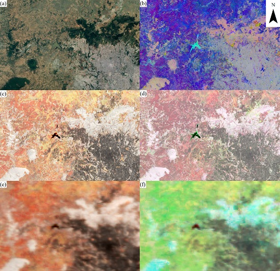
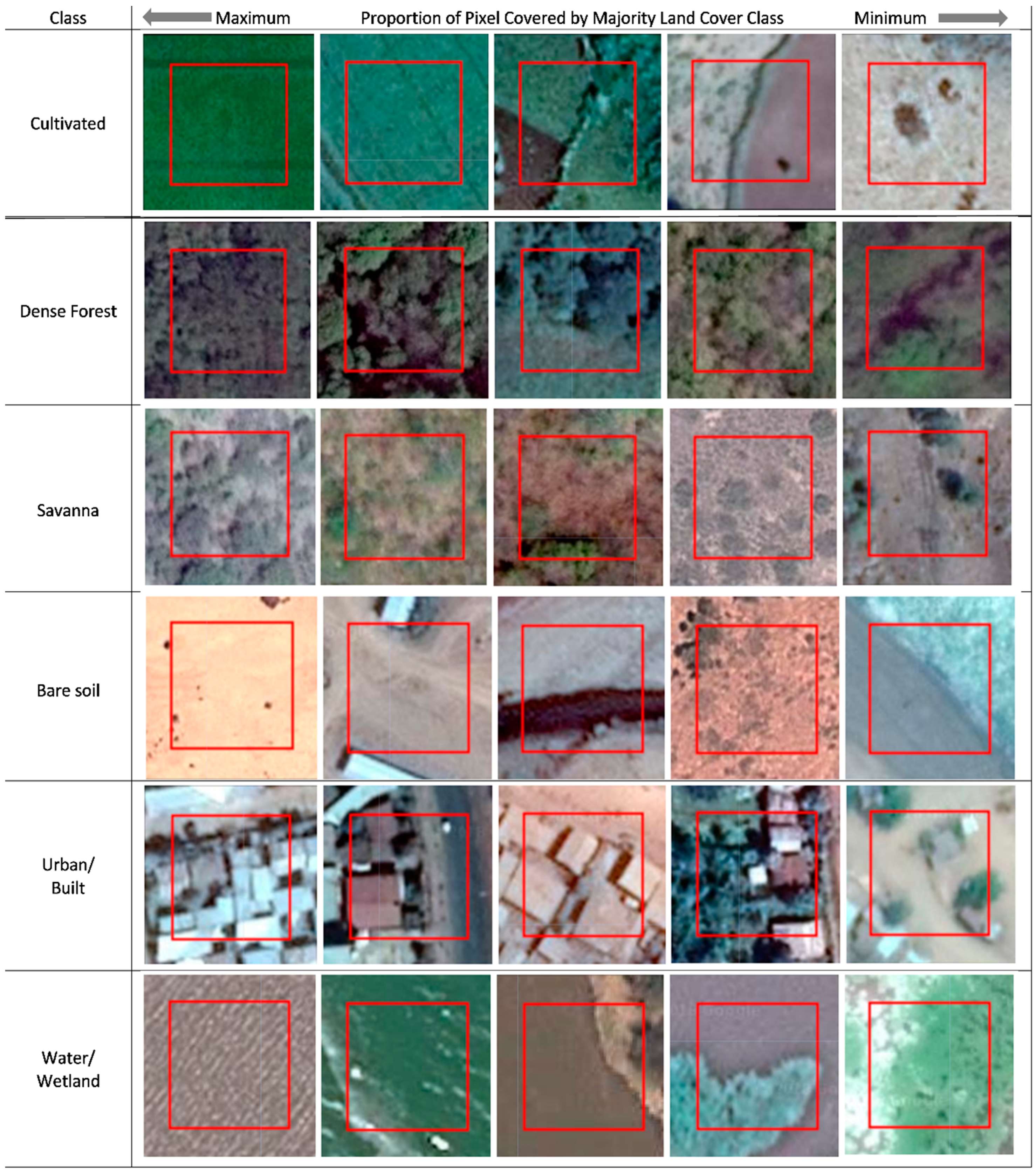
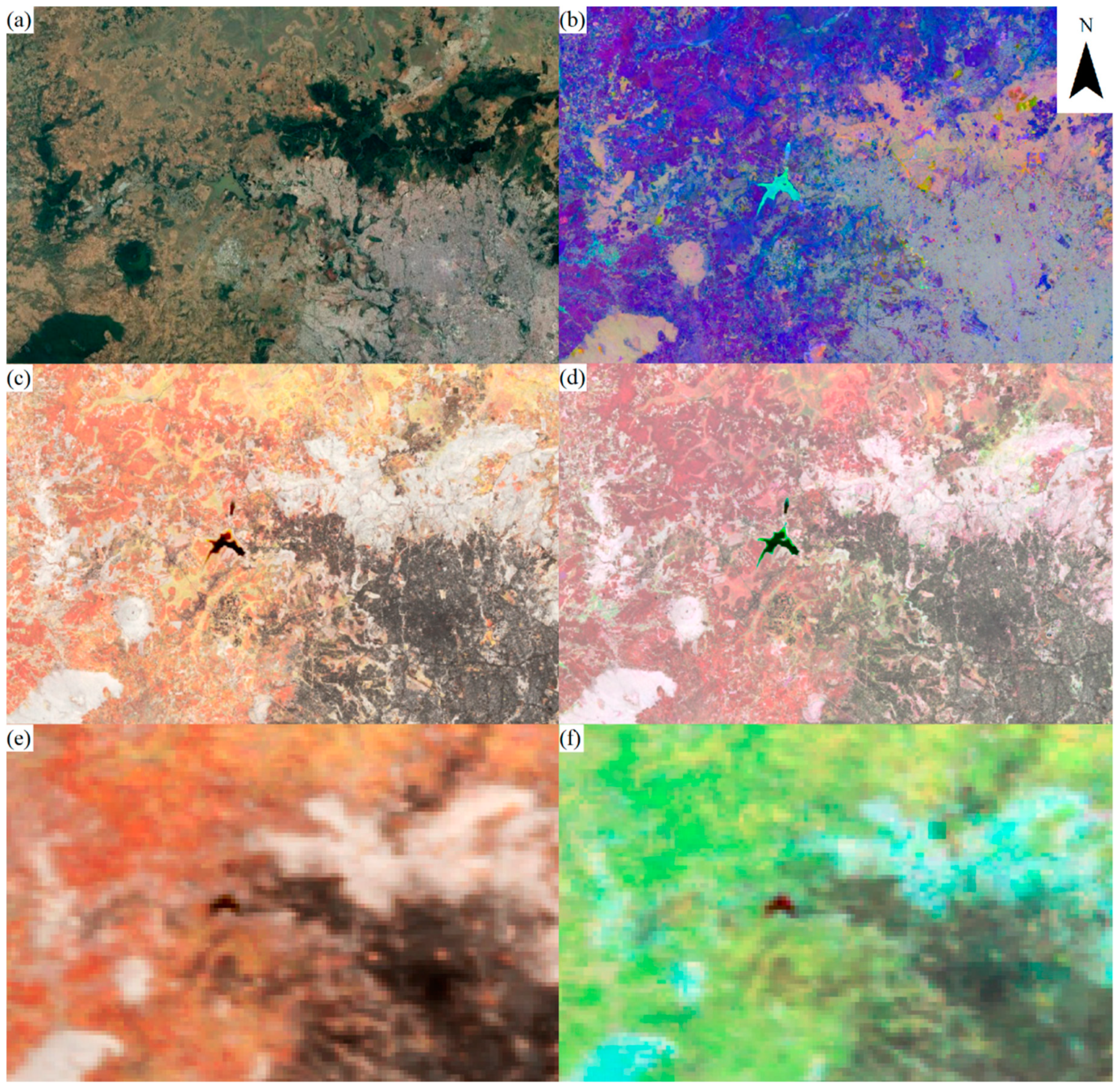
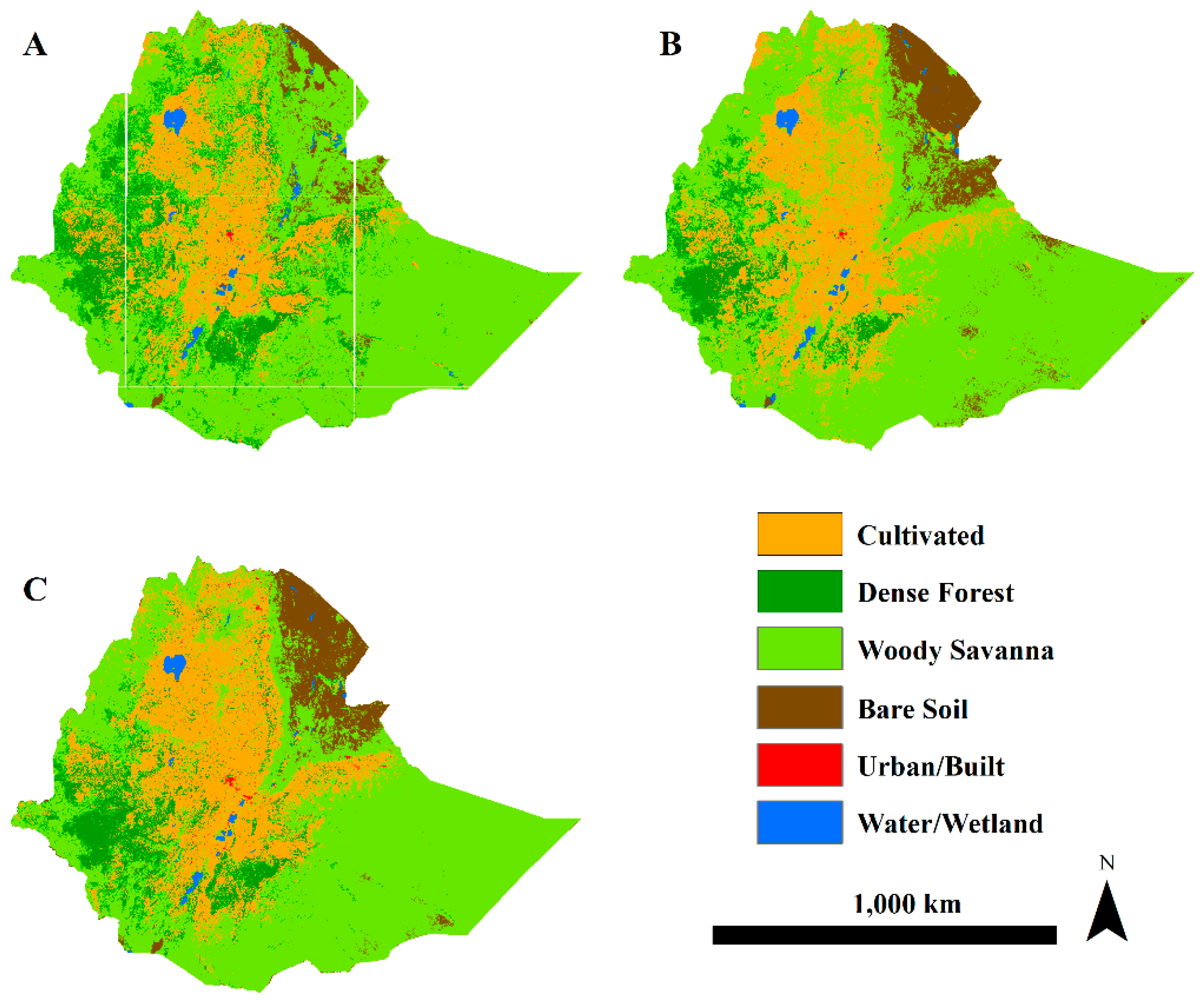
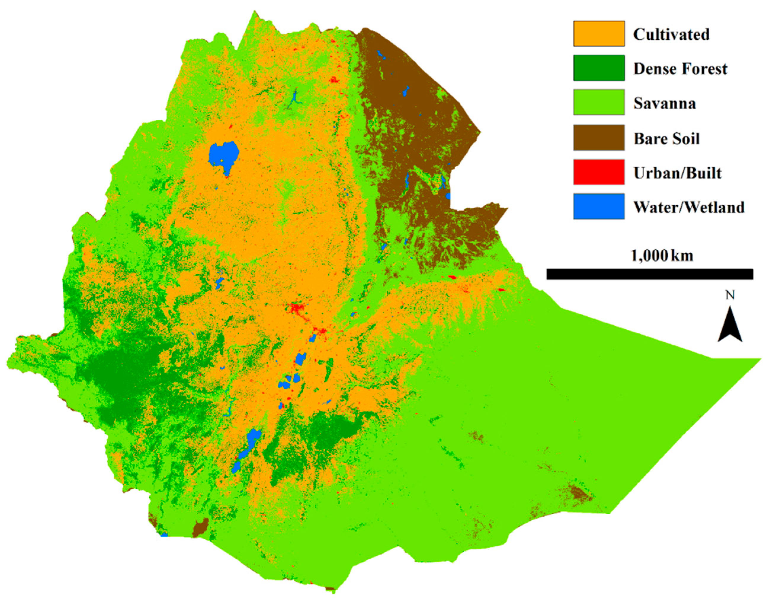
Table 1.
Land-cover classification scheme and corresponding classes in Copernicus and GlobeLand30 map products.
Table 1.
Land-cover classification scheme and corresponding classes in Copernicus and GlobeLand30 map products.
| Land-Cover Class | Class Definition Used in this Work | Corresponding Class in Copernicus | Corresponding Class in GlobLand30 |
|---|---|---|---|
| Dense Forest | Vegetation dominated by tree cover of 70% or greater. | Forest, closed forest (deciduous, evergreen) | Forest |
| Savanna | Grasses, shrubs, herbaceous plants, and tree cover less than 70%. | Shrubs, herbaceous vegetation | Shrubland, grassland |
| Cultivated | Land used for agriculture, small-holder and intensive cultivation, including plantations. | Cultivated and managed vegetation/agriculture | Cultivated land |
| Bare Soil | Bare soil and rock with <5% vegetation cover. | Bare/sparse vegetation | Bareland |
| Urban/Built | Land predominantly covered by man-made structures; roads, buildings. | Urban/built up | Artificial surfaces |
| Water/Wetland | Permanent water bodies (rivers, lakes) or wetlands. | Temporary water bodies, Permanent water bodies | Wetland, water bodies |
Table 2.
Overall and class-specific accuracies (%) of classifications based on different combinations of input data.
Table 2.
Overall and class-specific accuracies (%) of classifications based on different combinations of input data.
| No. | Classification Explanatory Variables | Number of Explanatory Variables | Cultivated | Dense Forest | Savanna | Bare Soil | Urban/Built | Water/Wetland | |||||||
|---|---|---|---|---|---|---|---|---|---|---|---|---|---|---|---|
| OA | UA | PA | UA | PA | UA | PA | UA | PA | UA | PA | UA | PA | |||
| 1 | TOA | 7 | 66.1 | 58.6 | 70.8 | 79.7 | 67.1 | 63.5 | 56.0 | 55.6 | 70.3 | 55.4 | 55.4 | 98.2 | 96.4 |
| 2 | SR | 7 | 67.2 | 50.5 | 63.9 | 80.0 | 62.9 | 63.7 | 64.5 | 63.0 | 79.7 | 66.7 | 42.1 | 100.0 | 96.4 |
| 3 | SR_NDIs | 6 | 68.2 | 45.1 | 63.9 | 77.6 | 64.3 | 66.2 | 55.4 | 64.6 | 79.7 | 81.1 | 75.4 | 100.0 | 96.4 |
| 4 | SR_NDIs + TXT | 24 | 70.1 | 50.5 | 63.9 | 80.7 | 65.7 | 66.2 | 59.8 | 63.3 | 79.4 | 83.6 | 80.7 | 100.0 | 92.9 |
| 5 | SR_NDIs + TXT + SIN_MDL | 28 | 72.2 | 52.6 | 69.4 | 85.2 | 65.7 | 70.4 | 68.3 | 69.6 | 76.2 | 75.5 | 70.2 | 100.0 | 92.9 |
| 6 | SR_NDIs + TXT + LND_PDF | 54 | 72.8 | 55.8 | 73.6 | 80.7 | 65.7 | 69.4 | 67.7 | 71.6 | 76.2 | 80.0 | 70.2 | 100.0 | 94.6 |
| 7 | SR_NDIs + TXT + LND_SEQ | 48 | 73.2 | 54.8 | 69.7 | 75.5 | 62.5 | 70.3 | 68.5 | 71.0 | 77.8 | 86.0 | 78.2 | 100.0 | 92.9 |
| 8 | SR_NDIs + TXT + MDS_PDF | 34 | 71.8 | 52.1 | 68.1 | 79.3 | 65.7 | 70.0 | 68.3 | 73.4 | 74.6 | 75.5 | 70.2 | 98.1 | 92.9 |
| 9 | SR_NDIs + TXT + MDS_SEQ | 36 | 72.0 | 51.0 | 77.6 | 82.2 | 58.7 | 69.2 | 67.9 | 75.0 | 76.2 | 84.4 | 69.1 | 100.0 | 90.7 |
| 10 | SR_NDIs + TXT + ALL_CPT | 104 | 75.2 | 57.0 | 72.6 | 78.3 | 59.0 | 70.3 | 73.4 | 79.7 | 81.0 | 87.0 | 75.5 | 100.0 | 94.4 |
| 11 | SR_NDIs + TXT + ALL_CPT + DNB | 105 | 73.8 | 55.3 | 75.8 | 84.1 | 60.7 | 70.6 | 68.4 | 76.6 | 77.8 | 77.4 | 77.4 | 98.1 | 94.4 |
| 12 | SR_NDIs + TXT + ALL_CPT + DNB + ELV | 108 | 76.9 | 59.8 | 79.0 | 86.0 | 60.7 | 73.1 | 74.1 | 78.1 | 79.4 | 84.3 | 81.1 | 100.0 | 94.4 |
| 13 | TXT + ALL_CPT + DNB + ELV | 102 | 74.3 | 56.3 | 79.0 | 82.2 | 60.7 | 70.4 | 70.4 | 76.2 | 76.2 | 81.1 | 71.7 | 100.0 | 96.3 |
Abbreviations: OA: overall accuracy; UA: user’s accuracy; PA: producer’s accuracy; TOA: top of atmosphere reflectance; SR: surface reflectance; SR_NDIs: surface reflectance normalized difference indices; TXT: textural layers; SIN_MDL: sinusoidal model; LND_PDF: Landsat probability density function (PDF) composite; LND_SEQ: Landsat sequential composite; MDS_PDF: Moderate Resolution Imaging Spectroradiometer (MODIS) PDF composite; MDS_SEQ: MODIS sequential composite; ALL_CPT: all multi-temporal composites (including PDF and sequential composites from both Landsat and MODIS plus Landsat sinusoidal model); DNB (Day/Night Band): Visible Infrared Imaging Radiometer Suite (VIIRS) night-time light composite; ELV: elevation data and their derivative from Shuttle Radar Topography Mission (SRTM) version 4.
Table 3.
Classification accuracy information for the three different land cover products: GlobeLand30 for 2010 at 30 m resolution, Copernicus 2015 Land Cover Product at 100 m resolution (resampled to 30 m), and our newly developed land cover product for 2017 at 30 m resolution.
Table 3.
Classification accuracy information for the three different land cover products: GlobeLand30 for 2010 at 30 m resolution, Copernicus 2015 Land Cover Product at 100 m resolution (resampled to 30 m), and our newly developed land cover product for 2017 at 30 m resolution.
| Classification | Cultivated | Dense Forest | Savanna | Bare Soil | Urban/Built | Water/Wetland | |||||||
|---|---|---|---|---|---|---|---|---|---|---|---|---|---|
| OA | UA | PA | UA | PA | UA | PA | UA | PA | UA | PA | UA | PA | |
| GlobeLand30 (2010) | 65.9 | 58.4 | 57.8 | 89.2 | 72.2 | 77.4 | 50.8 | 67.7 | 66.7 | 91.4 | 60.0 | 55.0 | 94.6 |
| Copernicus (2015) | 76.2 | 75.3 | 74.5 | 83.1 | 80.6 | 62.5 | 98.5 | 68.1 | 68.5 | 90.2 | 64.3 | 78.1 | 98.2 |
| LC_2017 (2017) | 76.9 | 59.8 | 79.0 | 86.0 | 60.7 | 73.1 | 74.1 | 78.1 | 79.4 | 84.3 | 81.1 | 100.0 | 94.4 |
Where OA = Overall Accuracy, UA = User’s Accuracy and PA = Producer’s Accuracy.
Table 4.
Land-cover area, from the three different land-cover products: GlobeLand30 for 2010 at 30 m resolution, Copernicus 2015 Land-Cover Product at 100 m resolution (resampled to 30 m), and LC_2017 product for 2017 at 30 m resolution.
Table 4.
Land-cover area, from the three different land-cover products: GlobeLand30 for 2010 at 30 m resolution, Copernicus 2015 Land-Cover Product at 100 m resolution (resampled to 30 m), and LC_2017 product for 2017 at 30 m resolution.
| Classification | Cultivated (km2) | Dense Forest (km2) | Savanna (km2) | Bare Soil (km2) | Urban/Built (km2) | Water/Wetland (km2) |
|---|---|---|---|---|---|---|
| GlobeLand30 (2010) | 221,303 | 139,657 | 736,251 | 32,900 | 1580 | 10,757 |
| Copernicus (2015) | 264,511 | 64,505 | 729,809 | 83,452 | 1526 | 8785 |
| LC_2017 (2017) | 298,831 | 101,467 | 654,104 | 85,607 | 4387 | 8092 |
© 2020 by the authors. Licensee MDPI, Basel, Switzerland. This article is an open access article distributed under the terms and conditions of the Creative Commons Attribution (CC BY) license (http://creativecommons.org/licenses/by/4.0/).
Share and Cite
MDPI and ACS Style
Khatami, R.; Southworth, J.; Muir, C.; Caughlin, T.; Ayana, A.N.; Brown, D.G.; Liao, C.; Agrawal, A. Operational Large-Area Land-Cover Mapping: An Ethiopia Case Study. Remote Sens. 2020, 12, 954. https://doi.org/10.3390/rs12060954
AMA Style
Khatami R, Southworth J, Muir C, Caughlin T, Ayana AN, Brown DG, Liao C, Agrawal A. Operational Large-Area Land-Cover Mapping: An Ethiopia Case Study. Remote Sensing. 2020; 12(6):954. https://doi.org/10.3390/rs12060954
Chicago/Turabian StyleKhatami, Reza, Jane Southworth, Carly Muir, Trevor Caughlin, Alemayehu N. Ayana, Daniel G. Brown, Chuan Liao, and Arun Agrawal. 2020. "Operational Large-Area Land-Cover Mapping: An Ethiopia Case Study" Remote Sensing 12, no. 6: 954. https://doi.org/10.3390/rs12060954
Note that from the first issue of 2016, this journal uses article numbers instead of page numbers. See further details here.