Multi-Temporal Sentinel-1 Backscatter and Coherence for Rainforest Mapping
by
 , ,
, ,
Andrea Pulella
* ,
,
Rodrigo Aragão Santos
, 
Francescopaolo Sica
 ,
,
Philipp Posovszky
and
Paola Rizzoli
Microwaves and Radar Institute, German Aerospace Center (DLR), Münchener Straße 20, 82234 Weßling, Germany
*
Author to whom correspondence should be addressed.
Remote Sens. 2020, 12(5), 847; https://doi.org/10.3390/rs12050847
Submission received: 4 February 2020
/
Revised: 28 February 2020
/
Accepted: 2 March 2020
/
Published: 6 March 2020
(This article belongs to the Special Issue SAR for Forest Mapping)
Abstract
:This paper reports recent advancements in the field of Synthetic Aperture Radar (SAR) for forest mapping by using interferometric short-time-series. In particular, we first present how the interferometric capabilities of the Sentinel-1 satellites constellation can be exploited for the monthly mapping of the Amazon rainforest. Indeed, the evolution in time of the interferometric coherence can be properly modeled as an exponential decay and the retrieved interferometric parameters can be used, together with the backscatter, as input features to the machine learning Random Forests classifier. Furthermore, we present an analysis on the benefits of the use of textural information, derived from Sentinel-1 backscatter, in order to enhance the classification accuracy. These textures are computed through the Sum And Difference Histograms methodology and the final classification accuracy, resulting by adding them to the aforementioned features, is a thematic map that exceeds an overall agreement of , when validated using the optical external reference Finer Resolution Observation and Monitoring of Global Land Cover (FROM-GLC) map. The experiments presented in the final part of the paper are enriched with a further analysis and discussion on the selected scenes using updated multispectral Sentinel-2 acquisitions.

1. Introduction
The Amazon rainforest is the largest moist broadleaf tropical forest on the planet [1]. It covers about million km in the Northern Latin America, encompassing nine different nations—Brazil, Peru, Ecuador, Colombia, Bolivia, Venezuela, Guyana, Suriname, and French Guiana. The Amazon basin has a world-wide importance since it hosts about of the world’s species of plants and animals, offering food and resources supplies to large populations [2]. The rainforest strongly impacts Earth dynamics by regulating the water cycle. Indeed, the amount of water in the atmosphere is influenced by plants transpiration, which is the process through which plants release water from their leaves during photosynthesis, contributing to the formation of rain clouds [3]. Nevertheless, the rainforest acts as a sink that drains heat-trapping carbon dioxide from the atmosphere (about 2 billion tons of per year and produce about of the Earth’s oxygen [4]) contrasting global warming.
The whole Amazon basin is currently under threat mainly because of unregulated human activities, including illegal deforestation and devastating fires, set to clear acreage for ranching and agriculture, as well as the mining of copper, iron, gold, oil, and gas. The use of spaceborne Synthetic Aperture Radar (SAR) systems represents a very promising solution for the monitoring of land cover changes in the rainforest. The main characteristic that favors them over optical and laser sensors is their capability to acquire consistent data also in cloud-covered conditions, which hide the Amazon rainforest from view for most of the whole wet season. In the last five years innovative global forest/non-forest maps have been generated using radar sensors, such as the forest/non-forest maps derived from the ALOS/PALSAR SAR backscatter at L band [5] or from the single-pass volume correlation coefficient estimated from the Interferometric SAR (InSAR) coherence of the X-band bistatic TanDEM-X system [6]. In this context a novel methodology for large-scale land cover maps generation, based on the combination of both backscatter and interferometric information from repeat-pass short-time-series has been developed in [7] and tested on Sentinel-1 (S-1) data acquired over Europe.
The Sentinel-1 constellation comprises two C-band Dual-pol SAR satellites sharing the same orbit plane with a orbital phasing difference. The main goal of S-1 mission is to provide a frequent operational interferometric capability (6 days repeat-pass), neighbouring the acquisitions within a thin orbital tube of 100 m (root mean square) diameter [8] and covering large areas using the Interferometric Wide swath (IW) mode, a single-pass multi-swath scanning burst mode based on the Terrain Observation with Progressive Scans (TOPS) acquisition geometry [9,10].
In this paper, we extend and improve the concepts presented in [7] to the rainforest mapping problem, by considering short-time-series acquired at six days revisit time over the Rondonia state, Brazil. Additionally to backscatter and temporal decorrelation contribution, we introduce new features for the classification, based on the analysis of the textural content from SAR backscatter, which allow for an improvement of the final accuracy. The results are validated using an independent external reference map and confirm the high potential of the developed methodology for forest monitoring purposes.
The paper is organized in six sections. Section 2 recalls the theoretical basics presented in [7] and introduces the proposed textural information to be used as input classification feature. Section 3 describes the updated processing chain used for the generation of forest/non-forest maps from interferometric short-time-series. Then, Section 4 describes the materials used in this work, namely the Sentinel-1 short-time-series acquired over the state of Rondonia, in Brazil, and the external reference used for the training and validation of the classification algorithm. The experimental results are reported in Section 5, followed by their discussion in Section 6 and, finally, the conclusions are drawn in Section 7.
2. Background
This section gives an overview of the background concepts for the understanding of the work presented in this article. In particular, Section 2.1 recalls the model presented in [7] for the characterization of the evolution in time of the interferometric coherence, while Section 2.2 introduces different metrics for the evaluation of the textural information, retrieved by applying the Sum and Difference Histograms method.
2.1. Temporal Decorrelation Model
The temporal decorrelation quantifies the amount of decorrelation between the interferometric pair caused by changes on ground, occurred during the time span between the acquisitions. Since the effects on repeat-pass SAR data may impair the magnitude of the complex coherence, in the last decade different analytical formulations have been proposed to model temporal changes, due, for example, to wind-induced decorrelation or biological growth of vegetation. Such models take into account Brownian motion and birth-and-death processes [11,12,13]. In [7], a minimum mean square error analysis based on Sentinel-1 experimental observations suggested the development of an improved temporal decorrelation model, by combining the concepts of long-term coherence [14] together with the squaring of the term in the exponential decay, proposed in [12]. Hence, the temporal decorrelation can be expressed as:
where is defined as the temporal decorrelation constant, a factor regulating the exponential decay, and is the long-term coherence, representing the asymptotic value of the coherence after a time much greater than the constellation revisit time.
2.2. Texture Features
In the general interpretation of SAR images, texture has been recognized as an auxiliary feature, able to provide important information about the spatial dependency among neighbouring pixels located within a close vicinity [15,16,17]. In our framework, we derive backscatter spatial textures to be used as additional input information features for the Random Forests classification algorithm, with the aim to enhance the final classification accuracy. Among the several methods and techniques based on statistical models, in this paper we derive spatial information by estimating the Sum and Difference Histograms (SADH) textures [18] as follows.
A discrete image can be interpreted as the realization of a bidimensional stationary and ergodic process, which means that each pixel of the image, , can be seen as the observation of a random variable. One of the most used statistical approaches to evaluate this relationship is that of counting the occurrence of the same pixels inside a defined domain D, after a quantization of the original image dynamic using a grey level scale with a fixed number of levels . This assumption allows for the generation of a matrix of co-occurrence elements, known in literature as Gray Level Co-Occurrence Matrix (GLCM) [19,20]. One of the main properties of the GLCM is its dependency on the relative position of the pixels in the image, . Indeed, a spatial configuration of the displacement vector defines a precise direction in the co-occurrence counting; in particular, setting the relative position , the GLCM elements are the results of a comparison between two random variables:
Given the GLCM matrix, a set of different textures can be generated. One of the factors that limits the usability of the GLCM is its quadratic computational cost with respect to the amount of gray tones, , that in general introduces constraints in term of memory allocation and computational time. In order to overcome such limitations, an alternative approach for the extraction of the textures is presented in [19] and makes use of the SADH method, which suggests the measurement of directional sum and difference matrices associated with the displacement vector . Each element of such matrices, and , respectively, is given by:
This strategy facilitates the computation of spatial textures, since the determination of the co-occurrence matrix is no more needed. Indeed, the second-order joint probability function associated to the and can be approximated as the product of the first-order probability functions of the sum and difference defined in (3), which, by definition, are uncorrelated random variables [18]. Theoretically, this assessment converges to an identity when the two random variables in (2) are Gaussian. Unfortunately, this does not often happen in real cases, so that the SADH method is chosen as an approximation of the GLCM method, since it reduces the time complexity to a linear computational cost, , and limits possible problems of memory allocation required when using the complete bi-dimensional co-occurrence matrix [18].
We can now estimate the probability density functions and , , of sum and difference, respectively, by normalizing the relative histograms for the total number of counts. Using the SADH approach, we can finally extract nine informative textures as follows [19]:
- Average (AVE), that describes the mean co-occurrence frequencies:
- Cluster prominence (CLP), that expresses the tailedness of the image in terms of kurtosis:
- Cluster shade (CLS), that observes the asymmetry of the image in terms of skewness:
- Contrast (CON), that corresponds to a statistical image stretching:
- Correlation (COR), that explains the linear dependency of gray level values:
- Energy (ENE), that describes the uniformity of a texture:
- Entropy (ENT), that characterizes the degree of disorder in the image:
- Homogeneity (HOM), that represents the degree of similarity among gray tones within an image:
- Variance (VAR), that defines the dispersion of shades of gray around the mean value :
3. Method
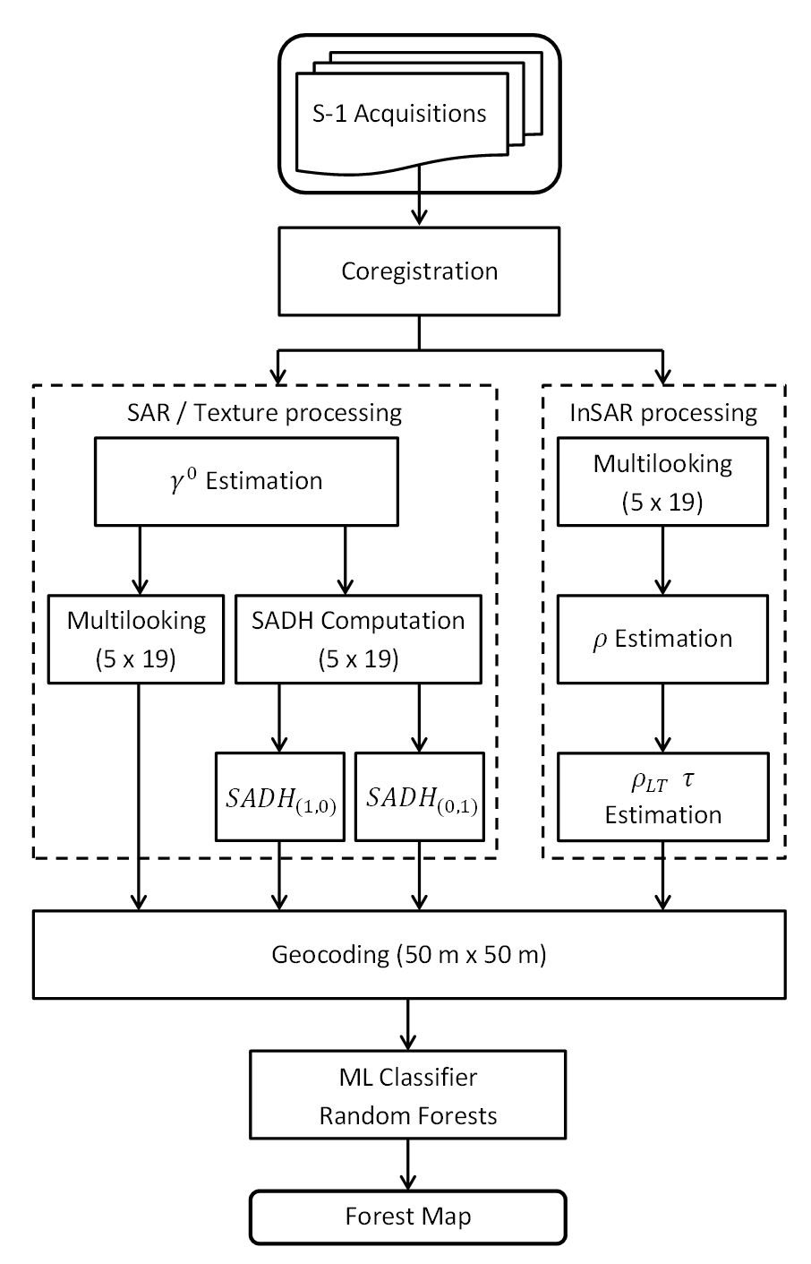
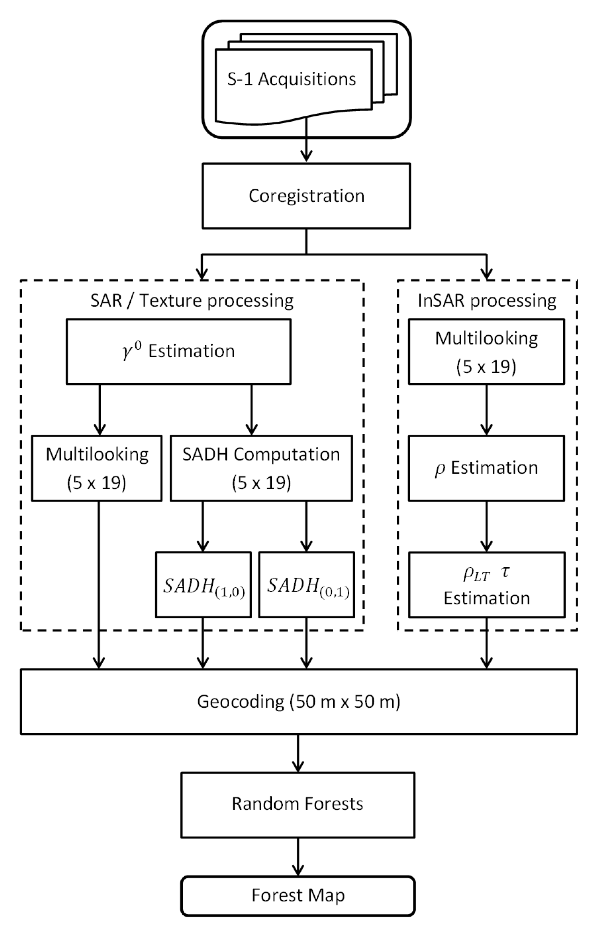
As stated in the introduction, the methodology adopted in our system is based on the one developed in [7], which relies on the use of a monthly interferometric time-series. Figure 1 depicts the new processing chain with the integration of the SADH textures.
The pre-processing steps for the generation of the feature matrices in input to the classifier consist of a coregistration between the interferometric pair followed by an independent analysis of the information retrieved from the radar backscatter and interferometric coherence. As usually done in differential InSAR (DInSAR) applications, all the images in the time-series are coregistered with respect to a common master acquisition, selected as the one in the middle of the temporal stack. Secondly, the backscatter and the coherence from all the possible image pair combinations are estimated by using a moving average filter with a common window size. A boxcar filter with a fixed-size window of pixels was chosen according to:
- the resolution of S-1 IW mode along azimuth and ground range, 14 m × 3.7 m respectively,
- the common goal of having a window centered in the current estimated pixel.
Accordingly, the output resolution is an almost square cell of 70 m × 70.3 m. Regarding the multi-temporal InSAR processing chain, we used the exponential decay model proposed in [7], and recalled in Section 2.1, to fit for each pixel the estimated coherence samples at different temporal baselines. Two key parameters, namely the decorrelation constant and the long-term coherence , are eventually retrieved.
For the backscatter measurement, we consider the projection of the radar brightness on the plane perpendicular to the line of sight, known in literature as the coefficient [21], and we investigate its spatial dependencies in order to extract texture features. On the one hand, we estimated the multi-temporal coefficient by averaging along the temporal dimension and then spatially multi-looking using the same boxcar filter used for the InSAR processing, as suggested in [7]. On the other hand, for the computation of the spatial textures, we considered the multi-temporal mean without applying any spatial multi-looking process. Indeed, at full resolution, the characteristics of different scattering mechanisms can be better preserved. For the application of the SADH method, we set the domain D to pixels and the number of gray levels , in order to obtain a final output resolution which is consistent with the one of the other estimated parameters , , and .
Finally, the feature extraction using the SADH method is repeated twice, considering the most significant displacement vectors along both the azimuth and the slant-range directions. In Figure 1 we named these two set of textures as and , respectively.
After geocoding, all the previously described feature maps are posted to the final resolution of 50 m × 50 m and serve as input to a Random Forests (RF) classifier. As in [7], we considered the Gini index as impurity measurement for the classifier and we set the number of estimators, that is, the number of decision trees, and the minimum number of samples in a leaf node to 50.
Following the branches of the block diagram in Figure 1, a set of S-1 short-time-series can be downloaded and processed, deriving a total of 22 feature maps, 18 textures plus the 4 parameters proposed in [7]. Table 1 summarizes the complete set of features considered in this work.
In Section 5 we present the results of the Random Forests classifier in two different cases, characterized by a different set of input features:
- case (ORIG): , , , and ,
- case (SADH): , , , , , and .
In case (ORIG) we apply the exact algorithm of [7], which represents our baseline. In case (SADH), we additionally use the whole 18 textures extracted from by using the SADH method. In this context, we preliminary measured the Pearson’s correlation coefficient of all the possible combinations of input features and verified that no strong correlated features, either complete decorrelated ones, were present. For this reason, we use all the generated features as input to the Random Forests algorithm.
The comparison between the results is based on the evaluation of the average accuracy () and the overall accuracy () for all the test areas, considering all the valid pixels in the image under test. Given P classes, the associated confusion matrix C assumes in general the following form:
where the elements along the main diagonal, , represent the correctly predicted pixels for each class , that is, they are called class accuracies, and the sum of the elements along each column j corresponds to the number of pixels belonging to each class . The average accuracy defines the mean of each accuracy per single class, that is, the sum of class accuracies divided by the number of classes, while the overall accuracy corresponds to the number of correctly predicted pixels divided by the total number of pixels to predict, that is, the sum of all elements in C. In particular, the respective formulas associated with the two metrics are:
and
While the overall accuracy assesses the global performance of the classifier, the average accuracy further accounts for accuracy unbalancing between the different classes.
4. Materials
The study area covers an extended region over the state of Rondonia, Brazil (approximately 238 thousand km), comprised between and latitude South and and longitude West. This area has become of primary interest, since it is one of the most deforested places in the Amazon basin. Furthermore, since the end of April 2019 the European Space Agency (ESA) has planned a 6-days repeat-pass coverage with the Sentinel-1a and Sentinel-1b satellites in order to monitor the state of the rainforest.
Within this large study area, we downloaded and processed a set of 12 S-1 short-time-series in the framework explained in Figure 1, extracting for each stack the 22 feature maps described in Section 3.
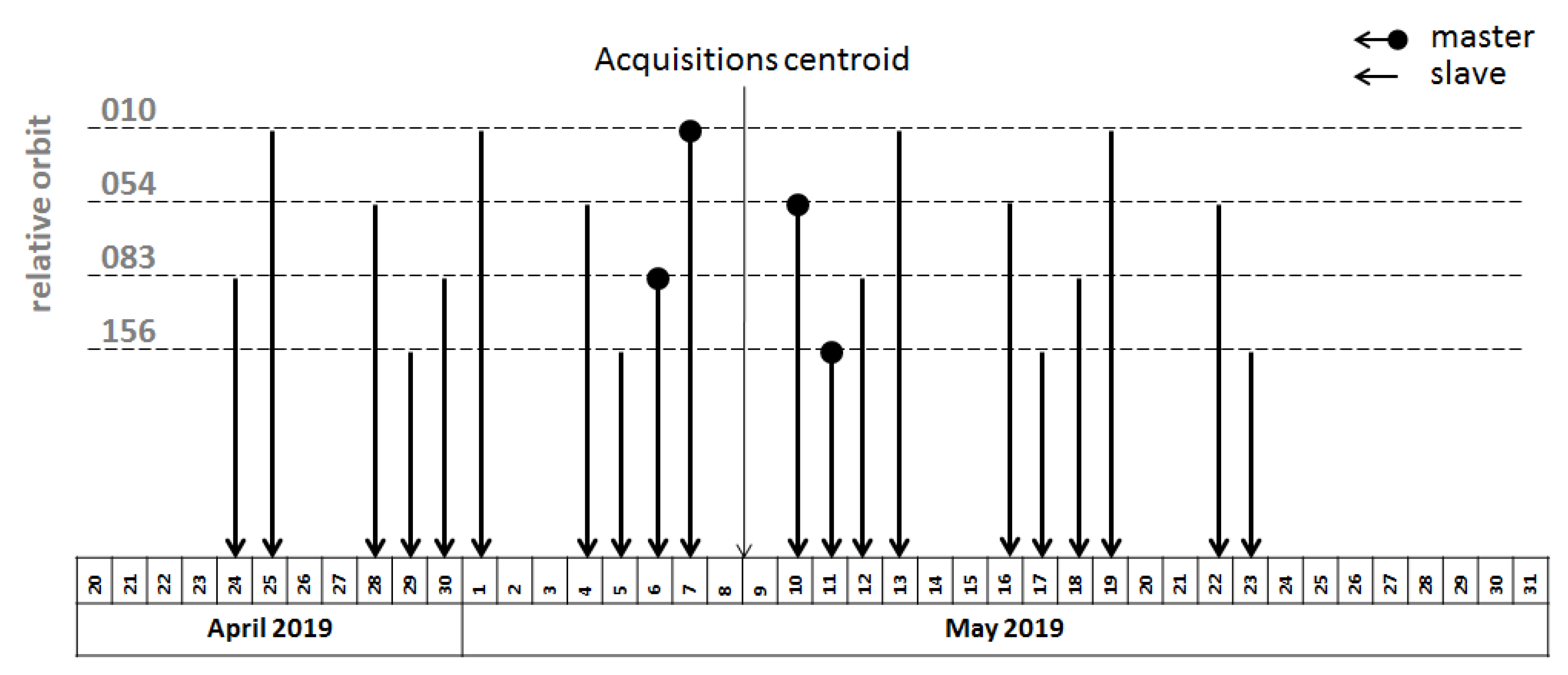
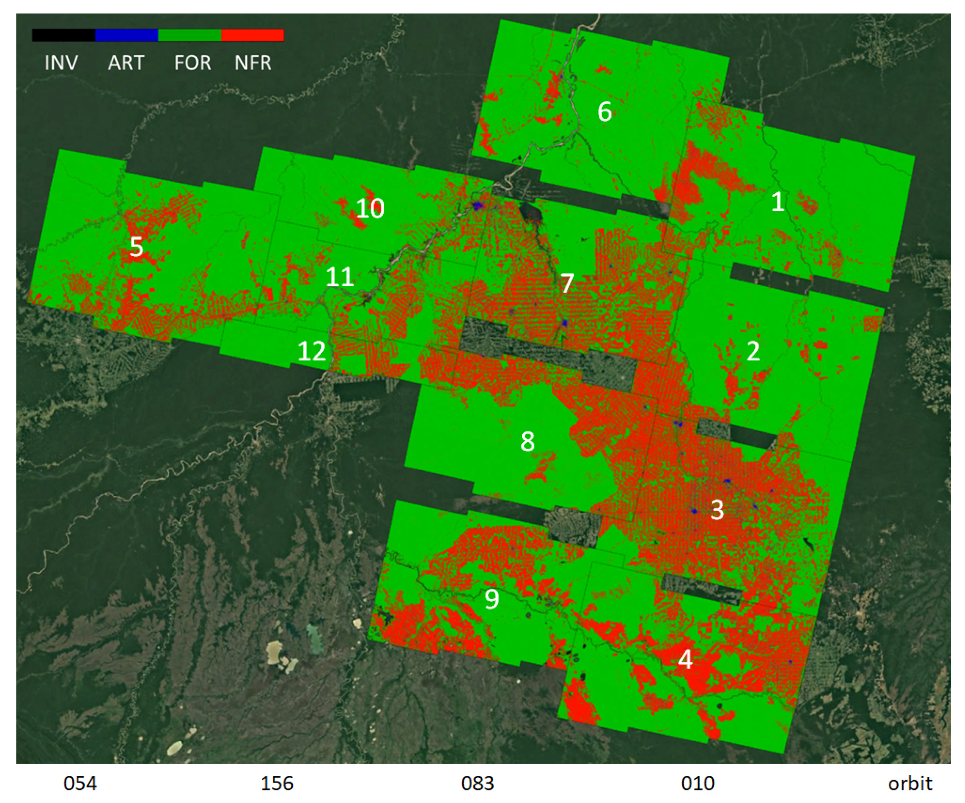
According to Section 3, interferometric stacks of five acquisitions, corresponding to an observation time of 30 days, were coregistered with respect to a master image, chosen as the one in the middle of the acquisitions. As presented in Figure 2 stacks belonging to a certain relative orbit have the same master date and all of these dates are centered around an average date, named acquisitions centroid. The provided 12 common swaths are described in Table 2 and further details can be found in Table A1, while the location of the 12 footprints, superimposed on Google Earth, are depicted in Figure 3. Here, the external reference map FROM-GLC (described in the following) is displayed. From a first visual inspection of Figure 3, some void areas can be identified along the orbit planes. These gaps are due to the misalignment in azimuth between S-1A and S-1B acquisitions and the stringent coregistration requirements for TOPS data. The varying squint (during the acquisition of a burst) causes a large variation of the Doppler centroid within the burst itself and a coregistration error results in a different phase ramp for different bursts, leading to consequently undesired phase jumps between subsequent bursts. In order to ensure a proper coregistration of the data, the enhanced spectral diversity (ESD) technique is applied to the overlapping areas between adjacent bursts [10,22,23]. This approach provides results with accuracy of few centimeters if the overlapping area is sufficiently extended. In correspondence of those gaps this constraint is unfortunately not respected and the interferometric results are therefore not trustworthy.
For both training and validation we used a modified version of the Finer Resolution Observation and Monitoring of Global Land Cover (FROM-GLC) map [24]. This reference is a global land cover map generated using a Random Forests classifier, trained on Landsat Thematic Mapper (TM) and Enhanced Thematic Mapper Plus (ETM+) data and updated to 2017 using additional Sentinel-2 data. Since the FROM-GLC map comprises an inventory of 10 land cover classes, we first grouped them into four macro-classes: artificial surfaces (ART), forests (FOR), non-forested areas (NFR), and water bodies and unclassified or no data as invalids (INV), as shown in Table 3. Secondly, because of the difficulty in finding reliable reference data over the Amazon basin, we discarded all the possible temporal inconsistencies between FROM-GLC reference and Sentinel-1, by relying on the PRODES (Programa de Cálculo do Desflorestamento da Amazônia) digital map [25]. PRODES is a ground polygon inventory derived from visual inspection of optical data and depicts new deforested areas on a yearly base. We therefore extracted from PRODES the polygons corresponding to new cuts occurred between 2017 and 2019 and we set them as invalid samples in the FROM-GLC map, obtaining a more reliable map that, for the sake of simplicity, we named REF. Figure 4 shows the external REF reference map (left), represented as the FROM-GLC 2017 of Figure 3 with in yellow the clearcuts (CUT) marked by PRODES between 2017 and 2019. Those pixels were grouped to the class invalids (INV), then, discarded in both the training and the validation.
Moreover, a further analysis by means of high-resolution multi-spectral Sentinel-2 (S-2) data is presented in Section 5. In order to avoid unwanted effects caused by the presence of clouds, we selected the best S-2 acquisition within the analyzed time span accordingly to the past weather information [26]. From a visual inspection and a check of the cloud shadow mask available in the Level 2A product, we considered the acquisitions on the 16 May 2019 as the most reliable one.
5. Results
The experiments were conducted by splitting the twelve stacks of Table 2 into validation and training swaths. The former were selected in order to cover a strip of about 250 km × 1000 km crossing the Rondonia state, as shown in Figure 4, and they correspond to the stacks of the relative orbit 83, marked with asterisks in Table 2. The other swaths were chosen for training the Random Forests algorithm: in particular, we selected 5 million pixels for each of the considered classes. According to the Random Forests common issues for the training stage [27], these samples were randomly selected from all the training swaths, with the exception of the pixels of the class ART, artificially replicated because of the poor data availability. In this way, we were able to generate a well-balanced training data set. In this paper, we first concentrate on the algorithm performance assessment over a large-scale area located along the S-1 relative orbit plane number 83, and, more specifically, comprising stacks 6, 7, 8, and 9 in Table 2. Secondly, we analyze four significant patches of pixels, selected within the swath corresponding to stack 7 in Table 2.
5.1. Large-Scale Classification
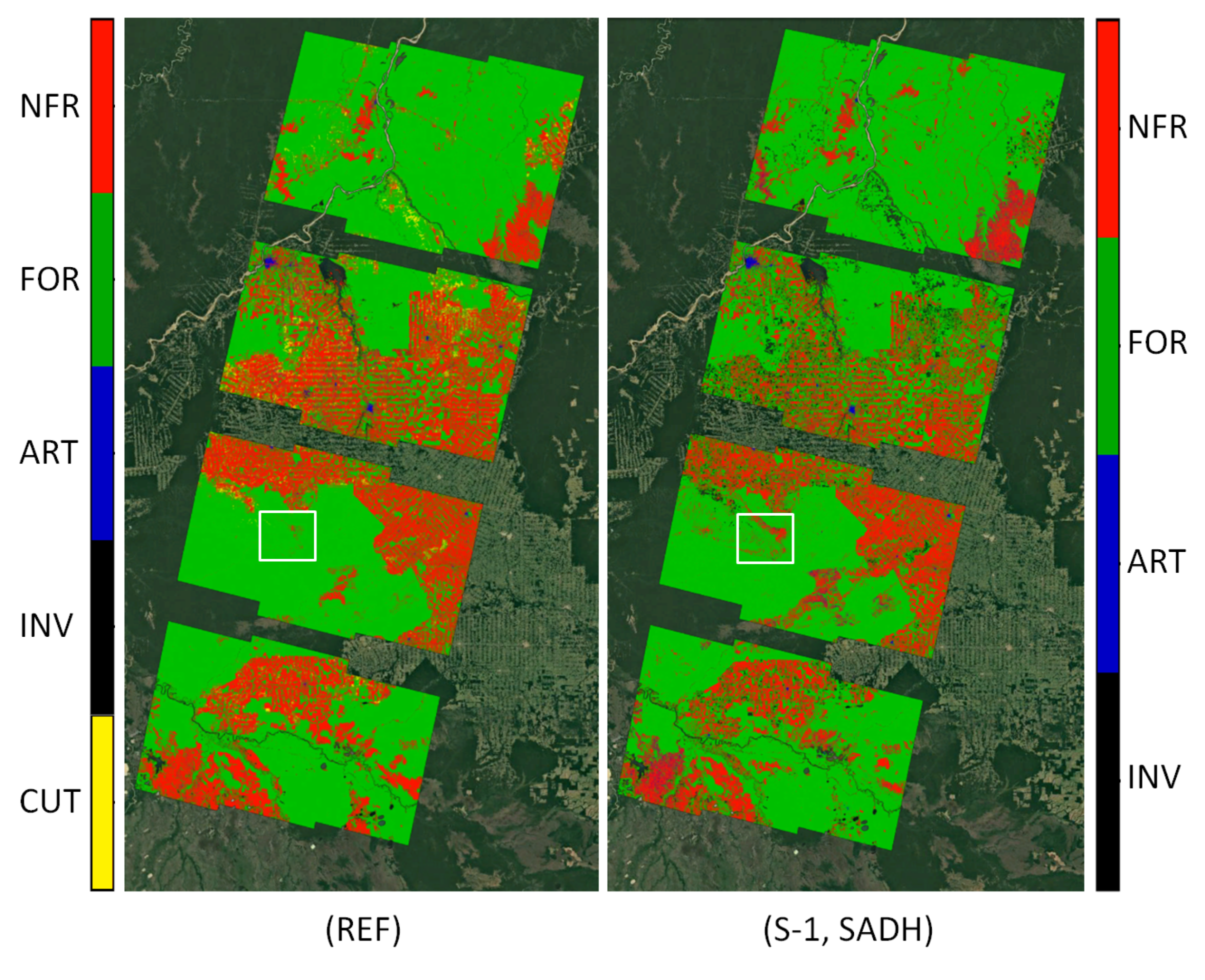
In this first analysis we concentrate on the results obtained by applying the proposed algorithm to the large-scale area shown in Figure 4, where a comparison between the REF reference map and case (SADH) for the four swaths acquired with orbit number 83 is presented. The performance analysis is carried out using both the overall and average accuracy parameters denoted as OA and AA, respectively, and Table 4 summarizes the two metrics for each of the four stacks, considering the set of inputs in case (ORIG) and in case (SADH).
5.2. Analysis of Single Patches
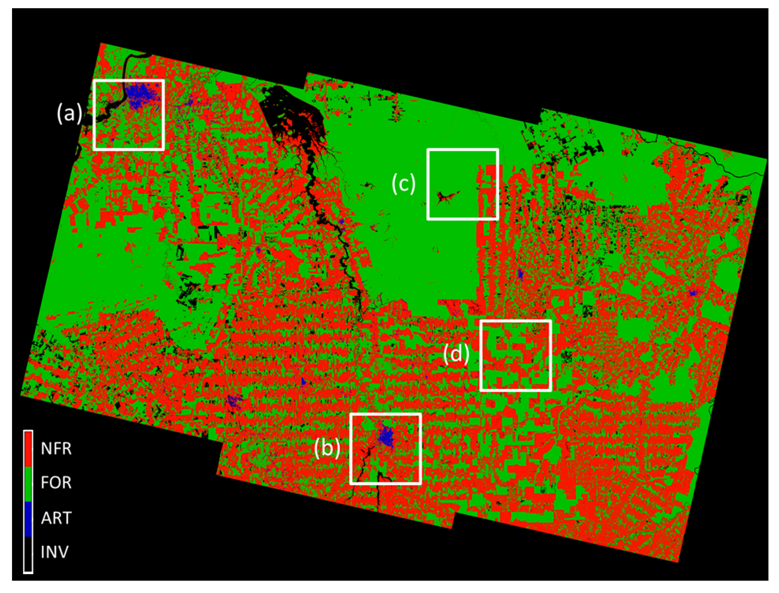
In the following we consider the S-1 swath corresponding to stack 7 in Table 2 and we provide a performance analysis of our proposed algorithm over selected patches, in order to analyze specific details in the images. As shown in Figure 5, we select four small patches of pixels, extending by about 25 km × 25 km on ground. Patches (a) and (b) are characterized by the presence of urban areas, that is, the municipalities of Porto Velho and Ariquemes, respectively, while patches (c) and (d) identify stable regions of cropland mixed with remaining rainforest areas. Similarly to Section 5.1, we summarize the results of the patches in Figure 6 and Table 5, which describes the OA and AA for each patch, in both the input configurations, case (ORIG) and case (SADH).
6. Discussion
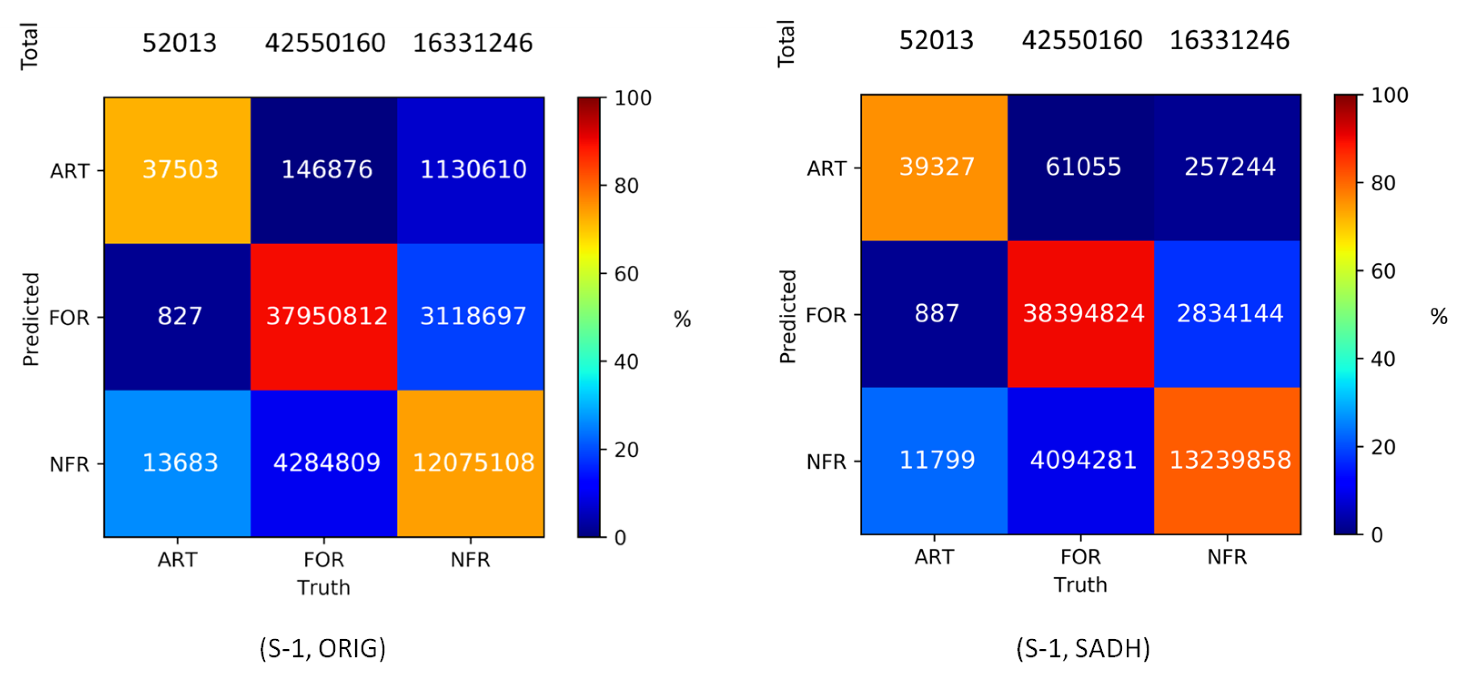
In this section, the experimental results presented in Section 5 are discussed in the same order, starting from the large-scale classification analysis of Section 5.1. In Table 4 all considered swaths are characterized by an overall accuracy above 82.50% and 84.26% for the (ORIG) and (SADH) cases, respectively, by considering all valid pixels within the images. Again, the additional information of the SADH textures increases both the OA and the AA of at least 1.5% in all four swaths. In particular, the use of the SADH textures allows the Random Forests to improve the detection performance, especially for the ART and NFR classes, depicted in blue and red, respectively, in Figure 4 and better visible with the analysis of the global confusion matrices in Figure 7.
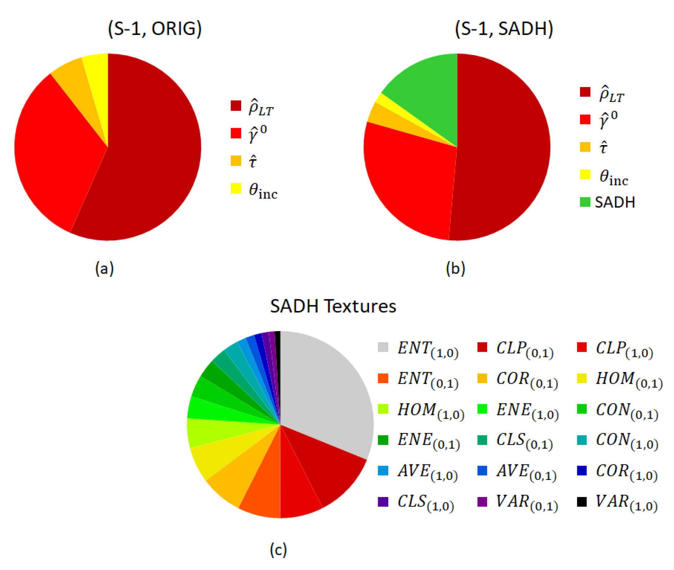
Figure 8 shows the pie charts related to the feature importance in the two considered cases ORIG (a) and SADH (b) by grouping all the texture features together. We notice that the set of texture features has quite a strong relevance in the Random Forests prediction and improves the classification accuracy presented in Table 4. Furthermore, in Figure 8c we show how the features importance is distributed for the 18 SADH textures only, partitioning the green slice of the pie chart in Figure 8b only. Here we can see how the entropy (ENT) plays a key role among all other features, while the less informative is the pure variance (VAR).
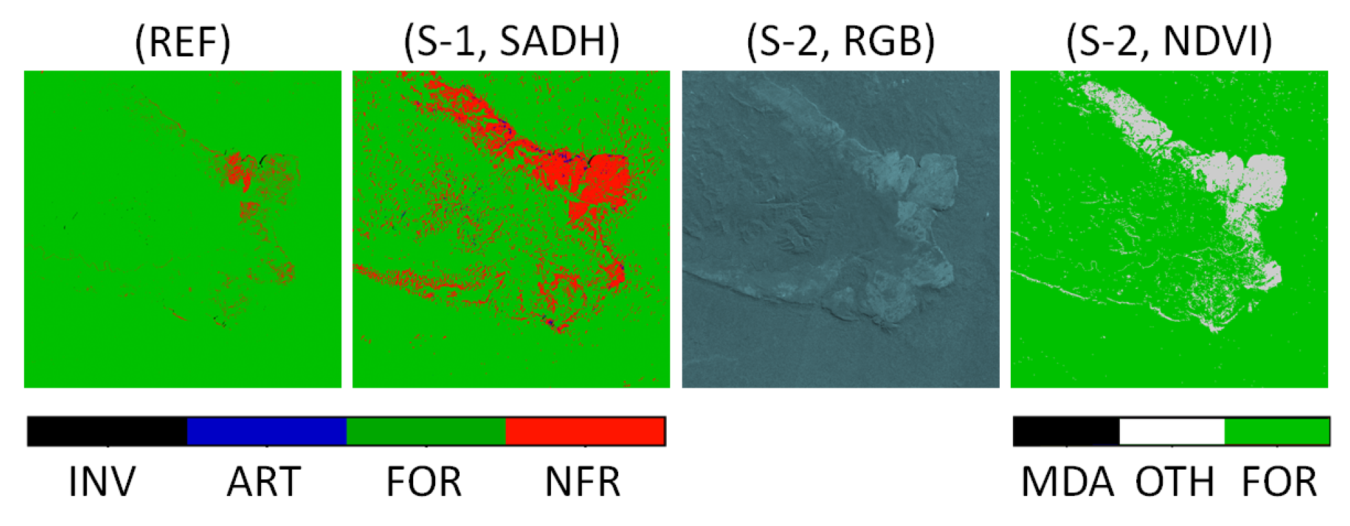
Moreover, during the investigation, we noted that an additional source of inconsistency between the reference and the resulting classification map is given by the different semantic interpretation of radar and optical sensors over some areas characterized by the presence of rough terrain and sparse vegetation. As an example, we analyze the white patch in Figure 4, of size pixels, corresponding to a portion of stack 8 in Table 2. It corresponds to an area of the Pacaás Novos National Park. As reported in the corresponding S-2 RGB map of Figure 9 that area comprises a plateau with a peak in the upper-right side of the patch, called mount Tracoa. Through a visual comparison between the NDVI and RGB maps, retrieved from the S-2 acquisition of 2019, and the REF reference of 2017, it is now clear that the latter is not really sensitive to the presence of low and sparse vegetation. On the other hand, the result obtained from case (SADH) clearly show the same patterns visible within the optical data. The reader should therefore be aware that these kinds of discrepancies, even if they actually represent a source of information, might slightly decrease the computed performance of the proposed methodology, calculated by considering the REF only as external reference map.
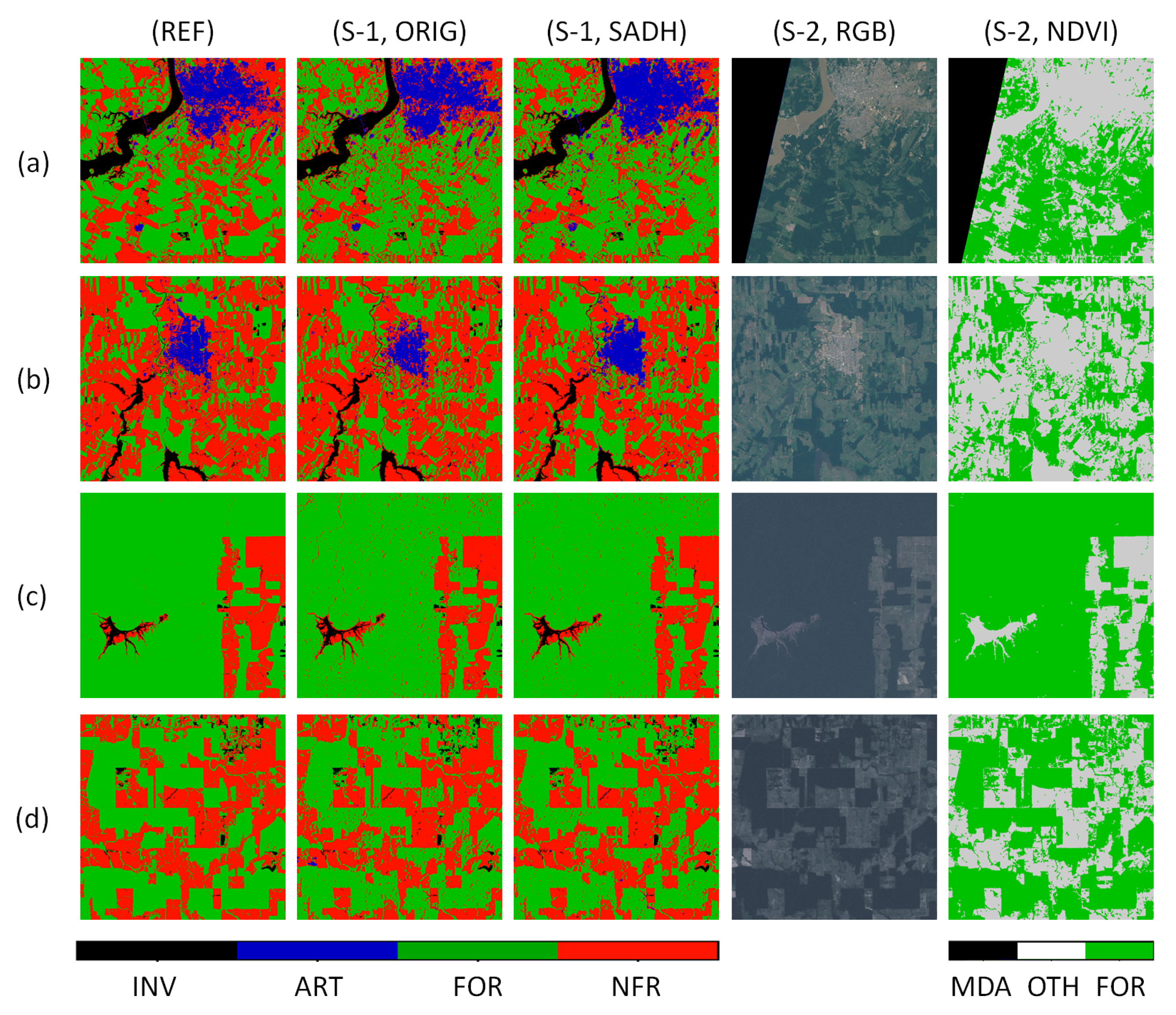
By observing the REF reference and the results of case (ORIG) and case (SADH) in Figure 6, it can be seen how the introduction of the texture information in case (SADH) helps improving the classification with respect to case (ORIG), by better isolating urban areas and closing gaps over forested areas. This is confirmed by the corresponding accuracy values in Table 5, where a positive increment of both the overall and average accuracy, and , respectively, is detected. In particular, in patches (a) and (b), textures are helpful to better classify small details in man-made structures. This results in a slight increase of the overall accuracy (between 1.29% and 1.78%), together with a more relevant improvement in the average accuracy as well (between 2.21% and 6.02%). In patch (c), the inclusion of SADH textures provides a better segmentation of the class forests (FOR) with respect to the classification results obtained using the sole interferometric and backscattering parameters. The random noise-like misclassification occurrencies are reduced, resulting in an increase of both OA and AA, which varies between 1.12% and 2.10%. Finally, in patch (d) the introduction of textures also allows for correctly classifying bare soil areas as non-forested areas (NFR), which would otherwise result in misclassified artificial surfaces (ART).
As a further comment, although this first analysis demonstrates the improvement obtained by using the SADH textures for all the considered patches, patch (a) presents lower values of accuracy with respect to the other ones even when considering case (SADH), with an overall and average accuracy of 73.60% and 78.15%, respectively. Such low values are mainly caused by the time difference between the Sentinel-1 acquisitions (April–May 2019) and the REF reference map from 2017. Indeed, this is confirmed by observing the True Color (RGB) and the Normalized Difference Vegetation Index (NDVI) maps from a Sentinel-2 acquisition of 16 May 2019, depicted in the last two columns of Figure 6. The RGB map shows how the city of Porto Velho, the capital of Rondonia, is more extended with respect to 2017, especially on the top-right corner of patch (a). Similar inconsistencies can also be found in patch (b) when observing both the urban and the deforested areas. For example, with respect to the reference REF map, a squared re-vegetated area can be detected at the top-left corner of patch (b), whose presence is again confirmed by the NDVI index extracted from the Sentinel-2 acquisition of 2019.
7. Conclusions
The work that we presented in this paper demonstrates the high potential of multi-temporal interferometric short-time-series for forest mapping purposes and, in particular, for an effective monitoring of the Amazon rainforest. By combining the information retrieved from backscatter, together with temporal interferometric parameters and spatial textures, it is possible to produce accurate large-scale forest maps at regular intervals. In particular, the introduction of backscatter spatial textures, with respect to the previous stand of the technique, allows for the achievement of a consistent improvement of the final classification accuracy at the cost of a moderate increase of computational effort thanks to the SADH method implementation. The use of backscatter spatial textures significantly improves the correct discrimination between non-forested areas and artificial surfaces.
As case study, we selected an area over the Rondonia State, Brazil, characterized by the availability of six-days repeat-pass Sentinel-1 interferometric time-series, acquired over an overall period of 30 days only (short-time-series), achieving accuracy values always above 80%. It is worth noting that some inconsistencies between the obtained results and the external reference map are not due to effective misclassification, but to the different acquisition time frame between the generated maps and the external reference. This is confirmed by the additional analysis of Sentinel-2 optical data, acquired during the same time span.
The proposed methodology sets the basis for the development of an operational framework for the effective monitoring of forest changes at a monthly rate, by performing change detection between subsequent multi-temporal stacks. This last aspect is of great interest for the development of an early-warning system, which could effectively support the deputy authorities to identify illegal deforestation hot-spots and therefore protect the rainforest resources.
Author Contributions
Conceptualization, A.P., F.S., R.A.S. and P.R.; methodology, A.P., F.S., R.A.S. and P.R.; software, A.P., and R.A.S.; validation, A.P.; investigation, A.P.; data curation, A.P., F.S., P.P. and P.R.; writing–original draft preparation, A.P.; writing–review and editing, F.S. and P.R.; supervision, F.S. and P.R. All authors have read and agreed to the published version of the manuscript.
Funding
This research was partially funded through the HI-FIVE project, granted by the ESA Living Planet Fellowship 2018.
Acknowledgments
The authors gratefully acknowledge the contribution by Diego Fernández-Prieto in supporting the acquisition plan of Sentinel-1 over the state of Rondonia.
Conflicts of Interest
The authors declare no conflict of interest.
Appendix A

Table A1.
Ancillary information about the Sentinel-1 acquisitions selected for the 12 short-time-series.
Table A1.
Ancillary information about the Sentinel-1 acquisitions selected for the 12 short-time-series.
| List of Acquisitions | |||||||||
|---|---|---|---|---|---|---|---|---|---|
| Name | |||||||||
| Orbit | Date | Sensor | Mode | Type | Level | ID | ID | ID | ID |
| 2019.04.25 | S1B | IW | SLC | 1 | 432C | 4D3E | 416E | A798 | |
| 2019.05.01 | S1A | IW | SLC | 1 | 7E8C | 93EC | F1D1 | 744F | |
| 010 | 2019.05.07 | S1B | IW | SLC | 1 | E44A | F86E | E876 | EBCE |
| 2019.05.13 | S1A | IW | SLC | 1 | 5D14 | 7F74 | 1105 | CD19 | |
| 2019.05.19 | S1B | IW | SLC | 1 | 5239 | F6E8 | D8E8 | 148C | |
| Stack | 1 | 2 | 3 | 4 | |||||
| Name | |||||||||
| Orbit | Date | Sensor | Mode | Type | Level | ID | ID | ID | ID |
| 2019.04.28 | S1B | IW | SLC | 1 | 1E1A | ||||
| 2019.05.04 | S1A | IW | SLC | 1 | 036E | ||||
| 054 | 2019.05.10 | S1B | IW | SLC | 1 | E759 | |||
| 2019.05.16 | S1A | IW | SLC | 1 | 4387 | ||||
| 2019.05.22 | S1B | IW | SLC | 1 | 6425 | ||||
| Stack | 5 | ||||||||
| Name | |||||||||
| Orbit | Date | Sensor | Mode | Type | Level | ID | ID | ID | ID |
| 2019.04.24 | S1A | IW | SLC | 1 | 3540 | D975 | 4377 | 16C4 | |
| 2019.04.30 | S1B | IW | SLC | 1 | 15A6 | C128 | DB79 | F212 | |
| 083 | 2019.05.06 | S1A | IW | SLC | 1 | 7107 | FEBF | 19E1 | 1048 |
| 2019.05.12 | S1B | IW | SLC | 1 | 1564 | 24AE | E331 | 430E | |
| 2019.05.18 | S1A | IW | SLC | 1 | 8EBB | 93C1 | 6547 | A78A | |
| Stack | 6 | 7 | 8 | 9 | |||||
| Name | |||||||||
| Orbit | Date | Sensor | Mode | Type | Level | ID | ID | ID | ID |
| 2019.04.29 | S1A | IW | SLC | 1 | 831D | F0E2 | F0E2 | ||
| 2019.05.05 | S1B | IW | SLC | 1 | 2C50 | 2C50 | 5973 | ||
| 156 | 2019.05.11 | S1A | IW | SLC | 1 | B4E4 | 1AE8 | 1AE8 | |
| 2019.05.17 | S1B | IW | SLC | 1 | AEED | AEED | 8239 | ||
| 2019.05.23 | S1A | IW | SLC | 1 | E7BE | 0B54 | 0B54 | ||
| Stack | 10 | 11 | 12 | ||||||
References
- Bonan, G. Ecological Climatology: Concepts and Applications, 3rd ed.; Cambridge University Press: Cambridge, UK, 2015. [Google Scholar]
- Blouet, B.W.; Blouet, O.M. Latin America and the Caribbean: A Systematic and Regional Survey, 7th ed.; Wiley: Hoboken, NJ, USA, 2015. [Google Scholar]
- Marengo, J. On the hydrological cycle of the Amazon Basin: A historical review and current state-of-the-art. Revista Brasileira de Meteorologia 2006, 21, 1–19. [Google Scholar]
- Baer, H.; Singer, M. The Anthropology of Climate Change: An Integrated Critical Perspective, 1st ed.; Routledge: Abingdon, UK, 2014. [Google Scholar]
- Shimada, M.; Itoh, T.; Motooka, T.; Watanabe, M.; Shiraishi, T.; Thapa, R.; Lucas, R. New global forest/non-forest maps from ALOS PALSAR data (2007–2010). Remote Sens. Environ. 2014, 155, 13–31. [Google Scholar] [CrossRef]
- Martone, M.; Rizzoli, P.; Wecklich, C.; Gonzalez, C.; Bueso-Bello, J.L.; Valdo, P.; Schulze, D.; Zink, M.; Krieger, G.; Moreira, A. The global forest/non-forest map from TanDEM-X interferometric SAR data. Remote Sens. Environ. 2018, 205, 352–373. [Google Scholar] [CrossRef]
- Sica, F.; Pulella, A.; Nannini, M.; Pinheiro, M.; Rizzoli, P. Repeat-pass SAR interferometry for land cover classification: A methodology using Sentinel-1 Short-Time-Series. Remote Sens. Environ. 2019, 232, 111277. [Google Scholar] [CrossRef]
- Torres, R.; Snoeij, P.; Geudtner, D.; Bibby, D.; Davidson, M.; Attema, E.; Potin, P.; Rommen, B.; Floury, N.; Brown, M.; et al. GMES Sentinel-1 mission. Remote Sens. Environ. 2012, 120, 9–24. [Google Scholar] [CrossRef]
- De Zan, F.; Monti-Guarnieri, A. TOPSAR: Terrain observation by progressive scans. IEEE Trans. Geosci. Remote Sens. 2006, 44, 2352–2360. [Google Scholar] [CrossRef]
- Yague-Martinez, N.; Prats-Iraola, P.; Gonzalez, F.; Brcic, R.; Shau, R.; Geudtner, D.; Eineder, M.; Bamler, R. Interferometric Processing of Sentinel-1 TOPS Data. IEEE Trans. Geosci. Remote Sens. 2016, 54, 1–15. [Google Scholar] [CrossRef] [Green Version]
- Rocca, F. Modeling interferogram stacks. IEEE Trans. Geosci. Remote Sens. 2007, 45, 3289–3299. [Google Scholar] [CrossRef]
- Krieger, G.; Moreira, A.; Fiedler, H.; Hajnsek, I.; Werner, M.; Younis, M.; Zink, M. TanDEM-X: A satellite formation for high-resolution SAR interferometry. IEEE Trans. Geosci. Remote Sens. 2007, 45, 3317–3341. [Google Scholar] [CrossRef] [Green Version]
- Parizzi, A.; Cong, X.Y.; Eineder, M. First Results from Multifrequency Interferometry. A Comparison of Different Decorrelation Time Constants at L, C and X Band; ESA Special Publication; ESA: Paris, France, 2010; Volume 677. [Google Scholar]
- Bruzzone, L.; Marconcini, M.; Wegmuller, U.; Wiesmann, A. An Advanced System for the Automatic Classification of Multitemporal SAR Images. IEEE Trans. Geosci. Remote Sens. 2004, 42, 1321–1334. [Google Scholar] [CrossRef]
- Tuceryan, M.; Jain, A.K. Texture analysis. In The Handbook of Pattern Recognition and Computer Vision, 2nd ed.; World Scientific Publishing C.: Singapore, 1998; pp. 207–248. [Google Scholar]
- Kuplich, T.M.; Curran, P.J.; Atkinson, P.M. Relating SAR image texture and backscatter to tropical forest biomass. In Proceedings of the IEEE International Geoscience and Remote Sensing Symposium (IGARSS2003), Toulouse, France, 21–25 July 2003; IEEE: Hoboken, NJ, USA, 2003; Volume 4, pp. 2872–2874. [Google Scholar]
- Dekker, R.J. Texture Analysis and Classification of ERS SAR Images for Map Updating of Urban Areas in The Netherlands. IEEE Trans. Geosci. Remote Sens. 2003, 41, 1950–1958. [Google Scholar] [CrossRef]
- Unser, M. Sum and difference histograms for texture classification. IEEE Trans. Pattern Anal. Mach. Intell. 1986, PAMI-8, 118–125. [Google Scholar] [CrossRef] [PubMed]
- Haralick, R.M.; Shanmugam, K.; Dinstein, I. Textural Features for Image Classification. IEEE Trans. Syst. Man Cybern. 1973, SMC-3, 610–621. [Google Scholar] [CrossRef] [Green Version]
- Haralick, R.M. Statistical and structural approaches to texture. IEEE Proc. 1979, 67, 786–804. [Google Scholar] [CrossRef]
- Small, D. Flattening gamma: Radiometric terrain correction for SAR imagery. IEEE Trans. Geosci. Remote Sens. 2011, 49, 3018–3093. [Google Scholar] [CrossRef]
- Prats-Iraola, P.; Scheiber, R.; Marotti, L.; Wollstadt, S.; Reigber, A. TOPS interferometry with TerraSAR-X. IEEE Trans. Geosci. Remote Sens. 2012, 50, 3179–3188. [Google Scholar] [CrossRef] [Green Version]
- Nannini, M.; Prats-Iraola, P.; Scheiber, R.; Yague-Martinez, N.; Minati, F.; Vecchioli, F.; Costantini, M.; Borgstrom, S.; de Martino, P.; Siniscalchi, V.; et al. Sentinel-1 mission: Results of the InSARap project. In Proceedings of the VDE 11th European Conference on Synthetic Aperture Radar (EUSAR2016), Hamburg, Germany, 6–9 June 2016; IEEE: Hoboken, NJ, USA, 2016; pp. 1–4. [Google Scholar]
- Gong, P.; Liu, H.; Zhang, M.; Li, C.; Wang, J.; Huang, H.; Clinton, N.; Ji, L.; Li, W.; Bai, Y.; et al. Stable classification with limited sample: Transferring a 30-m resolution sample set collected in 2015 to mapping 10-m resolution global land cover in 2017. Sci. Bull. 2019, 64, 370–373. [Google Scholar] [CrossRef] [Green Version]
- Valeriano, D.M.; Mello, E.M.K.; Moreira, J.C.; Shimabukuro, Y.E.; Duarte, V.; Souza, I.M.; dos Santos, J.R.; Barbosa, C.C.F.; de Souza, R.C.M. Monitoring tropical forest from space: The prodes digital project. Int. Arch. Photogramm. Remote. Sens. Spat. Inf. Sci. 2004, 35, 272–274. [Google Scholar]
- Past Weather in Porto Velho, Rondônia, Brazil—May 2019. Available online: https://www.timeanddate.com/weather/brazil/porto-velho/historic?month=5&year=2019 (accessed on 20 January 2020).
- Breiman, L. Random Forests. Mach. Learning 2001, 45, 5–32. [Google Scholar] [CrossRef] [Green Version]
Figure 1.
Developed processing chain for short-time-series, based on the architecture presented in [7], with the integration of Sum and Difference Histograms (SADH) textures.
Figure 1.
Developed processing chain for short-time-series, based on the architecture presented in [7], with the integration of Sum and Difference Histograms (SADH) textures.

Figure 2.
Sentinel-1 acquisition times description. A dot represents the master image, while the arrows represent the date of the slave images. The acquisitions centroid represents the average date among all the master acquisitions.
Figure 2.
Sentinel-1 acquisition times description. A dot represents the master image, while the arrows represent the date of the slave images. The acquisitions centroid represents the average date among all the master acquisitions.

Figure 3.
Finer Resolution Observation and Monitoring of Global Land Cover (FROM-GLC, 2017) reference map chosen for the training and validation stages. Black: invalid pixels (INV), blue: artificial surfaces (ART), green: forests (FOR), red: non-forested areas (NFR). The white numbers identify the corresponding stack, described in Table 2, while the numbers at the bottom show the orbits associated to the different swaths.

Figure 4.
Comparison between the REF reference (left), with in yellow the clearcuts (CUT) marked by PRODES between 2017 and 2019, and the final result of the Random Forests algorithm using SADH textures (right). The white square identifies a region of interest in which the maps are clearly different. Such an area corresponds to the Pacaás Novos National Park and is separately analyzed in Figure 9.

Figure 5.
Classification map of the stack number 7 summarized in Table 2. Black: invalid pixels (INV), blue: artificial surfaces (ART), green: forests (FOR), red: non-forested areas (NFR). White polygons delimit four patches of pixels used for the classification accuracy analysis. They are named (a), (b), (c), and (d).

Figure 6.
Four analyzed patches of pixels are placed along the rows. They are indicated as (a–d), selected from the classification results over the stack number 7 defined in Table 2. Each column addresses to a different quantity: (REF) is the modified FROM-GLC reference with the clearcuts marked by PRODES between 2017 and 2019 as invalids (INV), (S-1, ORIG) is the Random Forests classification map using the input parameters from [7] only, (S-1, SADH) is the Random Forests result adding the SADH textures to the original parameters, (S-2, RGB) and (S-2, NDVI) are the optical True Color and NDVI maps, respectively, of Sentinel-2 acquisitions from the considered month. (REF), (S-1, ORIG), and (S-1, SADH) maps follow the legend described in Figure 5, while (S-2, NDVI) map comprises three classes: missing data (MDA) in black, forests (FOR) in green, and other structures (OTH) in white.

Figure 7.
Confusion matrices for the whole test dataset, considering the two analyzed cases, (ORIG) and (SADH). The sum of all the elements along each column correspond to the total number of pixels associated to each class. The elements along the diagonal of the confusion matrix correspond to the correctly predicted pixels, class-by-class. The color associated to each element corresponds to the percentage obtained by normalizing the current element for the total number of samples for each specific class.

Figure 8.
Feature importance for the two analyzed cases, (a) ORIG and (b) SADH; in particular, pie chart (c) shows the distribution of importance for the SADH textures only.
Figure 8.
Feature importance for the two analyzed cases, (a) ORIG and (b) SADH; in particular, pie chart (c) shows the distribution of importance for the SADH textures only.

Figure 9.
Comparison between, from left to right, the selected reference (REF), the final result of the Random Forests algorithm (S-1, SADH) and the True Color (S-2, RGB) and NDVI (S-2, NDVI) map extracted from the best Sentinel-2 acquisition within the same observation month. The analyzed pixels patch corresponds to an area located around the mount Tracoa, in the Pacaás Novos National Park, Rondonia State, Brazil.

Table 1.
List of the 22 features considered in Section 5. Column shows the parameters used in [7], while columns and explain the textures extracted by using displacement vectors along both the azimuth and the slant-range directions, respectively, whose mathematical formulation is presented in Equations (4)–(12).
Table 2.
Sentinel-1 stacks description. From left to right: stack number, relative orbit number, name of the time-series associated to the orbit number, corner coordinates in latitude (Lat. min and Lat. max) and longitude (Lon. min and Lon. max). The stacks marked with an asterisk are chosen for the validation, while the others are used for training the Random Forests algorithm.
| Corner Coordinates [deg] | ||||||
|---|---|---|---|---|---|---|
| Stack | Orbit | Name | Lat. Min | Lat. Max | Lon. Min | Lon. Max |
| 1 | 010 | |||||
| 2 | 010 | |||||
| 3 | 010 | |||||
| 4 | 010 | |||||
| 5 | 054 | |||||
| 6* | 083 | |||||
| 7* | 083 | |||||
| 8* | 083 | |||||
| 9* | 083 | |||||
| 10 | 156 | |||||
| 11 | 156 | |||||
| 12 | 156 | |||||
Table 3.
Finer Resolution Observation and Monitoring of Global Land Cover (FROM-GLC) classes aggregation strategy: artificial surfaces (ART), forests (FOR), non-forested areas (NFR), and water bodies and unclassified or no data as invalids (INV).
Table 3.
Finer Resolution Observation and Monitoring of Global Land Cover (FROM-GLC) classes aggregation strategy: artificial surfaces (ART), forests (FOR), non-forested areas (NFR), and water bodies and unclassified or no data as invalids (INV).
| FROM-GLC | Higher-Level Class |
|---|---|
| Unclassified | |
| Water | INV |
| Snow/Ice | |
| Impervious surface | ART |
| Forest | FOR |
| Cropland | NFR |
| Grassland | |
| Shrubland | |
| Wetland | |
| Tundra | |
| Bareland |
Table 4.
Overall accuracy (OA) and average accuracy (AA) for the four swaths in Figure 4. Each swath is associated to a stack, according to the enumeration in Table 2.
| Class | Stack 6 | Stack 7 | Stack 8 | Stack 9 | |
|---|---|---|---|---|---|
| ART | 10060 | 34890 | 6009 | 1054 | |
| pixels | FOR | 14626324 | 7846234 | 9822268 | 10087671 |
| NFR | 1655335 | 6194973 | 4193972 | 4280135 | |
| Case | Metric | Stack 6 | Stack 7 | Stack 8 | Stack 9 |
| ORIG | OA | 88.48% | 82.50% | 85.03% | 84.84% |
| AA | 61.05% | 81.64% | 80.50% | 71.95% | |
| SADH | OA | 91.90% | 84.26% | 86.49% | 87.66% |
| AA | 65.11% | 85.59% | 85.06% | 82.46% |
Table 5.
Overall accuracy (OA) and average accuracy (AA) for the four patches in Figure 6: patch (a) and patch (b) are characterized by urban areas, while patch (c) and patch (d) contain clear-cuts. and represent the increment in (OA) and (AA), respectively, when including textures within the classification.
| Class | Patch (a) | Patch (b) | Patch (c) | Patch (d) | |
|---|---|---|---|---|---|
| ART | 20419 | 7706 | 0 | 0 | |
| pixels | FOR | 118922 | 86290 | 216741 | 141669 |
| NFR | 100506 | 155408 | 42073 | 117044 | |
| Case | Metric | Patch (a) | Patch (b) | Patch (c) | Patch (d) |
| ORIG | OA | 72.31% | 80.71% | 94.63% | 85.88% |
| AA | 75.94% | 79.96% | 93.04% | 85.79% | |
| SADH | OA | 73.60% | 82.49% | 95.75% | 87.98% |
| AA | 78.15% | 85.98% | 94.28% | 87.88% | |
| 1.29% | 1.78% | 1.12% | 2.10% | ||
| 2.21% | 6.02% | 1.24% | 2.09% |
© 2020 by the authors. Licensee MDPI, Basel, Switzerland. This article is an open access article distributed under the terms and conditions of the Creative Commons Attribution (CC BY) license (http://creativecommons.org/licenses/by/4.0/).
Share and Cite
MDPI and ACS Style
Pulella, A.; Aragão Santos, R.; Sica, F.; Posovszky, P.; Rizzoli, P. Multi-Temporal Sentinel-1 Backscatter and Coherence for Rainforest Mapping. Remote Sens. 2020, 12, 847. https://doi.org/10.3390/rs12050847
AMA Style
Pulella A, Aragão Santos R, Sica F, Posovszky P, Rizzoli P. Multi-Temporal Sentinel-1 Backscatter and Coherence for Rainforest Mapping. Remote Sensing. 2020; 12(5):847. https://doi.org/10.3390/rs12050847
Chicago/Turabian StylePulella, Andrea, Rodrigo Aragão Santos, Francescopaolo Sica, Philipp Posovszky, and Paola Rizzoli. 2020. "Multi-Temporal Sentinel-1 Backscatter and Coherence for Rainforest Mapping" Remote Sensing 12, no. 5: 847. https://doi.org/10.3390/rs12050847
Note that from the first issue of 2016, this journal uses article numbers instead of page numbers. See further details here.