Seasonal and Interannual Variations in China’s Groundwater Based on GRACE Data and Multisource Hydrological Models

Abstract

In this study, we used in situ measurements for the first time to analyze the applicability and effectiveness of evaluating groundwater storage (GWS) changes across China using Gravity Recovery and Climate Experiment (GRACE) satellite products and hydrological data derived from the WaterGap Global Hydrological Model (WGHM), Global Land Data Assimilation System (GLDAS) and eartH2Observe (E2O). The results show that the GWS derived from GRACE JPL Mascons products combined with GLDAS Noah V2.1 data most accurately reflect the overall distribution of GWS changes in China and the correlation coefficient between the in situ measurements reaches 0.538. The empirical orthogonal function decomposition for GWS indicates clear interannual variation and seasonal variation in China. The trends of China’s GWS changes showed a clear regional characteristic from 2003 to 2016. The GWS in the northeast, central-south, and western junction of Xinjiang-Qinghai-Tibet had increased significantly, and the North China Plain (NCP) had a severe decline. The correlation coefficient between the annual trends of precipitation and GWS was 0.57, and it reached 0.73 when four provinces (Beijing, Tianjin, Shanxi, Hebei) that are wholly or partially located in the NCP were excluded. The seasonal variability of GWS in China was obvious and the volatilities in Jiangxi, Hunan and Fujian provinces were the highest, reaching 6.39 cm, 6.33 cm and 5.20 cm, respectively. The empirical orthogonal function decomposition for GWS and precipitation over China indicated seasonal consistency with a correlation coefficient of 0.76. The awareness of areas with significant depletion and large seasonal fluctuation of GWS help adaptations to manage local GWS situation.

1. Introduction

Excessive consumption of groundwater storage (GWS) can have a serious impact on human society. GWS resources are related to global agricultural irrigation and food safety assurance [1]. Global depletion of GWS has led to rising sea levels and has also significantly affected agricultural production at regional scales in places such as India, China, and the United States. In addition, GWS exploitation is a direct cause of differential settlement of foundations [2,3,4,5], which poses great threats to the safety of infrastructures. There is, therefore, a great need to explore the GWS change and its influencing factors.

Current methods about groundwater derivation mainly relay on in situ measurements, hydrological models data and remote sensing-based image [6]. The hydrological model includes Land Surface models (LSMs) and hydrological water balance models (HMs) [6]. LSMs simulate the exchange of water and energy fluxes between the earth surface and atmosphere interface, which can generate soil moisture and water storage change, but not for GWS change [7]. Representative products are NOAH [8], MOSAIC [9], Variable Infiltration Capacity (VIC) [10], Community Land Model (CLM) [11], JULES [12]. HMs are developed for global water resources assessments and hence, human water uses are considered. The typical products include WaterGAP Global Hydrological Model (WGHM) [13], WBM [14], PCR-GLOBWB [15]. As HMs need detailed hydraulic parameters, water level observations, human water uses, land use data, etc. [6,16], accurate estimation of GWS changes and their trends from HMs still remain a challenge due to the imperfect parameterization, limited knowledge in groundwater recharge or abstractions [6,17]. As for remote sensing data, the Gravity Recovery and Climate Experiment (GRACE) mission provides technology for assessing global terrestrial water storage (TWS). The greatest advantage of GRACE is its ability to sense water stored at all levels, including GWS [18]. Together with other hydrological data, GRACE has a potential power to obtain the GWS change by removing other water storage components like soil moisture, surface water, etc. [18]. It can also be used to add useful signals to improve hydrological models [19]. There are three main official GRACE Science Data Systems that continuously release monthly gravity solutions: Geoforschungs Zentrum Potsdam (GFZ), Center for Space Research at University of Texas, Austin (CSR), Jet Propulsion Laboratory (JPL) [20,21]. GFZ releases GRACE Spherical Harmonics products, and CSR and JPL release both GRACE Spherical Harmonics and Mascons data [22,23,24].

GRACE combined with other hydrological data has been widely used in evaluating GWS change of different local areas in China. Huang et al. [25] used GRACE Spherical Harmonics solutions provided by CSR, four LSMs from GLDAS-1 and in situ measurements to detect GWS depletion in the North China Plain (NCP) and demonstrated that heterogeneous GWS variations can potentially be detected by GRACE at the sub-regional scale. Feng et al. [26] used the GRACE Spherical Harmonics solutions provided by CSR and four hydrological models ((NOAH, VIC, MOSAIC and Climate Prediction Center) to evaluate the rate of GWS depletion in the NCP. Wang et al. [27] used GRACE Spherical Harmonics solutions from CSR combined with WGHM to study the GWS change in Three Gorges Reservoir (TGR) and the trend was consistent with the in situ TGR measurements. GWS anomaly in the West Liaohe River Basin (WLRB) was estimated using GRACE Mascons data provided by CSR, GLDAS-1 LSMs data and in situ measurements from 2005 to 2015, and significant GWS depletion and interannual variability were detected [28]. Shen et al. [29] used GRACE Spherical Harmonics solutions provided by CSR and in situ measurements to quantify GW storage change in Hai River Basin from 2003 to 2012. These studies, however, mainly focused on the GWS changes in local areas of China, such as river basins. Furthermore, most of these studies did not give the performance of model outputs. Only two research studies quantified the accuracy of the model outputs by comparing them with in situ measurements. The coefficient of determination ($R^2$) reach 0.75 and 0.91 in two sub-regions of the NCP between GWS derived from GRACE combined with GLDAS-1 and in situ measurements [25]. There was also a high $R^2$ of 0.91 between GWS derived from GRACE combined with WGHM and in situ measurements in TGR [27]. The applicability of different GRACE data and hydrological model products in analyzing GWS changes over the whole of China needs to be analyzed.

This paper aimed to find a suitable product that could better evaluate the groundwater change in China by comparing with in situ measurements and further investigate the spatiotemporal changes in China’s groundwater from a comprehensive perspective. The results provide guidance for choosing the appropriate model output when investigating China’s groundwater. Section 2 presents data and brings the methodology used in this study. A comparison of different GWS datasets with in situ measurements was given in Section 3 followed by a comprehensive analysis of groundwater change of China, including spatial patterns, interannual changes, seasonal fluctuations, as well the relationship of GWS change and precipitation. Section 4 concludes the key findings of this study and highlights challenges for future research.

2. Data and Methods

2.1. Data

2.1.1. GRACE

Five GRACE data, including GRACE Spherical Harmonic from GFZ (GFZSH), JPL (JPLSH) and CSR (CSRSH), and GRACE Mascons data provided by JPL (JPLMS) and CSR (CSRMS), were used in this study. GRACE Mascons data provided by CSR (CSRMS) were obtained from http://www2.csr.utexas.edu/grace/RL05_mascons.html and the others were obtained from the GRACE Tellus website at ftp://podaac-ftp.jpl.nasa.gov/allData/tellus/L3/mascon/RL05/JPL/CRI/netcdf/. The data are available for the time period from 2002 through 2017. As there are a lot of values missing in 2002 and 2017, we used the monthly time series of TWS from 2003 to 2016 for further study. Few missing monthly records were interpolated using the data of neighboring months [30].

The spatial resolution of GRACE data we used were 0.5° × 0.5° and 1° × 1° for GRACE Mascons data and GRACE Spherical Harmonics data, respectively. The GRACE data were multiplied by dimensionless gain factors [22,23] and the resolution of gain factors are consistent with GRACE data (i.e., 0.5 degree for GRACE Mascons and 1 degree for GRACE Spherical Harmonics, respectively) but it doesn’t need to apply any additional filtering or gain factors to CSRMS [24].

2.1.2. GLDAS

GLDAS is a satellite mission that uses land surface models to estimate the global distributions of land surface states such as soil moisture, snow water equivalent, run-off, etc. [7]. The resolution of GLDAS data we used is 1° × 1°. In this study, the monthly time series for soil water storage (SWS), snow water equivalent (SWE), and vegetation canopy water storage (CWS) were obtained from GLDAS Noah V2.1, CLM, Mosaic, VIC, Noah V001 at (http://disc.sci.gsfc.nasa.gov/uui/datasets?keywords=GLDAS).

2.1.3. E2O

EartH2Observe “Global Earth Observation for Integrated Water Resource Assessment” is a collaborative project funded under the Directorate-General (DG) Research Framework Programme 7 (FP7) [31]. EartH2Observe integrates available global earth observations (EOs), in situ datasets and models and construct a global water resources reanalysis dataset spanning a significant length of time (several decades). E2O provides not only SWS, SWE and CWS, but also additional GWS data. The spatial and temporal resolutions are 0.25° × 0.25° and monthly, respectively, and the units are kg/m². Here, the Water Resource Re-analysis v2 was used. We obtained the total canopy water storage from Meteo France at https://wci.earth2observe.eu/portal/?state=e81f65, the snow water equivalent from CEH at https://wci.earth2observe.eu/portal/?state=694667, the total moisture from ECMWF at https://wci.earth2observe.eu/portal/?state=3a881f, and the GWS from Australian National University on https://wci.earth2observe.eu/portal/?state=130a65.

2.1.4. WGHM

The WaterGAP Global Hydrological Model (WGHM) was developed by Döll et al. [32]. It is a submodel of the global water use and availability model WaterGAP 2, and it computes surface runoff, groundwater recharge and river discharge at a spatial resolution of 0.5° × 0.5° and is able to calculate reliable and meaningful indicators of water availability at a high spatial resolution of 0.5° × 0.5° [32]. The data are available on http://www.uni-frankfurt.de/49903932/7_GWdepletion. The monthly time series of GWS from WaterGAP for the period of 2005-2013 were used.

2.1.5. In Situ Measurements

We obtained groundwater level (GWL) observations from the “China Geological Environment Monitoring groundwater Level Yearbook” [33] for groundwater wells provided by the Ministry of Water Resources of China for the period of 2005-2013. The GWL is expressed in terms of depth based on the 1956 Yellow Sea elevation system, and the unit is “meter”. The total number of observation wells is 892 and due to the discontinuous observation records in most wells, we only kept 315 wells with continuous time series for analysis.

The groundwater level change from in situ measurements was obtained by using the elevation of monitoring wells to minus the mean of monthly burial depth. To compare the results from the observation wells with the GRACE-derived GWS data, the groundwater levels obtained from the wells for a given year were subtracted from the average groundwater levels from 2005 to 2009.

2.1.6. TRMM

The TRMM Multisatellite Precipitation Analysis (TMPA) was designed to combine all available precipitation datasets from different satellite sensors and monthly surface rain gauge data to provide an estimate of precipitation at a spatial resolution of 0.25° × 0.25° for the areas between 50°N and 50°S [34]. TRMM 3B43, which provides monthly data, is used in this study. The data are available at https://pmm.nasa.gov/data-access/downloads/trmm.

2.2. Methods

2.2.1. Deriving GWS

The vertical water balance model generally suggests that terrestrial water storage (TWS) = soil water storage (SWS) + surface water storage (including snow water equivalent(SWE), vegetation canopy water content (CWS), rivers, lakes, reservoirs storage) + groundwater storage (GWS) [35,36]. Due to the fact that the accurate data of lakes, rivers, reservoirs data for whole China are unavailable, we ignored them in this study and GWS can be calculated according to Equation (1):

$$GWS=TWS-(SWS+SWE+CWS)$$

(1)

In this study, we obtained TWS from GRACE and SWS, SWE and CWS from GLDAS and E2O data. Four approaches were used: (1) GWS derived from GRACE combined with GLDAS. There are 5 products for GRACE and GLDAS, respectively, resulting a total of 25 combinations; (2) GWS provided by E2O; (3) GWS derived from GRACE combined with E2O and there are 5 combinations; (4) GWS provided by WGHM. To be consistent with the GRACE data, SWS, SWE and CWS from GLDAS and E2O for a given year were computed to obtain an anomaly relative to the same baseline time period with GRACE (2004–2009). GRACE Mascons Data with a resolution of 0.5 degree was upscaled to 1 degree using the average of four nearest grids, while the SWS, SWE and CWS derived from E2O with a resolution of 0.25 degree were upscaled to 1 degree using the average of sixteen nearest grids.

2.2.2. Median Trend Analysis and Mann-Kendall Test

The nonparametric Mann–Kendall trend test with Sen’s slope estimator was used to identify the GWS trend. The Theil–Sen median trend analysis is a robust trend statistical method [37], and it calculates the median slopes between all n(n−1)/2 pairwise combinations of the time series data [38]. The Theil–Sen median trend T is calculated by Equation (2):

$$T=median(\frac{W_j-W_i}{j-i})$$

(2)

where i and j represent different time units (months or years; in this paper, they refer to years), $W_j$ and $W_i$ represent data for different years. The purpose of the Mann–Kendall (MK) test [39,40,41] is to statistically assess if there is a monotonic upward or downward trend of the variable of interest over time. We evaluated the statistical significance of the GWS and precipitation trends and determined the linear slopes for trends using the Mann–Kendall nonparametric test, as shown in Asoka et al. [42].

2.2.3. The Empirical Orthogonal Function (EOF) Decomposition

The empirical orthogonal function (EOF), also known as the eigenvector analysis or principal component analysis (PCA), is a method of analyzing structural features in matrix data and extracting the amount of primary data features, including times series and spatial patterns. Lorenz [43] first introduced it to meteorological and climatic research in the 1950s and it is now widely used in the geosciences, hydrology and other disciplines [42,44,45,46,47,48].

2.2.4. Three-Cornered Hat Method

Three-Cornered Hat Method (TCH) was used to estimate the relative uncertainties of GWS derived from different GRACE and hydrological models data [49,50,51,52]. Considering the time series of the available GWS products ${\left\{X_i\right\}}_{i=1,2,\dots N}$, where i corresponds to each GWS product, let each time series be expressed by Equation (3):

$$X_i=S+{\epsilon }_i\hspace{1em}\forall i=1,2,\dots N$$

(3)

where S is the true signal and ${\epsilon }_i$ represents the measurement error [53]. Due to no true estimate of S being available, the N-1 GWS products and one designed as the reference (chosen arbitrarily) could be computed by Equation (4) [54]:

$$Y_{iN}=X_i-X_N={\epsilon }_i-{\epsilon }_N \forall i=1,2,\dots N$$

(4)

where $X_N$ is the reference time series. The results are independent of the special choice of a GWS product [50,54]. Then covariance matrix S of the series of difference is computed. Introducing the unknown $N\times N$ covariance matrix of individual noises $[\begin{array}{cc}\stackrel{⌢}{R}& r\\ r^T& r_{NN}\end{array}]$, it is related to S by Galindo and Palacio and we have the Equation (5) [55]:

$$S=[I-u]•[\begin{array}{cc}\stackrel{⌢}{R}& r\\ r^T& r_{NN}\end{array}]•[\begin{array}{c}I\\ -u^T\end{array}]$$

(5)

where I is the $(N-1)\times (N-1)$ identity matrix, r refers the (N−1) vector ${\left[r_{1N}{r}_{2N}\cdots r_{N-1,N}\right]}^T$, u is the (N−1) vector ${\left[11\cdots 1\right]}^T$. $\stackrel{⌢}{R}$ can be computed by Equation (6):

$$\stackrel{⌢}{R}=S-r_{NN}[u{u}^T]+u{r}^T+r{u}^T$$

(6)

Equation (5) is undetermined. To determine the N free parameters, a suitable objective function should be defined. The suggested objective function is given by Galindo and Palacio as shown in Equation (7) [52]:

$$F(r_{1N},\dots ,r_{NN})={\displaystyle \sum _{i<j}^N\frac{r_{ij}^2}{K^2}}$$

(7)

with a constraint function shown Equation (8):

$$G(r,r_{NN})=-\frac{r_{NN}-{[r-r_{NN}u]}^T·S^{-1}·[r-r_{NN}u]}{K}<0$$

(8)

where K denotes $K=\sqrt[n-1]{\det (S)}$. The initial conditions are selected to assure that the initial values fulfilled the constrains and it is shown in Equation (9) [51]:

$$r_{iN}^{(0)}=0,\hspace{1em}i<Nand{r}_{NN}^{(0)}={(2·u^T·S^{-1}·u)}^{-1}$$

(9)

After determining the free parameters $(r_{1N},r_{2N},\cdots r_{NN})$ by minimizing Equation (7), the remaining unknown elements can be computed using Equation (6) and the square root of diagonal elements of $\stackrel{⌢}{R}$ and the $r_{NN}$ represent the uncertainties between different datasets.

3. Results

3.1. Comparison of Different GWS Data Sets

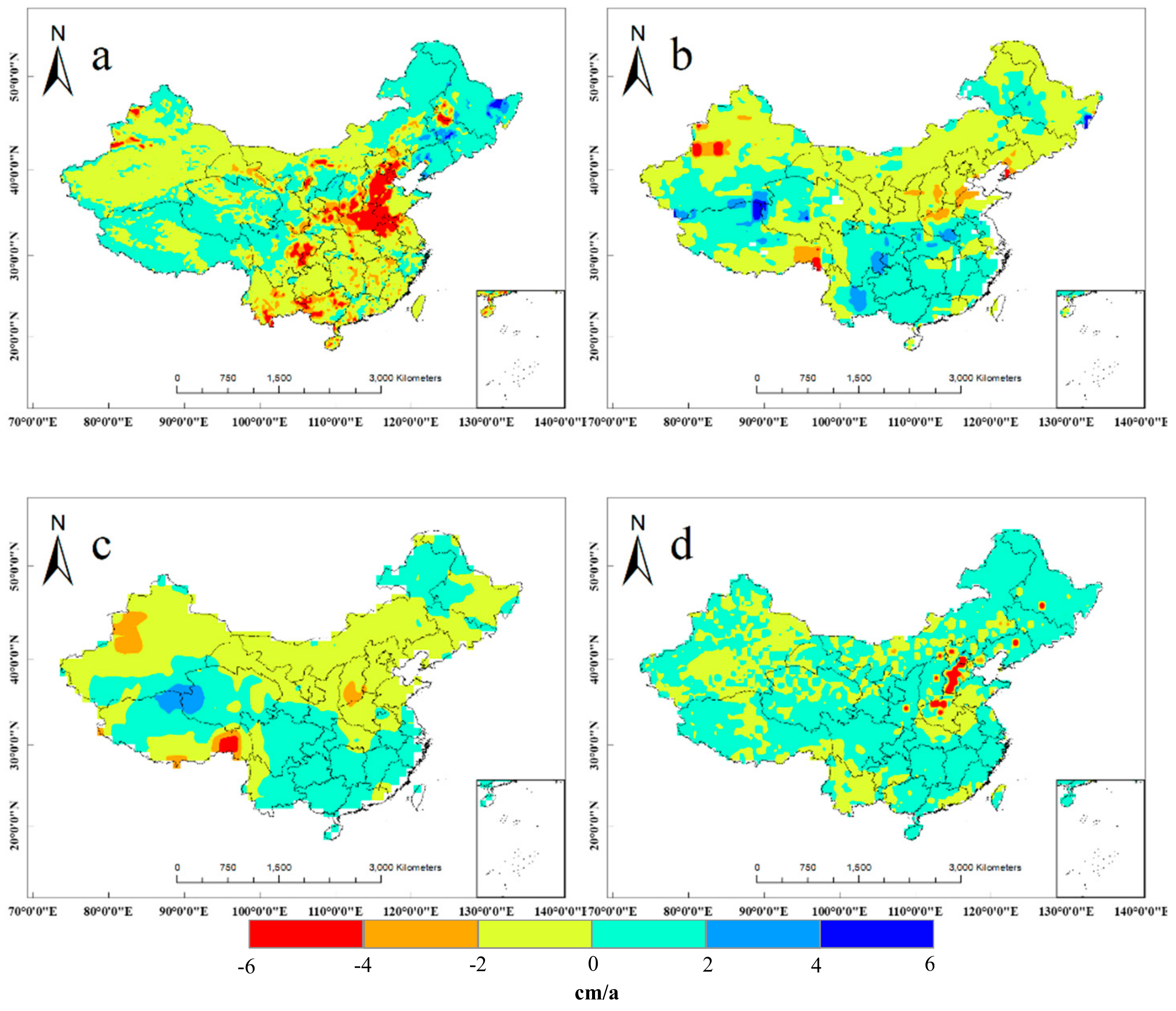
The Sen’s slopes of the derived GWS from the different datasets from 2005 to 2013 were calculated for China (Figure 1). The time period from 2005 to 2013 was selected because the observation wells data were only available for this time period. Since there are 30 combinations of derived GWS from GRACE combined with GLDAS and E2O, here, we only present the two best results, i.e., JPLMS combined with GLDAS Noah V2.1 and JPLMS combined with E2O according to the comparison with the in situ measurements that follow. The results of the complete datasets can be referred to Figure S1 in the Supplementary file. The results show that the annual trends of GWS derived from GRACE JPLMS combined with E2O (Figure 1b) and GRACE JPLMS combined with GLDAS Noah V2.1 (Figure 1c) shows similar spatial patterns—an increasing trend in southern China and a significant decrease in the NCP. GWS derived from E2O (Figure 1a) shows quite different patterns where a particularly clear increase in GWS in northeastern China and a decline in Tibet Plateau were observed, while the GWS derived from WGHM (Figure 1d) shows increasing trends in most parts of China and a severe decline in the NCP.

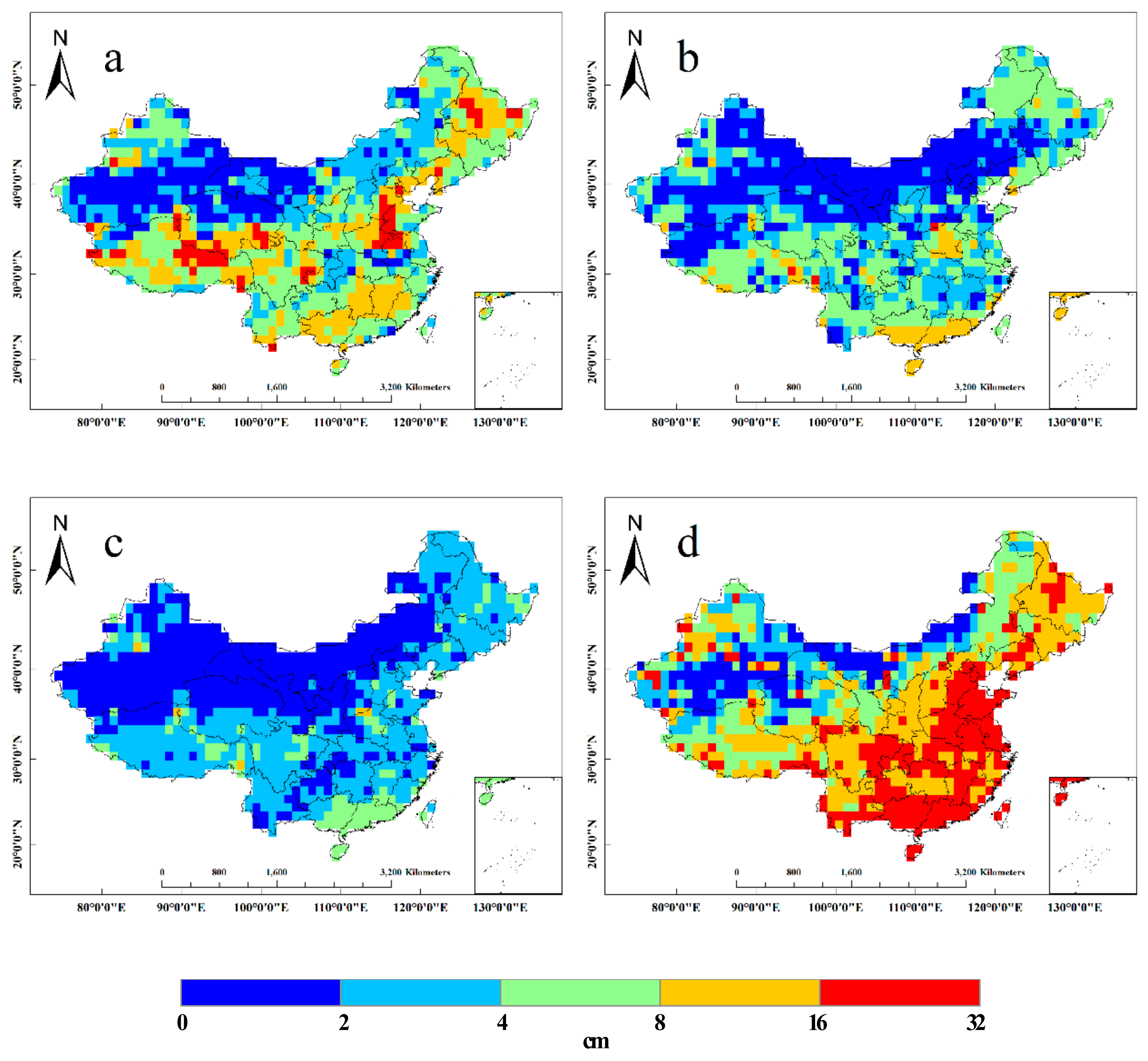
Figure 2 gives the uncertainties of the GWS derived from different datasets computed from the TCH method given in Section 2.2.4. We can see that the GWS derived from GRACE JPLMS combined with E2O (Figure 2b) and GWS derived from GRACE JPLMS combined with GLADAS Noah V2.1 (Figure 2c) have relatively low uncertainties, with national average uncertainties of 3.7 cm and 2.28 cm, respectively. The GWS derived from WGHM exhibits the largest uncertainties with a national average uncertainty of 13.1 cm, and the largest uncertainties were observed in southern China and the NCP.

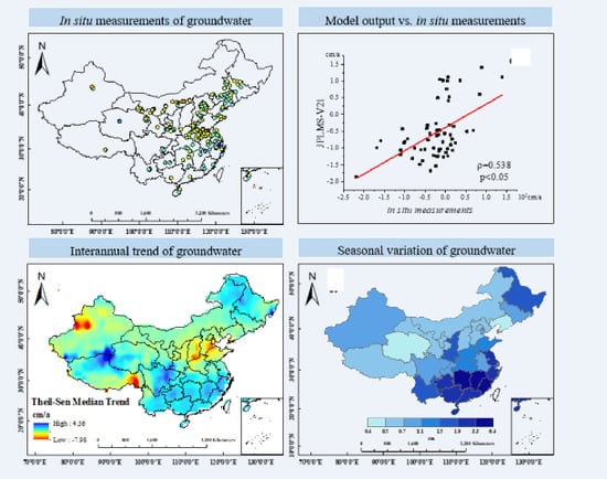
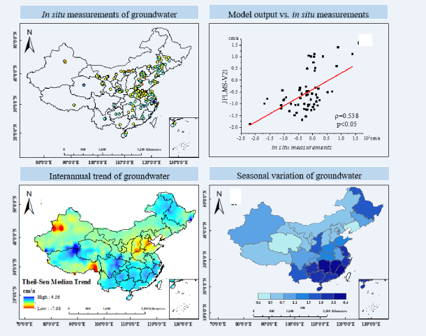
We further compared the changes in GWS from the four approaches presented above with changes in groundwater levels change from observation wells. Figure 3 presents the spatial temporal trend of GWS based on recorded data from observation wells with statistical significance at the 5% level under the conditions of the MK test (p <0.05). In general, there is an increasing trend in GWS in southern China and a decreasing trend in northern China.

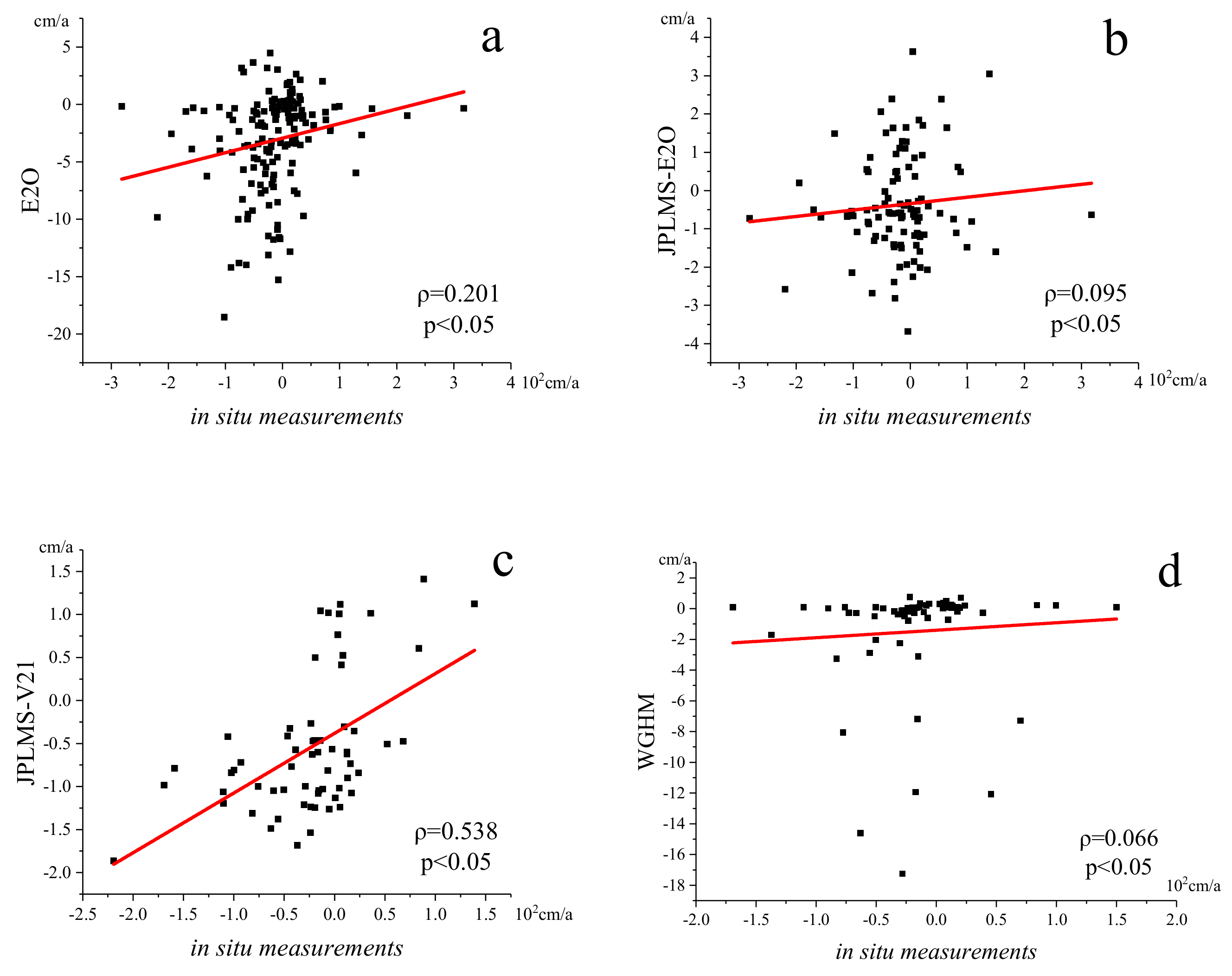
Figure 4 shows that the correlation coefficients between the annual trend derived from in situ measurements and GRACE JPLMS combined with hydraulic models, and the annual trends of observation wells in the same grid were averaged. Two limitations of this comparison have to be addressed, i.e., (1) there is a spatial mismatch between the global resolution data and point scale measurements; (2) the in situ measurements measure the groundwater level change instead of ground water storage change. Nevertheless, this comparison measures how strong a relationship is between the two from a general perspective. From Figure 3, we can see that the derived GWS range from 0.066 to 0.538 (p < 0.05). The GWS derived from GRACE JPLMS and GLDAS Noah V2.1 have the best correlation with the observed data, while the GWS derived from WGHM have the worst correlation. The results imply that the GRACE JPL Mascons products combined with the GLDAS Noah V2.1 data was a relatively reasonable and reliable dataset to represent GWS changes in China. This dataset was therefore adopted for further analysis and the time period of the GWS data was extended from 2005–2013 to 2003–2016.

3.2. EOF Analysis of GWS Changes in China

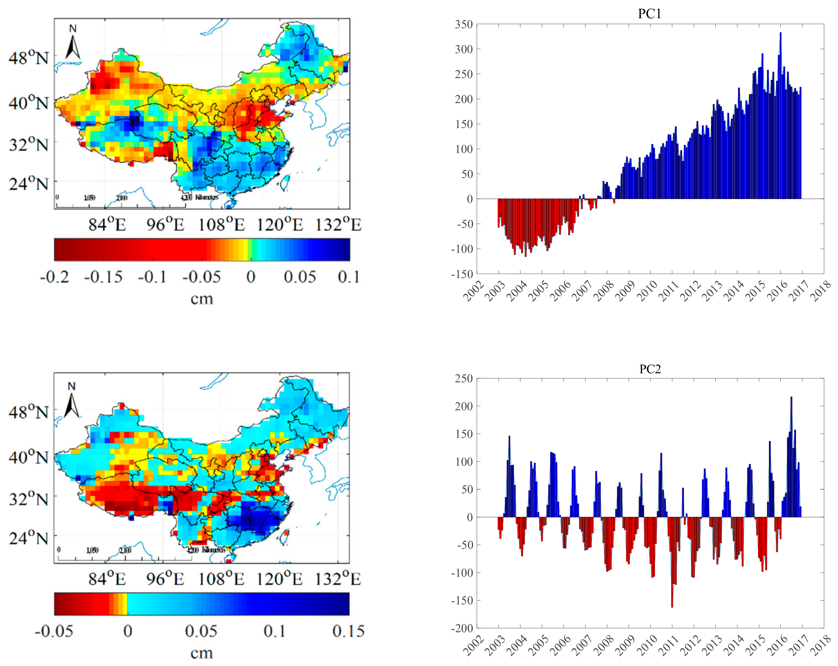
We decomposed the monthly GWS time series from 2003 to 2016 using the EOF method. Figure 5 shows the spatial patterns (EOF model 1 and mode 2) of the GWS changes and the associated principle components (PC1 and PC2). The long-term trends and seasonal variability were captured by the first two modes of the EOF analysis, which explain 52.61% and 13.19% of the total variance, respectively.

PC1 is associated with the long-term trends and interannual variability of GWS. A climatological shift occurred in August between 2007 and 2008. The spatial pattern of mode 1 shows positive GWS deviations in southeast China, the Qinghai-Tibet Plateau, and the Heilongjiang River Basin but negative deviations in most part of North China, especially Tien Shan region in northwestern China’s Xinjiang Province, southern Tibet, and the NCP. Combined with amplitude time series PC1, the results show that the GWS changes in southeast China, the Qinghai-Tibet Plateau, and the Heilongjiang River Basin decreased during 2003–2007 and increased during 2008–2016, while other regions had the opposite pattern, indicating that they experienced GWS decrease after 2008.

PC2 is associated with the dominant seasonal features. The amplitude of PC2 approximates a sine wave with peaks in May - September and troughs in December - March. Combined with the spatial pattern of mode 2, we can see an increasing trend for the GWS change between May and September and a decreasing trend between December and March in southeast China, northeastern China (Heilongjiang, Jilin, and Liaoning provinces and the Inner Mongolia Autonomous Region), and the northwestern part of Xinjiang.

It is known that precipitation plays an important role in replenishing the GWS. In the next section, we quantify how GWS is influenced by precipitation variability throughout China.

3.3. Interannual Variation in GWS

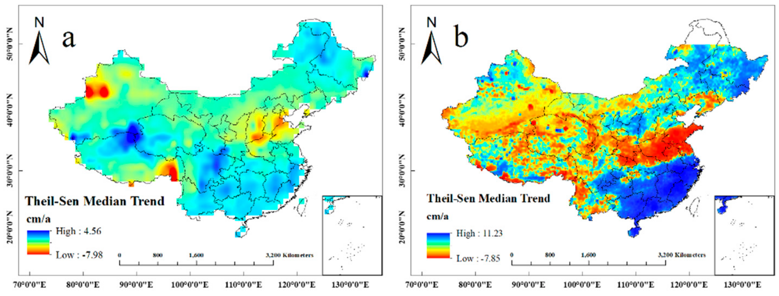
The interannual trends of GWS during 2003-2016 were calculated and are shown in Figure 6a. The results show clear regional characteristics of GWS changes. In southern China, including Sichuan, Chongqing, Hubei, Anhui, and Jiangsu provinces, there were clear increasing trends. Increasing trends were also observed in most of the Qinghai-Tibet region (except the southeast corner), the northeastern Inner Mongolia Autonomous Region and Heilongjiang Province. Significant declines in GWS were observed in the Tien Shan region in northwest of China’s Xinjiang Province, southeastern Tibet, and the NCP. The largest decrease was –7.98 cm/a in southeastern Tibet.

We analyzed the correlation between precipitation and GWS at the provincial level. Figure 6 shows the trends of annual precipitation and GWS in China during 2003–2016. The results show significant increases in precipitation in southeastern and northeastern China, which correspond to increases in GWS in the corresponding regions, while most regions of Northern China show decreasing trends in precipitation which is also highly consistent with the decreasing trend of GWS. However, inconsistency exists between the two. For example, an apparent GWS decrease was found in the east of Himalaya Mountains, northern Tarim Basin but not for the precipitation. Due to the fact that the glacier mass change was not excluded from GRACE [56], the decrease was mainly caused by glacier mass change rather than GWS depletion [57,58,59,60,61]. The GWS showed a clear increase in Qinghai-Tibet while there was a decrease in precipitation. Although the precipitation in this region shows a declining trend from 2003 to 2016, the average precipitation was 242.99 mm yr⁻¹, larger than the 1998–2002 average of 224.31 mm yr⁻¹. The increasing trend of GWS is mainly due to the replenishment of GWS after a prolonged dry period from 1998–2002 [61]. We also found that despite increases in precipitation in Beijing, Tianjin, Hebei, and Shanxi, which are partially or wholly in the NCP, there was a severe decrease in GWS.

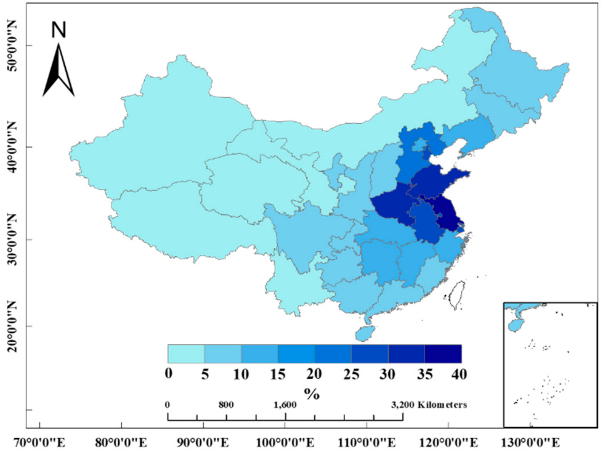
We further calculated the correlation coefficients between the trend of GWS and precipitation at the provincial level (Figure 7). There is a relatively high correlation of 0.573 between the interannual variations in the TRMM data and the GWS. The correlation between the two would reach 0.73 when four provinces (Beijing, Tianjin, Hebei, and Shanxi) which are mainly in or around the NCP were excluded. It is well known that the groundwater depletion is seriously affected by the anthropogenic factors in the NCP [1,26,61]. Figure 8 shows the ratio of average irrigated area of cultivated land at provincial level from 2003-2016 and the GWS consumption was the largest in the NCP and the pattern was highly consistent with GWS depletion depicted in Figure 5a. The NCP is the premier irrigated area in China and the Plain has 17,950 thousand ha of cultivated land, about 71.7 percent of which is irrigated and the crop production largely relies on underground water [62,63]. The increase of coefficient between GWS and TRMM when four provinces (Beijing, Tianjin, Hebei, and Shanxi) were excluded also proves the influence of human factors in the NCP.

3.4. Seasonal Variation in GWS

In addition to the interannual variation, we also investigated the GWS fluctuations during the year. Fluctuations in GWS may lead to ground settlement, which can pose great risks to infrastructure [2].

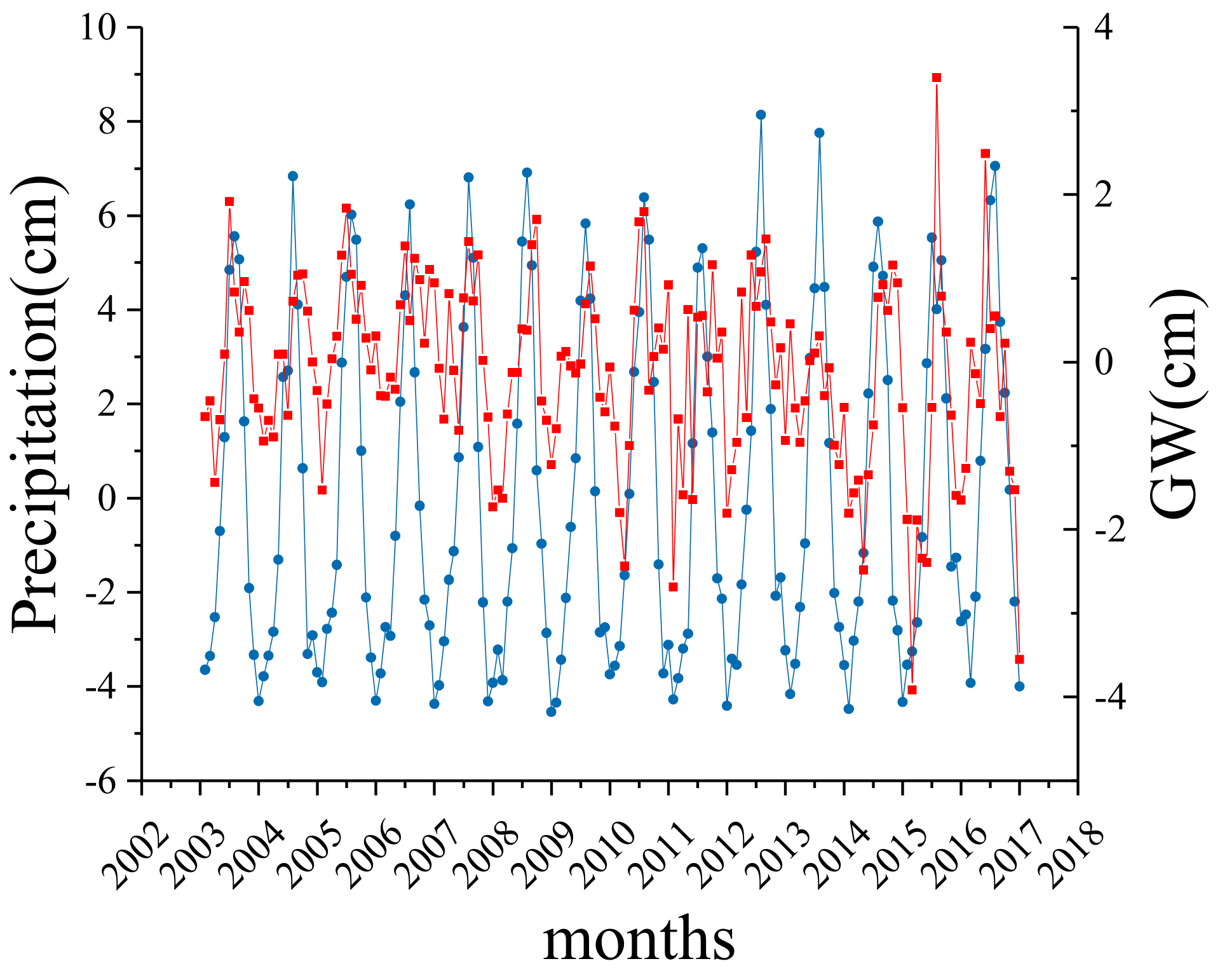
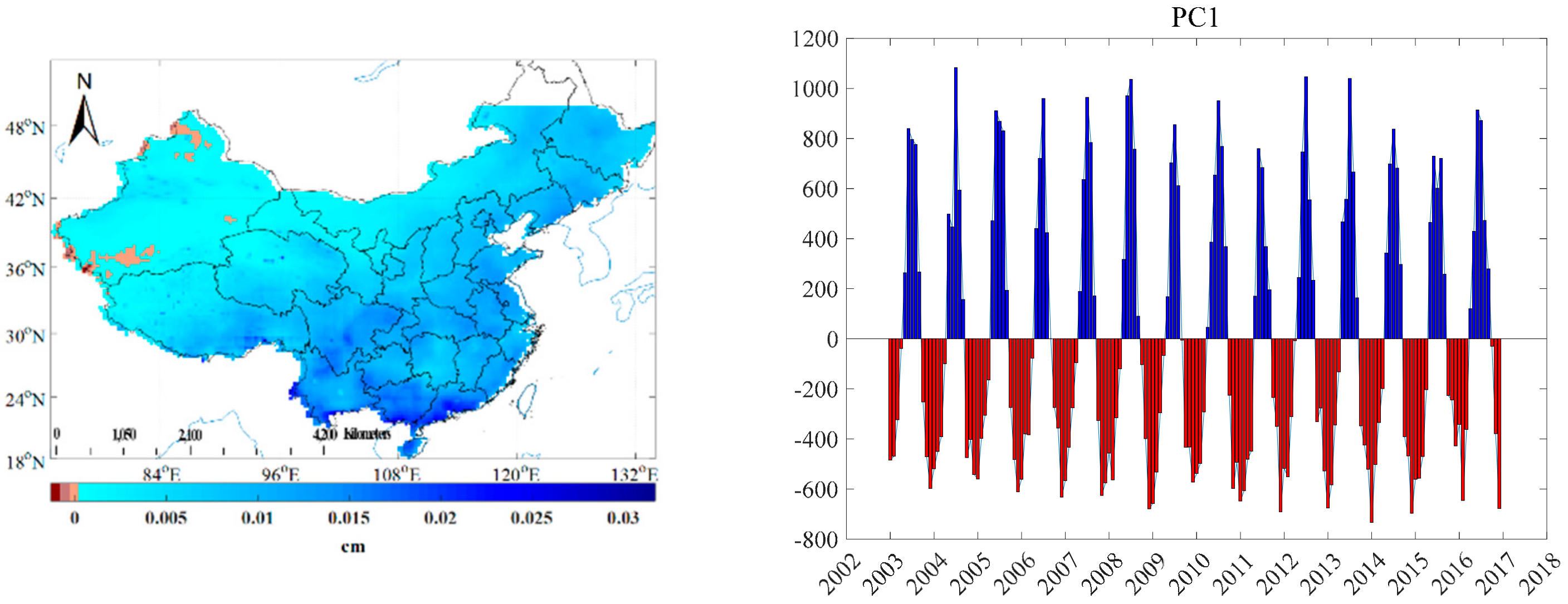
Figure 9 shows the fluctuations in the time series of GWS and precipitation from 2003 to 2016. The peaks and troughs are highly consistent, and the correlation coefficient is 0.52. These results show that GWS changes are substantially affected by rainfall throughout China. We then decomposed precipitation from the TRMM data using the EOF method to determine the seasonal variation. Detrend of the anomalies derived from precipitation was performed. As shown in Figure 10, the amplitude of PC1, which explains 53.59% of the total precipitation variability, shows similar seasonal cycles as GWS. Troughs exist from January to April and from October to December, and peaks are observed from May to September. This indicates that the amplitude time series of mode 1 captures the 5-month phase shift of the monsoon season (May - September). A comparison of PC2 of GWS and PC1 of precipitation shows that the seasonal variation in GWS is highly consistent with the seasonal variation in precipitation, indicating that precipitation plays an important role in GWS changes. The correlation coefficient is 0.76 and this indicates that the seasonal change in precipitation can be a reliable indicator of the seasonal change in GWS.

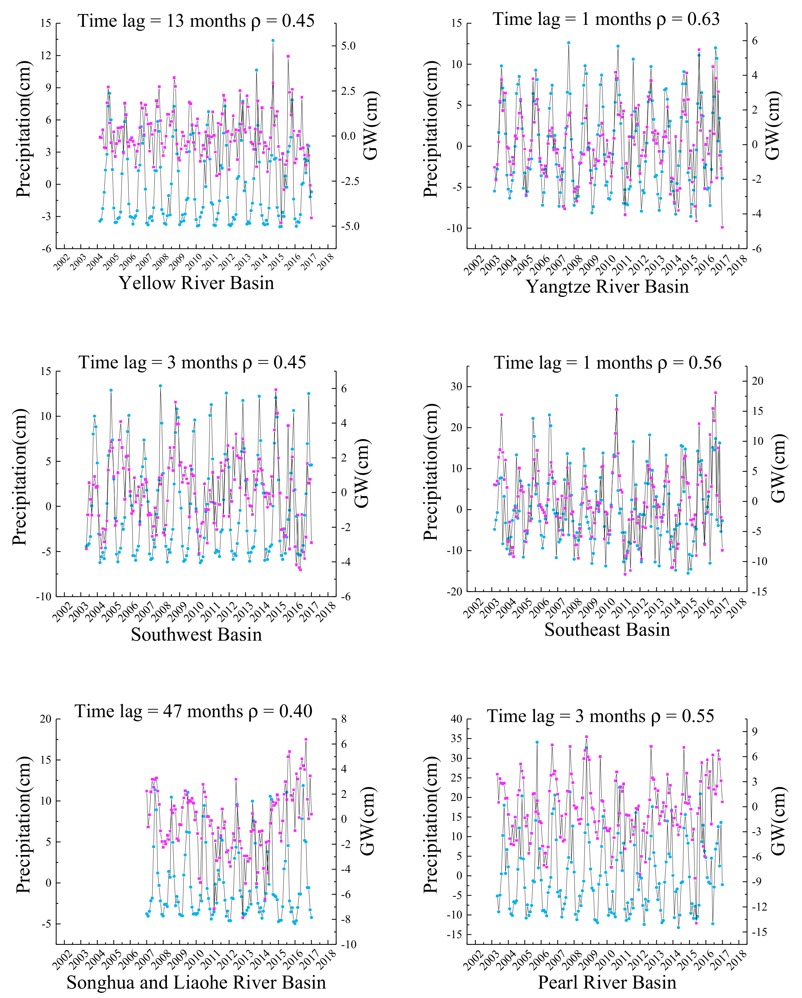
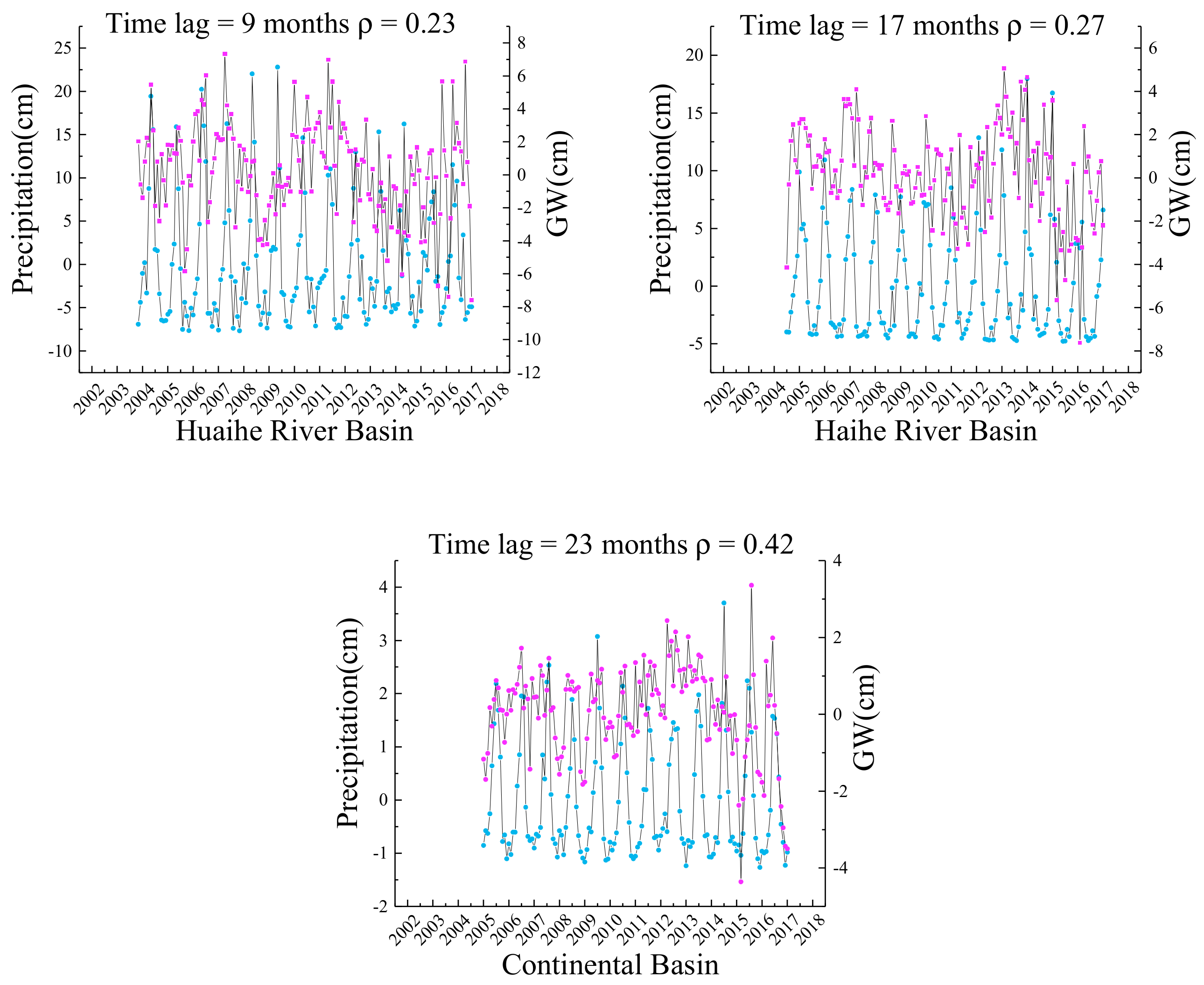
To further investigate the relationship between precipitation and GWS, we computed the seasonal fluctuation of main river basins [64]: Songhua and Liaohe River Basin (SLRB), Continental Basin (CB), Haihe River Basin (HRB), Huaihe River Basin (HHRB), Southwest Basin (SWB), Southeast Basin (SEB), Yangtze River Basin (YZRB), Pearl River Basin (PRB), Yellow River Basin (YRB) (Figure 11). Figure 12 shows the calculated correlation coefficients between the GWS and precipitation for 9 river basins at a maximum time lag of 48 months. We can see that correlations are significant (ρ > 0.4) in 7 of the 9 river basins. The maximum correlation (ρ = 0.63) was observed in Yangtze River Basin with a time lag of 1 month. Haihe River Basin (ρ = 0.27 at 17 months) and Huaihe River Basin (ρ = 0.23 at 9 months) showed the lowest correlations and responded at long time scales. These two basins are located in the NCP and the results highlight the effect of human activities on the GWS response to precipitation.

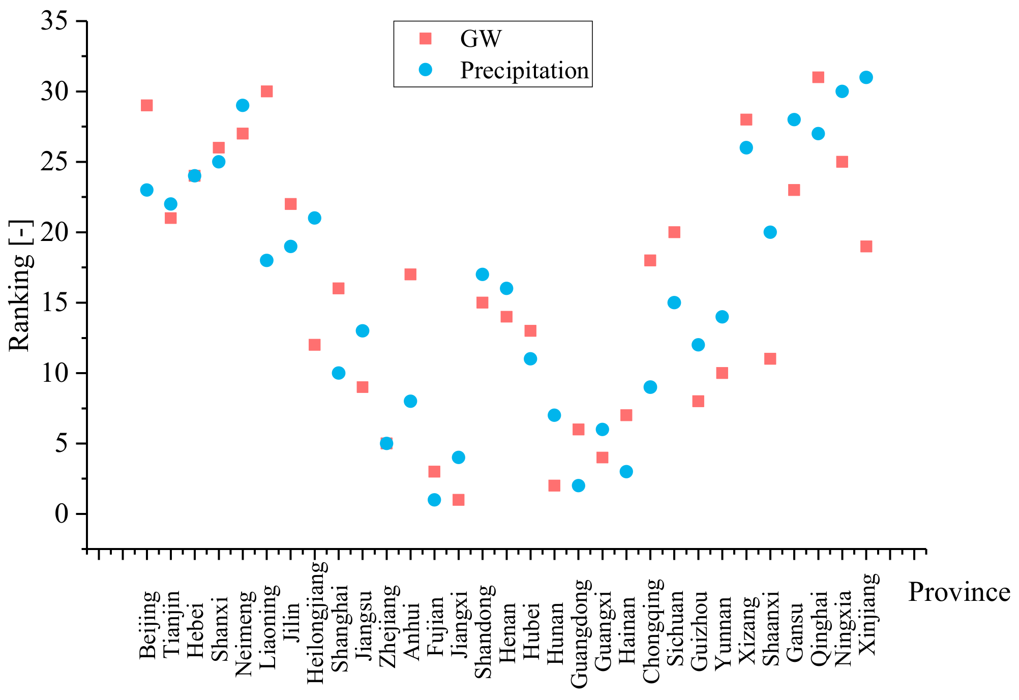
The fluctuation in GWS at the provincial level was quantified. We calculated the standard deviation of annual GWS derived from monthly climatological means in GWS change based on data from 2003-2016. The results show that the greatest fluctuation of GWS is in Jiangxi province and the standard deviation is 6.39 cm. Hunan and Fujian provinces also have large fluctuations of 6.33 cm and 5.20 cm, respectively. Generally, the fluctuation in GWS is fairly consistent with the annual precipitation (Figure 13): higher fluctuations of GWS occur in areas with higher annual precipitation, except for Xinjiang Province, where a relatively large fluctuation of GWS and low annual precipitation are observed. To quantify the correlation between precipitation and GWS fluctuation, we compared the ranking of provinces by seasonal fluctuations of GWS change and annual precipitation. The result is shown in Figure 14. It can be seen that there is a high consistency between the two and the correlation reaches 0.74. The top seven provinces with the highest groundwater fluctuations are exactly the same as the top seven provinces with the highest annual precipitation, which are Jiangxi, Hunan, Fujian, Guangxi, Zhejiang, Guangdong, and Hainan.

4. Conclusions

We compared GWS values derived from different combinations of GRACE and hydrological models data with in situ measurements at a national scale of China for the first time. The results indicate that GWS derived from JPLMS combined with GLDAS Noah V2.1 outperforms to reflect the spatiotemporal variations throughout China shown by the in situ observations, which provides guidance for choosing an appropriate method to derive the GWS of China.

A comprehensive analysis of GWS change in China was analyzed, including spatial patterns, interannual changes, seasonal fluctuations, etc. China’s GWS changes show clear interannual trends and seasonal variations during the period of 2003-2016. The change rate of regional GWS in China varied spatially, which was mainly reflected in generally increasing trends in the south-central region, the junction between Heilongjiang and Inner Mongolia and Xinjiang-Qinghai-Tibet boundaries. Significant declines in GWS were observed in the Tien Shan region in northwest of China’s Xinjiang Province, southern Tibet, and the NCP. The largest decrease was −7.98 cm/a in the southeastern Tibet. The interannual trends of GWS in most regions were consistent with those of precipitation but not in part of the NCP. Social and human factors could be significant drivers of the decreasing trend of GWS in the NCP.

The seasonal fluctuations of GWS in China were consistent with the precipitation. China’s precipitation showed peaks during May–September, and the peaks period of precipitation override the peaks of GWS. A low correlation was observed for Haihe River Basin (ρ = 0.27 at 17 months) and Huaihe River Basin (ρ = 0.23 at 9 months) which are located in the NCP, which also highlights the effect of human activities on the GWS response to precipitation. Provinces with large GWS fluctuations are identified. The awareness of areas with significant depletion and large seasonal variation of GWS help adaptations to cope with local GWS situation.

We have to admit that the method used in this study to derive GWS is imperfect and uncertainties exist. Recently, data assimilation techniques have been proposed to improve the simulation of hydrological models by assimilating the GRACE observation into hydraulic models [65,66,67,68,69]. We will use these new techniques in our future studies to enhance the accuracy of the GWS estimate. Meanwhile, further studies will be performed to quantify the contribution of natural and human-induced processes on the GWS of China at a provincial scale and hydrological settings.

References

- Aeschbach-Hertig, W.; Gleeson, T. Regional strategies for the accelerating global problem of groundwater depletion. Nat. Geosci. 2012, 5, 853–861. [Google Scholar] [CrossRef]
- Kang, G. Influence and Control Strategy for Local Settlement for High-Speed Railway Infrastructure. Engineering 2016, 2, 374–379. [Google Scholar] [CrossRef] [Green Version]
- Liu, J.; Yao, H.-l.; Hu, M.-l.; Lu, Z.; Yu, D.-m.; Chen, F.-g. Study of moisture dynamic response and underground drainage test of subgrade model under water level fluctuation. Rock Soil Mech. 2012, 33, 2917–2922. [Google Scholar]
- Wu, B. Three-dimensional seepage-stress coupling analysis of bridge foundation behaviors induced by precipitation. Chin. J. Rock Mech. Eng. 2009, 28, 3277–3281. [Google Scholar]
- Xia, L.-n.; Miao, Y.-d.; LIAO, C.-b. Three-dimensional numerical simulation of influences of ground subsidence on composite foundation. Rock Soil Mech. 2012, 33, 1217–1222. [Google Scholar]
- Feng, W.; Shum, C.; Zhong, M.; Pan, Y. Groundwater storage changes in China from satellite gravity: An overview. Remote Sens. 2018, 10, 674. [Google Scholar] [CrossRef] [Green Version]
- Rodell, M.; Houser, P.; Jambor, U.; Gottschalck, J.; Mitchell, K.; Meng, C.-J.; Arsenault, K.; Cosgrove, B.; Radakovich, J.; Bosilovich, M. The global land data assimilation system. Bull. Am. Meteorol. Soc. 2004, 85, 381–394. [Google Scholar] [CrossRef] [Green Version]
- Chen, F.; Mitchell, K.; Schaake, J.; Xue, Y.; Pan, H.L.; Koren, V.; Duan, Q.Y.; Ek, M.; Betts, A. Modeling of land surface evaporation by four schemes and comparison with FIFE observations. J. Geophys. Res. Atmos. 1996, 101, 7251–7268. [Google Scholar] [CrossRef] [Green Version]
- Koster, R.D.; Suarez, M.J. Modeling the land surface boundary in climate models as a composite of independent vegetation stands. J. Geophys. Res. Atmos. 1992, 97, 2697–2715. [Google Scholar] [CrossRef]
- Liang, X.; Lettenmaier, D.P.; Wood, E.F.; Burges, S.J. A simple hydrologically based model of land surface water and energy fluxes for general circulation models. J. Geophys. Res. Atmos. 1994, 99, 14415–14428. [Google Scholar] [CrossRef]
- Lawrence, D.M.; Oleson, K.W.; Flanner, M.G.; Thornton, P.E.; Swenson, S.C.; Lawrence, P.J.; Zeng, X.; Yang, Z.-L.; Levis, S.; Sakaguchi, K.; et al. Parameterization improvements and functional and structural advances in Version 4 of the Community Land Model. J. Adv. Model. Earth Syst. 2011, 3. [Google Scholar] [CrossRef]
- Clark, D.B.; Mercado, L.M.; Sitch, S.; Jones, C.D.; Gedney, N.; Best, M.J.; Pryor, M.; Rooney, G.G.; Essery, R.L.H.; Blyth, E.; et al. The Joint UK Land Environment Simulator (JULES), model description—Part 2: Carbon fluxes and vegetation dynamics. Geosci. Model Dev. 2011, 4, 701–722. [Google Scholar] [CrossRef] [Green Version]
- Alcamo, J.; Döll, P.; Kaspar, F.; Siebert, S. Global Change and Global Scenarios of Water Use and Availability: An Application of WaterGAP 1.0; Center for Environmental Systems Research: Kassel, Germany, 1997. [Google Scholar]
- Vörösmarty, C.J.; Federer, C.A.; Schloss, A.L. Potential evaporation functions compared on US watersheds: Possible implications for global-scale water balance and terrestrial ecosystem modeling. J. Hydrol. 1998, 207, 147–169. [Google Scholar] [CrossRef]
- Van Beek, L.P.H.; Bierkens, M.F.P. The Global Hydrological Model PCR-GLOBWB: Conceptualization, Parameterization and Verification; Report Department of Physical Geography, Utrecht University : Utrecht, The Netherlands, 2009; Available online: http://vanbeek.geo.uu.nl/suppinfo/vanbeekbierkens2009.pdf.
- Bierkens, M.F.P. Global hydrology 2015: State, trends, and directions. Water Resour. Res. 2015, 51, 4923–4947. [Google Scholar] [CrossRef]
- Döll, P.; Müller Schmied, H.; Schuh, C.; Portmann, F.T.; Eicker, A. Global-scale assessment of groundwater depletion and related groundwater abstractions: Combining hydrological modeling with information from well observations and GRACE satellites. Water Resour. Res. 2014, 50, 5698–5720. [Google Scholar] [CrossRef]
- Rodell, M.; Velicogna, I.; Famiglietti, J.S. Satellite-based estimates of groundwater depletion in India. Nature 2009, 460, 999. [Google Scholar] [CrossRef] [Green Version]
- Güntner, A. Improvement of global hydrological models using GRACE data. Surv. Geophys. 2008, 29, 375–397. [Google Scholar] [CrossRef] [Green Version]
- Landerer, F.W.; Swenson, S. Accuracy of scaled GRACE terrestrial water storage estimates. Water Resour. Res. 2012, 48, 4531. [Google Scholar] [CrossRef]
- Swenson, S.; Wahr, J. Post-processing removal of correlated errors in GRACE data. Geophys. Res. Lett. 2006, 33. [Google Scholar] [CrossRef]
- Watkins, M.M.; Wiese, D.N.; Yuan, D.-N.; Boening, C.; Landerer, F.W. Improved methods for observing Earth’s time variable mass distribution with GRACE using spherical cap mascons. J. Geophys. Res. Solid Earth 2015, 120, 2648–2671. [Google Scholar] [CrossRef]
- Wiese, D.N.; Landerer, F.W.; Watkins, M.M. Quantifying and reducing leakage errors in the JPL RL05M GRACE mascon solution. Water Resour. Res. 2016, 52, 7490–7502. [Google Scholar] [CrossRef]
- Save, H.; Bettadpur, S.; Tapley, B.D. High-resolution CSR GRACE RL05 mascons. J. Geophys. Res. Solid Earth 2016, 121, 7547–7569. [Google Scholar] [CrossRef]
- Huang, Z.; Pan, Y.; Gong, H.; Yeh, P.J.F.; Li, X.; Zhou, D.; Zhao, W. Subregional-scale groundwater depletion detected by GRACE for both shallow and deep aquifers in North China Plain. Geophys. Res. Lett. 2015, 42, 1791–1799. [Google Scholar] [CrossRef]
- Feng, W.; Zhong, M.; Lemoine, J.M.; Biancale, R.; Hsu, H.T.; Xia, J. Evaluation of groundwater depletion in North China using the Gravity Recovery and Climate Experiment (GRACE) data and ground-based measurements. Water Resour. Res. 2013, 49, 2110–2118. [Google Scholar] [CrossRef]
- Wang, X.; de Linage, C.; Famiglietti, J.; Zender, C.S. Gravity Recovery and Climate Experiment (GRACE) detection of water storage changes in the Three Gorges Reservoir of China and comparison with in situ measurements. Water Resour. Res. 2011, 47. [Google Scholar] [CrossRef]
- Zhong, Y.; Zhong, M.; Feng, W.; Zhang, Z.; Shen, Y.; Wu, D. Groundwater depletion in the West Liaohe River Basin, China and its Implications revealed by GRACE and in situ measurements. Remote Sens. 2018, 10, 493. [Google Scholar] [CrossRef] [Green Version]
- Shen, H.; Leblanc, M.; Tweed, S.; Liu, W. Groundwater depletion in the Hai River Basin, China, from in situ and GRACE observations. Hydrol. Sci. J. 2015, 60, 671–687. [Google Scholar] [CrossRef] [Green Version]
- Shamsudduha, M.; Taylor, R.; Longuevergne, L. Monitoring groundwater storage changes in the highly seasonal humid tropics: Validation of GRACE measurements in the Bengal Basin. Water Resour. Res. 2012, 48. [Google Scholar] [CrossRef] [Green Version]