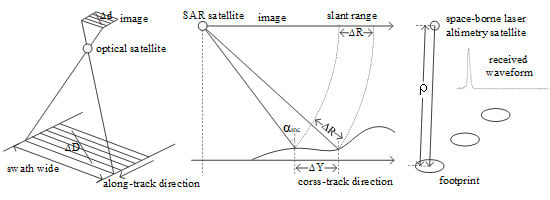
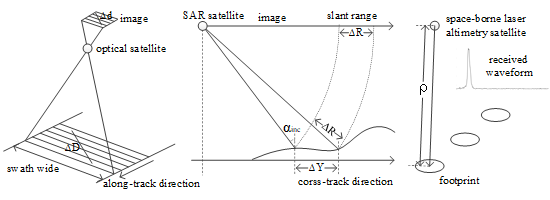
Article

Geometric Accuracy Improvement Method for High-Resolution Optical Satellite Remote Sensing Imagery Combining Multi-Temporal SAR Imagery and GLAS Data

1
The State Key Laboratory of Information Engineering in Surveying, Mapping, and Remote Sensing, Wuhan University, Wuhan 430079, China
2
Institute of Applied Environmental Health, School of Public Health, University of Maryland, College Park, MD 20742, USA
*
Author to whom correspondence should be addressed.
Remote Sens. 2020, 12(3), 568; https://doi.org/10.3390/rs12030568
Submission received: 30 December 2019 / Revised: 4 February 2020 / Accepted: 6 February 2020 / Published: 8 February 2020

Abstract

:
With the widespread availability of satellite data, a single region can be described using multi-source and multi-temporal remote sensing data, such as high-resolution (HR) optical imagery, synthetic aperture radar (SAR) imagery, and space-borne laser altimetry data. These have become the main source of data for geopositioning. However, due to the limitation of the direct geometric accuracy of HR optical imagery and the effect of the small intersection angle of HR optical imagery in stereo pair orientation, the geometric accuracy of HR optical imagery cannot meet the requirements for geopositioning without ground control points (GCPs), especially in uninhabited areas, such as forests, plateaus, or deserts. Without satellite attitude error, SAR usually provides higher geometric accuracy than optical satellites. Space-borne laser altimetry technology can collect global laser footprints with high altitude accuracy. Therefore, this paper presents a geometric accuracy improvement method for HR optical satellite remote sensing imagery combining multi-temporal SAR Imagery and GLAS data without GCPs. Based on the imaging mechanism, the differences in the weight matrix determination of the HR optical imagery and SAR imagery were analyzed. The laser altimetry data with high altitude accuracy were selected and applied as height control point in combined geopositioning. To validate the combined geopositioning approach, GaoFen2 (GF2) optical imagery, GaoFen6 (GF6) optical imagery, GaoFen3 (GF3) SAR imagery, and the Geoscience Laser Altimeter System (GLAS) footprint were tested. The experimental results show that the proposed model can be effectively applied to combined geopositioning to improve the geometric accuracy of HR optical imagery. Moreover, we found that the distribution and weight matrix determination of SAR images and the distribution of GLAS footprints are the crucial factors influencing geometric accuracy. Combined geopositioning using multi-source remote sensing data can achieve a plane accuracy of 1.587 m and an altitude accuracy of 1.985 m, which is similar to the geometric accuracy of geopositioning of GF2 with GCPs.

Graphical Abstract

1. Introduction

High-resolution (HR) optical satellite imagery has become an important data source for geopositioning due to the wide coverage, short return period, and good image interpretation [1]. Due to the limitation of the direct geometric accuracy of HR optical imagery, some ground control points (GCPs) are usually adopted to compensate for geometric errors in HR optical imagery to meet the geometric accuracy requirements of geopositioning [2,3,4,5,6]. However, the lack of access to some uninhabited areas, such as forests, plateaus, or deserts, prevents the acquisition of GCPs, so the plane accuracy cannot meet the requirements for geopositioning. HR optical satellite images are usually acquired with nadir or near-nadir imaging geometry. Therefore, affected by the small intersection angle of HR optical imagery in stereo pair orientation, the altitude accuracy also cannot meet the geopositioning requirements.
Given the widespread availability of satellite data, a single region can be described by multi-source and multi-temporal remote sensing data, such as SAR imagery and laser altimetry data. Without satellite attitude error, SAR usually provides higher geometric accuracy than optical satellites [7]. However, SAR satellite imagery has more noise than HR optical imagery [8]. SAR satellite images usually have a small coverage area and cannot meet the needs of large-area geopositioning. Space-borne laser altimetry technology can collect global laser footprints with high altitude accuracy [9]. However, the laser footprints of current space-borne laser altimetry technology are more discrete and cannot express the detailed information of the ground surface. Therefore, combined geopositioning using multi-source and multi-temporal remote sensing data could be applied to improve the geometric accuracy of optical imagery without GCPs.
Several studies have focused on geometric accuracy improvement methods for HR optical satellite remote sensing imagery using multi-source and multi-temporal remote sensing data. Jeong and Kim studied the geometric accuracy and imaging geometry of dual-sensor stereo pairs in comparison with those of conventional single-sensor stereo pairs. Then, they investigated the influences of convergence angle, bisector elevation angle, and asymmetry angle on geometric accuracy for dual-sensor stereo pair orientation [10]. Jeong et al. investigated the positioning accuracy of multiple-satellite images. Using IKONOS, QuickBird, and KOMPSAT-2 data for Daejeon, Korea, they revealed the potential, limitations, and important considerations for geopositioning applications using images from multiple satellites [11]. Based on the rigorous combined geopositioning model for optical and SAR imagery, Xing et al. discussed the construction of an observation equation, computation of the weight matrix, and the frame of computation process, and further analyzed geometric accuracy with GCPs [12]. Zhang et al. validated the application of the universal rational function model (RFM) for optical and SAR stereo pair combined orientation [13]. Cheng et al. analyzed the influences of the number of SAR images, orbit direction of the SAR satellite, and the distribution of SAR images on geometric accuracy using the RFM model [14]. The first Earth observation laser altimetry satellite, Ice Cloud and Land Elevation Satellite (ICESat-1), carrying the GLAS, was launched in 2003 [15,16,17,18]. With the advantages of high altitude accuracy, global distribution, and a large number of collected footprints, GLAS footprints are widely used for height reference in the calibration and validation of digital elevation models (DEMs) [19]. Some researchers have employed the GLAS footprint as height control points in optical imagery block adjustment, which significantly improved altitude accuracy [20]. Li et al. added two GLAS height control points for every ZiYuan-3 image in the block area, and the vertical accuracy satisfied the requirements doe 1:50,000 scale mapping [21]. However, few studies have been dedicated to the study of geometric accuracy improvement of HR optical images combined with SAR images and space-borne laser altimetry footprints, which could play an important role in geopositioning without GCPs. Therefore, analyzing the key factors influencing the geometric accuracy of combined geopositioning using multi-source remote sensing data without GCPs is required, which is important for high accuracy geopositioning in uninhabited areas.
This paper presents a geometric accuracy improvement method of HR optical satellite remote sensing imagery combining multi-temporal SAR Imagery and GLAS data. Based on error analysis of HR optical and SAR images, we prove that the affine transformation model in image space can effectively compensate for the unmodelled errors in the combined geopositioning model. Considering the imaging mechanisms of HR optical and SAR satellites, the weight determination of the combined geopositioning model is proposed in this paper. Based on the characteristics of GLAS products, the footprints located in flat areas with high altitude accuracy were selected as height control points for HR optical imagery combined geopositioning. Then, the observation equation was constructed using the GLAS control points. In our experiments, GF2 HR optical images, GF6 HR optical images, GF3 SAR images, and the GLAS footprint covering Dongying area in China were tested. The corresponding digital orthophotograph model (DOM) and DEM were applied as reference data to evaluate plane accuracy and altitude accuracy, respectively. The experimental results showed that the proposed model can be adopted for combined multi-source and multi-temporal remote sensing data geopositioning to improve geometric accuracy of HR optical satellite remote sensing imagery without GCPs. The distribution and weight matrix settings for SAR images and the number of GLAS footprints were found to be the crucial factors influencing the geometric accuracy. For GF2, multi-source combined geopositioning achieved a plane accuracy of 1.587 m and an altitude accuracy of 1.985 m, which is similar to the geometric accuracy of geopositioning of GF2 with GCPs. The geometric accuracies for GF6 multi-source combined geopositioning were a plane accuracy of 2.908 m and an altitude accuracy of 7.669 m, which is similar to the geometric accuracy of geopositioning of GF6 with GCPs.
The remainder of the paper is organized as follows: Section 2 demonstrates the methodology used to improve the geometric accuracy of HR optical satellite remote sensing imagery with the combined geopositioning method. Section 3 describes the experimental area and data and presents the experimental results and discussion. Section 4 summarizes our work and presents the study conclusions and research perspectives.

2. Methodology

2.1. Rational Polynomial Coefficients Model for Combined Geopositioning

The RFM model, in the form of rational polynomial coefficients (RPCs), connects the object coordinate ( B , L , H ) with the image coordinate ( l , s ) [22,23,24,25,26,27,28]. B , L , and H are the longitude, latitude, and ellipsoid height, respectively; l and s are the line and sample coordinates, respectively. This can be expressed by the following equation:
l n = N u m l ( U , V , W ) D e n l ( U , V , W ) s n = N u m s ( U , V , W ) D e n s ( U , V , W )
N u m l ( U , V , W ) = a 1 + a 2 V + a 3 U + a 4 W + a 5 V U + a 6 V W + a 7 U W + a 8 V 2 + a 9 U 2 + a 10 W 2 + a 11 U V W + a 12 V 3 + a 13 V U 2 + a 14 V W 2 + a 15 V 2 U + a 16 U 3 + a 17 U W 2 + a 18 V 2 W + a 19 U 2 W + a 20 W 3 D e n l ( U , V , W ) = b 1 + b 2 V + b 3 U + b 4 W + b 5 V U + b 6 V W + b 7 U W + b 8 V 2 + b 9 U 2 + b 10 W 2 + b 11 U V W + b 12 V 3 + b 13 V U 2 + b 14 V W 2 + b 15 V 2 U + b 16 U 3 + b 17 U W 2 + b 18 V 2 W + b 19 U 2 W + b 20 W 3 N u m s ( U , V , W ) = c 1 + c 2 V + c 3 U + c 4 W + c 5 V U + c 6 V W + c 7 U W + c 8 V 2 + c 9 U 2 + c 10 W 2 + c 11 U V W + c 12 V 3 + c 13 V U 2 + c 14 V W 2 + c 15 V 2 U + c 16 U 3 + c 17 U W 2 + c 18 V 2 W + c 19 U 2 W + c 20 W 3 D e n s ( U , V , W ) = d 1 + d 2 V + d 3 U + d 4 W + d 5 V U + d 6 V W + d 7 U W + d 8 V 2 + d 9 U 2 + d 10 W 2 + d 11 U V W + d 12 V 3 + d 13 V U 2 + d 14 V W 2 + d 15 V 2 U + d 16 U 3 + d 17 U W 2 + d 18 V 2 W + d 19 U 2 W + d 20 W 3
where a i , b i , c i , d i ( i = 1 , 2 , , 20 ) are the rational polynomial coefficients, and the values of b 1 , d 1 are usually set to 1. ( l n , s n ) , ( U , V , W ) are the normalized coordinates of the image coordinate ( l , s ) and the object coordinate ( L a t , L o n , H e i g h t ) , respectively, which ensures the stability of calculation of the RFM model. According to the following equations, the image coordinate and the object coordinate are normalized between –1 and 1.
l n = l - L i n e O f f L i n e S c a l e s n = s - S a m p l e O f f S a m p l e S c a l e
where L i n e O f f and S a m p l e O f f are the translation value of the image coordinate. L i n e S c a l e and S a m p l e S c a l e are the scale value of the image coordinate.
U = L o n - L o n O f f L o n S c a l e V = L a t - L a t O f f L a t S c a l e W = H e i g h t - H e i O f f H e i S c a l e
where L o n O f f , L a t O f f , and H e i O f f are the translation value of the object coordinate. L o n S c a l e , L a t S c a l e , and H e i S c a l e are the scale value of the object coordinate.
With the advantage of sensor independence, the RPC model can be used for both HR optical imagery and SAR imagery. Therefore, the RPC model was adopted here for combined geopositioning.

2.2. Orientation Error

Some errors occur during satellite data acquisition and processing, such as sensor errors, platform ephemeris errors, attitude measurement errors, and so on, causing offset errors, scale errors, and rotation errors in remote sensing imagery, as listed in Table 1.
The error sources of optical satellite and SAR satellite cause offset errors and linear or scale errors along or across the track direction. Therefore, to achieve perfect space intersection, the affine transformation model in image space is applied to compensate for existing geometric errors. The RPC model for combined geopositioning is as follows:
l + a 0 + a 1 × l + a 2 × s = F l ( L a t , L o n , H e i g h t ) s + b 0 + b 1 × l + b 2 × s = F s ( L a t , L o n , H e i g h t )
where a 0 and b 0 compensate for the offset error and a 1 , a 2 , b 1 , and b 2 compensate for the scale and rotation error.
Without GCPs, a data defect exists in the combined geopositioning model, which results in equation divergence [29]. Therefore, a pseudo-observation equation of the image affine transformation parameters was employed here to achieve combined geopositioning without GCPs. The integrated model for combined geopositioning using multi-source remote sensing data can be represented in matrix form as:
V 1 = B G X G + B A X A - L 1 P 1 V 2 = I X A - L 2 P 2
B G = l L a t l L o n l H e i g h t s L a t s L o n s H e i g h t , X G = L a t L o n H e i g h t
B A = l a 0 l a 1 l a 2 l b 0 l b 1 l b 2 s a 0 s a 1 s a 2 s b 0 s b 1 s b 2 , X A = a 0 a 1 a 2 b 1 b 2 b 3
where the first observation equation is relevant to the tie point and the second observation equation is the pseudo-observation equation. X G and X A are the object coordinates of tie points and the affine transformation parameters of images, respectively; B G and B A are coefficient matrixes derived from the derivatives of X G and X A ; I is the unit coefficient matrix; L 1 and L 2 are observations in the observation equations; and P 1 and P 2 are the weight matrixes. The weight P 1 relating to the tie points is set to one pixel because the measurement accuracy of image coordinates is usually achieved at one pixel. The weight P 2 relating to the affine transformation parameters is set according to the physical meaning and priori error of each parameter, expressed as:
P a 0 = 1 σ a 0 2 P b 0 = 1 σ b 0 2 P a 1 = P b 1 = 1 σ 1 2 P a 2 = P b 2 = 1 σ 2 2
where σ a 0 and σ b 0 are the offset errors along the line direction (row direction) and sample direction (column direction), respectively; σ 1 and σ 2 are the scale and rotation errors along the line direction and sample direction, respectively.

2.3. Combined Geopositioning with SAR

The relationships between object distance and image distance are different between HR optical imagery and SAR imagery due to the discrepancy in the imaging mechanisms. HR optical imagery applies central projection, as shown in Figure 1a. Therefore, the relationship between the object distance D and image distance d can be represented as follows:
d = D R o p t
where R o p t is the spatial resolution of HR optical imagery.
However, SAR imagery applies slant range projection in the cross-track direction. The sample distance in SAR imagery reflects the slant range distance to the object, not the cross-track distance, as shown in Figure 1b. Therefore, the relationship between the cross-track distance Y and sample distance s in the image can be expressed as follows:
s = Y × s i n α i n c R S A R _ s a m p l e
where α i n c is the incident angle and R S A R _ s a m p l e is the resolution along the sample direction in SAR images.
Therefore, the weight determination for the offset error compensation parameters differs. Based on the a priori geometric accuracy, offset error along the line direction and sample direction for HR optical imagery and SAR imagery can be calculated as follows:
σ a 0 = σ X R o p t σ b 0 = σ Y R o p t o p t σ a 0 = σ X R S A R _ l i n e σ b 0 = σ Y × s i n α i n c R S A R _ s a m p l e S A R
where σ X and σ Y are the along-track and cross-track geometric accuracy, respectively, and are usually calculated by the priori geometric accuracy σ , i.e., σ X = σ Y = σ / 2 . R S A R _ l i n e is the resolution along the line direction in SAR images.
The weight determination for the scale and rotation error compensation parameters is similar for both HR optical imagery and SAR imagery. They are usually determined by the maximum pixels M resulting from the scale, rotation, and size of the image [14], as follows:
σ 1 = M H σ 2 = M W
where H and W are the height and width of imagery, respectively.

2.4. Combined Geopositioning with GLAS

In flat areas, the altitude accuracy of the GLAS footprint can be as high as 15 cm [30,31,32,33,34,35]. However, due to the impact of outliers, clouds, slope, and vegetation, the altitude accuracy of the GLAS footprint is significantly lower, and cannot meet the altitude accuracy needs of geopositioning with high accuracy [36,37]. Therefore, to acquire GLAS footprints with high altitude accuracy, an extraction criterion including multiple constraints was applied. The second version of ASTER GDEM (GDEM2), attribute characteristic in the GLA14 product and waveform characteristic in the GLA01 product were used to select footprints with the thresholds defined in Table 2. Using GDEM2, the footprints with mistaken height values can be discarded. The GLA01 product is an altimetry data product that contains the received waveforms information required to produce higher accuracy range and elevation products. The number of peaks and the width of the waveform can reflect the characteristics of the topography and features. Given the constraints of waveforms, the footprints located in flat areas can be extracted. The GLA14 product is the land products file that contains the parameters of observation conditions and processing quality of the footprint. With the constraints of GLA14, footprints with high altitude accuracy can be extracted.
Based on the object coordinate of the GLAS footprint and RPC model, the image point of the footprint can be calculated by applying the back-projection principle. However, due to geometric error in HR optical imagery, a gap exists in the footprint location between the reference DOM and the HR optical imagery as shown by the green cross in Figure 2a,b. These image points within the same footprint are not homologous points located in the same texture area in HR optical and SAR images, as shown by the green cross in Figure 2b,c. Therefore, due to the high geometric accuracy of SAR, the image point of the footprint is first back-projected to the SAR imagery using the RPC model to ensure correction of image coordinates. The corresponding image point in HR optical imagery is then obtained manually. Unfortunately, many footprints are located in poor texture areas, resulting in difficulties for corresponding image point selection. The extracted footprint located in flat terrain and reflect the average height of a circle with a diameter of 70 m. Therefore, an obvious feature point, such as road intersection, within a range of 35 m of the footprint in SAR image is selected as the final image point of the footprint, as indicated by the red cross in Figure 2c.
The GLAS footprints are used as the height control point, so that only the plane coordinate should be solved in the combined geopositioning model, as shown in the following equation:
B G = l L a t l L o n s L a t s L o n , X G = L a t L o n

3. Experimental Results and Evaluation

3.1. Experimental Data

To validate the application of the combined geopositioning model, three GF2 HR optical images, two GF6 HR optical images, two GF3 SAR images, and nine GLAS footprints covering the Dongying region in China were acquired. The GF2 satellite is the Chinese high-resolution optical remote sensing satellite that was launched on 19 August 2014. It is equipped with a double-camera push broom imaging system with a high resolution of 0.81 m and swath width of 45 km [38]. The GF6 satellite is characterized by high resolution and wide coverage, and was launched on 2 June 2018 [39]. The GF3 satellite is the first C-band multi-polarization SAR satellite remote sensing satellite in China, which was launched on 10 August 2016 [40]. It can observe the Earth in 12 operation modes with the resolution from 1 to 500 m and a swath width from 5 to 650 km to meet diverse application needs. The priori geometric accuracies of GF2 imagery, GF6 imagery, and GF3 imagery were approximately 30 m, 16 m, and 5 m, respectively. Detailed information about the GF2 HR optical satellite, GF6 HR optical satellite and GF3 SAR satellite is provided in Table 3.
When the resolution difference between the optical imagery and GF3 SAR imagery is large, tie points selection is difficult, which influences the geometric accuracy with combined data. Therefore, the GF3 SAR imagery in spotlight mode was applied in this study. Table 4 lists the detailed information of the experimental data. Figure 3 shows the coverage area of the experimental data. Figure 4 depicts the overview images of the experimental data.
In the overlap area, tie points were selected manually. The measurement accuracy of the tie points and image points of the GLAS footprints was achieved at one pixel. To analyze the geometric accuracy, a DOM with a resolution of 0.271 m and a DEM with a resolution of 1.806 m were used to evaluate the plane accuracy and altitude accuracy, respectively, as shown in Figure 5. The plane accuracy of the DOM and the altitude accuracy of the DEM were higher than 0.3 m. The true object coordinates of the tie points were obtained from the reference data and were used as check points (CKPs) to analyze geometric accuracy.

3.2. Combined Geopositioning of Optical and SAR Imagery

To analyze the influence of the distribution of SAR on geometric accuracy in combined geopositioning, three experiments were conducted using three GF2 images without GF3 images, with one GF3 image, and with two GF3 images. Another experiment using two GF3 images was conducted. The root mean squared error (RMSE) and maximum error (MAX) of plane and altitude were calculated to evaluate geometric accuracy, as listed in part A of Table 5. The plane error and altitude error of CKs are shown in Figure 6. The results of these experiments reveal that:
  • Due to the small convergent angle, the geometric accuracy of GF2 geopositioning was very low, with a plane RMSE of 13.085 m and an altitude RMSE of 75.857 m and a plane MAX of 17.489 m and an altitude MAX of 80.069 m at the convergent angle of 18.630 . As the number of GF3 images increased in the third and fourth rows of part A, the convergent angle increased gradually, which further improved the combined geopositioning geometric accuracy. The convergent angle of GF2 + GF3-1 geopositioning was 27.644 . The geometric accuracy of GF2 + GF3-1 geopositioning was a plane RMSE of 11.977 m and an altitude RMSE of 16.095 m and a plane MAX of 13.763 m and an altitude MAX of 20.732 m. The geometric accuracy of GF2 + GF3-1 + GF3-2 geopositioning was a plane RMSE of 1.724 m and an altitude RMSE of 3.784 m and a plane MAX of 3.279 m and an altitude MAX of 8.903 m in the convergent angle of 34.845 . Therefore, the convergent angle plays an important role in the improvement of geometric accuracy.
  • The geometric accuracy of GF2 and GF3 combined geopositioning (plane RMSE of 1.724 m, altitude RMSE of 3.784 m, plane MAX of 3.279 m, and altitude MAX of 8.903 m) was lower than the accuracy of GF3 geopositioning (plane RMSE of 1.532 m, altitude RMSE of 3.272 m, plane MAX of 2.684 m, and altitude MAX of 5.597 m). The lower geometric accuracy of the GF2 imagery limited the geometric accuracy of combined geopositioning. Thus, the geometric accuracy for combined geopositioning is lower than that attained using SAR geopositioning.
  • The geometric accuracy of GF2 and GF3 combined geopositioning with the same weight setting (plane RMSE of 8.107 m, altitude RMSE of 6.061 m, plane MAX of 11.191 m, and altitude MAX of 8.952 m) is lower than the accuracy of GF2 and GF3 combined geopositioning with the different weight setting. The weight setting is an important factor influencing the geometric accuracy for combined geopositioning.
  • The geometric error in the overlap area of the GF2 and GF3 images was usually lower than that in the area not covered by GF3 images as shown in Figure 6d. This result indicates that the performance of SAR images in combined geopositioning is similar to GCPs, eliminating system errors within a certain range of control.
Similarly, we conducted three experiments using two GF6 images without GF3 images, with one GF3 image, and with two GF3 images as listed in part A of Table 6. The plane error and altitude error of CKs are shown in Figure 7. By analyzing the results, we found:
  • The geometric accuracy of GF6 geopositioning was a plane RMSE of 12.878 m and an altitude RMSE of 35.901 m at the convergent angle of 5.16 , which is better than the geometric accuracy of GF2 geopositioning. The priori geometric accuracies without GCPs of GF2 imagery and GF6 imagery were about 30 and 16 m, respectively. The geometric accuracy without GCPs of HR imagery plays an important role in the combined geopositioning.
  • The geometric accuracy of GF6 and GF3-1 image combined geopositioning (plane RMSE of 10.079 m, altitude RMSE of 20.524 m) was lower than the accuracy of GF6 and two GF3 images combined geopositioning (plane RMSE of 2.823 m, altitude RMSE of 9.186 m). The convergent angles of GF6 + GF3-1 combined geopositioning and GF6 + GF3-1 + GF3-2 combined geopositioning were 26.20 and 37.43, respectively. Therefore, the convergent angle is a key factor in the improvement of geometric accuracy, which is similar to the results of GF2 combined geopositioning.
  • The geometric accuracy with the same weight setting (plane RMSE of 5.280 m, altitude RMSE of 9.528 m, plane MAX of 7.143 m, and altitude MAX of 20.989 m) was lower than the accuracy of GF6 and GF3 combined geopositioning with the different weight settings, which is similar with the results of GF2 combined geopositioning.
  • The geometric error in the overlap area of the GF6 and GF3 images was usually lower than that in the area not covered by GF3 images, as shown in Figure 7c. This result indicates that the performance of SAR images in combined geopositioning is similar to GCPs, eliminating system errors within a certain range of control.
In combined geopositioning without GCPs, the weight matrix becomes a crucial factor influencing the geometric accuracy. Therefore, combined geopositioning with different weight matrixes was studied to analyze the influence of prior accuracy on geometric accuracy. The priori geometric accuracy of GF2 imagery was approximately 30 m and the geometric accuracy of the GF3 imagery was about 5 m. Errors resulting from scale and rotation were usually less than 10 pixels for both data sources. Therefore, the GF2 offset error was set to 10, 30, 50, 100, 150, and 200 m and that of GF3 was set to 1, 3, 5, 10, and 20 m. The GF2 scale and rotation error was set to 1, 3, 5, 10, 15, and 20 pixels and that of GF3 was set to 0.5, 1, 2, 5, and 10 pixels. Table 7 lists the geometric accuracies with different offset errors and Table 8 lists the geometric accuracies with different scale and rotation error.
To further analyze the influence of weight matrix on geometric positioning accuracy, different weight matrixes with various offset errors and scale and rotation errors were selected, as shown in Figure 8. Figure 8a,b show the plane geometric accuracy analysis and altitude geometric accuracy analysis with different offset parameters, respectively. The black points are the result of geometric accuracy and the colored surfaces are the fitting surfaces of the black points. Figure 8c,d show the plane geometric accuracy analysis and altitude geometric accuracy analysis with different scale and rotation parameters, respectively. By analyzing the geometric accuracy with different weight matrixes, we found the following:
  • When the weight of the GF3 offset error compensation parameter was determined, geometric accuracy improved as GF2 offset error increased as shown in each column of Table 7. When the GF3 offset error compensation parameter was set to 1 m, the plane geometric accuracies with the GF2 offset error compensation parameters of 10, 30, 50, 100, 150, and 200 m were 1.802, 1.823, 1.839, 1.847, 1.848, and 1.849 m, respectively. The altitude geometric accuracies with the GF2 offset error compensation parameters of 10, 30, 50, 100, 150, and 200 m were 3.720, 3.732, 3.735, 3.736, 3.737, and 3.737 m, respectively. Similarly, when the offset error of GF2 image was lower and the offset error of GF3 image was larger, the geometric accuracy obviously decreased, as shown in the blue areas of Figure 8a,b. This result indicates that the geometric accuracy of HR optical image should be set lower than the a priori accuracy, which will enhance the credibility of SAR images and further improve the accuracy of HR optical imagery and SAR imagery combined geopositioning.
  • The best accuracy, plane RMSE of 1.611 m and altitude RMSE of 3.517 m, was achieved with the geometric accuracy of 10 m for GF3, which is slightly lower than the a priori accuracy of GF3 imagery. Similarly, the fitting surface was concave around the offset error of GF3 fitting of 10 m, which means the best accuracy was obtained in this area, as shown in the red areas of Figure 8a. The a priori accuracy was obtained without the interference of altitude error. However, due to geometric errors, altitude errors exist in the GF3 imagery, which further decreases the actual plane accuracy. Therefore, to achieve a higher geometric accuracy without GCPs, the weight of the offset error compensation parameters should be set slightly lower than the given a priori accuracy of SAR imagery.
  • Similarly, when the weights of the GF3 scale and rotation error compensation parameter were determined, the geometric accuracy improved as GF2 scale and rotation error increased, as shown in each column of Table 8. When the GF3 scale and rotation error was set to five pixels, the plane geometric accuracies with the GF2 scale and rotation errors of 1, 3, 5, 10, 15, and 20 pixels were 3.396, 2.872, 2.415, 1.976, 1.856, and 1.808 m, respectively. The altitude geometric accuracies with the GF2 scale and rotation error of 1, 3, 5, 10, 15, and 20 pixels were 4.199, 3.892, 3.772, 3.690, 3.658, and 3.637 m, respectively. The geometric accuracy was relatively stable when the GF3 scale and rotation error was set between 0.5 and 5 pixels as shown in Figure 8c,d. However, geometric accuracy decreased rapidly when the gap between the scale and rotation error setting and the given a priori knowledge was large. The weight matrix setting with a priori knowledge of geometric accuracy of the remote sensing images can provide the highest geometric accuracy for combined geopositioning.

3.3. GLAS Footprint Extraction Evaluation

Based on the reference DEM data in Dongying, Zibo, and Jimo regions of Shandong Province in China, the accuracy of the GLAS footprint extraction with the proposed criteria was evaluated. Some GLAS footprints and the reference DEM data are shown in Figure 9.
The number of original data in the test areas was 5312. The mean and RMSE of the original GLAS footprints were –4.490 and 16.060 m, respectively. Using the criterion of GDEM2 <20, the number of footprints was 5064. The mean and RMSE of the original GLAS footprints were −1.253 and 2.799 m, respectively, as listed in Table 9. The footprints with mistaken height value were discard effectively. With the criterion of GDEM2 <20 and the characteristic in the GLA14 product, 2055 footprints were discarded and the altitude accuracy was improved to 2.615 m. With the criterion of GDEM2 <20 and the characteristic in the GLA01 product, only 3419 footprints were retained and altitude accuracy was improved to 2.049 m. Using the GDEM2 data and the criterions in GLA01 and GLA14 products, the mean and RMSE of the extracted footprints were −0.919 m and 1.969 m, respectively. A total of 2272 footprints retained with high altitude accuracy. The proposed method can effectively extract the GLAS footprint with high accuracy and can be used for combined geopositioning to improve the altitude accuracy of HR optical satellite remote sensing images. Nine GLAS footprints distributed uniformly in the experimental region were further selected manually. The altitude accuracy of the GLAS footprints was evaluated using the reference DEM. The mean error and RMSE were −0.514 and 0.654 m, respectively.

3.4. Combined Geopositioning with GLAS

To analyze the influence of the distribution of GLAS footprints on geometric accuracy in combined geopositioning, we performed four experiments using three GF2 images with one GLAS footprint at the center, with four GLAS footprints at the boundaries, with nine evenly distributed footprints, and with four height control points in the corners. The geometric accuracies are listed in part B of Table 5. The geometric errors of the CKPs for combined geopositioning using GLAS footprints and height control points are shown in Figure 10. These results show that:
  • The altitude accuracy gradually improved as the number of GLAS footprints increased from one to four while plane accuracy was invariant. The RMSE and maximum altitude errors with one GLAS footprint were 3.208 and 6.404 m, respectively. The RMSE and MAX with four GLAS footprints improved to 2.865 and 5.842 m, respectively. However, when the other five footprints were added, the altitude error did not significantly reduce. The RMSE and MAX altitude errors with nine GLAS footprints were 2.882 and 5.560 m, respectively. The difference between the four GLAS footprints and nine GLAS footprints was 0.017 m. In practice, combined geopositioning with four GLAS footprints is the optimal choice because it achieves high altitude accuracy and saves resources for GLAS footprint acquisition.
  • With four GLAS footprints, altitude accuracy significantly improved from 75.857 to 2.865 m, as shown in the second row of part B in Table 5. With four height control prints, the RMSE and MAX were 1.085 and 4.367 m, respectively. The difference between four GLAS footprints and four height control prints was 1.780 m. The altitude accuracy in combined geopositioning was slightly lower than that with four height control points. This was caused by the altitude error in the GLAS footprints.
We also performed four experiments using two GF6 images with one GLAS footprint at the center, with four GLAS footprints at the boundaries, with nine evenly distributed footprints, and with four height control points in the corners. The geometric accuracy is listed in part B of Table 6. The geometric error of CKPs for combined geopositioning using GLAS footprints and height control points is shown in Figure 11. Using one GLAS footprint, the altitude accuracy improved from 35.901 to 11.542 m. However, the altitude accuracy did not improve significantly as the number of GLAS footprints increased from one to nine while plane accuracy was invariant. The altitude accuracy with four height control prints was similar to the results obtained using GLAS footprints because the convergent angle of the GF6 images was too small. Thus, the the convergent angle is the key factor influencing the altitude accuracy.

3.5. Combined Geopositioning with SAR and GLAS

To compare combined geopositioning with the traditional geopositioning method using GCPs, four tie points in the corners were applied as GCPs for HR geopositioning. The plane accuracy and altitude accuracy for GF2 geopositioning were 1.945 and 1.803 m, respectively, as listed in the second row of part C of Table 5. In combined geopositioning with GF2, GF3, and four GLAS footprints, the plane accuracy and altitude accuracy improved to 1.587 and 1.985 m, respectively, as listed in the first row of part C of Table 5. System errors were effectively eliminated by combined geopositioning, as shown in Figure 12a. Similarly, using GCPs, the the plane accuracy and altitude accuracy for GF6 geopositioning were 1.737 and 9.290 m, respectively. For combined geopositioning with GF6, GF3, and four GLAS footprints, the plane accuracy and altitude accuracy were 2.908 and 7.669 m, respectively, as listed in the first row of part C of Table 6 and as shown in Figure 13a. The geometric accuracy of combined geopositioning was similar to that of geopositioning with GCPs for both GF2 geopositioning and GF6 geopositioning, demonstrating that combined geopositioning using multi-source remote sensing data can be applied to large-scale mapping without GCPs.

4. Conclusions

In this paper, we presented a geometric accuracy improvement method for HR optical satellite remote sensing imagery combining multi-temporal SAR Imagery and GLAS data. Based on the imaging mechanisms, we analyzed the weight determination for HR optical imagery and SAR imagery in the combined geopositioning model. We selected GLAS footprints with high altitude accuracy using the proposed criteria, which were applied as height control points in combined geopositioning. Using the GF2, GF6, GF3, and GLAS footprints, we showed that the proposed model can be effectively applied in combined geopositioning using multi-source remote sensing data to significantly improve the geometric accuracy of HR optical satellite remote sensing imagery without GCPs. The influences of the distribution and weight matrix of SAR imagery and the distribution of GLAS footprints on geometric accuracy were synthetically analyzed. This paper provides a comprehensive analysis of geometric accuracy improvement for HR optical satellite remote sensing imagery using combined geopositioning with multi-source and multi-temporal remote sensing data.

Author Contributions

All authors provided major and unique contributions. W.J. conceived the idea and designed the overall concept of the study; Q.Z. implemented the whole method, conducted the experiments, and wrote the manuscript; Y.Z. contributed to optimization of the algorithm and helped analyzed the results; and L.L. prepared the data sets and revised the manuscript in the experiments. All authors have read and agreed to the published version of the manuscript.

Funding

This work was supported by the National Key Research and Development Program of China (Project No.2016YFB0501402) and the National Natural Science Foundation of China (project No. 41801382).

Acknowledgments

The authors thank the editors and the reviewers for their constructive and helpful comments, which led to substantial improvement of this paper. GF2, GF3, and GF6 data were provided by CRESDA. GLAS data were provided by NSIDC.

Conflicts of Interest

The authors declare no conflict of interest.

References

  1. Schwind, P.; Schneider, M.; Palubinskas, G.; Storch, T.; Muller, R.; Richter, R. Processors for ALOS optical data: Deconvolution, DEM generation, orthorectification, and atmospheric correction. IEEE Trans. Geosci. Remote Sens. 2019, 47, 4074–4082. [Google Scholar] [CrossRef]
  2. Toutin, T. Geometric processing of remote sensing images: Models, algorithms and methods. Int. J. Remote Sens. 2004, 25, 1893–1924. [Google Scholar] [CrossRef]
  3. Bouillon, A.; Bernard, M.; Gigord, P.; Orsoni, A.; Rudowski, V.; Baudoin, A. SPOT 5 HRS geometric performances: Using block adjustment as a key issue to improve quality of DEM generation. ISPRS J. Photogramm. Remote Sens. 2006, 60, 134–146. [Google Scholar] [CrossRef]
  4. Chen, D.; Tang, Y.; Zhang, H.; Wang, L.; Li, X. Incremental Factorization of Big Time Series Data with Blind Factor Approximation. IEEE Trans. Knowl. Data Eng. 2019, 1–16. [Google Scholar] [CrossRef]
  5. Li, R.; Deshpande, S.; Niu, X.; Zhou, F.; Di, K.; Wu, B. Geometric integration of aerial and high-resolution satellite imagery and application in shoreline mapping. Mar. Geod. 2008, 31, 143–159. [Google Scholar] [CrossRef]
  6. Tang, S.; Wu, B.; Zhu, Q. Combined adjustment of multi-resolution satellite imagery for improved geo-positioning accuracy. ISPRS J. Photogramm. Remote Sens. 2016, 114, 125–136. [Google Scholar] [CrossRef]
  7. Cong, X.; Balss, U.; Eineder, M.; Fritz, T. Imaging geodesy-centimeter-level ranging accuracy with terrasar-x: An update. IEEE Geosci. Remote Sens. Lett. 2012, 9, 948–952. [Google Scholar] [CrossRef] [Green Version]
  8. Lee, J.S. Speckle suppression and analysis for synthetic aperture radar images. Opt. Eng. 1986, 25, 255636. [Google Scholar] [CrossRef]
  9. Schutz, B.E.; Zwally, H.J.; Shuman, C.A.; Hancock, D.; Dimarzio, J.P. Overview of the icesat mission. Geophys. Res. Lett. 2005, 32, L21S01. [Google Scholar] [CrossRef] [Green Version]
  10. Jeong, J.; Kim, T. Analysis of Dual-Sensor Stereo Geometry and Its Positioning Accuracy. Photogramm. Eng. Remote Sens. 2015, 80, 653–661. [Google Scholar] [CrossRef]
  11. Jeong, J.; Yang, C.; Kim, T. Geo-positioning accuracy using multiple-satellite images: IKONOS, QuickBird, and KOMPSAT-2 stereo images. Remote Sens. 2015, 7, 4549–4564. [Google Scholar] [CrossRef] [Green Version]
  12. Xing, S.; Xu, Q.; Sun, W.; Li, J.; He, Y. Bundle block adjustment with optical and SAR images. Presented at the PIERS Proceedings, Stockholm, Sweden, 12 August 2013. [Google Scholar]
  13. Zhang, G.; Li, Z.; Pan, H.B.; Qiang, Q.; Zhai, L. Orientation of Spaceborne SAR Stereo Pairs Employing the RPC Adjustment Model. IEEE Trans. Geosci. Remote Sens. 2011, 49, 2782–2792. [Google Scholar] [CrossRef]
  14. Cheng, C.; Zhang, J.; Huang, G.; Zhang, L.; Yang, J. Combined Positioning of TerraSAR-X and SPOT-5 HRS Images with RFM Considering Accuracy Information of Orientation Parameters. Acta Geod. Cartogr. Sin. 2017, 46, 179–187. [Google Scholar]
  15. Zwally, H.J.; Schutz, B.; Abdalati, W.; Abshire, J.; Bentley, C.; Brenner, A.; Bufton, J.; Dezio, J.; Hancock, D.; Harding, D.; et al. ICESat’s laser measurements of polar ice, atmosphere, ocean, and land. J. Geodyn. 2002, 34, 405–445. [Google Scholar] [CrossRef] [Green Version]
  16. Shuman, C.A.; Zwally, H.J.; Schutz, B.E.; Brenner, A.C.; Dimarzio, J.P.; Suchdeo, V.P. Icesat antarctic elevation data: Preliminary precision and accuracy assessment. Geophys. Res. Lett. 2006, 33, L07501. [Google Scholar] [CrossRef]
  17. Ke, H.; Chen, D.; Shah, T.; Liu, X.; Zhang, X.; Zhang, L.; Li, X. Cloud-aided online EEG classification system for brain healthcare: A case study of depression evaluation with a lightweight CNN. Softw. Pract. Exp. 2018, 1–15. [Google Scholar] [CrossRef]
  18. Shutz, B.E.; Urban, T.J. The GLAS Algorithm Theoretical Basis Document for Laser Footprint Location (Geolocation) and Surface Profiles. 2014. Available online: https://ntrs.nasa.gov/search.jsp?R=20140017859 (accessed on 2 June 2012).
  19. Gonzalez, J.H.; Bachmann, M.; Scheiber, R.; Krieger, G. Definition of ICESat Selection Criteria for Their Use as Height References for TanDEM-X. IEEE Trans. Geosci. Remote Sens. 2010, 48, 2750–2757. [Google Scholar] [CrossRef]
  20. Zhou, P.; Tang, X.; Wang, Z.; Cao, N.; Wang, X. Vertical Accuracy Effect Verification for Satellite Imagery with Different GCPs. IEEE Geosci. Remote Sens. Lett. 2017, 14, 1268–1272. [Google Scholar] [CrossRef]
  21. Li, G.; Tang, X.; Gao, X.; Wang, H.; Wang, Y. ZY-3 Block adjustment supported by glas laser altimetry data. Photogramm. Rec. 2016, 31, 88–107. [Google Scholar] [CrossRef]
  22. Tao, C.V.; Hu, Y. A Comprehensive study of the rational function model for photogrammetric processing. Photogramm. Eng. Remote Sens. 2001, 67, 1347–1357. [Google Scholar]
  23. Fraser, C.S.; Hanley, H.B. Bias-compensated RPCs for sensor orientation of high-resolution satellite imagery. Photogramm. Eng. Remote Sens. 2005, 71, 909–915. [Google Scholar] [CrossRef]
  24. Fraser, C.S.; Dial, G.; Grodecki, J. Sensor orientation via RPCs. ISPRS J. Photogramm. Remote Sens. 2006, 60, 182–194. [Google Scholar] [CrossRef]
  25. Kuan, F.Y.; Ho, Y.P.; Wang, R.Y.; Chen, C.W. Using RPC Block Adjustment models for the accuracy of environmental research, cartography and geomarketing: A new concept of cartography. Stoch. Environ. Res. Risk Assess. 2013, 27, 1315–1331. [Google Scholar] [CrossRef]
  26. Zhang, L.; Balz, T.; Liao, M. Satellite SAR geocoding with refined RPC model. ISPRS J. Photogramm. Remote Sens. 2012, 69, 37–49. [Google Scholar] [CrossRef]
  27. Xiong, Z.; Zhang, Y. A Generic Method for RPC Refinement Using Ground Control Information. Photogramm. Eng. Remote Sens. 2009, 75, 1083–1092. [Google Scholar] [CrossRef] [Green Version]
  28. Xiong, Z.; Zhang, Y. Bundle Adjustment with Rational Polynomial Camera Models Based on Generic Method. IEEE Trans. Geosci. Remote Sens. 2010, 49, 190–202. [Google Scholar] [CrossRef]
  29. Grodecki, J.; Dial, G. Block Adjustment of High-Resolution Satellite Images Described by Rational Functions. Photogramm. Eng. Remote Sens. 2003, 69, 59–70. [Google Scholar] [CrossRef]
  30. Abshire, J.B.; Sun, X.; Riris, H.; Sirota, J.M.; McGarry, J.F.; Palm, S.; Yi, D.; Liiva, P. Geoscience Laser Altimeter System (GLAS) on the ICESat Mission: On-orbit measurement performance. Geophys. Res. Lett. 2005, 32, 2–21. [Google Scholar] [CrossRef] [Green Version]
  31. Palm, S.P.; Hart, W.D.; Hlavka, D.L.; Welton, E.J.; Spinhirne, J.D. The Algorithm Theoretical Basis Document for the GLAS Atmospheric Data Products. 2012. Available online: https://ntrs.nasa.gov/search.jsp?R=20120016956 (accessed on 2 June 2012).
  32. Ke, H.; Chen, D.; Shi, B.; Zhang, J.; Liu, X.; Zhang, X.; Li, X. Improving Brain E-health Services via High-Performance EEG Classification with Grouping Bayesian Optimization. IEEE Trans. Serv. Comput. 2019, 1–14. [Google Scholar] [CrossRef]
  33. Jester, P.L.; Hancock, D.W., III. The Algorithm Theoretical Basis Document for Level 1A Processing. 2012. Available online: https://ntrs.nasa.gov/search.jsp?R=20120013262 (accessed on 2 June 2012).
  34. Fricker, H.A.; Ridgway, J.R.; Minster, J.B.; Yi, D.; Bentley, C.R. The Algorithm Theoretical Basis Document for Tidal Corrections. 2012. Available online: https://ntrs.nasa.gov/search.jsp?R=20130013632 (accessed on 2 June 2012).
  35. Herring, T.A.; Quinn, K.J. The Algorithm Theoretical Basis Document for the Atmospheric Delay Correction to GLAS Laser Altimeter Ranges. 2012. Available online: https://ntrs.nasa.gov/search.jsp?R=20130001652 (accessed on 2 June 2012).
  36. Li, G.; Tang, X.; Zhang, C.; Gao, X.; Chen, J. Multi-criteria constraint algorithm for selecting ICESat/GLAS data as elevation control points. J. Remote Sens. 2012, 21, 96–104. [Google Scholar]
  37. Brenner, A.C.; Zwally, H.J.; Bentley, C.R.; Csatho, B.M.; Harding, D.J.; Hofton, M.A.; Minster, J.; Roberts, L.; Saba, J.L.; Thomas, R.H.; et al. The algorithm theoretical basis document for the derivation of range and range distributions from laser pulse waveform analysis for surface elevations, roughness, slope, and vegetation heights. 2012. Available online: https://ntrs.nasa.gov/search.jsp?R=20120016646 (accessed on 2 June 2012).
  38. Cheng, Y.; Jin, S.; Wang, M.; Zhu, Y.; Dong, Z. Image mosaicking approach for a double-camera system in the Gaofen2 optical remote sensing satellite based on the big virtual camera. Sensors 2017, 17, 1441. [Google Scholar] [CrossRef] [PubMed] [Green Version]
  39. Wang, M.; Cheng, Y.; Guo, B.; Jin, S. Parameters determination and sensor correction method based on virtual CMOS with distortion for the GaoFen6 WFV camera. ISPRS J. Photogramm. Remote Sens. 2019, 156, 51–62. [Google Scholar] [CrossRef]
  40. Wang, M.; Wang, Y.; Run, Y.; Cheng, Y.; Jin, S. Geometric Accuracy Analysis for GaoFen3 Stereo Pair Orientation. IEEE Geosci. Remote Sens. Lett. 2017, 15, 92–96. [Google Scholar] [CrossRef]
Figure 1. The imaging mechanism of optical and SAR satellite: (a) the central projection of optical satellite. (b) The slant range projection of SAR satellite.
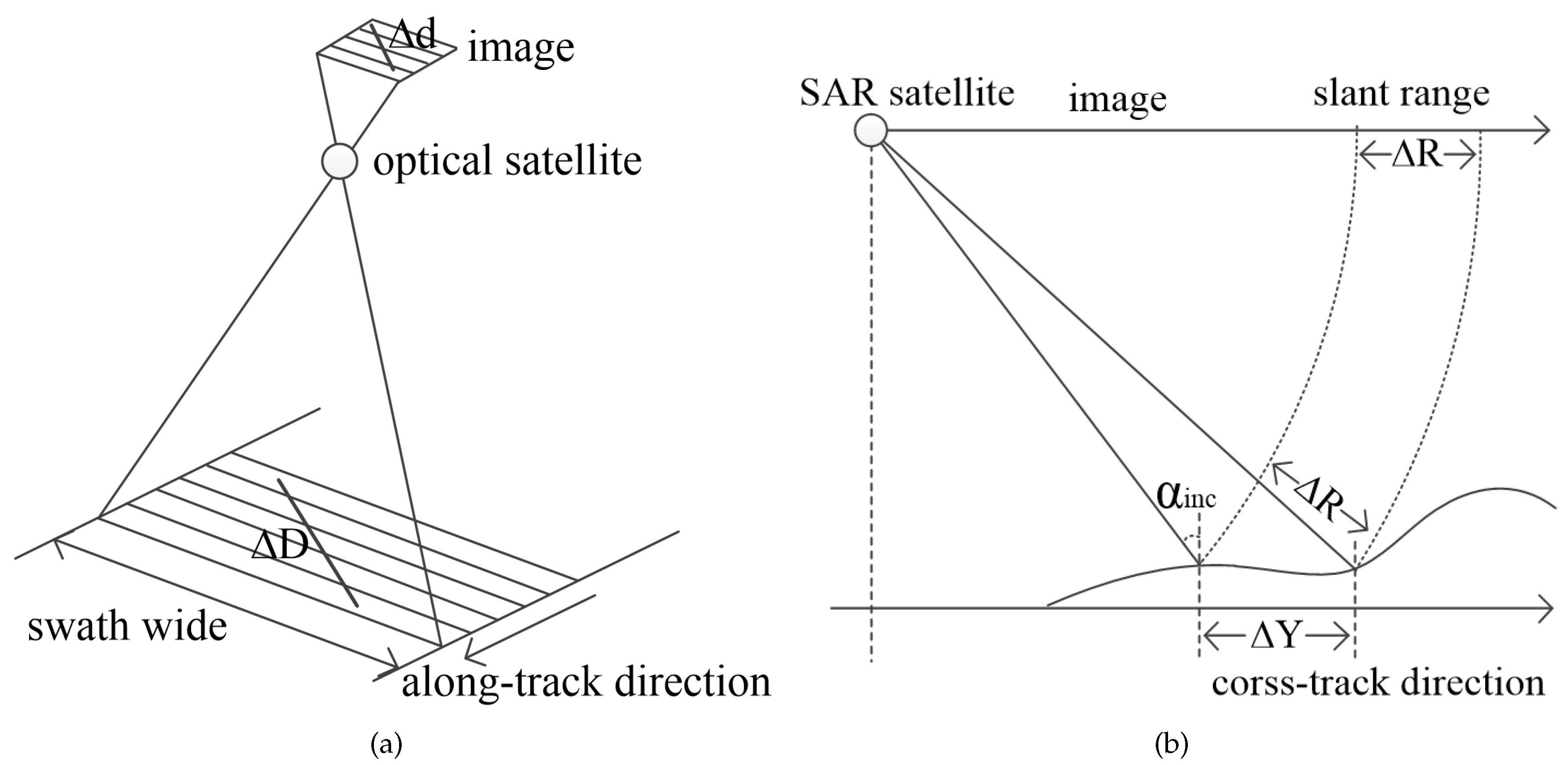
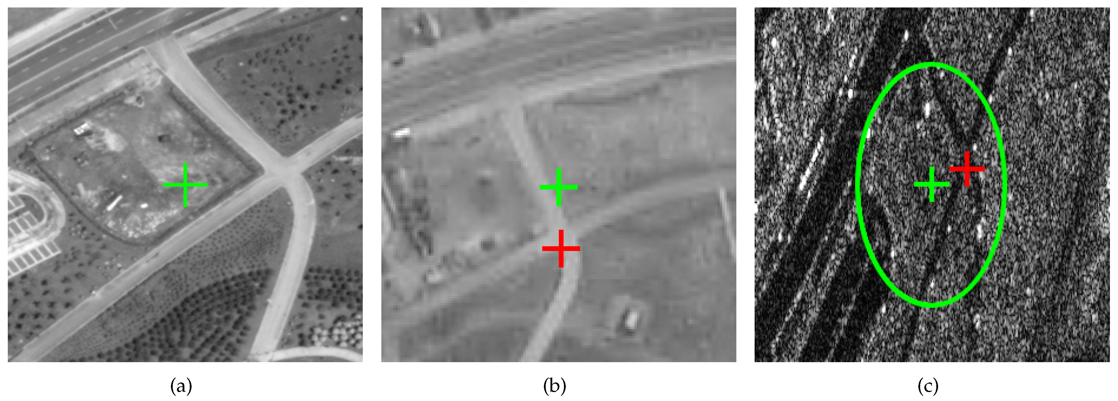
Remotesensing 12 00568 g001
Figure 2. The image point extraction for GLAS footprint: (a) digital orthophotograph model (DOM), (b) high-resolution (HR) optical image, and (c) synthetic aperture radar (SAR) image. The image points calculated by back-projection are indicated by a green cross. The final image points located in obvious texture area are indicated by a red cross. The circle footprint with a diameter of 70 m is marked by a green ellipse (the line resolution is 0.331 m and sample resolution is 0.562 m). The geometric accuracies of the used DOM, HR optical image, and SAR image were about 0.3, 30, and 5 m, respectively.
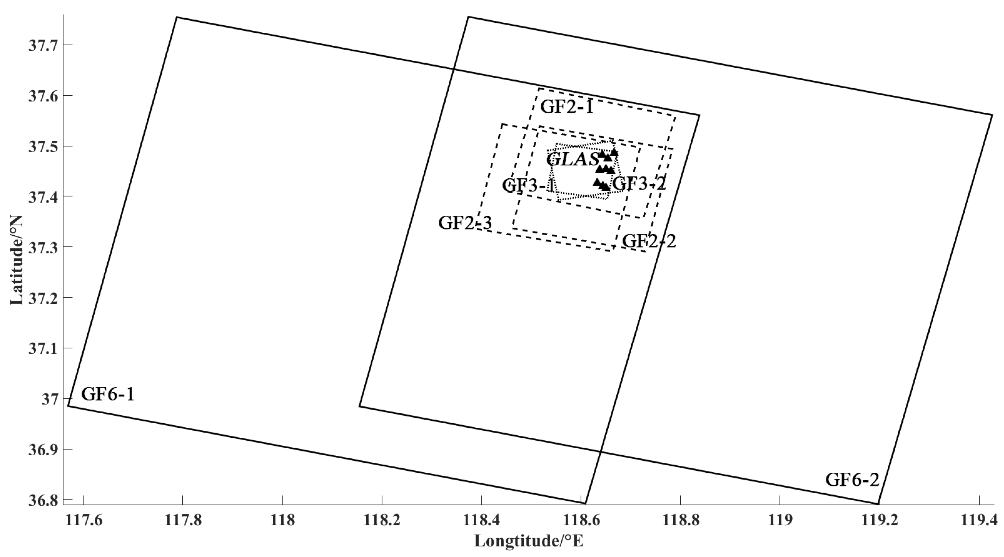
Remotesensing 12 00568 g002
Figure 3. An illustration of the coverage area of the experimental data.
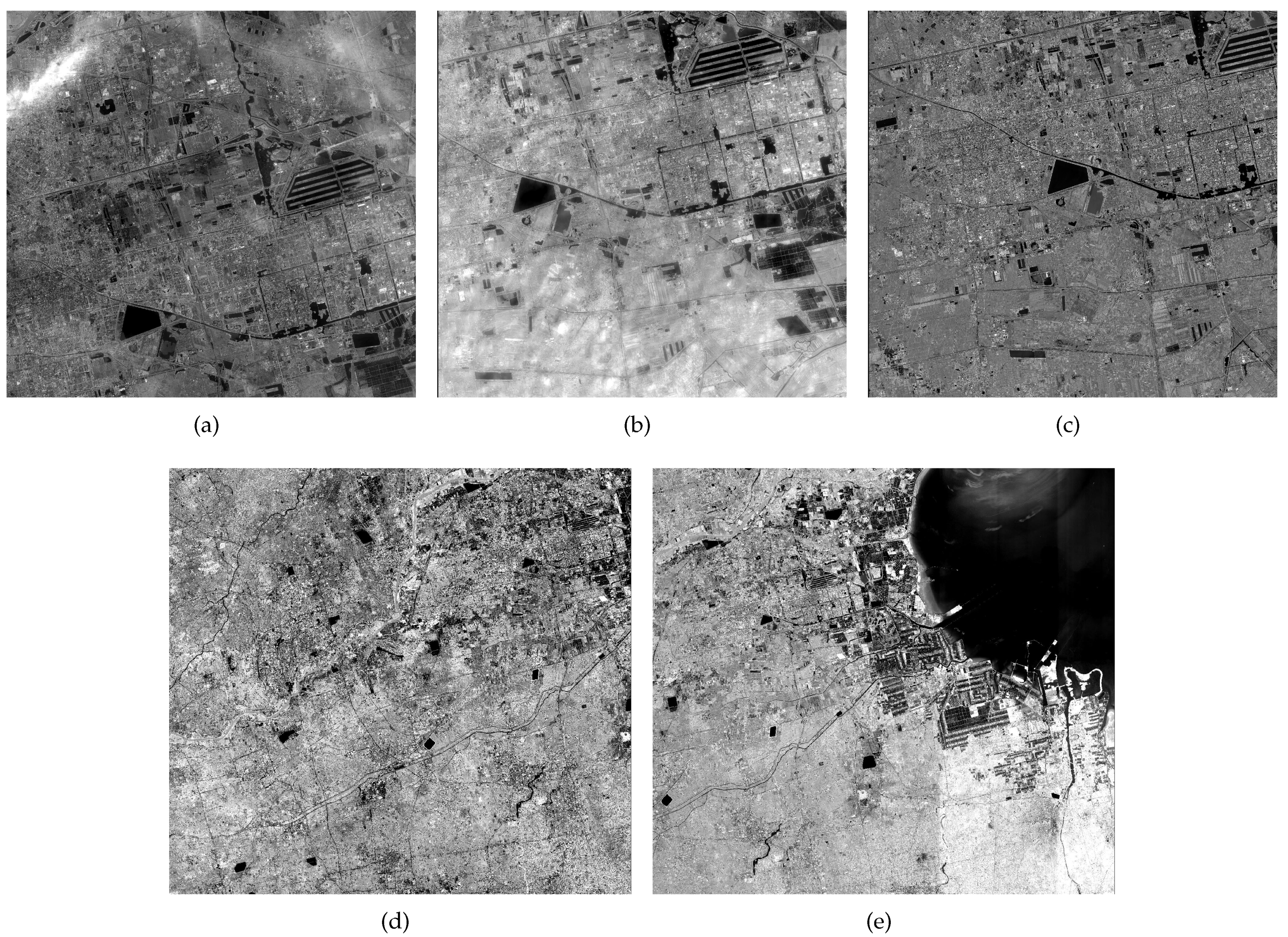
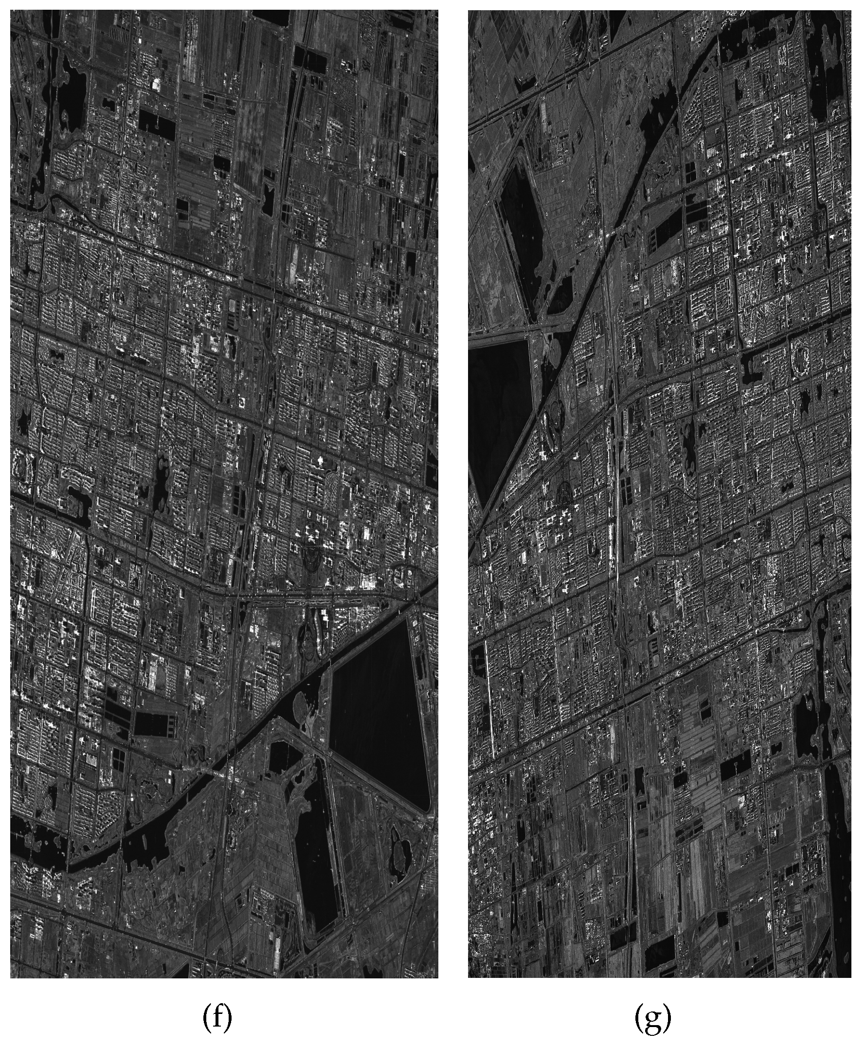
Remotesensing 12 00568 g003
Figure 4. Experimental data for combined geopositioning: (a) GF2-1, (b) GF2-2, (c) GF2-3, (d) GF6-1, (e) GF6-2, (f) GF3-1, and (g) GF3-2.
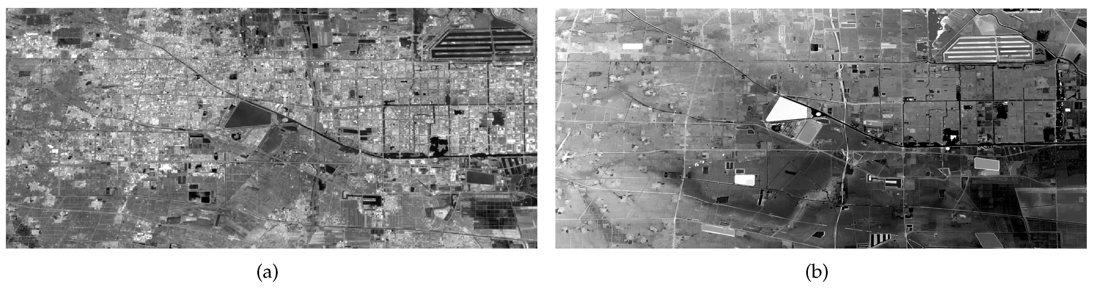
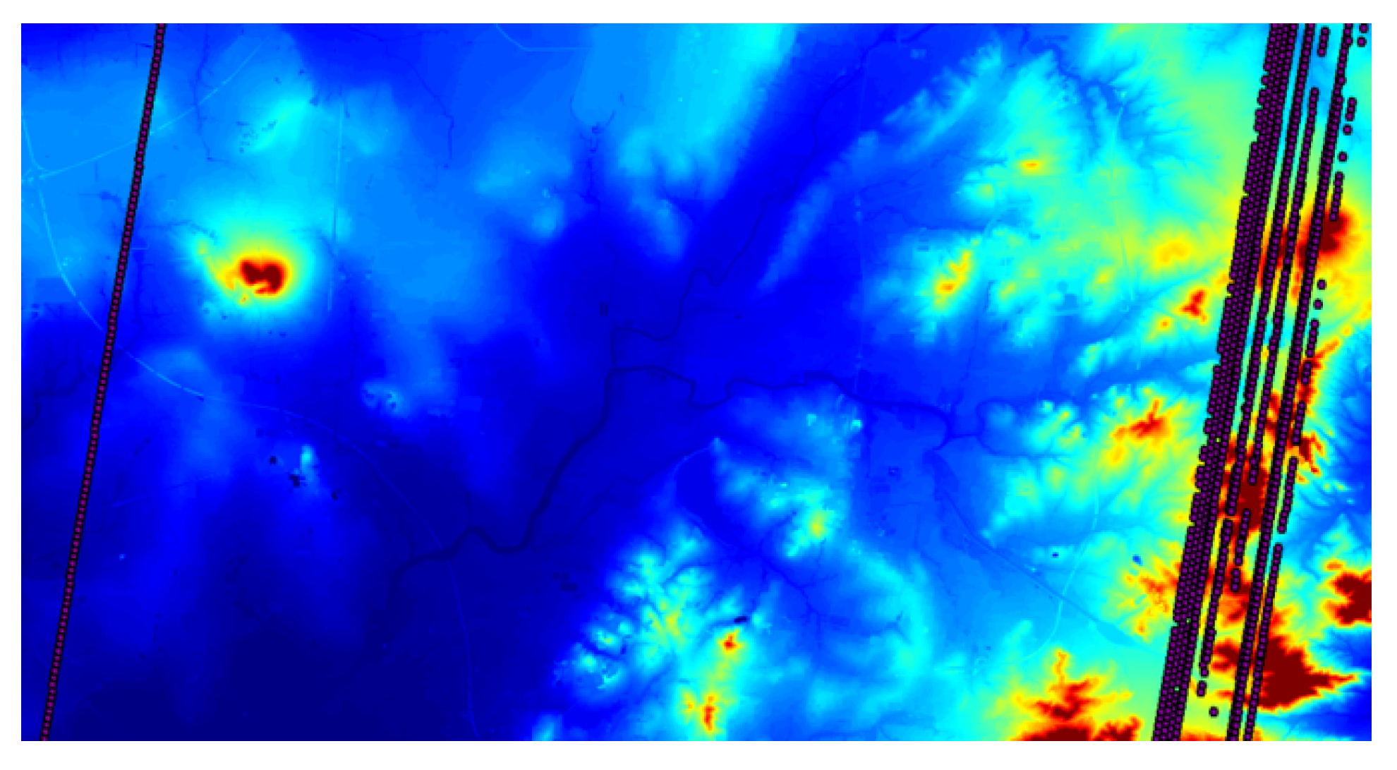
Remotesensing 12 00568 g004aRemotesensing 12 00568 g004b
Figure 5. The reference evaluation data: (a) DOM and (b) digital elevation models (DEM).
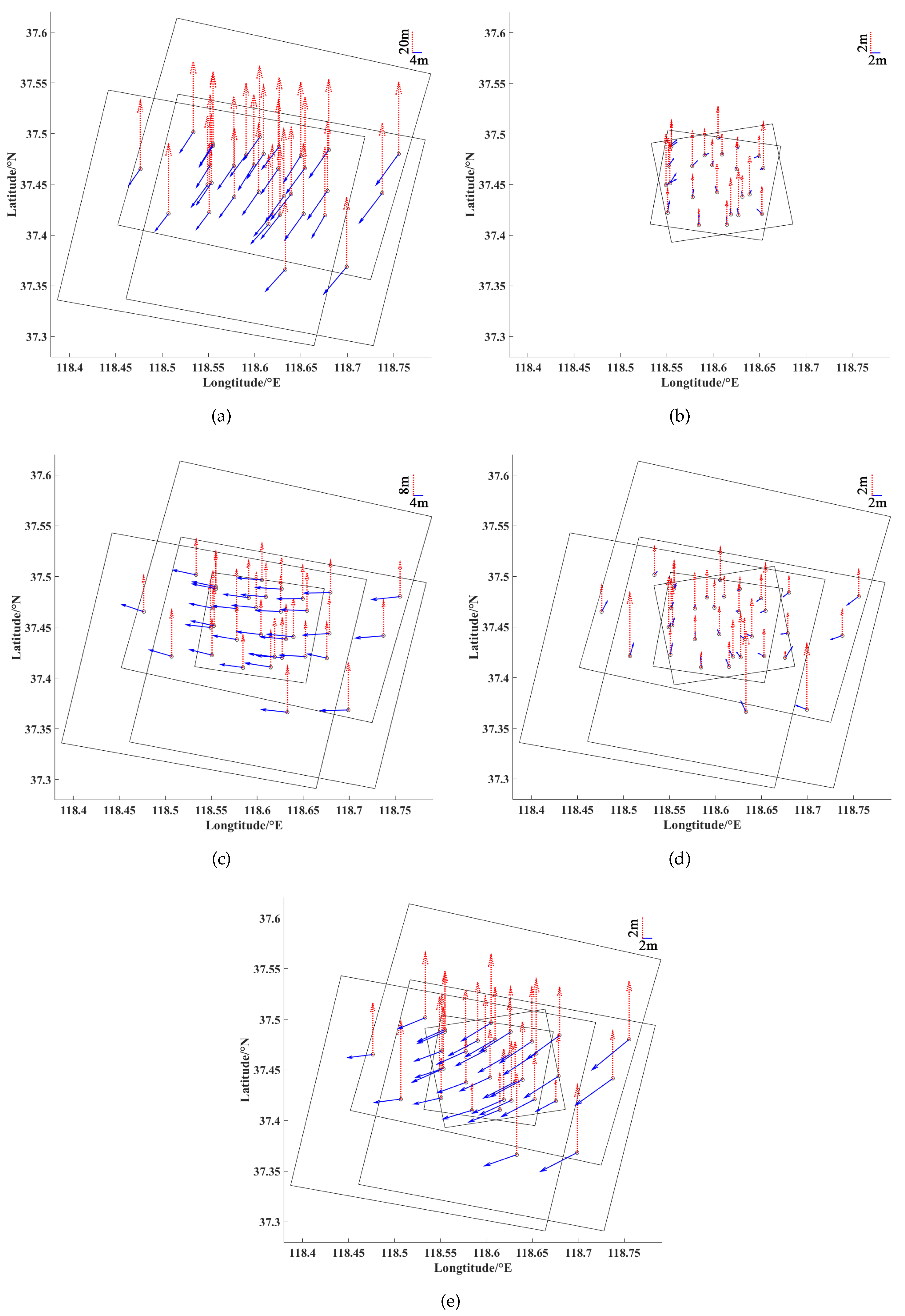
Remotesensing 12 00568 g005
Figure 6. 
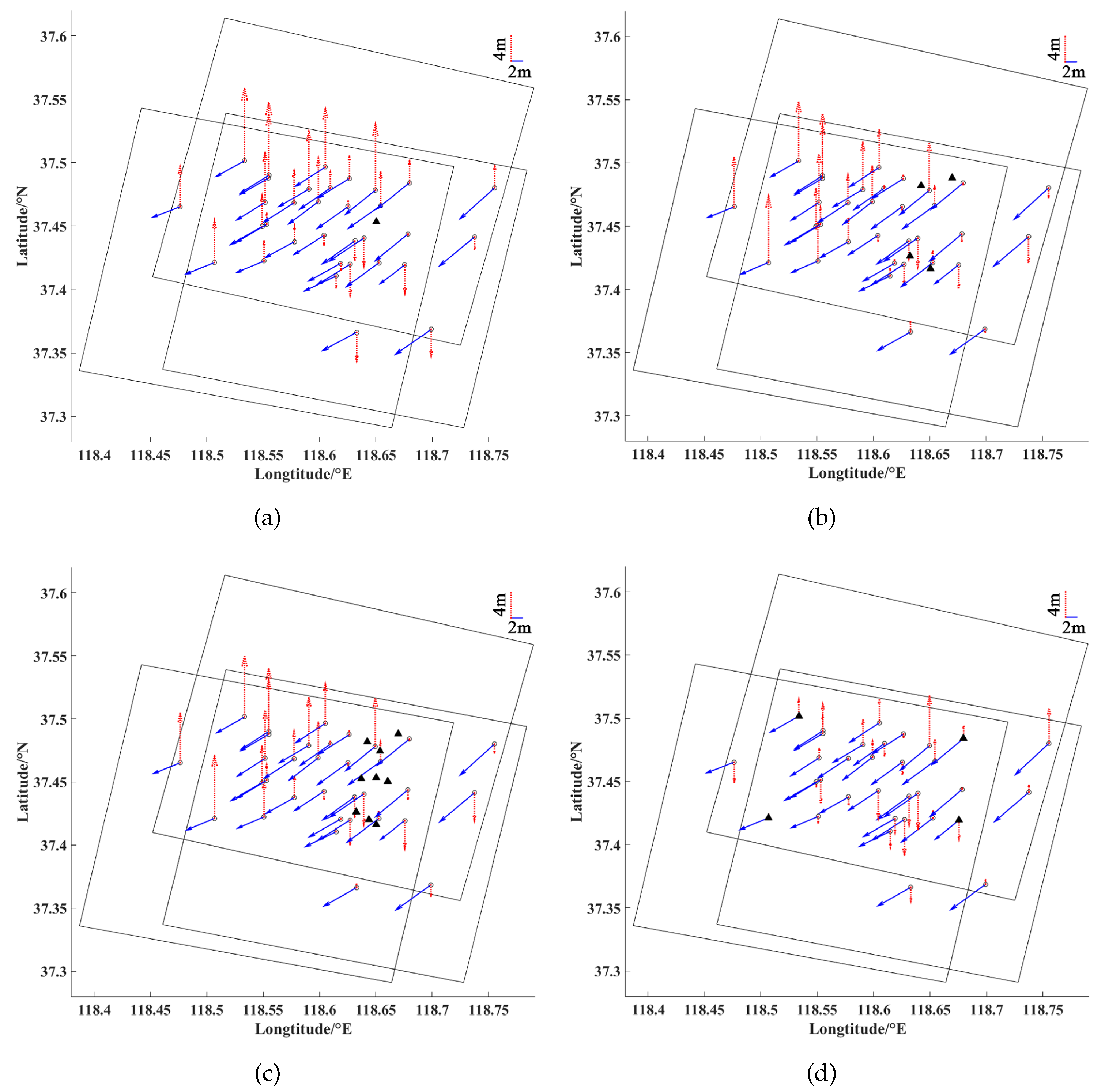
Geometric accuracy analysis of GF2 and GF3: (a) GF2 geopositioning, (b) GF3 geopositioning. (c) GF2 + GF3-1 combined geopositioning, (d) GF2 + GF3-1 + GF3-2 combined geopositioning, and (e) GF2 + GF3-1 + GF3-2 combined geopositioning with the same weight. Check points (CKPs) are represented by circles. The plane error and altitude error are represented by the vectors marked by the solid line and the dotted line, respectively.
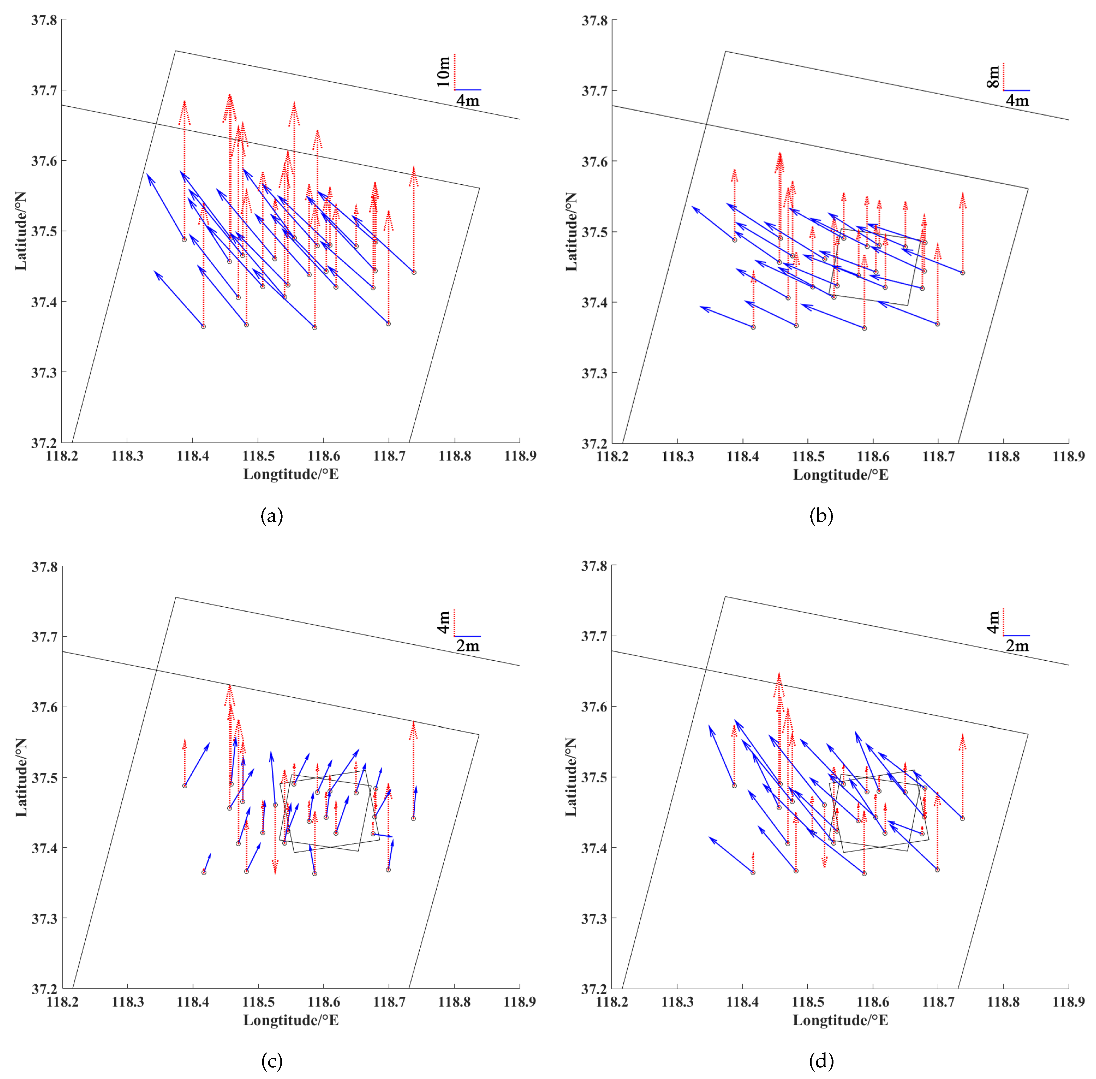
Remotesensing 12 00568 g006
Figure 7. 
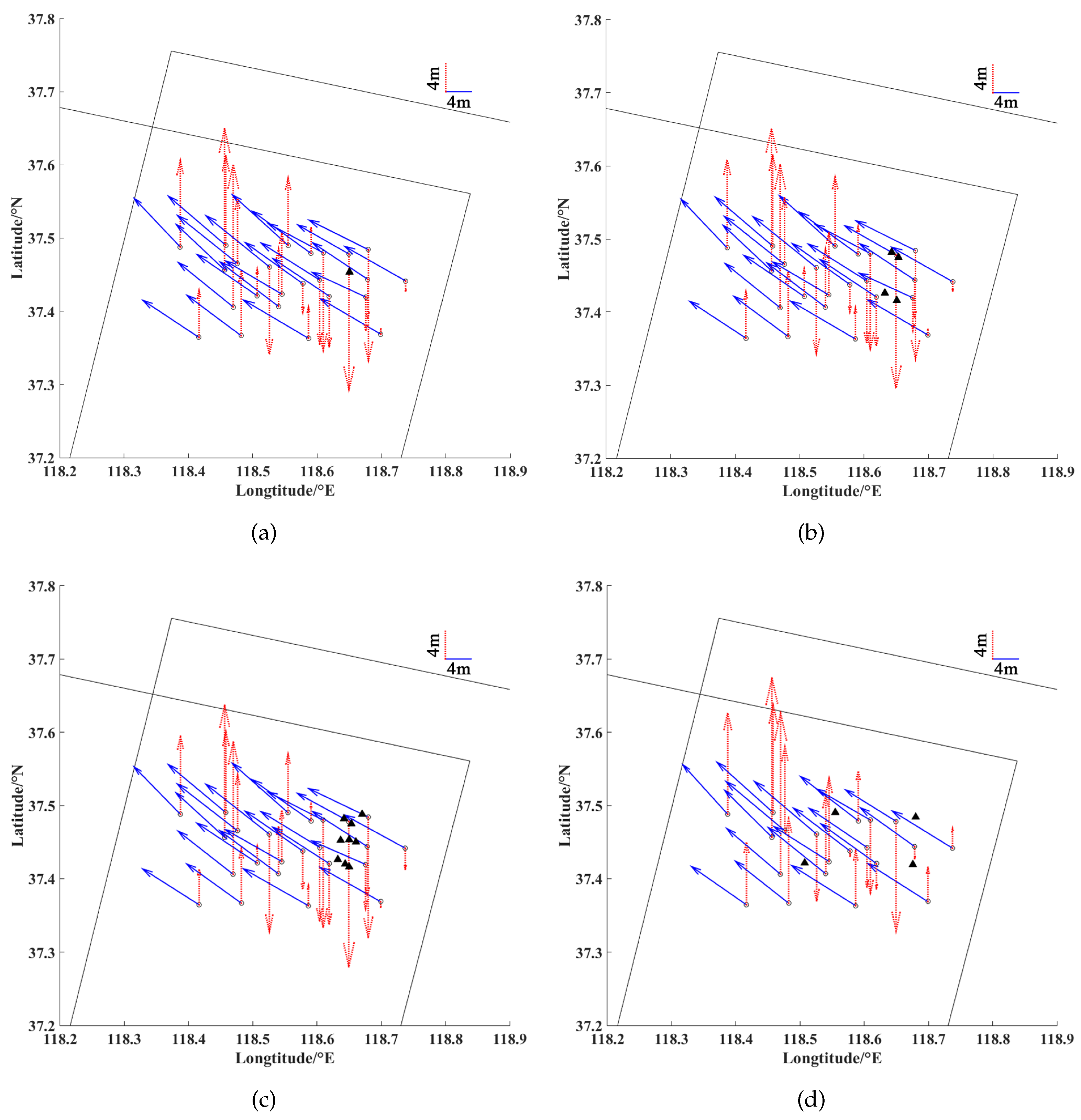
Geometric accuracy analysis of GF6 and GF3: (a) GF6 geopositioning, (b) GF6 + GF3-1 combined geopositioning, (c) GF6 + GF3-1 + GF3-2 combined geopositioning, and (d) GF6 + GF3-1 + GF3-2 combined geopositioning with the same weight.
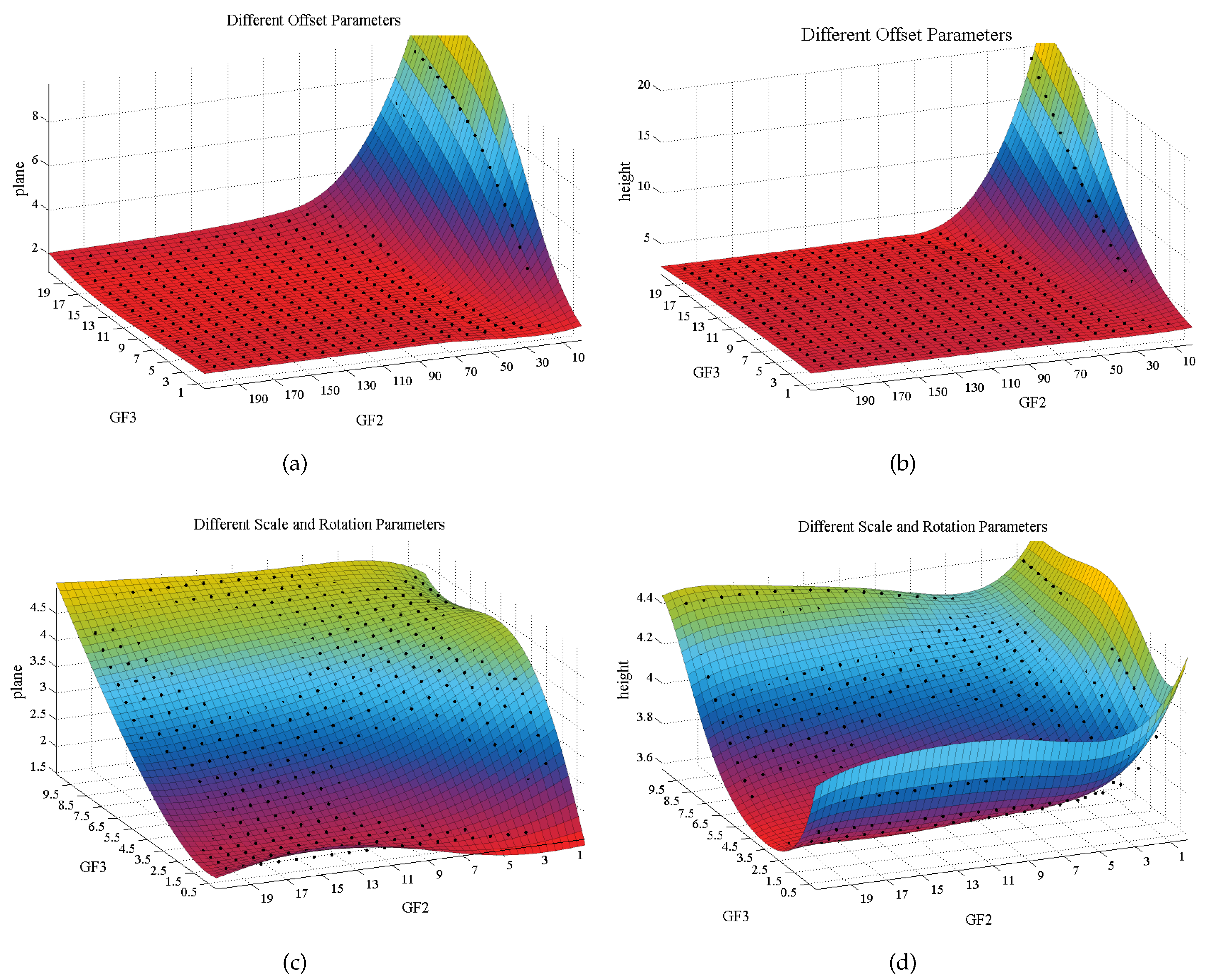
Remotesensing 12 00568 g007
Figure 8. Geometric accuracy analysis of GF2 and GF3 combined geopositioning: (a) plane geometric accuracy analysis with different offset parameters, (b) altitude geometric accuracy analysis with different offset parameters, (c) plane geometric accuracy analysis with different scale and rotation parameters, and (d) altitude geometric accuracy analysis with different scale and rotation parameters.
Remotesensing 12 00568 g008
Figure 9. Evaluation of the GLAS footprint extraction with the proposed criterion. The GLAS footprints are marked with red points.
Remotesensing 12 00568 g009
Figure 10. 
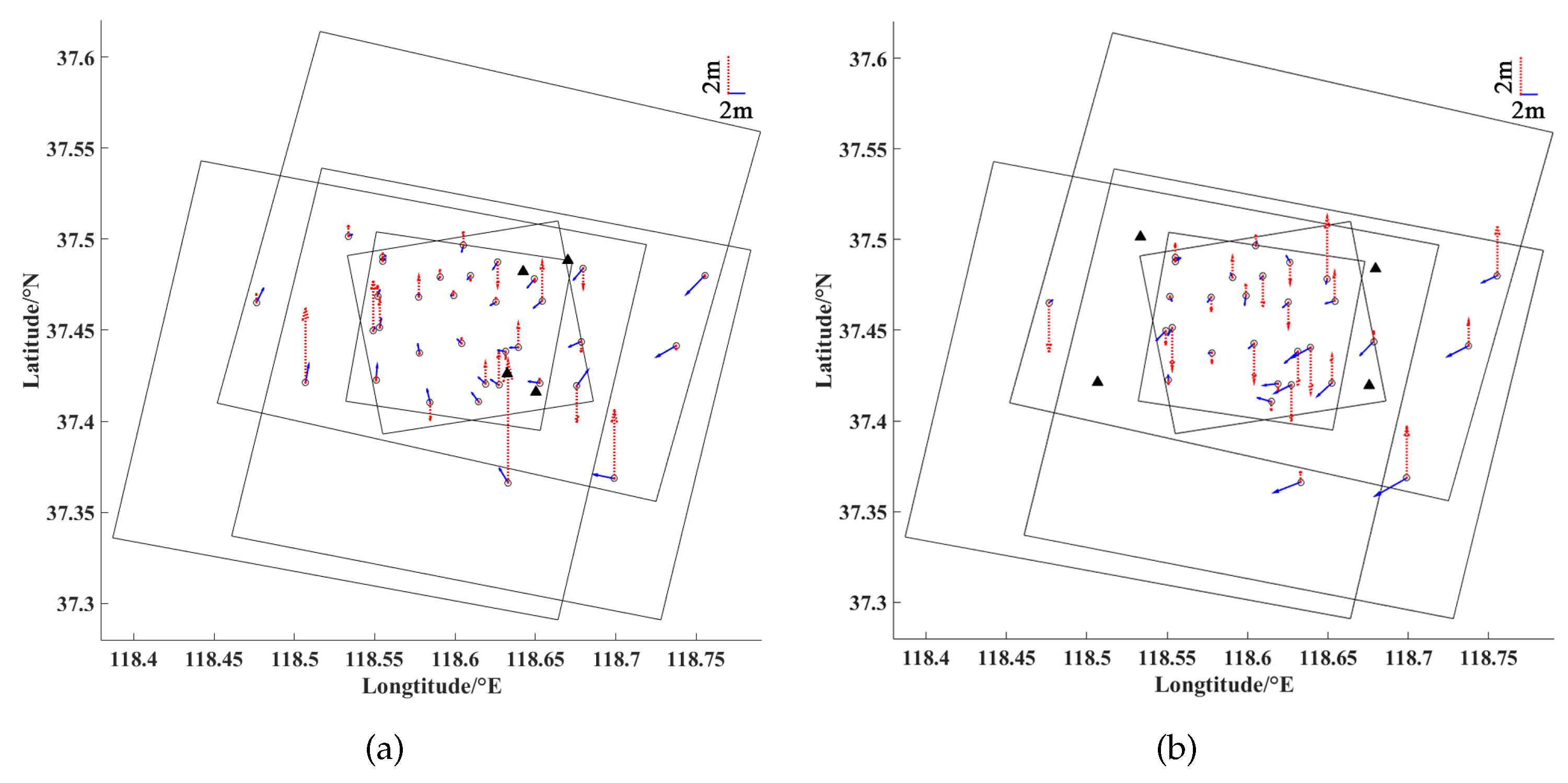
Geometric accuracy analysis of GF2 and GLAS combined geopositioning: (a) with one GLAS footprint, (b) with four GLAS footprints, (c) with nine GLAS footprints and (d) with four height control points. The GLAS footprints and height control points are represented as triangles. The plane error and altitude error are represented by the vectors marked with the solid line and the dotted line, respectively.
Remotesensing 12 00568 g010
Figure 11. 
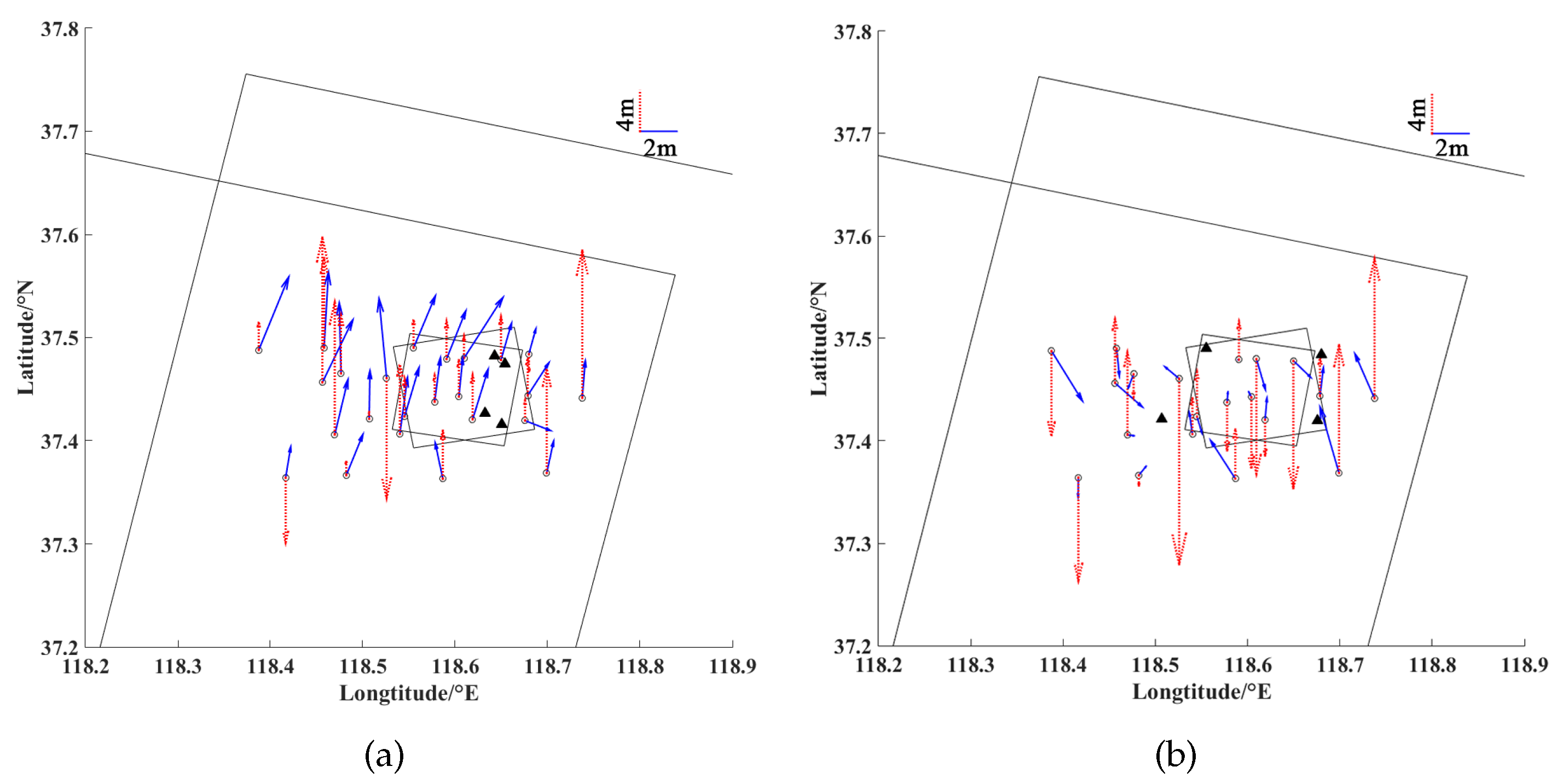
Geometric accuracy analysis of GF6 and GLAS combined geopositioning: (a) with one GLAS footprint, (b) with four GLAS footprints, (c) with nine GLAS footprints, and (d) with four height control points.
Remotesensing 12 00568 g011
Figure 12. Geometric accuracy improvement analysis: (a) GF3, GF3, and GLAS combined geopositioning and (b) GF2 with four GCPs.
Remotesensing 12 00568 g012
Figure 13. Geometric accuracy improvement analysis: (a) GF6, GF3, and GLAS combined geopositioning and (b) GF6 with four GCPs.
Remotesensing 12 00568 g013
Table 1. Geopositioning error sources of optical satellite and synthetic aperture radar (SAR) satellite.
ErrorError Source of Optical SatelliteError Source of SAR Satellite
Along-track offset errorTime error, along-track position error, pitch angle error, along-track detector errorsDrift error of spacecraft time, along-track position error, radial position error, velocity error
Along-track linear or scale errorLens distortion, focal length error, position error along the sub-satellite directionRelative error of stable local oscillator, along-track velocity error
Cross-track offset errorCross-track position error, roll angle error, cross-track detector errors, atmosphere refraction errorDelay error between signal transmitter and signal receiver, cross-track position error, radial position error, atmospheric delay
Cross-track linear or scale errorCross-track lens distortion, focal length error, position error along the sub-satellite directionIncident angle error, radial position error, atmospheric delay
Table 2. The criterion for Geoscience Laser Altimeter System (GLAS) footprint extraction.
CharacteristicCondition
Altitude difference compared with GDEM2<20
GLA01 productNumber of peaks of received waveform=1
Sigma of Gaussian of received waveform≤3.2
GLA14 productAttitude quality indicator=0
Surface reflectance parameter<1
Saturation correction flag=0
Table 3. Satellite parameters of GF2, GF6, and GF3.
GF2GF6GF3
Orbit altitude631 km644.5 kmOrbit altitude506 km
Orbit typeSunSyncSunSyncOrbit typeSunSync
Life5–8 years8 yearsLife8 years
B1: 450–520 nmB1: 450–520 nm
B2: 520–590 nmB2: 520–600 nm
Spectral rangeB3: 630–690 nmB3: 630–690 nmBandC
B4: 770–890 nmB4: 760–900 nm
Pan: 450–900 nmPan: 450–900 nm
Field of view ( )2.18.6Incident angle ( )10–60
Scanning angle ( )±20
Resolution (m)0.812Imaging modeSpotlight mode (1, 10 × 10)
Swath width (km)4590(Resolution (m),Hyperfine strip model (3, 30)
swath width (km))Fine strip mode 1 (5, 50)
Fine strip mode 2 (10, 100)
Standard strip model (25, 130)
Narrow scan mode (50, 300)
Wide scan mode (100, 500)
Full polarization strip model 1 (8, 30)
Full polarization strip model 2 (25, 40)
Wave imaging mode (10, 5 × 5)
Global observation model (500, 650)
Extended incident angle model (25, 130 or 80)
Table 4. Description of experimental data for combined geopositioning.
ImageAcquisition DatePassIncident Angle ( )Size (pixels)Resolution (m)
GF2-12 February 2015DEC15.50229,200 × 27,6200.81 × 0.81
GF2-221 September 2015DEC−8.40329,200 × 27,6200.81 × 0.81
GF2-326 August 2016DEC−12.44429,200 × 27,6200.81 × 0.81
GF6-113 March 2019DEC−0.00444,500 × 48,3122 × 2
GF6-217 March 2019DEC−0.00344,500 × 48,3122 × 2
GF3-19 April 2017DEC43.796–44.34230,642 × 13,5440.34 × 0.56
GF3-216 April 2017ASC39.224–39.88133,760 × 13,3820.33 × 0.56
Reference dataResolution (m)Accuracy (m)Range
DOM0.2710.251Lat: 37.3408–37.5170
DEM1.8060.273Lon: 118.3691–118.8056
Table 5. Geometric accuracy of GF2, GF3, and GLAS combined geopositioning.
Experimental DataAverageRMSE (m) MAX (m)
Convergent Angle ( )PlaneAltitude PlaneAltitude
AGF218.63013.08575.857 17.48980.069
GF373.1401.5323.272 2.6845.597
GF2 + GF3-127.64411.97716.095 13.76320.732
GF2 + GF3-1 + GF3-234.8451.7243.784 3.2798.903
GF2 + GF3-1 + GF3-2 (with the same weight)34.8458.1076.061 11.1918.952
BGF2 + one GLAS footprint-14.1293.208 17.5076.404
GF2 + four GLAS footprints-13.8902.865 17.4105.842
GF2 + nine GLAS footprints-13.9452.882 17.4475.560
GF2 + four height control points-13.9741.805 17.2644.367
CGF2 + GF3 + four GLAS footprints-1.5871.985 3.4557.424
GF2 + four control points-1.9451.803 4.8853.789
Table 6. Geometric accuracy of GF6, GF3, and GLAS combined geopositioning.
Experimental DataAverageRMSE (m) MAX (m)
Convergent Angle ( )PlaneAltitude PlaneAltitude
AGF65.1612.87835.901 14.64353.549
GF6 + GF3-126.2010.07920.524 11.65434.517
GF6 + GF3-1 + GF3-237.432.8239.186 4.13119.543
GF6 + GF3-1 + GF3-2 (with the same weight)37.435.2809.528 7.14320.989
BGF6 + one GLAS footprint-11.57011.542 13.40021.641
GF6 + four GLAS footprints-11.55811.519 13.38821.710
GF6 + nine GLAS footprints-11.51211.418 17.4475.560
GF6 + four height control points-11.62012.490 13.41424.435
CGF6 + GF3 + four GLAS footprints-2.9087.669 4.34315.877
GF6 + four control points-1.7379.290 3.76120.144
Table 7. Geometric accuracy with different offset parameters for GF2 and GF3 combined geopositioning. The first column relates to GF2 and the first row relates to GF3.
1351020
PlaneAltitudePlaneAltitudePlaneAltitudePlaneAltitudePlaneAltitude
101.8023.7202.1354.0353.2774.6996.5997.9529.30419.376
301.8233.7321.7433.7471.7243.7842.2323.9705.4324.854
501.8393.7351.7663.7271.7203.7161.7183.6703.7273.538
1001.8473.7361.7803.7181.7363.6861.6163.5472.6693.018
1501.8483.7371.7833.7171.7403.6821.6113.5252.4882.926
2001.8493.7371.7843.7161.7423.6811.6113.5172.3302.895
Table 8. Geometric accuracy with different scale and rotation parameters for GF2 and GF3 combined geopositioning.
0.512510
PlaneAltitudePlaneAltitudePlaneAltitudePlaneAltitudePlaneAltitude
11.5884.5501.7184.2102.1444.0423.3964.1994.1154.346
31.6074.2891.6434.0091.8623.8252.8723.8923.9514.113
51.6594.2321.6613.9751.7483.7862.4153.7723.6323.997
101.7074.2061.7073.9681.7243.7841.9763.6903.0373.841
151.7194.2021.7233.9681.7383.7901.8563.6582.7503.749
201.7234.2001.7303.9691.7463.7931.8083.6372.6003.669
Table 9. GLAS footprint extraction with the proposed criteria.
CriterionNumber of DataMean (m)RMSE (m)
Original data5312−4.49016.060
With GDEM2 <205064−1.2532.799
With GDEM2 <20 and criterions in GLA14 product3257−1.3392.615
With GDEM2 <20 and criterions in GLA01 product3419−0.8652.049
With GDEM2 <20 and criterions in GLA14 and GLA01 products2272−0.9191.969

