Impacts of Land Cover/Use on the Urban Thermal Environment: A Comparative Study of 10 Megacities in China


1
Graduate School of Life and Environmental Sciences, University of Tsukuba, 1-1-1 Tennodai, Tsukuba 305-8572, Ibaraki, Japan
2
Institute of Ecological Civilization, Jiangxi University of Finance and Economics, Nanchang 330013, China
3
Faculty of Life and Environmental Sciences, University of Tsukuba, 1-1-1 Tennodai, Tsukuba 305-8572, Ibaraki, Japan
*
Author to whom correspondence should be addressed.
Remote Sens. 2020, 12(2), 307; https://doi.org/10.3390/rs12020307
Submission received: 10 December 2019
/
Revised: 10 January 2020
/
Accepted: 13 January 2020
/
Published: 17 January 2020
(This article belongs to the Special Issue Geospatial Analysis of Urban Heat Island Phenomena in Megacities)
Abstract
:Satellite-derived land surface temperature (LST) reveals the variations and impacts on the terrestrial thermal environment on a broad spatial scale. The drastic growth of urbanization-induced impervious surfaces and the urban population has generated a remarkably increasing influence on the urban thermal environment in China. This research was aimed to investigate land surface temperature (LST) intensity response to urban land cover/use by examining the thermal impact on urban settings in ten Chinese megacities (i.e., Beijing, Dongguan, Guangzhou, Hangzhou, Harbin, Nanjing, Shenyang, Suzhou, Tianjin, and Wuhan). Surface urban heat island (SUHI) footprints were scrutinized and compared by magnitude and extent. The causal mechanism among land cover composition (LCC), population, and SUHI was also identified. Spatial patterns of the thermal environments were identical to those of land cover/use. In addition, most impervious surface materials (greater than 81%) were labeled as heat sources, on the other hand, water and vegetation were functioned as heat sinks. More than 85% of heat budgets in Beijing and Guangzhou were generated from impervious surfaces. SUHI for all megacities showed spatially gradient decays between urban and surrounding rural areas; further, temperature peaks are not always dominant in the urban core, despite extremely dense impervious surfaces. The composition ratio of land cover (LCC%) negatively correlates with SUHI intensity (SUHII), whereas the population positively associates with SUHII. For all targeted megacities, land cover composition and population account for more than 63.9% of SUHI formation using geographically weighted regression. The findings can help optimize land cover/use to relieve pressure from rapid urbanization, maintain urban ecological balance, and meet the demands of sustainable urban growth.

1. Introduction
The United Nations (UN) portrays the 21st century as an urban age because of a substantial increase in the urban population across the globe, in which more than 55% of humans came to live in urban settings [1]. The growth and densification of the urban population have given rise to a drastic urban expansion, as well as a range of negative impacts, including the urban heat island (UHI) phenomenon. UHI, which initiates higher ambient temperature in the urban core than in neighboring rural areas due to speedy urbanization [2], engenders high ecological pressure and risk on the local terrestrial ecosystem [3]. In this connection, science programs have been devoted to studying the relationship between the human system and the thermal environment at local and global levels [4]. Achieving urban sustainability and easing urban climate problems have been given priority under Goals 11 and 13 of the 17 Sustainable Development Goals (SDGs) issued by the UN in 2015 [5]. Therefore, as an indispensable actor in global urbanization, China places a high premium on these issues, which can help “make cities inclusive, safe, resilient, and sustainable” [5,6,7].
Notably, China has undergone swift, massive urbanization since the 1990s, its urbanization rate increased from 25.84% to 49.68% between 1990 and 2010 [8]. The results of satellite monitoring show that China witnessed an expansion of its built-up area from 12,252.9 km2 in 1990 to 40,533.8 km2 in 2010 [8,9]. Urban zones in China have seen explosive growth in the early 21st century, mainly in the eastern plains [9,10,11,12]. This implies that East China is especially sensitive to urban environmental vulnerability and ecological sustainability issues given its context of rapid urbanization. East China faces very high urban ecosystem risks and is in urgent need of mitigation solutions, especially regarding UHI.
Partly as a result of this urgency, numerous investigations of China’s thermal environment have been carried out [13,14,15,16,17,18]. Satellite data have been used to detect thermal differences between urban and rural surfaces across the country [13,19,20,21,22,23,24]. As addressed in existing thermal environment studies, the stronger thermal effects of urbanization are often found in the cities or densely populated regions [11,12], e.g., Beijing [25,26], Guangzhou [11], Nanjing [27], and Wuhan [28]. These cities have been frequently examined and have experienced substantial UHI over several decades [16,20]. In major Chinese cities, the UHI footprint has shown a significantly decaying gradient from the urban center toward neighboring rural areas [18]. Surface UHI (SUHI) is associated with the relative “temperature cliff” between metropolitan and rural regions. The driving forces behind the “temperature cliff” in China’s urban-rural zones are also very significant [17]. A considerable degree of urban population accommodation and migration, as well as drastic urban land transitions—which have led to the dominance of impervious surfaces (ISs) and degraded cultivated land—have given rise to various climate ramifications, exacerbating UHI [12,15,29,30]. Therefore, it is pivotal to provide comprehensive, scientific insight into the status and mechanism of the urban thermal environment in China.
Geographers have long utilized several kinds of spatial or statistical methods to testify to the causality between land cover types and SUHI [4]. Most SUHI studies have employed Pearson’s correlation, along with different indexes, quantifying the causal relationship using data from a single location or a continuous area [4,20]. Although these findings are critical for understanding the UHI effect and influencing factors, the application of these methods would be obstructed when spatial datasets are used, or spatial relationships are investigated. In contrast, we used the geographically weighted regression (GWR) model, which can illustrate spatial non-stationarity, permitting us to observe significant total and local variation and thus determine the statistical significance of an explanatory variable [21,31,32,33,34]. Several studies have already clarified the quantitative relationships between the UHI effect and its potential influencing factors based on GWR [4]. Zhao et al. [32] investigated the spatial heterogeneity of the relationships between underlying surface characteristics and SUHI. Li et al. [35] suggested that both the population and land cover/use fraction (e.g., greenspace) significantly affect the status of SUHI. In this study, we hypothesized statistically significant causality among UHI (effect), land cover types (cause I), and population (cause II) in multiple Chinese megacities.
Stretching across a vast territory, China has witnessed a significant imbalance in the development of different regions, and the urban environmental issues are complicated and manifolded. The region in the east of Heihe-Tengchong Line covers 43% of the national land extending from tropical, subtropical, to temperate climate zones, where 94% of Chinese citizens reside [36]. Widespread from tropical cities [37], mountain cities [38], humid cities [11], to coastal cities [39], the evaluations of the urban thermal environment in the Chinese megacities are usually considering multiple aspects [40,41]. Thus, in recent decades, UHI-related research has often analyzed only a single city. It is a great challenge to comprehensively assess and compare the impact of the UHI effect on multiple Chinese megacities. However, there is an increasing trend shifting toward researching multiple cities, or even urban agglomerations, accompanying the enhancement of urban environmental conservation measures and the rising environmental awareness [12,42]. Nevertheless, the urban thermal field is significantly affected by multiple factors, especially atmospheric conditions [4]; thus, it is challenging to examine and compare thermal variation on the land surface across multiple dates and locations [43]. Previously, large-scale or multi-location UHI studies have utilized weather station data and images from the Moderate Resolution Imaging Spectroradiometer (MODIS) satellite, but have rarely employed Landsat images [4,20].
In this context, we investigate whether the appearance of a relative “temperature cliff” from urban to rural areas is primarily caused by anthropogenic heat variation, which is associated with differences due to human-dominated land cover/use composition and population distribution. The assessments of thermal environmental quality call for an in-depth land-population-oriented investigation based on land cover/use layout and configuration [3,4]. Unlike previous SUHI investigations, we carried out a multi-city comparative analysis using diverse spatial data (temperature, land cover, and population), targeting ten densely populated cities in China. These cities are not only the most advanced, populated, and vibrant megalopolises in China urbanization, but also the most urgent and critical regions for China’s ecological security. Their SUHI footprints would be scrutinized on the basis of both extent and magnitude, using diverse techniques. The spatial causal mechanisms among SUHI, land cover, and population in these diverse Chinese megalopolises are also studied using the GWR model.
The objectives of this study were to (1) investigate the spatial characteristics of the land surface temperature (LST) response to urban land cover based on Landsat monitoring, (2) estimate the SUHI footprint (SUHI intensity, abbreviated as SUHII), (3) identify the impacts of urban land cover configuration and population distribution on the thermal environment, and (4) create a sustainable strategy for UHI mitigation and the future development of Chinese cities.
2. Materials and Methods
2.1. Study Area Selection
In the wake of intensive urbanization-induced human activities, land surface transitions and urban expansion have exerted an enormous impact on the thermal environment of densely populated cities. Thus, there are strong incentives to synthetically and scientifically examine the linkages between UHI and the geographical process.
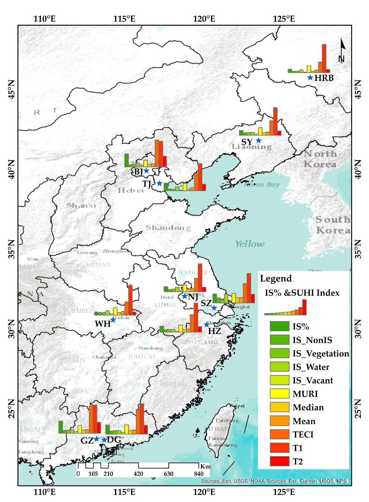
Several essential characteristics were used to decide this study’s area based on official Chinese census data from 2016, including (a) large population (over 5 million permanent residents), (b) regional terrain and climate, (c) frequent heatwaves over the decade, and (d) Landsat 8 data availability. Thus, the target includes Beijing (BJ), Dongguan (DG), Guangzhou (GZ), Hangzhou (HZ), Harbin (HRB), Nanjing (NJ), Shenyang (SY), Suzhou (SZ), Tianjin (TJ), and Wuhan (WH), as shown in Figure 1.
Beijing, located in the Jing-Jin-Ji urban agglomeration, is home to 21.705 million residents and is one of the most populous capital cities in the world. Dongguan and Guangzhou are neighbors, located in the Pearl River Delta, and their population densities are 3355 and 1816 people per km2, respectively. Hangzhou lies in the Zhejiang Greater Bay Area, with 9.02 million residents. Situated in the metropolitan area of Ha-Chang in Northeast China, Harbin has 9.61 million people and serves as a regional hub for politics, economics, culture, and industry. Nanjing plays a vital role in the urban agglomeration of the Yangtze River Delta, with 8.24 million inhabitants. Shenyang, with 6.3 million urban people, is located in the Mid-Southern Liaoning Metropolitan Area. Including its surroundings, Shenyang has a total population of 8.3 million. Suzhou, a prominent city in the Yangtze River Delta, is located on the lower reach of the Yangtze River, with 6.67 million inhabitants. Tianjin, one of the most famous coastal metropolises in Northern China, has 15.47 million inhabitants and serves as an important seaport and gateway to Beijing. Wuhan, situated in the Hubei Yangtze River Mid-Reaches Metropolitan Region, is the largest city in Central China, with 10.61 million people [8].
For the sake of comparative analysis, it is necessary to define an urban extent for each city. Each city consists of an 80 × 80 km landscape with a 40 km radius from the nearest city center, allowing us to distinguish temperature variation between urban and surrounding areas easily. The city center is located at the municipal government offices.
2.2. Data Description and Methodology
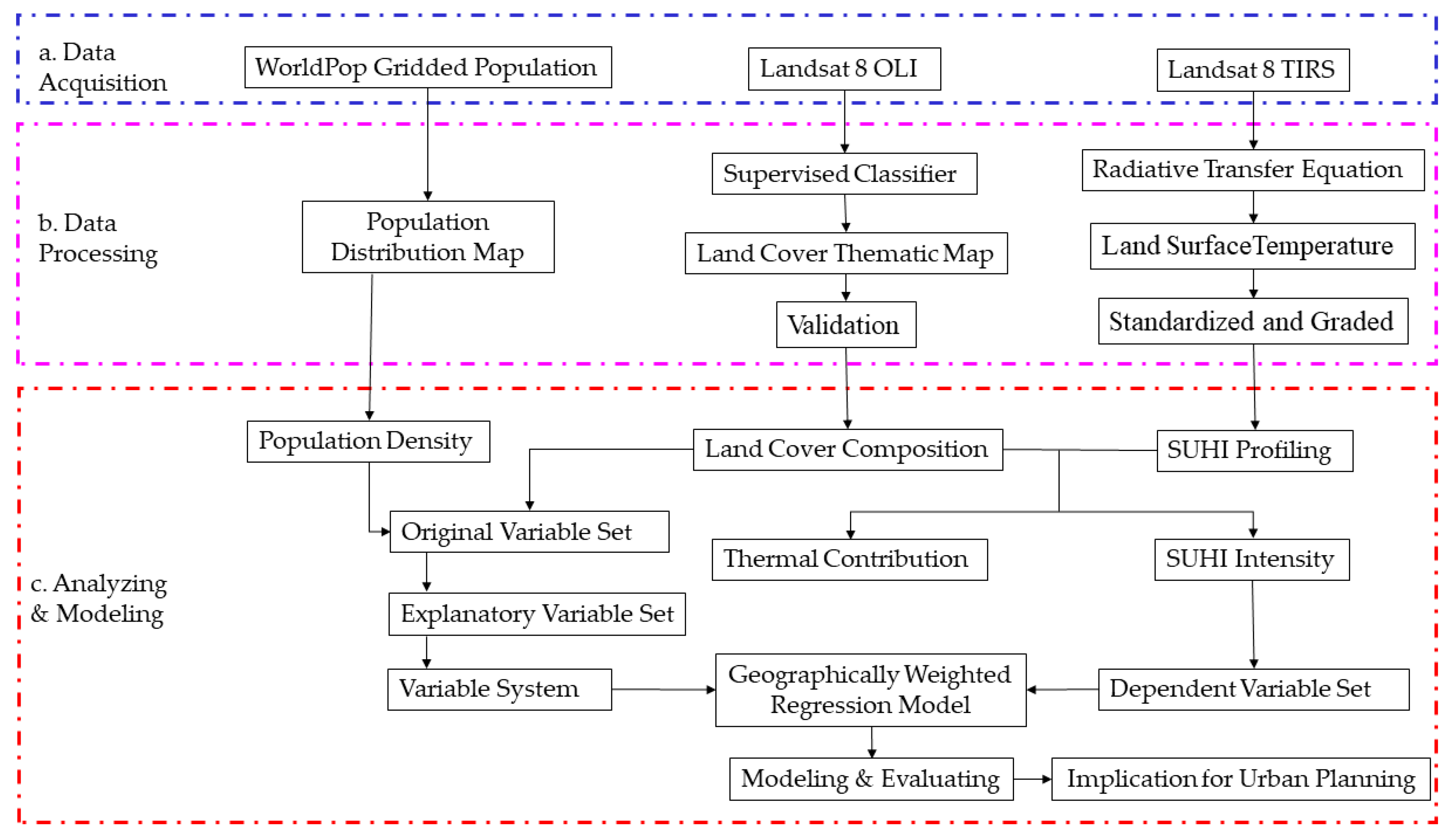
A general process for multi-city analysis of the SUHI footprint in Chinese megacities is implemented as shown in Figure 2. Three stages—(a) data acquisition, (b) data processing, and (c) analyzing and modeling—are designed. The specific technical methods and processes are illustrated as follows:
2.2.1. Spatial Distribution of Population
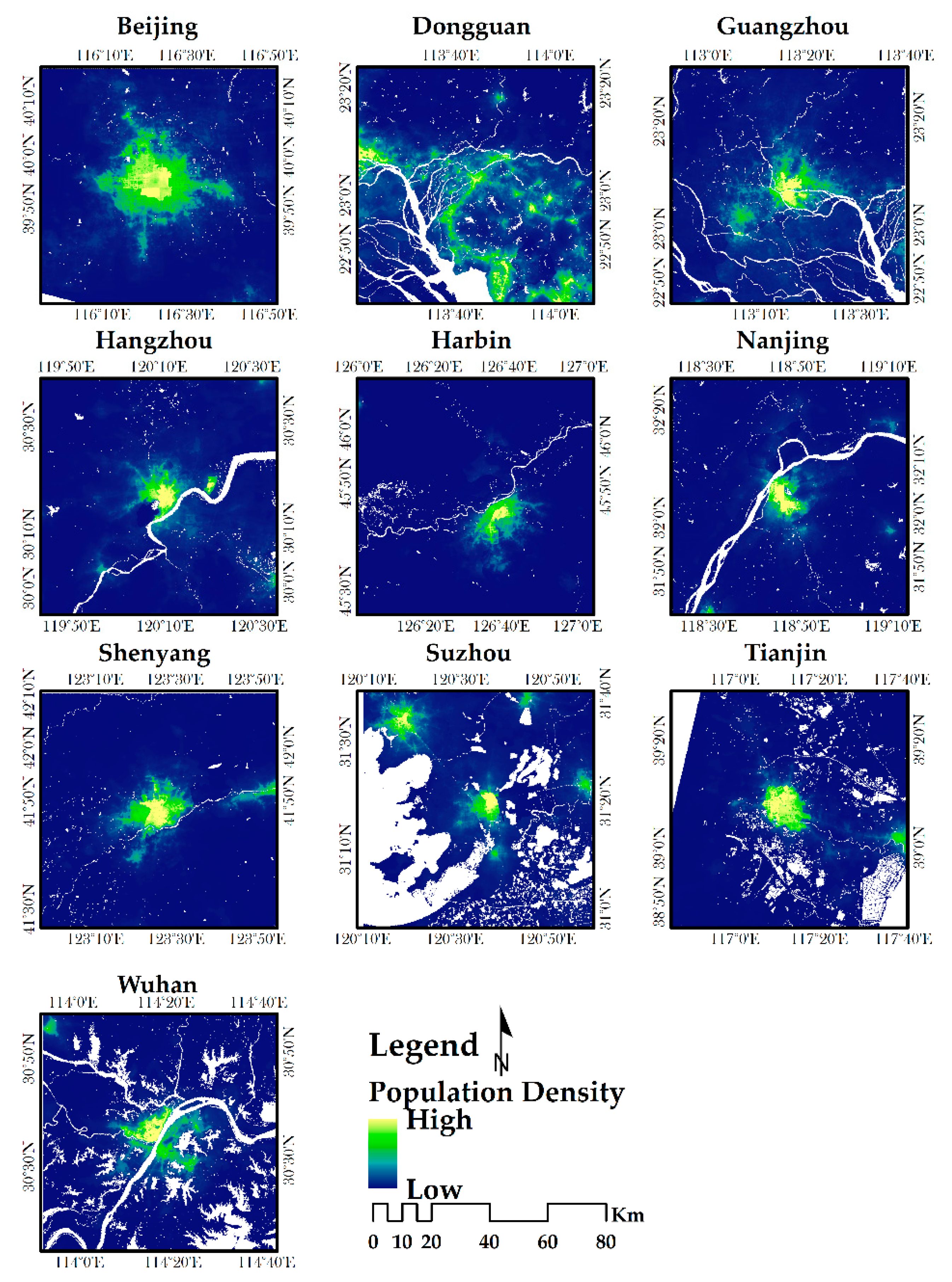
Dense human activities are one of the underlying causes of thermal field variations. Rapid urbanization has led to remarkable differences in underlying city surfaces, such as a substantial expansion of settlements and dwellings, both horizontally and vertically [44]. Thus, the information of accurate human population distribution is crucial to identify the impacts of human–thermal environment interactions. In this study, we utilized spatial demographic data from the 2015 Grid Population Dataset of China, with a spatial resolution of decimal degrees (approximately 100 m at the equator), found at WorldPop (www.worldpop.org), an open-access, country-level population database. Recently, data from WorldPop have been widely employed to support population-related investigations [45,46,47]. WorldPop mapped and visualized information from the national census using the random forests model with multi-source data, and adjusted it to match UN population division estimates [47]. Based on the result, we used 10 population distribution maps (Appendix Figure A1) extracted from the 2015 Grid Population Dataset of China, to conduct a spatial investigation of the respective population’s impacts on the thermal environment in each study region.
2.2.2. Land Cover/Use Mapping
A total of 10 land use and land cover (LULC) thematic maps were yielded for each city using an interactively supervised, maximum likelihood classifier through the software application ENVI 5.3. The maximum likelihood method is the most representative and useful pixel-based parametric classifier that delineates the LULC distribution using remote sensing imageries [48]. This method would perform well with sufficient training samples, and provide a valuable LULC thematic map based on a normality assumption and probability theories [48,49]. Distinct from unsupervised classification, the implementation of the maximum likelihood supervised classification method is not merely based on clustering algorithms and spectral information of the land cover surfaces. Prior knowledge and visual interpretation of land cover types could also be conducive to judge and identify the land cover situation [48,49]. We utilized the multi-spectral band images of the Level-1 GeoTIFF Data Product derived from the Landsat 8 Operational Land Imager (OLI) (https://earthexplorer.usgs.gov/) to produce the LULC thematic maps. Cloud-free images are available for all study regions. The acquired image times for each city must be within the same season to avoid the negative impacts of the seasonal discrepancy [50]. Thus, we captured 10 Landsat imageries for all megacities from September and October between 2013 and 2015 (Table 1).
The multi-spectral imageries (with 30 m spatial resolution) were classified into four LULC categories: (1) IS, (2) vegetation, (3) water, and (4) vacant land. IS refers to high or low albedo IS (such as residential and commercial buildings, reinforced concrete, and asphalt). Vegetation involves forests, greenbelts, grasslands, and cultivated land. Water represents surfaces with water pixels. Vacant land includes primarily bare soil, barren land, and remaining land cover. We assigned 100 points for each LULC category, a total of 400 points for each LULC map, which we randomly generated and utilized in the final classified outputs to assess accuracy. Subsequently, spatial enhanced Landsat images with a spatial resolution of 15 × 15 m were yielded by fusing Landsat 8 OLI 30 m multispectral and 15 m panchromatic band images using the ENVI Gram–Schmidt pan-sharpening method [51]. These enhanced data could strengthen not only the spatial resolution of multispectral bands for the visual interpretation of land cover surfaces but also retain the original spectral signature information of Landsat data [52]. Therefore, we employed the historical image function in Google Earth Pro and 15 m spatial enhanced Landsat images to validate classification accuracy. The overall accuracy and Kappa coefficients of all LULC classification outputs were higher than 85% [53,54] (Appendix Table A1). This implies that 10 LULC thematic maps could be used for further analysis.
2.2.3. Land Surface Temperature (LST) Retrieval
We employed the radiative transfer equation (RTE) to retrieve the LST based on Landsat 8 OLI/thermal infrared sensor (TIRS) thermal band images through parameter calculation (including spectral radiance, atmospheric transmittance, at-satellite brightness temperature, and land surface emissivity). The radiance value derived from the thermal infrared channel of the Landsat sensor is composed of three parts: (1) upwelling atmospheric radiance, (2) downwelling atmospheric radiance, and (3) atmospheric transmissivity between the actual land surface and the Landsat sensor. The apparent radiance value measured by Landsat (), namely the RTE, can be described in Equation (1) [55,56,57,58,59]:
where represents the total atmospheric transmissivity between the land surface and Landsat sensor, is land surface emissivity, indicates the blackbody radiance defined by Planck’s law, is emissivity-corrected LST, signals the effective bandpass upwelling atmospheric radiance, and is the effective bandpass downwelling atmospheric radiance. More details on LST retrieval can be found in the work of Liu and Murayama [43].
For the RTE-based method, we extracted the atmospheric profile using the Atmospheric Correction Parameter Calculator [57,58,60,61] (https://atmcorr.gsfc.nasa.gov/), which harnesses datasets from the National Centers for Environmental Prediction (NCEP). We employed them to simulate atmospheric transmissivity, upwelling atmospheric radiance, and downwelling atmospheric radiance based on the MODerate resolution atmospheric TRANsmission (MODTRAN) model [60,61]. The derived atmospheric correction parameters from NASA are shown in Appendix Table A2.
2.2.4. Thermal Environment Mapping
Because of the variability and uncertainty of local climate/surface conditions, it is not appropriate to directly compare the characteristics of different thermal environments using LST values [62,63,64]. Hence, we first normalized and standardized the retrieved LST values of each city using a range between 0 and 1 (Equation (2)) and then removed the extreme LST values.
where indicates the normalized value, denotes the LST value of pixel i in the satellite imagery, is the maximum LST value, and represents the maximum LST value in the entire city [43].
These normalized LST (NDLST) values can provide ideal conditions and neutralize the local climate background, allowing us to study diverse urban thermal environments [43,62,63]. To do so, we partitioned off the NDLST values into five temperature levels (TL) based on the mean–standard deviation method (Table 2) [65,66]. Accordingly, it was easy to analyze the relationship and differences between diverse urban surface thermal environments and land cover in different Chinese megacities using the derived multiple thermal maps and LULC thematic maps.
2.2.5. SUHII and MURI
Although the SUHI footprint is the most important component of SUHI analysis, the definition of SUHII is rough and vague, described as the temperature differential in an urban-rural area [2]. Because of the ambiguity of SUHII, its measurements vary depending on the estimation method used, which causes a significant degree of bias; consequently, obstacles arise when attempting to compare the SUHI footprint across the megacities [18].
Taking this into account, we conducted urban-rural gradient analysis and determined the modified urban heat island ration index (MURI) to compare the SUHI footprint across the megacities, as well as to examine SUHII in terms of magnitude and extent. In the urban climate system, the urban thermal environment exhibits a striking difference between peak temperatures downtown and valley temperatures on the outskirts. The magnitude varies with a concentric structure [18,67,68,69]. The results show that the urban-rural gradient theory can be employed to effectively measure SUHII.
Simultaneously, the magnitudes of SUHII were assessed by comparing the mean NDLST value between IS and non-IS categories (vegetation, water, and vacant land). The mean NDLST value of the IS category represents the mean temperature of the urban area. In contrast, the corresponding mean NDLST value of non-IS categories indicates the mean temperature of the rural area [70]. Thus, the magnitudes of SUHII () can be described as Equation (3), and the NDLST differences of land cover surfaces manifest the role of each land cover type in the thermal environment:
where is the average temperature of the urban area, and the temperature of the IS category is assumed as the urban pixels with the highest NDLST value. is the average temperature of rural areas substituted by the mean NDLST values of non-IS categories.
We also harnessed MURI to portray variations in SUHII from different Landsat imageries, taking into consideration the proportion of higher temperatures in urban areas and their temperature-weighted values (Equation (4)). MURI is a modified index from a study conducted by Xu and Chen [71]. The value of MURI ranges between 0 and 1. The maximum value of MURI (1) can be achieved when all the patches composing the study area are located at the highest temperature level, whereas the minimum value of MURI (0) implies no obvious UHI in the study area [11,71]. Therefore, the higher the MURI, the stronger the thermal effect in the study region. Furthermore, MURI reflects SUHII in terms of its extent.
where m is the number of standardized temperature levels (m = 5 in the present study), n is the number of higher-temperature levels between urban and rural areas (n = 2), i denotes the ith temperature level that NDLST values reveal in urban zones more than in rural regions, is the weighted value of ith temperature level (w = 4 or 5), and is the rate of ith temperature level throughout the entire study region [11,71].
2.2.6. The Thermal Effect Contribution of Land Cover
It is critical to compare the responses of various types of land cover to different regional thermal environments [72,73]. After delineating the spatial layouts of the thermal environments, to examine the thermal contributions of each kind of land cover in different regions, we introduced the thermal effect contribution index (TECI), the weighted thermal unit index (), and the regional weighted thermal unit index () [74,75,76]. TECI is defined in Equations (5) and (6) as follows:
where is the accumulated heat index of above-average NDLST values for a specific land cover category (i = IS, vegetation, water, and vacant land), indicates the percentage of land area that is above the average NDLST value for the ith land cover category (namely the thermal effect contribution of the ith land cover category), signals an above-average NDLST value in the jth pixel of the ith land cover category, is the average NDLST value in each study area, is the number of pixels that are above the in the ith land cover category, and N is the pixel number of each study area.
Moreover, indicates the proportion of pixels greater than the values for the ith land cover category, whereas reveals the rate of above-average NDLST values of the ith land cover category in the entire study region, calculated as Equations (7) and (8):
where is the number of pixels for the ith land cover category in each study area.
2.2.7. Spatial Determinants and GWR Analysis
Although a wide range of potential explanatory variables (such as underlying surface characteristics, terrain, and anthropogenic activities) may cause UHI to initiate, we examine the geographic processes and linkages among UHI, land cover, and population in each study region. Taking into account the synthetic circumstances of land cover composition (LCC) and population density (PD), we conducted the global-based (OLS) and local-based (GWR) analysis to explore the relationship between LST-LCC-PD in each megacity. Ample research on the UHI phenomenon has verified that the GWR model is superior for explaining the formation of SUHI than are other regression models from a local perspective [4,31,32]. Referring to the optimal observation scale selection of spatial regression analysis, we created a 1 × 1 km fishnet grid cell to provide sampling units because of the minimization of spatial dependence and autocorrelations, as well as the reservation of sufficient pattern information [32,33,34]. Here, the average SUHII values of each grid were extracted as the dependent variables, by subtracting the average NDLST value of non-IS pixels from the NDLST value of each pixel within each study region [31,77]. Initially, we performed the correlation analysis and OLS regression modeling with a range of explanatory variables, including population density, total population, and the fraction of land covers required for testing the significances and identifying the proper model. Multicollinearity existed in some study regions when the fraction accounted for by each land cover type (IS, vegetation, water), total population, and population density were all belonging to explanatory variables. Hence, for the sake of multi-city comparative analysis and interpretation, population density and composition ratio of land cover (abbreviated LCC%), these two explanatory variables were selected for the final OLS analysis as a prerequisite of the GWR diagnosis, which shows a statistically significant relationship between SUHII and explanatory variables without multicollinearity influence in all study regions. The LCC% of each grid, that is, the ratio of non-IS area (except waterbody) to IS area, was calculated as the SUHII explanatory variables regarding LCC. The normalized mean population density (NMPD) of each grid was used as an explanatory variable to represent population aggregation and distribution. Finally, we conducted the GWR using ArcGIS 10.4, exploring the spatial relationships and processes among SUHI, LCC, and population. Herein, a GWR model was established to interpret the linkages between SUHI and spatially different driving forces (LCC, population) based on Equation (9) [31,32,33,34]:
where indicates the th grid spatial analytical unit, stands for the spatial position of grid unit , signals the value of the dependent variable (average SUHII in this study) at grid unit , represents the intercept at grid unit , k denotes the explanatory variables (LCC% and NMPD, = 1, 2), indicates the estimate of the local regression coefficient for the th explanatory variable at grid unit , represents the value of the th explanatory variable at grid unit , and denotes the random error distribution at grid unit .
3. Results
3.1. Spatial Distributions and Characteristics of LST and Land Cover
In terms of temperature distribution (Figure 3), TL3 zone areas occupy the largest ratio in each city (31.68–50.98%). The area ratios of the TL4 and TL5 zones for each city are similar (TL4 zones: 10.83–19.53%; TL5 zones: 10.09–20.02%), TL1 zones cover 8.47–23.75% of each city area, and the proportion of TL2 zones for each study region ranges between 6.97% and 22.05%.
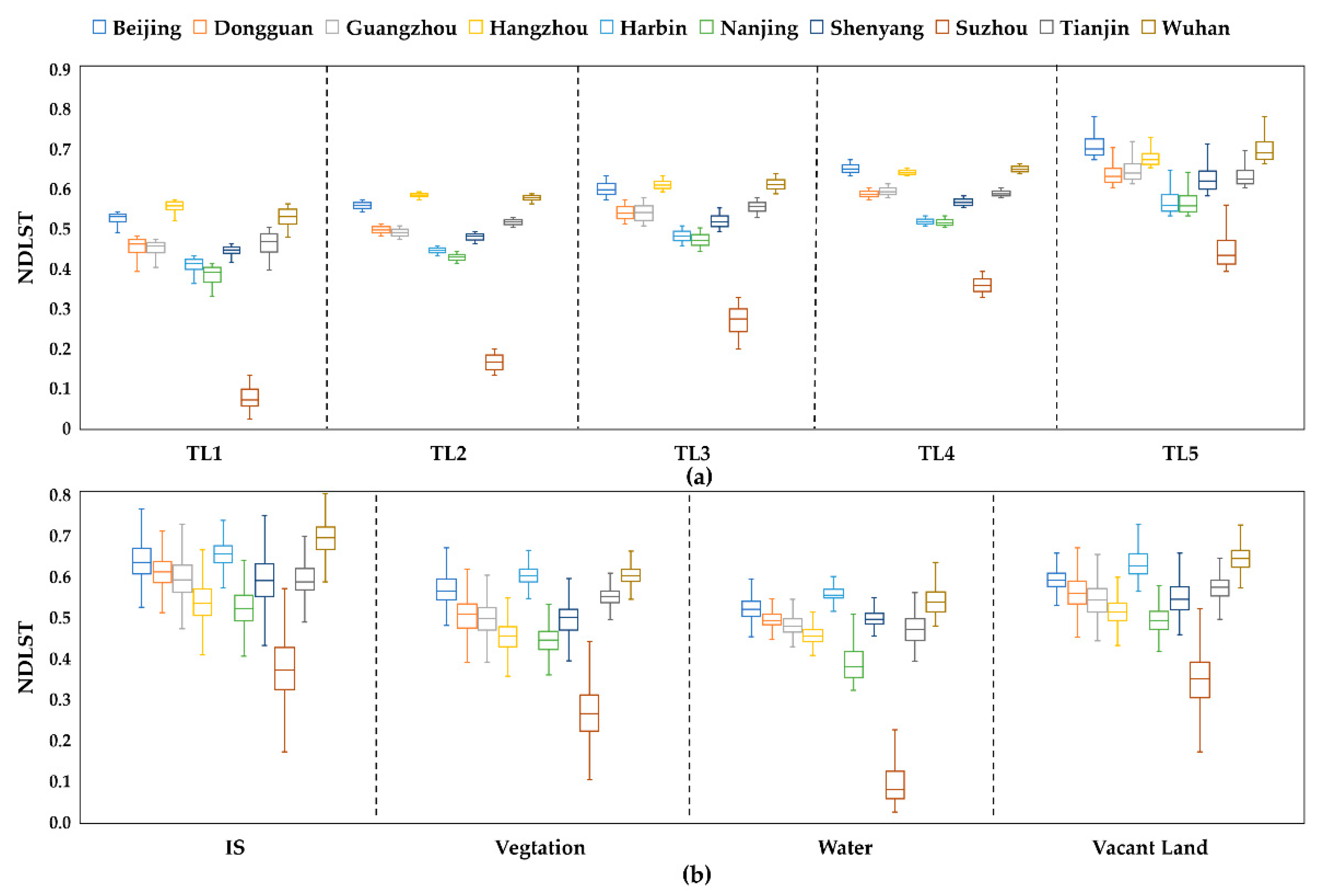
As shown in Figure 4a, we simultaneously compared all cities’ NDLST values for five temperature levels with box-and-whisker plots. The extreme values, median markers, and interquartile range of NDLST values are statistics that we collected and graphically manifested, that convey the temperature distribution information for each class. The majority of mean NDLST values come near the median value, which implies that the distribution of NDLST values is basically not affected by extreme values. As a whole, the boxes for the TL2, TL3, and TL4 zones occupy a narrow range of NDLST values and are symmetrically distributed, indicating that the temperature data from TL2, TL3, and TL4 zones are concentrated and very close to their mean values. However, the TL5 and TL1 zones contain information about the highest and lowest temperatures for each city, respectively. Their box shapes and whiskers represent broader temperature ranges and more significant variability.
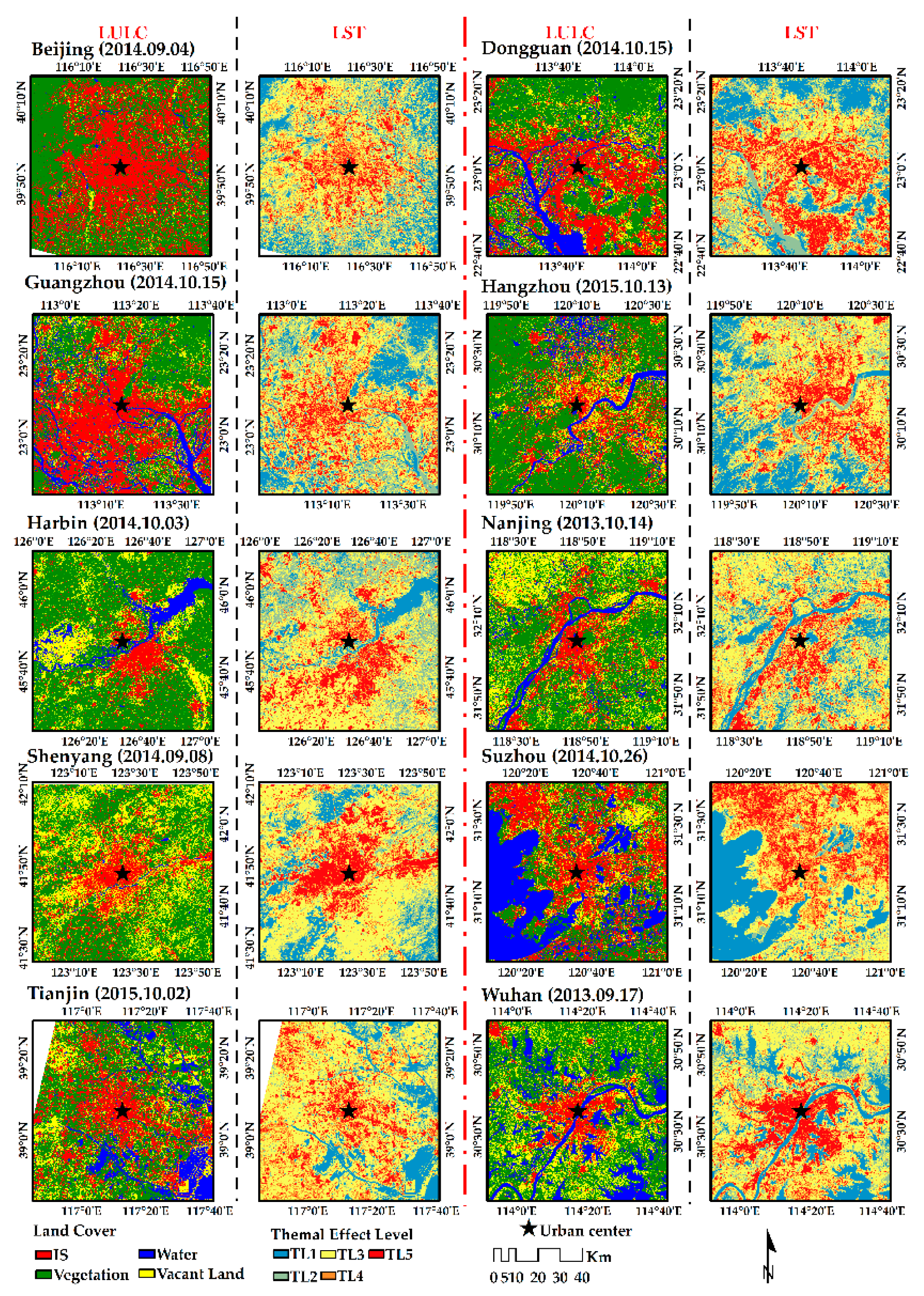
The well-characterized spatial composition and distribution of land cover help enormously to interpret the properties and patterns of the thermal environment. The LULC and LST thematic maps (Figure 3) indicate that the ten megacities have considerable high-urbanized magnitudes, with different spatial arrangements and thermal layouts. However, as shown in Figure 3, the spatial distribution of the thermal environment in the ten megacities is deeply aligned with their particular land cover configurations. These Chinese metropolises exhibit a typical urban-rural gradient pattern at a spatial scale, with urban expansion or IS sprawling outward from the downtown to dispersed suburban cores and peripheries, connected by a network of crisscrossing traffic infrastructure.
The spatial pattern of the most prominent concentric zone in each city is shaped in part by the powerful magnetism attached to the central business district (CBD) and the expansion of ring roads. Beijing famously possesses a highly urbanized ring layout between Tiananmen Square (the CBD) and its neighborhood. Guangzhou and Dongguan stand out with apparent sector configurations in the urban agglomeration of the Pearl River Delta. The Yangtze River runs through the metropolises of Wuhan and Nanjing, which have a complex, decentralized, multi-nuclear pattern. Shenyang and Harbin have a constellation-type pattern due to the strong magnetism of the inner city and multiple scattered suburban cores. Tianjin, Hangzhou, and Suzhou contain intricate clusters and radial patterns owing to their terrain.
The composition and arrangement of land surface cover profoundly affect the attributes and patterns of the thermal environment, as shown in Figure 3. The overall response of thermal layout in each city is in line with the spatial composition of land cover. Generally, the higher temperature zones are concentrated in the center, rapidly diffusing to outskirts with lower temperatures, in a pie shape. The TL5–TL4 zones in Beijing and Tianjin are distinctly located in the inner city. Guangzhou and Dongguan’s TL5–TL4 zones are clustered along the coastline of the delta because of terrain constraints. The primary TL5–TL4 zones of Wuhan and Nanjing are separated by the Yangtze River. The higher-temperature zones in Hangzhou, Shenyang, and Harbin are complicatedly distributed and separated by rivers as well, with scattered high-temperature cores in the suburbs. Suzhou’s thermal layout is significantly influenced by water.
Next, we observed temperature distributions in relation to land cover using boxplots (Figure 4b). On the whole, surface temperature distribution and patterns of land cover in the ten megacities are similar. As shown in Figure 4, the highest temperature always falls under the category of IS, whereas vegetation and/or water are also manifest, consistent with the comparative analysis based on the mean NDLST values of each type of land cover. The temperatures of non-IS surfaces are more intense and closer to the mean NDLST values than those of ISs. However, Suzhou’s temperature pattern is more distinctive than those of the other cities because of the large proportion of water and internal heterogeneity of the land surface.
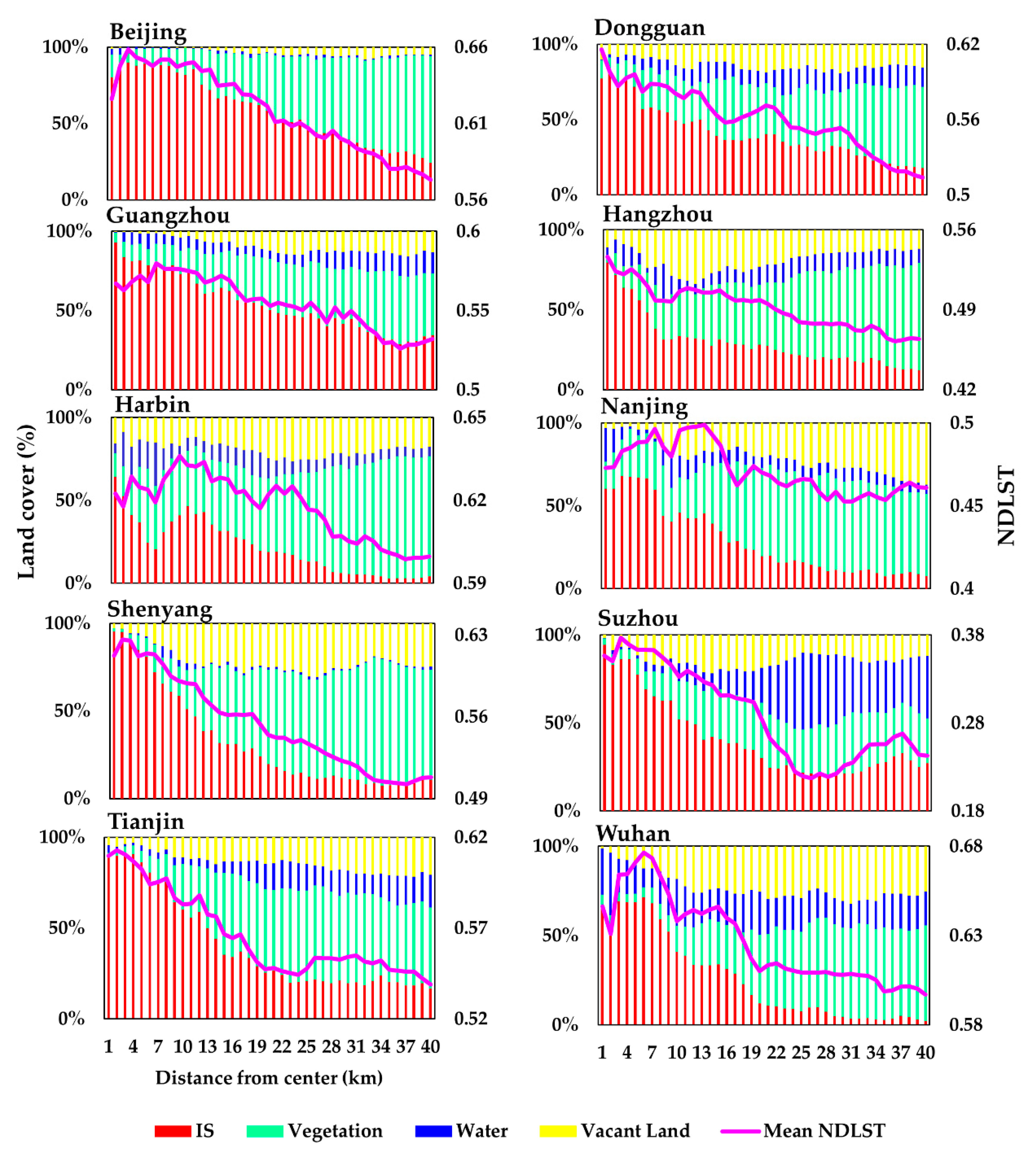
Based on the conceptual model of SUHI, we identified SUHI magnitude across the megacities using the urban-rural gradient model and compared its extent in each city using MURI. Forty concentric zones emerged in each study region, with the urban center as the origin and 1 km intervals between zones. We computed and profiled the composition proportions of land surface cover and the mean NDLST values based on each concentric zone. The results from the SUHI assessments show that the patterns of the mean NDLST values are generally identical to the tendency of ISs and are significantly impacted by non-ISs (Figure 5). The mean NDLST values increase because of the accumulation of ISs and bare soil, whereas the substantial growths of green space and water mitigates the heat effect. Although the overall thermal pattern diffuses from the city core to the surrounding rural areas, the peak values of surface temperature are not always distributed in the urban center.
In the Beijing Metropolitan Area, the temperature peak value is distributed within 3 km from the urban core and the NDLST values contain several minor fluctuations and overall, decline outside the 3 km zone. The surface temperature of Dongguan generally slips from downtown to the suburban periphery, accompanied by small waves. Analogously, Guangzhou witnesses some small temperature fluctuations. In Hangzhou, the temperature decreases as we move outward, with a temperature valley ranging between zones of 7 and 9 km. Harbin’s temperature pattern is complicated, with high/low temperature alternation. For the surface temperature in Nanjing, we found that the mean NDLST values first arise in the 7 km zone due to large amounts of water and vegetation downtown. The peak temperature is seen in the 9 km zone, and the lowest temperature in the 13 km zone. The surface temperature gradually declines from the 2 km zone to the rural part of Shenyang. Because of the nearby body of water, a large temperature trough emerges between 23 and 33 km in Suzhou. Concerning Tianjin’s surface temperature, a distance of 2 km from the center showed the highest value, and zones of 19 to 25 km existed in the cool valley. In Wuhan, we examined higher temperature values in the range of 3 to 19 km. Therefore, a close relationship between LCC and LST is apparent, as shown in Figure 5. We found that higher temperatures or hot spot zones tend to be considerably concentrated in intense-IS areas involving a densely populated region as well as a location for large-scale anthropogenic activities. Conversely, greenbelts and water corridors help to ease the adverse effects of SUHI.
Previous studies on UHI analysis have generally used UHI intensity to detect temperature difference using the mean value of urban pixels minus that of rural pixels, as derived from satellite infrared thermal imageries [2,67]. Accordingly, in this study, an analysis comparing SUHI footprint across the megacities was carried out by aggregating the UHI conceptual theory and MURI. Urban pixels are generally dominated by IS pixels, whereas non-IS ones are mainly rural pixels. Hence, we also characterized SUHII using the difference between the mean NDLST values of IS and those of non-IS pixels. In Table 3 and Table 4, and Figure 6, we have summarized the statistics of MURI and the differences in mean NDLST values between IS and non-IS, which can help us examine the role of land cover in the thermal environment and compare the magnitude of the thermal effect across the megacities. We discovered that the TL4 zones covered between 10.83% and 19.53% of each study region, and Shenyang had the minimum value, while Suzhou obtained the maximum. The TL5 zones occupy between 10.09% and 20.02% of each study area, and the minimum and maximum value are from Beijing and Dongguan, respectively. Subsequently, we calculated the MURI of ten megacities, which we present here by magnitude of SUHI in ascending order: Beijing (21.26%), Nanjing (21.48%), Harbin (22.80%), Hangzhou (23.12%), Tianjin (23.87%), Shenyang (24.04%), Wuhan (25.17%), Guangzhou (25.43%), Dongguan (29.71%), and Suzhou (31.14%).
We also ranked the temperature difference between IS and non-IS () in each city: Harbin (0.0453), Tianjin (0.0523), Nanjing (0.0681), Beijing (0.0711), Shenyang (0.0741), Hangzhou (0.0765), Wuhan (0.0921), Guangzhou (0.0937), Dongguan (0.1003), and Suzhou (0.1620). However, the maximum differences between IS and vegetation or vacant land are both from Dongguan ( 0.1171; 0.0537, respectively), and the maximum value of is in Suzhou (0.2783). In contrast, we obtained the minimum values of from Tianjin (0.0437), Hangzhou (0.0842), and Harbin (0.0186), respectively. This implies that various kinds of LCC play diverse roles in different thermal environments.
Noteworthily, these differences of mean NDLST values for all megacities were verified using the non-parametric Wilcoxon–Mann–Whitney (WMW) rank-sum test. The utilization of the WMW test is to examine the possible differences in the locations of two group means, for which the null-hypothesis is that the two groups of mean NDLST differences come from the same distribution (to test for < 0.05) [78]. Besides, the parametric two-sample t-test method [78] was also applied to check the differences of mean NDLST values between IS and non-IS categories. The t-test statistical analysis was performed based on one-tailed unequal variances. These means can be confirmed whether they are statistically significantly different across megacities. On the ground of these two statistical tests, it can be able to identify three hypotheses about Table 4: (1) the mean NDLST values of the IS category were higher than these of non-IS categories, which reflect the higher temperature in the urban areas and the existence of UHI phenomenon in all megacities. (2) Vegetation plays an outsize role in the non-IS categories, for which the means calculated from the and are not statistically different across megacities. (3) The pixels of water and vacant land have different influences on different megacities, and their means from and compared to those of are statistically significantly different.
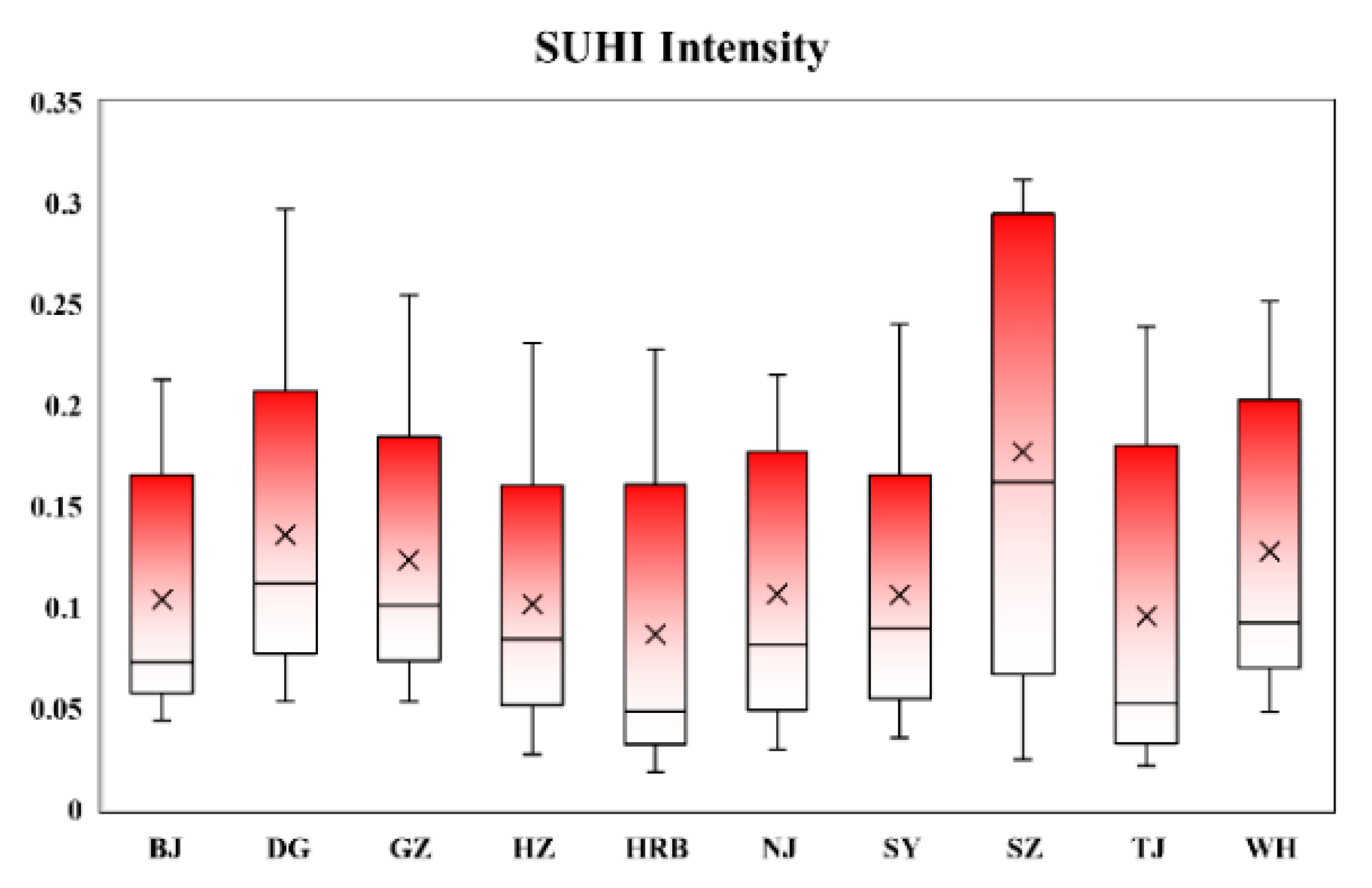
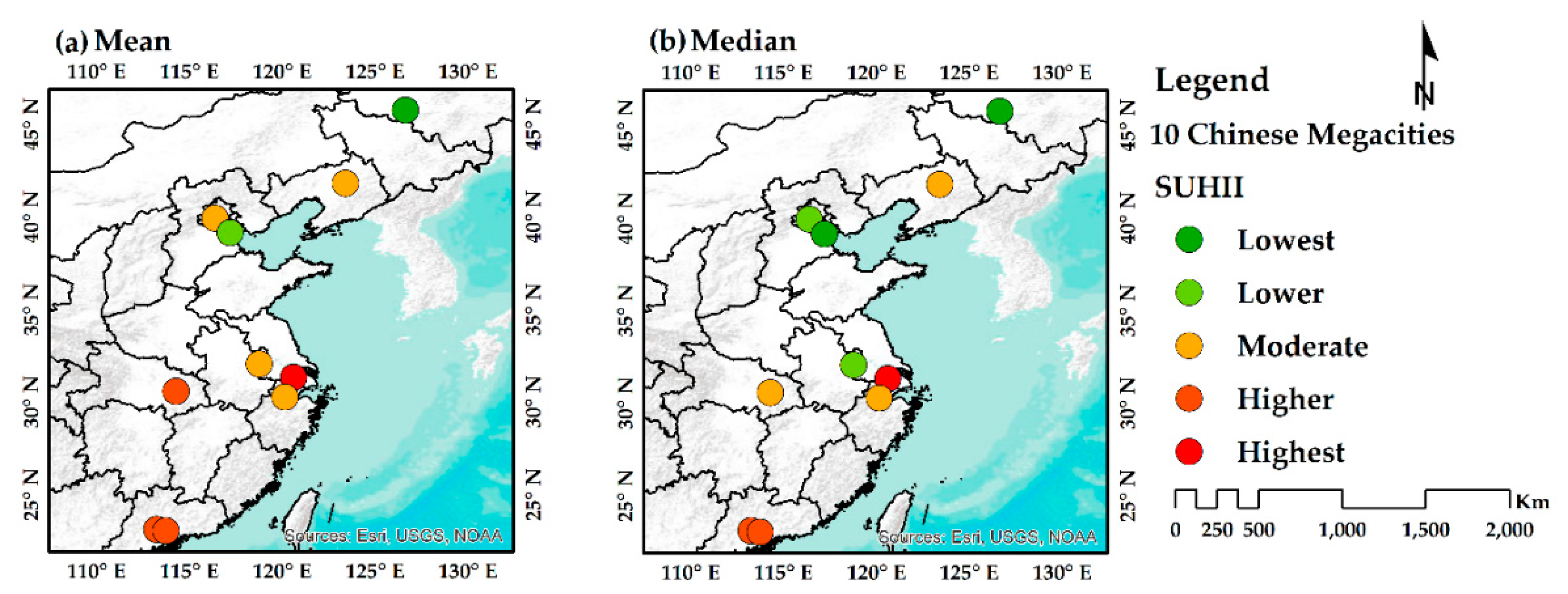
The SUHI footprint varies substantially under different methods. The mean NDLST values of land cover and MURI for all megacities are plotted in Figure 6. We categorized all megacities into five groups using the Jenks Natural Breaks Optimization method [79], representing each SUHI index from lowest to highest. Among varying SUHI footprints, Dongguan, Guangzhou, and Suzhou always presented an intense UHI, whereas the UHI effects in Harbin and Shenyang were relatively lower than those of other megacities. We graphed the different SUHII estimates with box-and-whisker plots to avoid bias regarding SUHII (Figure 7). According to the interquartile range, as well as the median and mean values of the boxplots, Suzhou has the strongest SUHI, while Harbin’s SUHI is weaker than in other cities. Figure 8 presents the SUHI footprint for all megacities, summarized and visualized on the basis of the mean and median values.
3.2. Diagnostics of OLS and GWR
As shown in Table 5, the two explanatory variables—NMPD and LCC%—explained 6.7–28.1% of SUHI formation in the ten megacities according to the estimated R-squared of the OLS regression model. Referring to the estimated coefficients of determination in OLS regression models, we found that the LCC% in the ten megacities is negatively correlated with the average SUHII. As expected, the NMPD varies positively with the average SUHII. Additionally, the t statistics of NDMP and LCC% coefficients for all megacities indicated the statistically significant ( < 0.01) relationships between the SUHII and all explanatory variables. The SUHII of all targeted megacities present the same patterns in terms of LCC and population impacts. However, these lower R2s signify that the conventional OLS global regression model cannot satisfy our needs; by contrast, the outputs of the GWR local-based spatial model may be more trustworthy and reliable in terms of capturing the association among SUHII, population, and LCC. Although the performances of LCC% and NMPD are not so good (R2 < 0.4) in the global regression analysis of SUHI formation, these two explanatory variables are outperformed (R2 > 0.6) in identifying the driving force of SUHI formation at a local scale. As shown in Table 5, the NMPD and LCC% in all study megacities indicate a good fit with R2 > 68.2%, which means these two explanatory variables explain more than 60% of SUHI formation in each megacity, based on the GWR model. Especially in Dongguan, Shenyang, and Suzhou, 80% of SUHII can be illustrated by LCC and population using local regression analysis. The highest estimates of the NMPD coefficient in Suzhou based on global analysis implied that the impact of population on the thermal environment was stronger for Suzhou than for the other targeted megacities, while population affected Tianjin’s thermal environment the least among the ten megacities. Similarly, the layouts of land cover types in Guangzhou had a significant influence on its UHI, according to the local absolute coefficients of LCC%.
However, it is noteworthy that the local impact (local factor) of LCC% and NMPD might vary spatially in different ways by location. Thus, the population positively influenced SUHI formation, where human settlements were also crucial to the urban thermal field, and thereby, anthropogenic heat has a significant effect on the thermal environment and raises the occurrence of UHI. In addition, for all study regions, the presence of spatial non-stationarity was detected on the standardized residuals from both OLS and GWR models using the spatial autocorrelation (i.e., Global Moran’s I Index) tool. Also, these standardized residuals spatially exhibited a clustering distribution. However, the effects of spatial clusters generated by the OLS global model were in more apparent contrast with these generated by GWR. These findings state that it is possible to interpret most of the spatial patterns of SUHI magnitude, as well as the statistically significant relationships in these ten megacities, using the explanatory variables of LCC and population based on the GWR model. In brief, for all targeted megacities, the GWR models seem suitable for exploring and modeling the linkages among SUHII, LCC, and PD that exhibit spatial non-stationarity.
4. Discussion
4.1. Responses of Land Cover to UHI: The Similarities and Differences Among Cities
As mentioned previously, we profiled the proportion of land cover and temperature variations by contrasting urban and rural circumstances. Using Landsat data, we spatially identified SUHII associated with the land cover layout to assess the extent and magnitude of intense SUHI. Herein, we examined the linkages between surface temperature distribution and each land cover type. IS and vacant land (such as bare soil and land) dominate the TL5 and TL4 zones, whereas vegetation and bodies of water serve as essential components for the TL1 and TL2 zones. Notably, massive, dried vegetation and croplands have played a crucial role in higher-temperature areas, which always act as heat sources to promote SUHI. The heat contribution graphics for Harbin, Shenyang, Nanjing, and Dongguan provide the evidence (Figure 9), and other previous studies on UHI have also mentioned this [75,80].
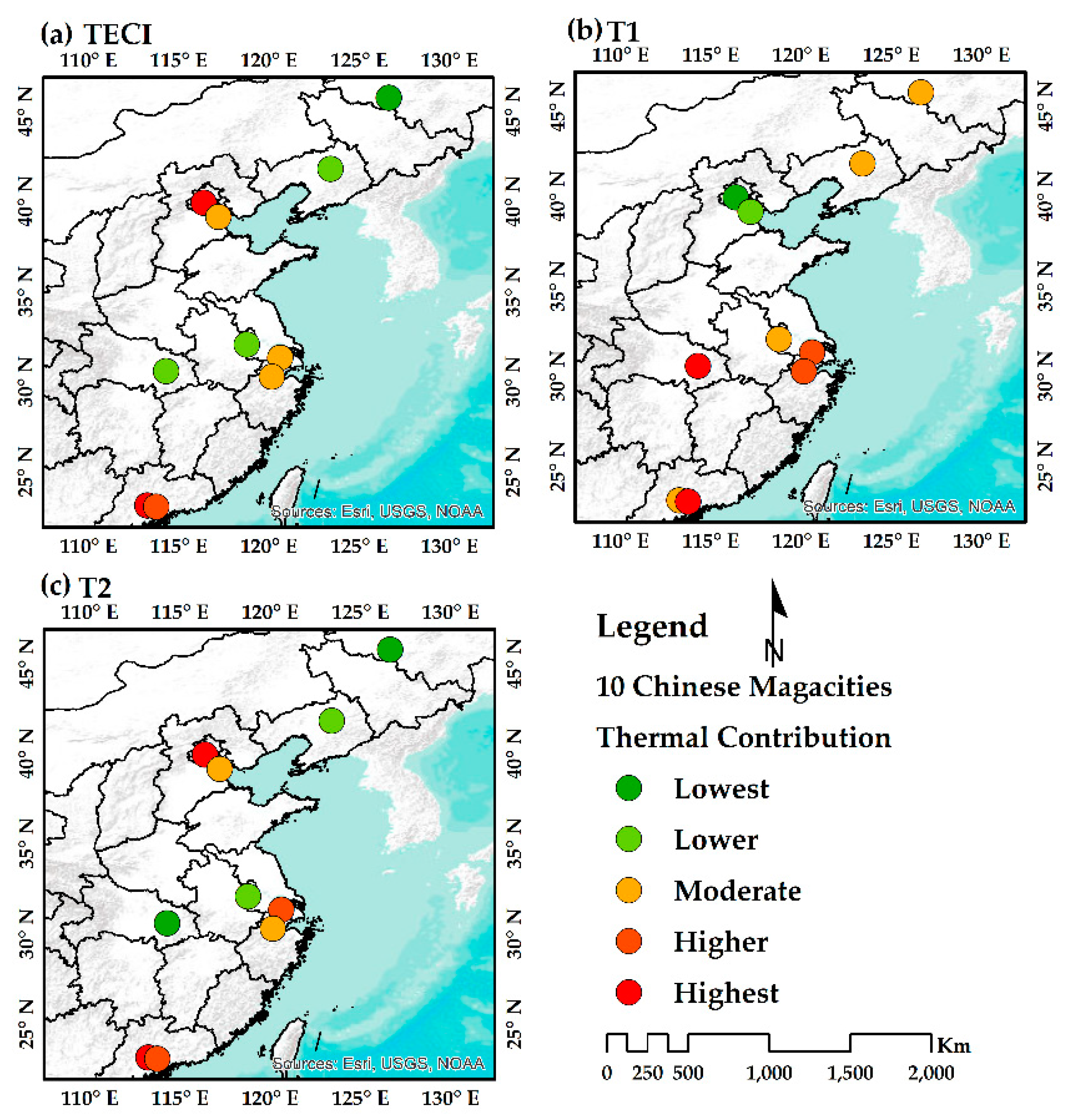
Because of local atmospheric properties, it is meaningless and inaccurate to directly compare the estimated LST values of different cities. In this study, we instead used three urban thermal environment indices (TECI, T1, and T2) to compare the effects of land surface cover on the thermal environment in multiple cities. From the angle of TECI, on the whole, we observed that IS and vacant land (such as bare land) accounted for the prevailing thermal source (39.1% < IS’s TECI < 87.6%; 2.5% < vacant land’s TECI < 43.2%). Vegetation (mainly cropland) also contributed considerably to the heat effect (3.6% < vegetation’s TECI < 26.6%). Nevertheless, water generates less heat budget for the thermal environment (water’s TECI < 1.5%), and different types of land cover possess unique thermal properties. On this basis, we can infer that IS occupies a dominant share of pixels, with above-average NDLST values for all the megacities. Analogously, pixels of bare land also account for a higher percentage; however, green space (except for cropland and dried vegetation) and water have relatively lower shares, in which the NDLST values of fewer pixels are higher than the mean NDLST values. In Beijing and Guangzhou, over 85% of the above-average NDLST pixels belong to IS, while 39.1% of above-average NDLST pixels in Harbin are also IS pixels and most contributed to heat. The TECI values of water in all the megacities are less than 1%, which means that water should be incapable of being a major heat source.
T1 reveals the proportion of above-average NDLST values for a specific kind of land cover, whereas T2 indicates the corresponding specific land cover percentage of above-average NDLST values, accounting for the entire study region. IS exhibits extremely high T1 values for each megacity. This suggests that almost all—or the majority of—IS materials are thermal source materials because of their high heat flux and capacity. Vacant lands also show high T1 values, which implies that bare land also makes a significant thermal contribution across study regions. For vegetation, there are various influences on different thermal regions based on multiple T1 values due to the contribution of cropland heat flux; however, water presents lower T1 values than the other land cover types in the different regions, which means that water has a negative influence on the initiation of the thermal effect.
Different types of land cover exhibit unique functions and behaviors in each megacity. T2 reflects the extent of SUHI resulting from different land cover behaviors across the entire regional scale. Because of the consideration of all land cover proportions, the IS does not present a very high T2 value compared to the TECI and T1 values. In some study regions, entire land surfaces were accounted for by vast expanses of bare land and cropland, resulting in higher T2 values in terms of vegetation and vacant land that are associated with higher heat flux through bare or semi-bare surfaces. Examples include, Hangzhou, Harbin, Shenyang, Nanjing, Tianjin, and Wuhan. Water still makes a minor contribution to the entire regional thermal effect.
By combining the urban-rural gradient analysis and the outcomes of thermal contributions, we can confirm that it is IS that primarily drives the phenological effects of the urban thermal environment. Hence, we further investigated the relationship between LULC and SUHI based on the proportion of IS and the corresponding thermal environment index for different study regions. Figure 10 ranks the thermal contribution index (TECI, T1, and T2) of ISs for all megacities The TECIs of ISs for each megacity are listed with a descending order: Guangzhou (87.56%), Beijing (85.64%), Dongguan (78.86%), Suzhou (62.61%), Tianjin (57.24%), Hangzhou (56.02%), Shenyang (46.57%), Wuhan (43.21%), Nanjing (43.19%), and Harbin (34.21%). The T1 values of IS for each study region are close and intense: Wuhan (97.63%), Dongguan (96.64%), Suzhou (95.05%), Hangzhou (93.15%), Harbin (90.76%), Guangzhou (89.90%), Nanjing (89.50%), Shenyang (88.77%), Tianjin (86.69%), and Beijing (81.01%). The T2 values of IS for each megacity are also shown in descending order: Guangzhou (35.07%), Beijing (33.30%), Dongguan (28.05%), Suzhou (27.91%), Tianjin (20.99%), Hangzhou (17.81%), Nanjing (14.30%), Shenyang (13.71%), Wuhan (10.61%), and Harbin (10.26%). These indexes may significantly reflect the magnitude of SUHI based on the land cover models for different megacities. Furthermore, the rate of IS is strongly related to the corresponding TECI index for cities, with a high coefficient (R2 = 0.9219). In addition, the IS share of each study region is substantially associated with its T2 index, with a high determination coefficient (R2 = 0.9768). However, the proportion of IS for cities is negatively correlated to the relevant T1 index value, with a very low determination coefficient (R2 = 0.1713) (Figure 11). This outcome likely results from the interior interaction effect of impervious materials or from neighboring environmental influences. Last but not least, the rates of IS, IS thermal contribution, and SUHII across diverse Chinese cities are plotted in Figure 12. The chart symbol is scaled to equal 0.49, which is half the size of the most significant value. A SUHI footprint can be identified across the cities.
The multi-city comparative analysis of SUHI footprint might be a dynamic, flexible, and improvable process. Apparently, in this study, there are both differentiations and convergences in the assessment of multiple thermal environments. Despite the fact that SUHI patterns of different cities were highly localized and the magnitude of SUHI varied based on measurement methods, the inherent physics behind SUHI formation are similar and influenced by multiple drivers. Herein, ten Chinese megacities were merely investigated in this study. However, the more specific interpretations and explorations are ongoing for eliciting the valuable information about the association between SUHI and land cover/use. We expect to extend our study covering more comparable megacities, not only in China but also in other countries, such as Tokyo, London, Paris, Berlin, etc. The impact of SUHI on more megacities could be gauged and compared using remote sensing data, under serious consideration of the local climate context and land surface features.
4.2. Linkages among LCC, Population, and UHI: Thermal Effects in Densely Populated Chinese Megacities
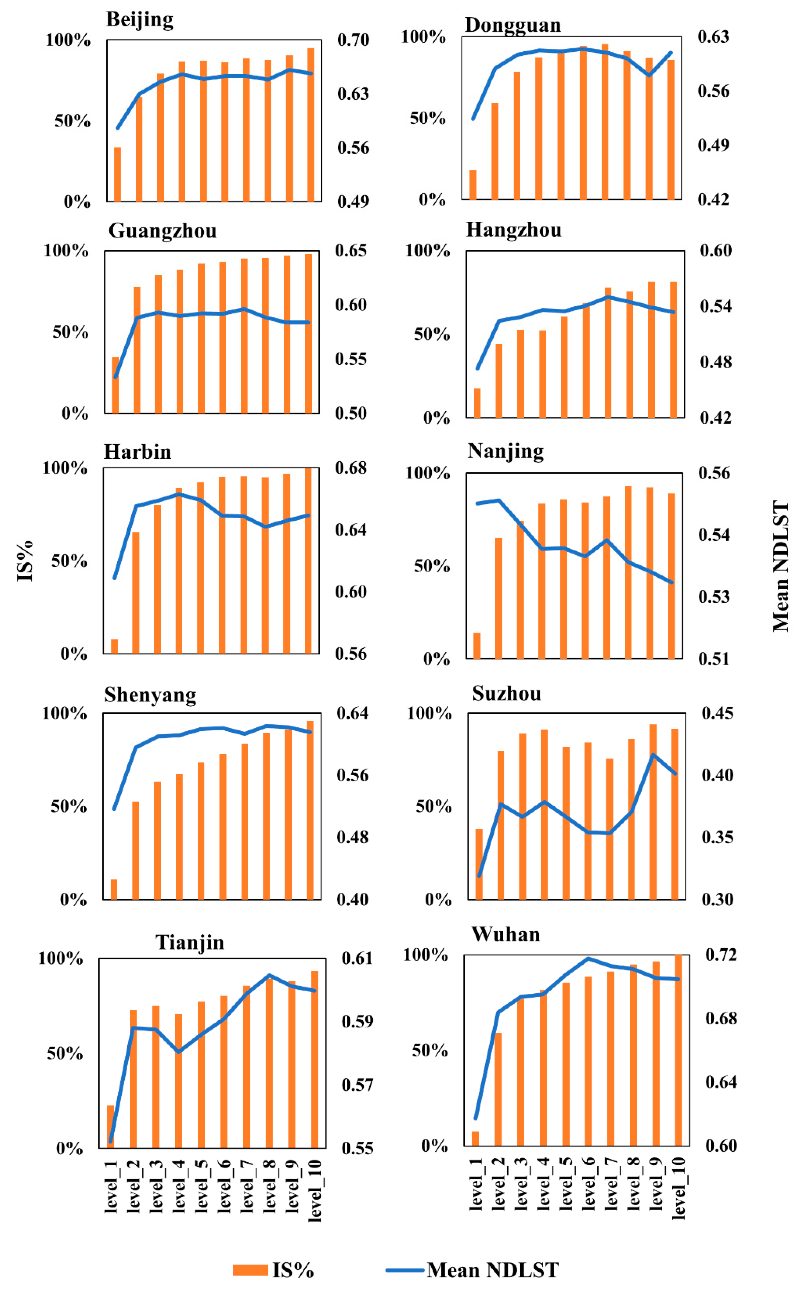
As urbanization accelerates in Chinese cities, urban land demands have a been increasing owing to population gathering and migration. The amount of urban IS has been directly affected, as well as indirectly influenced, by this population. As demonstrated in previous research, the urban environment will be under a certain pressure when the proportion of urban IS in the entire region is 0–10%, will be affected to some extent when the proportion of urban IS in the overall region reaches 10–25%, and will be in severe degradation if the share of urban IS rises above 25% [81]. In brief, severe and diverse consequences could emerge for urban sustainability because of the over-concentration of ISs and population, especially in terms of the urban climate (i.e., the adverse effects of the thermal environment). In this study, we estimated the average proportion of IS for ten cities to be 80.1% of the inner city (within 1 km of the urban center). As indicated earlier, in an ideal situation (standard circumstance), Beijing and Guangzhou possess the largest proportion of ISs and highest heat contribution from ISs in all study regions, with the same size and extent, followed by Dongguan, Suzhou, Tianjin, Hangzhou, Shenyang, Nanjing, Wuhan, and Harbin. SUHII in Harbin is weaker than in other cities. The spatial patterns of the thermal effect in Harbin, Nanjing, Shenyang, and Wuhan are significantly influenced by non-ISs. All megacities are densely populated. To disclose how IS and population influence thermal environment, we divided each megacity into ten levels according to the fraction of PD (0% to 100%, with 10% increments for every level), as shown in Figure 13. We found a non-linear (logarithmic) pattern in each study region between the share of IS and mean NDLST values based on population fraction levels, excluding Nanjing. The IS densities and mean NDLST values gradually expand as PD increases, with small waves providing crests, valleys, plateaus, and basins. However, the mean NDLST values in Nanjing fall slightly from sparsely populated regions to densely populated zones because of a large number of semi-bare and bare areas of land with high temperatures. Such findings might better replenish our interpretation of the associations among SUHI, LCC, and PD.
In tandem with our preliminary analysis and outcomes, we can fulfill the examination of the SUHI–LCC–PD causal mechanism in ten Chinese megacities. To interpret the spatial patterns and the SUHI–LCC–PD relationship in the different study regions, we conducted OLS and GWR analyses to scrutinize the connection between average SUHII values and the explanatory variables (LCC% and NMPD) from both global and local angles. The outputs of the regression analysis showed that both LCC% and NMPD are significant predictors of SUHII. We confirm that these two explanatory variables have an overall consistent influence on thermal environments in the ten megacities. A small increase in LCC% can bring about a decrease in SUHII, while population gathering results in the worsening of SUHI. However, the underlying mechanism of SUHI is also context-sensitive and should be identified over space. The LCC% and NMPD similarly presented locally individual differences based on spatially varying coefficients. These imply that adjusting the ratio of IS to non-IS may help relieve the UHI effect. Furthermore, in the study areas of Suzhou, Shenyang, Dongguan, Hangzhou, and Guangzhou, the impact of LCC% and NMPD variables was more potent for explaining SUHI formation, while the influence of these two variables in Nanjing, Wuhan, and Harbin may not be as substantial as other megacities.
Overall, the preliminary analysis showed that the composition of land cover and the aggregation of the population have significant causal linkages with SUHI formation, irrespective of the local climate context. In other words, it is crucial for an efficient UHI mitigation strategy to decentralize anthropogenic heat by optimizing land use and the allocation of human activities.
4.3. Implications for UHI Mitigation and Further Suggestions for Urban Sustainability
The idea behind this study was to conduct a dynamic multi-city analysis of SUHI in China in spatial context using Landsat archives and then think about how to minimize the UHI effect from the perspective of land cover and population. Chinese megacities share specific characteristics: an excessive rate of IS, an over-dispersed urban green space, and an increasing population, all of which significantly impact their thermal regulation. Before this study, we inferred that there is a causal mechanism among land cover, population, and SUHI in multiple Chinese megacities. The findings proved that our hypothesis was acceptable and reasonable. Thus, by targeting urban sustainability in Chinese megacities, this study suggested that improving the ratio of non-IS area to the IS area (LCC%) and enacting reasonable land settlement and population redistribution policies will contribute to creating SUHI mitigating plan.
First of all, policy makers should focus on the LCC level of the urban environment, which balances and configures urban land use, especially the proportions of IS and greenspace. Based on the thermal contribution of land cover, IS serves as a huge thermal source in each megacity. For the sake of sustainable solutions to relieve UHI, it is unrealistic to remove or demolish large buildings or skyscrapers directly, instead, IS development and urban sprawl in megacities should be scientifically and effectively regulated. Urban surfaces primarily comprise high- and low-albedo IS (including pavement, cement, and concrete). In our study, we derived all surface temperatures from satellite thermal imageries taken in September and October (autumn). In summer and autumn, the urban surface can absorb plenty of solar radiation and store abundant amounts of heat due to the high heat capacity and thermal conductivity of IS. This results in a sharp rise in the surface temperature that subsequently initiates an obvious UHI. However, there are also apparent NDLST valleys in the downtown areas of some megacities, according to our SUHI monitoring outcomes. Except for the influences from adjacent pixels of non-ISs, the IS materials and environment configuration also make substantial contributions. As shown in other studies [3,4,11,82,83], an increasing amount of high-albedo IS materials are currently utilized in building urban infrastructure. For instance, in Adelaide [84], Athens [85], Boston [86] and Guangzhou [11], these megacities have been recommended to optimally cool down the urban temperature and mitigate the UHI effect by adopting the high-albedo building materials. This is a critical step toward alleviating the release of urban heat and facilitating infrastructure construction in low-temperature corridors, because the heat behavior of high-albedo IS causes solar radiation to be reflected rather than absorbed. In the last decade, the inner city—whether redeveloped or rebuilt—has served as the primary agent of urbanization in megacities. Therefore, the construction policy of cooling megacities through high-albedo replacement of low-albedo IS materials in all kinds of facilities (including building roofs, pavement, and transportation networks) could substantially diminish the volume of urban heat emission. However, studies on materials’ thermal properties are usually based on in-situ measurements and are not suitable for retrieving information through thermal remote sensing data. We can further identify it when data become available in the future.
In the context of reasonably regulated IS construction, the arrangement and composition of land cover should not be ignored. Adding green space and bodies of water could neutralize and moderate the thermal effect generated by IS. In the present study, as identified in the results of the GWR model, we found that the increase in LCC% helped decrease surface temperature and alleviate the adverse effects of UHI in megacities. It shows that non-IS land (mainly vegetation) has a significant impact on cooling urban temperature. In the urban-rural gradient analysis of the thermal environment, we also observed that green space and water easily facilitate low-LST corridors, reducing the thermal effect. Therefore, fostering sustainable green cities is a significant part of urban policy in numerous Chinese megacities [13,87]. Previous studies have shown that forests, greenbelts, and water play a decisive role in the thermal regulation of the urban ecological environment [3,88]. The surface temperature drops sharply when green space and water increase on a large scale. The construction of urban green belts or infrastructure, as effective, sustainable solutions for cooling UHI, involve adding green facades, green roofs, vertical gardens, street trees, urban forests, and urban parks [4,26]. Urban heat radiation declines by 2℃ for every 10% increase in urban green space [89]. Furthermore, the ecological environments of cities, such as Suzhou and Wuhan—which are primarily affected by water rather than vegetation—are sensitive to variations in water layout and the construction of blue infrastructure. SUHI mitigating in such megacities with higher proportions of water pixels might vary considerably based on the type, geometry, and proportion of the waterbody. Therefore, blueprints of sustainable urban management should place particular emphasis on the effective arrangement of water (e.g., an increase in urban fountains and pools [90]).
However, the most challenging UHI mitigation strategy is how to accommodate the increase in population in the context of wishing to optimize the spatial layout of urban land use. Urban planning in Chinese cities has placed a great emphasis on human-oriented, sustainable urban development and ecological civilization construction. Site-specific urban policies and regional land use planning are vital to arrange a dense population without deteriorating the rate of IS against non-IS (LCC%). The outputs of the GWR analysis indicated a highly spatial heterogeneity for SUHI in Chinese megacities. Nevertheless, we did not carry out an in-depth analysis of the details of the SUHI formation mechanism in this study. In the future investigation, we expect to carry out several studies such as Li et al. [34], Zhao et al. [32], and Deilami et al. [31], which deeply analyzed a single or a couple of megacities’ SUHI mechanism and variations based on the locally detailed spatial modeling. Such studies might provide specific policies to balance other regional land use imperatives and alleviate local UHI pressure. Moreover, more precise urban metrics information can be expected to be exploited in our future investigation. The characterization of urban typologies and urban forms can benefit the urban design [91,92] for ameliorating the UHI situation. Hence, the answer lies in finding a strategy that suitably regulates IS expansion and layout by considering the urban population and carrying capacity, coordinating the enrichment of green and blue infrastructures.
5. Conclusions
This study addressed the linkages between the UHI effect and geographical process in ten Chinese megacities by examining the spatial configurations of land cover and the influence of population, then translated the key findings into urban management policies. The outcomes provide valuable hints for diminishing UHI and/or enhancing the urban greenspace cooling island (UGCI) effect, and finally suggest a possible path to solve urban climate issues sustainably.
The spatial mapping of land cover and thermal environments indicates that, overall, the thermal gradients of the ten Chinese megacities we examined were radiating outwards from downtown to the periphery. Remarkably, the SUHI footprint fades spatially with distance from the center, which is in line with the urban-rural gradient theory. The trends of NDLST variation closely reflect the spatial composition of land cover: positively correlated with the tendency of IS to change, and negatively influenced by vegetation and water. Although the average proportion of IS for all megacities occupies 80.1% in inner cities, the peak NDLST values are not always located in the urban core. Adding green space and water and using new, high-albedo IS materials all potentially affect the thermal environment. The ecological environment of dense IS distributed throughout the city proper has been improving and developing sustainably.
In our comparative study, we identified the SUHI footprint based on the urban-rural gradient model and MURI, which represent the magnitude and extent of the UHI effect, respectively. According to the degree of SUHI (MURI), Suzhou and Dongguan have a stronger UHI effect than the other megacities. In terms of the magnitude of SUHI (the temperature difference between IS and non-IS), Suzhou ranks the highest, followed by Dongguan, Guangzhou, and Wuhan. In addition, the SUHII estimate in Harbin is always weaker than in the other cities. Based on the mean values of varying SUHII estimates, it can be concluded that SUHII is the most intense in Suzhou. SUHII in Dongguan, Guangzhou, and Wuhan is relatively high. Beijing, Hangzhou, Nanjing, and Shenyang have average SUHII conditions, while it is somewhat low in Tianjin and lowest in Harbin. In addition, SUHII in Suzhou is the most varied because of nearby large bodies of water and vegetation.
High-resolution data from WorldPop greatly help us identify the cities’ thermal environment characteristics. From a holistic angle, the spatial interpretations revealed by the SUHI–LCC–PD causality show that the population is also an essential factor in thermal behavior across diverse cities. Further, the effect of UHI is spatially sensitive to the variations in LCC and population in the local regression modeling, and the GWR model is superior to the conventional global regression model for explaining the causal mechanism of the UHI effect, which can detect locally detailed differences and thus provide valuable insight into the regulation and implementation of regional policy on UHI mitigation.
We examined the spatial configurations of the thermal environment and land cover, identified “temperature cliffs” in urban-rural or different-land-cover surfaces, quantified the urban thermal contributions of land cover, and investigated the impact of population and land cover layout on the thermal effect. Our findings provide significant evidence for addressing the thermal effect and local climate issues, as well as abundant, valuable information to guide urban ecological development policy. In the process of contemporary urban growth, there are urgent needs regarding how to regulate the urban building red line (the proportion of IS), the ecological green line (the scope of green space), and the blue line (the extent of water). Achieving an optimized layout of land cover/use will enable us to take advantage of limited urban space to improve the living environment, slow down the urban thermal effect, adjust to the local climate, and promote the most excellent ecological environment possible.
Author Contributions
Research design, execution, and writeup, F.L.; writeup and revision, X.Z.; topic proposal and comments, Y.M.; review and revision, T.M. All authors have read and agreed to the published version of the manuscript.
Funding
This research was supported by the Japan Society for the Promotion of Science (JSPS) through Grant-in-Aid for Scientific Research (B) 18H00763.
Acknowledgments
The authors highly appreciate the reviewers and the editors for their valuable and constructive comments and suggestions to improve the manuscript.
Conflicts of Interest
The authors declare no conflict of interest.
Appendix A

Table A1.
The accuracy assessment of LULC classification.
| City | Overall Accuracy (%) | Kappa Coefficient | Producer’s Accuracy (%) | Producer’s Accuracy (%) | ||||||
|---|---|---|---|---|---|---|---|---|---|---|
| IS | Vegetation | Water | Vacant Land | IS | Vegetation | Water | Vacant Land | |||
| Beijing | 96 | 0.9467 | 97.94 | 96 | 97.96 | 92.38 | 94.06 | 96 | 96 | 97.98 |
| Dongguan | 93.25 | 0.91 | 85.98 | 97.06 | 98.02 | 92.22 | 92 | 99 | 99 | 83 |
| Guangzhou | 94.5 | 0.9267 | 90.74 | 98 | 95.15 | 94.38 | 96.08 | 98.99 | 98.99 | 84 |
| Hangzhou | 90 | 0.8666 | 80.53 | 95.15 | 96.91 | 88.51 | 91.92 | 94.23 | 94 | 79.38 |
| Harbin | 94.75 | 0.93 | 94.12 | 98.96 | 98.87 | 87.62 | 95.05 | 95 | 96 | 92.93 |
| Nanjing | 90.75 | 0.8766 | 88.89 | 96.59 | 95.15 | 83.64 | 89.8 | 85 | 98 | 90.2 |
| Shenyang | 91.25 | 0.8833 | 90 | 93.75 | 94.12 | 87.25 | 90.91 | 90 | 96 | 88.12 |
| Suzhou | 91.5 | 0.8867 | 87.27 | 95.79 | 87.72 | 97.53 | 96 | 91.92 | 100 | 78.22 |
| Tianjin | 89.5 | 0.86 | 83.65 | 95.92 | 92.33 | 86.32 | 87.88 | 94 | 95 | 81.19 |
| Wuhan | 90.75 | 0.8767 | 84.55 | 92.93 | 91.74 | 95.12 | 93 | 92 | 100 | 78 |
Table A2.
The summary of atmospheric profiles parameter.
| City | Band Average Atmospheric Transmission | Effective Bandpass Upwelling Radiance (W/m2 · sr · μm) | Effective Bandpass Downwelling Radiance (W/m2 · sr · μm) |
|---|---|---|---|
| Beijing | 0.93 | 0.43 | 0.77 |
| Dongguan | 0.74 | 2.02 | 3.27 |
| Guangzhou | 0.74 | 2.02 | 3.27 |
| Hangzhou | 0.91 | 0.68 | 1.18 |
| Harbin | 0.94 | 0.35 | 0.63 |
| Nanjing | 0.78 | 1.88 | 3.03 |
| Shenyang | 0.88 | 0.9 | 1.53 |
| Suzhou | 0.78 | 1.81 | 2.96 |
| Tianjin | 0.91 | 0.67 | 1.17 |
| Wuhan | 0.68 | 2.84 | 4.5 |
Note: The effective bandpass upwelling/ downwelling radiance and band average atmospheric transmission are generated by Atmospheric Correction Parameter Calculator, NASA (https://atmcorr.gsfc.nasa.gov/index.html).
Figure A1.
The spatial distribution of population density for each study region.

References
- United Nations, Department of Economic and Social Affairs, Population Division, (UN DESA). World Population Prospects: The 2015 Revision; UN DESA: New York, NY, USA, 2015. [Google Scholar]
- Oke, T.R. The energetic basis of the urban heat island. Q. J. R. Meteorol. Soc. 1982, 108, 1–24. [Google Scholar] [CrossRef]
- Gago, E.J.; Roldan, J.; Pacheco-Torres, R.; Ordóñez, J. The city and urban heat islands: A review of strategies to mitigate adverse effects. Renew. Sustain. Energy Rev. 2013, 25, 749–758. [Google Scholar] [CrossRef]
- Deilami, K.; Kamruzzaman, M.; Liu, Y. Urban heat island effect: A systematic review of spatio-temporal factors, data, methods, and mitigation measures. Int. J. Appl. Earth Obs. Geoinf. 2018, 67, 30–42. [Google Scholar] [CrossRef]
- United Nations Development Programme (UNDP). Sustainable Urbanization Strategy; UNDP: New York, NY, USA, 2016. [Google Scholar]
- Gupta, J.; Vegelin, C. Sustainable development goals and inclusive development. Int. Environ. Agreem. Polit. Law Econ. 2016, 16, 433–448. [Google Scholar] [CrossRef] [Green Version]
- United Nations (UN).Transforming Our World: The 2030 Agenda for Sustainable Development. General Assembley 70 Session. 2015. Available online: https://sustainabledevelopment.un.org/post2015/transformingourworld (accessed on 27 August 2019).
- National Bureau of Statistics (NBS) of China. Available online: http://www.stats.gov.cn/english/ (accessed on 3 July 2019).
- Kuang, W.; Liu, J.; Zhang, Z.; Lu, D.; Xiang, B. Spatiotemporal dynamics of impervious surface areas across China during the early 21st century. Chin. Sci. Bull. 2013, 58, 1691–1701. [Google Scholar] [CrossRef] [Green Version]
- Liu, J.; Kuang, W.; Zhang, Z.; Xu, X.; Qin, Y.; Ning, J.; Zhou, W.; Zhang, S.; Li, R.; Yan, C.; et al. Spatiotemporal characteristics, patterns and causes of land use changes in China since the late 1980s. J. Geogr. Sci. 2014, 24, 195–210. [Google Scholar] [CrossRef]
- Xiong, Y.; Huang, S.; Chen, F.; Ye, H.; Wang, C.; Zhu, C. The impacts of rapid urbanization on the thermal environment: A remote sensing study of Guangzhou, South China. Remote Sens. 2012, 4, 2033–2056. [Google Scholar] [CrossRef] [Green Version]
- Zhou, D.; Bonafoni, S.; Zhang, L.; Wang, R. Remote sensing of the urban heat island effect in a highly populated urban agglomeration area in East China. Sci. Total Environ. 2018, 628, 415–429. [Google Scholar] [CrossRef]
- Liu, J.; Deng, X. Impacts and mitigation of climate change on Chinese cities. Curr. Opin. Environ. Sustain. 2011, 3, 188–192. [Google Scholar] [CrossRef]
- Peng, J.; Ma, J.; Liu, Q.; Liu, Y.; Hu, Y.; Li, Y.; Yue, Y. Spatial-temporal change of land surface temperature across 285 cities in China: An urban-rural contrast perspective. Sci. Total Environ. 2018, 635, 487–497. [Google Scholar] [CrossRef]
- Wang, J.; Huang, B.; Fu, D.; Atkinson, P.M. Spatiotemporal variation in surface urban heat island intensity and associated determinants across major Chinese cities. Remote Sens. 2015, 7, 3670–3689. [Google Scholar] [CrossRef] [Green Version]
- Yao, R.; Wang, L.; Huang, X.; Niu, Z.; Liu, F.; Wang, Q. Temporal trends of surface urban heat islands and associated determinants in major Chinese cities. Sci. Total Environ. 2017, 609, 742–754. [Google Scholar] [CrossRef] [PubMed]
- Zhou, D.; Zhao, S.; Liu, S.; Zhang, L.; Zhu, C. Surface urban heat island in China’s 32 major cities: Spatial patterns and drivers. Remote Sens. Environ. 2014, 152, 51–61. [Google Scholar] [CrossRef]
- Zhou, D.; Zhao, S.; Zhang, L.; Sun, G.; Liu, Y. The footprint of urban heat island effect in China. Sci. Rep. 2015, 5, 2–12. [Google Scholar] [CrossRef] [PubMed]
- Zhang, J.; Dong, W.; Wu, L.; Wei, J.; Chen, P.; Lee, D. Impact of land use changes on surface warming in China. Adv. Atmos. Sci. 2005, 22, 343–348. [Google Scholar]
- Zhou, D.; Xiao, J.; Bonafoni, S.; Berger, C.; Deilami, K.; Zhou, Y.; Frolking, S.; Yao, R.; Qiao, Z.; Sobrino, J.A. Satellite remote sensing of surface urban heat islands: Progress, challenges, and perspectives. Remote Sens. 2019, 11, 48. [Google Scholar] [CrossRef] [Green Version]
- Huang, Y.; Yuan, M.; Lu, Y. Spatially varying relationships between surface urban heat islands and driving factors across cities in China. Environ. Plan. B Urban Anal. City Sci. 2019, 46, 377–394. [Google Scholar] [CrossRef]
- Li, K.; Chen, Y.; Wang, M.; Gong, A. Spatial-temporal variations of surface urban heat island intensity induced by different definitions of rural extents in China. Sci. Total Environ. 2019, 669, 229–247. [Google Scholar] [CrossRef]
- Tran, D.X.; Pla, F.; Latorre-Carmona, P.; Myint, S.W.; Caetano, M.; Kieu, H.V. Characterizing the relationship between land use land cover change and land surface temperature. ISPRS J. Photogramm. Remote Sens. 2017, 124, 119–132. [Google Scholar] [CrossRef] [Green Version]
- Yao, R.; Wang, L.; Huang, X.; Zhang, W.; Li, J.; Niu, Z. Interannual variations in surface urban heat island intensity and associated drivers in China. J. Environ. Manag. 2018, 222, 86–94. [Google Scholar] [CrossRef]
- Chen, W.; Zhang, Y.; Pengwang, C.; Gao, W. Evaluation of urbanization dynamics and its impacts on surface heat islands: A case study of Beijing, China. Remote Sens. 2017, 9, 453. [Google Scholar] [CrossRef] [Green Version]
- Li, X.; Zhou, W.; Ouyang, Z.; Xu, W.; Zheng, H. Spatial pattern of greenspace affects land surface temperature: Evidence from the heavily urbanized Beijing metropolitan area, China. Landsc. Ecol. 2012, 27, 887–898. [Google Scholar] [CrossRef]
- Xu, D.; Chen, R. Comparison of urban heat island and urban reflection in Nanjing City of China. Sustain. Cities Soc. 2017, 31, 26–36. [Google Scholar] [CrossRef]
- Li, L.; Tan, Y.; Ying, S.; Yu, Z.; Li, Z.; Lan, H. Impact of land cover and population density on land surface temperature: Case study in Wuhan, China. J. Appl. Remote Sens. 2014, 8, 084993. [Google Scholar] [CrossRef]
- Zhang, X.; Estoque, R.C.; Murayama, Y. An urban heat island study in Nanchang City, China based on land surface temperature and social-ecological variables. Sustain. Cities Soc. 2017, 32, 557–568. [Google Scholar] [CrossRef]
- Zhang, H.; Qi, Z.; Ye, X.; Cai, Y.; Ma, W.; Chen, M. Analysis of land use/land cover change, population shift, and their effects on spatiotemporal patterns of urban heat islands in metropolitan Shanghai, China. Appl. Geogr. 2013, 44, 121–133. [Google Scholar] [CrossRef]
- Deilami, K.; Kamruzzaman, M.; Hayes, J.F. Correlation or causality between land cover patterns and the urban heat island effect? Evidence from Brisbane, Australia. Remote Sens. 2016, 8, 716. [Google Scholar] [CrossRef] [Green Version]
- Zhao, C.; Jensen, J.; Weng, Q.; Weaver, R. A geographically weighted regression analysis of the underlying factors related to the surface urban heat island phenomenon. Remote Sens. 2018, 10, 1428. [Google Scholar] [CrossRef] [Green Version]
- Luo, X.; Peng, Y. Scale effects of the relationships between urban heat islands and impact factors based on a geographically-weighted regression model. Remote Sens. 2016, 8, 760. [Google Scholar] [CrossRef] [Green Version]
- Li, W.; Cao, Q.; Lang, K.; Wu, J. Linking potential heat source and sink to urban heat island: Heterogeneous effects of landscape pattern on land surface temperature. Sci. Total Environ. 2017, 586, 457–465. [Google Scholar] [CrossRef]
- Li, F.; Sun, W.; Yang, G.; Weng, Q. Investigating spatiotemporal patterns of surface urban heat islands in the Hangzhou Metropolitan Area, China, 2000–2015. Remote Sens. 2019, 11, 1553. [Google Scholar] [CrossRef] [Green Version]
- Naughton, B.J. The Chinese Economy: Transitions and Growth; MIT Press: Cambridge, MA, USA, 2006. [Google Scholar]
- Zhang, J.; Wu, L. Modulation of the urban heat island by the tourism during the Chinese New Year holiday: A case study in Sanya City, Hainan Province of China. Sci. Bull. 2015, 60, 1543–1546. [Google Scholar] [CrossRef] [Green Version]
- Zhang, X.; Wang, D.; Hao, H.; Zhang, F.; Hu, Y. Effects of land use/cover changes and urban forest configuration on urban heat islands in a loess hilly region: Case study based on Yan’an City, China. Int. J. Environ. Res. Public Health 2017, 14, 840. [Google Scholar] [CrossRef] [Green Version]
- Zhao, X.; Huang, J.; Ye, H.; Wang, K.; Qiu, Q. Spatiotemporal changes of the urban heat island of a coastal city in the context of urbanisation. Int. J. Sustain. Dev. World Ecol. 2010, 17, 311–316. [Google Scholar] [CrossRef]
- The National Development and Reform Comimission (NDRC). China’s National Climate Change Program (June 2007). Available online: http://www.china-un.org/eng/gyzg/t626117.htm (accessed on 20 September 2019).
- Williams, L. China’s Climate Change Policies: Actors and Drivers. Sydney: Lowy Institute for International Policy. 2014. Available online: https://www.lowyinstitute.org/publications/chinas-climate-change-policies-actors-and-drivers (accessed on 20 September 2019).
- Du, H.; Wang, D.; Wang, Y.; Zhao, X.; Qin, F.; Jiang, H.; Cai, Y. Influences of land cover types, meteorological conditions, anthropogenic heat and urban area on surface urban heat island in the Yangtze River Delta Urban Agglomeration. Sci. Total Environ. 2016, 571, 461–470. [Google Scholar] [CrossRef] [PubMed]
- Liu, F.; Murayama, Y. Landsat evaluation of land cover composition and its impacts on urban thermal environment: A case study on the fast-growing Shanghai Metropolitan Area from 2000 to 2015. Geoinfor Geostat Overv. 2018, S3, 2. [Google Scholar]
- Wentz, E.A.; York, A.M.; Alberti, M.; Conrow, L.; Fischer, H.; Inostroza, L.; Jantz, C.; Pickett, S.T.A.; Seto, K.C.; Taubenböck, H. Six fundamental aspects for conceptualizing multidimensional urban form: A spatial mapping perspective. Landsc. Urban Plan. 2018, 179, 55–62. [Google Scholar] [CrossRef]
- Lloyd, C.T.; Sorichetta, A.; Tatem, A.J. High resolution global gridded data for use in population studies. Sci. Data 2017, 4, 170001. [Google Scholar] [CrossRef] [Green Version]
- Stevens, F.R.; Gaughan, A.E.; Linard, C.; Tatem, A.J. Disaggregating census data for population mapping using random forests with remotely-sensed and ancillary data. PLoS ONE 2015, 10, 0107042. [Google Scholar] [CrossRef] [Green Version]
- Tatem, A.J. WorldPop, open data for spatial demography. Sci. Data 2017, 4, 2–5. [Google Scholar] [CrossRef]
- Phiri, D.; Morgenroth, J. Developments in Landsat land cover classification methods: A review. Remote Sens. 2017, 9, 967. [Google Scholar] [CrossRef] [Green Version]
- Lu, D.; Weng, Q. A survey of image classification methods and techniques for improving classification performance. Int. J. Remote Sens. 2007, 28, 823–870. [Google Scholar] [CrossRef]
- Zhou, W.; Qian, Y.; Li, X.; Li, W.; Han, L. Relationships between land cover and the surface urban heat island: Seasonal variability and effects of spatial and thematic resolution of land cover data on predicting land surface temperatures. Landsc. Ecol. 2014, 29, 153–167. [Google Scholar] [CrossRef]
- Laben, C.A.; Brower, B.V. Process for Enhancing the Spatial Resolution of Multispectral Imagery Using Pan-Sharpening. U.S. Patent No. 6,011,875, 4 January 2000. [Google Scholar]
- Yuhendra; Joshapat, T.S.; Hiroaki, K. Performance analyzing of high resolution pan-sharpening techniques: Increasing image quality for classification using supervised kernel support vector machine. Res. J. Inf. Technol. 2011, 3, 12–23. [Google Scholar]
- Anderson, J.R. A Land Use and Land Cover Classification System for Use with Remote Sensor Data; US Government Printing Office: Washington, DC, USA, 1976; Volume 964.
- Janssen, L.L.F.; van der Wel, F.J.M. Accuracy assessment of satellite derived land-cover data: A review. Photogramm. Eng. Remote Sens. 1994, 60, 419–426. [Google Scholar]
- Galve, J.M.; Sánchez, J.M.; Coll, C.; Villodre, J. A new single-band pixel-by-pixel atmospheric correction method to improve the accuracy in remote sensing estimates of LST. application to Landsat 7-ETM+. Remote Sens. 2018, 10, 826. [Google Scholar] [CrossRef] [Green Version]
- Jin, M.S.; Kessomkiat, W.; Pereira, G. Satellite-observed urbanization characters in Shanghai, China: Aerosols, urban heat island effect, and land-atmosphere interactions. Remote Sens. 2011, 3, 83–99. [Google Scholar] [CrossRef] [Green Version]
- Liang, S.; Fang, H.; Chen, M. Atmospheric correction of Landsat ETM+ land surface imagery—Part I: Methods. IEEE Trans. Geosci. Remote Sens. 2001, 39, 2490–2498. [Google Scholar] [CrossRef]
- McCarville, D.; Buenemann, M.; Bleiweiss, M.; Barsi, J. Atmospheric correction of Landsat thermal infrared data: A calculator based on North American Regional Reanalysis (NARR) data. In Proceedings of the American Society for Photogrammetry and Remote Sensing Conference, Milwaukee, WI, USA, 1–5 May 2011; Volume 15. [Google Scholar]
- Tardy, B.; Rivalland, V.; Huc, M.; Hagolle, O.; Marcq, S.; Boulet, G. A software tool for atmospheric correction and surface temperature estimation of Landsat infrared thermal data. Remote Sens. 2016, 8, 696. [Google Scholar] [CrossRef] [Green Version]
- Barsi, J.A.; Schott, J.R.; Palluconi, F.D.; Hook, S.J. Validation of a web-based atmospheric correction tool for single thermal band instruments. Earth Obs. Syst. X 2005, 5882, 58820E. [Google Scholar]
- Barsi, A.J.; Barker, L.J.; Schott, R.J. An atmospheric correction parameter calculator for a single thermal band earth-sensing instrument. In Proceedings of the 2003 IEEE International Geoscience and Remote Sensing Symposium (IEEE Cat. No. 03CH37477), IGARSS, Toulouse, France, 21–25 July 2003; Volume 5, pp. 3014–3016. [Google Scholar]
- Chen, L.; Jiang, R.; Xiang, W.N. Surface heat island in Shanghai and its relationship with urban development from 1989 to 2013. Adv. Meteorol. 2016, 2016, 9782686. [Google Scholar] [CrossRef]
- Li, Z.; Duan, S.; Tang, B.; Wu, H.; Ren, H.; Yan, G.; Tang, R.; Leng, P. Review of methods for land surface temperature derived from thermal infrared remotely sensed data. J. Remote Sens. 2016, 20, 899–920. (In Chinese) [Google Scholar]
- Shi, T.; Huang, Y.; Wang, H.; Shi, C.E.; Yang, Y.J. Influence of urbanization on the thermal environment of meteorological station: Satellite-observed evidence. Adv. Clim. Chang. Res. 2015, 6, 7–15. [Google Scholar] [CrossRef]
- Ahn, S.; Fessler, J.A. Standard Errors of Mean, Variance, and Standard Deviation Estimators. EECS Dep. Univ. Mich. 2003. Available online: https://web.eecs.umich.edu/~fessler/papers/lists/files/tr/stderr.pdf (accessed on 10 October 2019).
- Sun, Q.; Tan, J.; Xu, Y. An ERDAS image processing method for retrieving LST and describing urban heat evolution: A case study in the Pearl River Delta Region in South China. Environ. Earth Sci. 2009, 59, 1047–1055. [Google Scholar] [CrossRef]
- Estoque, R.C.; Murayama, Y. Intensity and spatial pattern of urban land changes in the megacities of Southeast Asia. Land Use Policy 2015, 48, 213–222. [Google Scholar] [CrossRef]
- Dissanayake, D.M.S.L.B.; Morimoto, T.; Murayama, Y.; Ranagalage, M. Impact of landscape structure on the variation of land surface temperature in Sub-Saharan Region: A case study of Addis Ababa using Landsat Data (1986–2016). Sustainability 2019, 11, 2257. [Google Scholar] [CrossRef] [Green Version]
- Dissanayake, D.; Morimoto, T.; Murayama, Y.; Ranagalage, M.; Handayani, H.H. Impact of urban surface characteristics and socio-economic variables on the spatial variation of land surface temperature in Lagos City, Nigeria. Sustainability 2018, 11, 25. [Google Scholar] [CrossRef] [Green Version]
- De Faria Peres, L.; de Lucena, A.J.; Rotunno Filho, O.C.; de Almeida França, J.R. The urban heat island in Rio de Janeiro, Brazil, in the last 30 years using remote sensing data. Int. J. Appl. Earth Obs. Geoinf. 2018, 64, 104–116. [Google Scholar] [CrossRef]
- Xu, H.Q.; Chen, B.Q. Remote sensing of the urban heat island and its changes in Xiamen City of SE China. J. Environ. Sci. 2004, 16, 276–281. [Google Scholar]
- Xiao, H.; Kopecká, M.; Guo, S.; Guan, Y.; Cai, D.; Zhang, C.; Zhang, X.; Yao, W. Responses of urban land surface temperature on land cover: A comparative study of Vienna and Madrid. Sustainability 2018, 10, 260. [Google Scholar] [CrossRef] [Green Version]
- Simwanda, M.; Ranagalage, M.; Estoque, R.C.; Murayama, Y. Spatial analysis of surface urban heat islands in four rapidly growing African cities. Remote Sens. 2019, 11, 1645. [Google Scholar] [CrossRef] [Green Version]
- Liu, Y.; Kuang, Y.; Wu, Z. Impact of land use on urban land surface temperature: A case study of Dongguan, Guangdong Province. Sci. Geogr. Sin. 2006, 26, 597. (In Chinese) [Google Scholar]
- Lu, D.; Song, K.; Zang, S.; Jia, M.; Du, J.; Ren, C. The effect of urban expansion on urban surface temperature in Shenyang, China: An analysis with Landsat imagery. Environ. Model. Assess. 2015, 20, 197–210. [Google Scholar] [CrossRef]
- Qian, L.; Ding, S. Pearl River Delta land cover change on surface temperature effects. Acta Geogr. Sin. 2005, 60, 761–770. (In Chinese) [Google Scholar]
- Weng, Q.; Lu, D. A sub-pixel analysis of urbanization effect on land surface temperature and its interplay with impervious surface and vegetation coverage in Indianapolis, United States. Int. J. Appl. Earth Obs. Geoinf. 2008, 10, 68–83. [Google Scholar] [CrossRef]
- Wilks, D.S. Statistical Methods in the Atmospheric Sciences; Academic Press: Cambridge, MA, USA, 2011; Volume 100. [Google Scholar]
- Jenks, G.F. The data model concept in statistical mapping. Int. Yearb. Cartogr. 1967, 7, 186–190. [Google Scholar]
- Tursilowati, L.; Tetuko, J.; Sumantyo, S.; Kuze, H.; Adiningsih, E.S. Relationship between urban heat island phenomenon and land use/land cover changes in Jakarta—Indonesia. J. Emerg. Trends Eng. Appl. Sci. 2012, 3, 645–653. [Google Scholar]
- Elvidge, C.D.; Safran, J.; Tuttle, B.; Sutton, P.; Cinzano, P.; Pettit, D.; Arvesen, J.; Small, C. Potential for global mapping of development via a nightsat mission. GeoJournal 2007, 69, 45–53. [Google Scholar] [CrossRef]
- Mohajerani, A.; Bakaric, J.; Jeffrey-Bailey, T. The urban heat island effect, its causes, and mitigation, with reference to the thermal properties of asphalt concrete. J. Environ. Manag. 2017, 197, 522–538. [Google Scholar] [CrossRef]
- Taha, H.; Sailor, D.; Municipal, S. High-Albedo Materials for Reducing Building Cooling Energy Use; U.S. Department of Energy: Washington, DC, USA, 1992.
- Razzaghmanesh, M.; Beecham, S.; Salemi, T. The role of green roofs in mitigating Urban Heat Island effects in the metropolitan area of Adelaide, South Australia. Urban For. Urban Green. 2016, 15, 89–102. [Google Scholar] [CrossRef]
- Synnefa, A.; Dandou, A.; Santamouris, M.; Tombrou, M.; Soulakellis, N. On the use of cool materials as a heat island mitigation strategy. J. Appl. Meteorol. Climatol. 2008, 47, 2846–2856. [Google Scholar] [CrossRef]
- Trlica, A.; Hutyra, L.R.; Schaaf, C.L.; Erb, A.; Wang, J.A. Albedo, land cover, and daytime surface temperature variation across an urbanized landscape. Earth’s Futur. 2017, 5, 1084–1101. [Google Scholar] [CrossRef] [Green Version]
- Kong, F.; Yin, H.; James, P.; Hutyra, L.R.; He, H.S. Effects of spatial pattern of greenspace on urban cooling in a large metropolitan area of eastern China. Landsc. Urban Plan. 2014, 128, 35–47. [Google Scholar] [CrossRef]
- Gunawardena, K.R.; Wells, M.J.; Kershaw, T. Utilising green and bluespace to mitigate urban heat island intensity. Sci. Total Environ. 2017, 584–585, 1040–1055. [Google Scholar] [CrossRef] [PubMed]
- Szaras, L. The impact of urban green spaces on climate and air quality in cities. Geogr. Locality Stud. 2014, 2, 326–354. [Google Scholar]
- Montazeri, H.; Toparlar, Y.; Blocken, B.; Hensen, J.L.M. Simulating the cooling effects of water spray systems in urban landscapes: A computational fluid dynamics study in Rotterdam, The Netherlands. Landsc. Urban Plan. 2017, 159, 85–100. [Google Scholar] [CrossRef]
- Hermosilla, T.; Palomar-Vázquez, J.; Balaguer-Beser, Á.; Balsa-Barreiro, J.; Ruiz, L.A. Using street based metrics to characterize urban typologies. Comput. Environ. Urban Syst. 2014, 44, 68–79. [Google Scholar] [CrossRef] [Green Version]
- Chen, Y. Derivation of the functional relations between fractal dimension of and shape indices of urban form. Comput. Environ. Urban Syst. 2011, 35, 442–451. [Google Scholar] [CrossRef]
Figure 1.
Research area. Note: The study regions consist of Beijing (BJ), Dongguan (DG), Guangzhou (GZ), Hangzhou (HZ), Harbin (HRB), Nanjing (NJ), Shenyang (SY), Suzhou (SZ), Tianjin (TJ), and Wuhan (WH).
Figure 1.
Research area. Note: The study regions consist of Beijing (BJ), Dongguan (DG), Guangzhou (GZ), Hangzhou (HZ), Harbin (HRB), Nanjing (NJ), Shenyang (SY), Suzhou (SZ), Tianjin (TJ), and Wuhan (WH).

Figure 2.
Framework and general process. Note: (1) OLI: Operational Land Imager; (2) TIRS: thermal infrared sensor; (3) SUHI: Surface Urban Heat Island.
Figure 2.
Framework and general process. Note: (1) OLI: Operational Land Imager; (2) TIRS: thermal infrared sensor; (3) SUHI: Surface Urban Heat Island.

Figure 3.
Spatial distribution patterns of land cover and LST.

Figure 4.
Box-and-whisker plots for LST distribution in ten megacities: (a) boxplots for LST levels, and (b) boxplots for LST by land cover/use type.3.2. SUHI Monitoring and Profiling.
Figure 4.
Box-and-whisker plots for LST distribution in ten megacities: (a) boxplots for LST levels, and (b) boxplots for LST by land cover/use type.3.2. SUHI Monitoring and Profiling.

Figure 5.
Spatial concentric zone analysis of LCC and LST by megacity.

Figure 6.
Variations in the SUHI footprint in ten megacities: (a) IS _NonIS (), (b) IS _Veg (), (c) IS_Water (), (d) IS_Vacant (), and (e) MURI.
Figure 6.
Variations in the SUHI footprint in ten megacities: (a) IS _NonIS (), (b) IS _Veg (), (c) IS_Water (), (d) IS_Vacant (), and (e) MURI.

Figure 7.
Box-and-whisker plot for SUHII of ten megacities.

Figure 8.
The grade of SUHI footprints in ten megacities by the mean and median values: (a) mean values, and (b) median values.
Figure 8.
The grade of SUHI footprints in ten megacities by the mean and median values: (a) mean values, and (b) median values.

Figure 9.
The bar chart of TECI, T1, and T2 for all types of land covers by each megacity: (a) the TECI of each land cover, (b) the T1 of each land cover, and (c) the T2 of each land cover.
Figure 9.
The bar chart of TECI, T1, and T2 for all types of land covers by each megacity: (a) the TECI of each land cover, (b) the T1 of each land cover, and (c) the T2 of each land cover.

Figure 10.
TECI, T1, and T2 values of IS for ten megacities: (a) the TECI distribution of IS, (b) the T1 distribution of IS, and (c) the T2 distribution of IS.
Figure 10.
TECI, T1, and T2 values of IS for ten megacities: (a) the TECI distribution of IS, (b) the T1 distribution of IS, and (c) the T2 distribution of IS.

Figure 11.
The relationship between the proportion of IS and TECI, T1, or T2: (a) the correlation between the proportion of IS and TECI index, (b) the correlation between the proportion of IS and T1 index, and (c) the correlation between the proportion of IS and T2 index.
Figure 11.
The relationship between the proportion of IS and TECI, T1, or T2: (a) the correlation between the proportion of IS and TECI index, (b) the correlation between the proportion of IS and T1 index, and (c) the correlation between the proportion of IS and T2 index.

Figure 12.
Summary of IS%, IS thermal contribution index and SUHII in ten megacities. Note: The chart symbol is scaled to equal 0.49, which is half the size of the largest value.
Figure 12.
Summary of IS%, IS thermal contribution index and SUHII in ten megacities. Note: The chart symbol is scaled to equal 0.49, which is half the size of the largest value.

Figure 13.
The linkage of IS-LST-PD by megacity. Note: X-axis is the level of population distribution; Y-axis is the proportion of IS.
Figure 13.
The linkage of IS-LST-PD by megacity. Note: X-axis is the level of population distribution; Y-axis is the proportion of IS.

Table 1.
The Landsat data used in this study.
| City | Acquisition Time | GMT Time | Path | Row | Scene Center Longitude | Scene Center Latitude |
|---|---|---|---|---|---|---|
| Beijing | 10/6/2014 | 2:53 | 123 | 32 | 40°20′N | 116°41′E |
| Dongguan | 10/15/2014 | 2:52 | 122 | 44 | 23°07′N | 113°33′E |
| Guangzhou | 10/15/2014 | 2:52 | 122 | 44 | 23°07′N | 113°33′E |
| Hangzhou | 10/13/2015 | 2:31 | 119 | 39 | 30°18′N | 119°59′E |
| Harbin | 10/3/2014 | 2:21 | 118 | 29 | 46°2′N | 126°22′E |
| Nanjing | 10/14/2013 | 2:39 | 120 | 38 | 31°45′N | 118°49′E |
| Shenyang | 9/8/2014 | 2:28 | 119 | 31 | 41°46′N | 123°19′E |
| Suzhou | 10/26/2014 | 2:31 | 119 | 38 | 31°45′N | 120°22′E |
| Tianjin | 10/2/2015 | 2:47 | 122 | 33 | 38°54′N | 117°47′E |
| Wuhan | 9/17/2013 | 2:58 | 123 | 39 | 30°18′N | 113°48′E |
Note: The longitude and latitude are from the coordinates of the location of the nearest scene center (converted via USGS https://landsat.usgs.gov/wrs-2-pathrow-latitudelongitude-converter). (1) GMT: Greenwich Mean Time; (2) USGS: United States Geological Survey.
Table 2.
Thermal effect grades obtained using the mean–standard deviation method.
| Thermal Effect Category (LST Grade) | Criterion/Division |
|---|---|
| Temperature Level Five (TL5) | |
| Temperature Level Four (TL4) | |
| Temperature Level Three (TL3) | |
| Temperature Level Two (TL2) | |
| Temperature Level One (TL1) |
Table 3.
Statistics for TL5 and TL4 zones and MURI.
| City | TL4 Zone | TL5 Zone | MURI | ||
|---|---|---|---|---|---|
| Area (km2) | Percentage (%) | Area (km2) | Percentage (%) | ||
| Beijing | 906.14 | 13.97 | 654.38 | 10.09 | 21.26 |
| Dongguan | 792.03 | 12.11 | 1,309.60 | 20.02 | 29.71 |
| Guangzhou | 894.25 | 13.7 | 944.48 | 14.47 | 25.43 |
| Hangzhou | 740.91 | 11.33 | 918.95 | 14.05 | 23.12 |
| Harbin | 734.42 | 11.29 | 895.1 | 13.76 | 22.8 |
| Nanjing | 858.61 | 13.18 | 712.08 | 10.93 | 21.48 |
| Shenyang | 702.29 | 10.84 | 996.43 | 15.37 | 24.04 |
| Suzhou | 1,273.36 | 19.53 | 1,010.86 | 15.51 | 31.14 |
| Tianjin | 961.53 | 15.27 | 733.51 | 11.65 | 23.87 |
| Wuhan | 754.79 | 11.66 | 1,025.79 | 15.85 | 25.17 |
Table 4.
Statistics on temperature differences between IS and non-IS land cover types.
| City | ||||
|---|---|---|---|---|
| Beijing | 0.0711 | 0.0727 | 0.1181 | 0.0438 |
| Dongguan | 0.1003 | 0.1117 | 0.1171 | 0.0537 |
| Guangzhou | 0.0937 | 0.1008 | 0.1149 | 0.0530 |
| Hangzhou | 0.0765 | 0.0891 | 0.0842 | 0.0272 |
| Harbin | 0.0453 | 0.0485 | 0.0937 | 0.0186 |
| Nanjing | 0.0681 | 0.0812 | 0.1395 | 0.0299 |
| Shenyang | 0.0741 | 0.0895 | 0.0905 | 0.0354 |
| Suzhou | 0.1620 | 0.1088 | 0.2783 | 0.0249 |
| Tianjin | 0.0523 | 0.0437 | 0.1217 | 0.0215 |
| Wuhan | 0.0921 | 0.0922 | 0.1535 | 0.0480 |
Note: is the mean temperature difference between IS and Non-IS; is the mean temperature difference between IS and Vegetation; is the mean temperature difference between IS and Water; is the mean temperature difference between IS and Vacant Land.
Table 5.
Diagnostics of OLS and GWR models for ten megacities.
| City | Global Regression (OLS Model) | Local Regression (GWR Model) | ||||||||
|---|---|---|---|---|---|---|---|---|---|---|
| NMPD Coefficient | LCC% Coefficient | R-Squared | Adjusted R-Squared | Global Moran’s I | NMPD Mean Coefficient | LCC% Mean Coefficient | R-Squared | Adjusted R-Squared | Global Moran’s I | |
| Beijing | 0.163108 | −0.000045 | 0.281929 | 0.28171 | 0.682344 | 1.963894 | −0.003884 | 0.76019 | 0.740372 | 0.283504 |
| Dongguan | 0.347355 | −0.000038 | 0.370344 | 0.370154 | 0.725134 | 1.948306 | −0.00918 | 0.842507 | 0.815936 | 0.221621 |
| Guangzhou | 0.17548 | −0.000087 | 0.170419 | 0.170216 | 0.69623 | 2.694511 | −0.006249 | 0.794933 | 0.760049 | 0.182487 |
| Hangzhou | 0.191984 | −0.000087 | 0.197194 | 0.196949 | 0.72605 | 3.336713 | −0.000641 | 0.818523 | 0.791784 | 0.250749 |
| Harbin | 0.105278 | −0.000009 | 0.105295 | 0.105022 | 0.76075 | 1.588056 | −0.00023 | 0.772503 | 0.729364 | 0.230551 |
| Nanjing | 0.125807 | −0.000031 | 0.067459 | 0.067174 | 0.703049 | 3.002098 | −0.000193 | 0.682146 | 0.63855 | 0.340123 |
| Shenyang | 0.217129 | −0.00004 | 0.275091 | 0.274869 | 0.778626 | 3.382181 | −0.000627 | 0.861593 | 0.829901 | 0.203363 |
| Suzhou | 0.68758 | −0.000076 | 0.093879 | 0.093603 | 0.895756 | 8.588178 | −0.001004 | 0.862382 | 0.855237 | 0.430036 |
| Tianjin | 0.095847 | −0.000006 | 0.074371 | 0.07408 | 0.790775 | 1.898453 | −0.000502 | 0.756358 | 0.730738 | 0.342001 |
| Wuhan | 0.236261 | −0.000007 | 0.203187 | 0.202944 | 0.722517 | 4.561839 | −0.000204 | 0.708955 | 0.678869 | 0.397796 |
Note: The coefficients of NMPD and LCC% are both significant at the 1% level.
© 2020 by the authors. Licensee MDPI, Basel, Switzerland. This article is an open access article distributed under the terms and conditions of the Creative Commons Attribution (CC BY) license (http://creativecommons.org/licenses/by/4.0/).
Share and Cite
MDPI and ACS Style
Liu, F.; Zhang, X.; Murayama, Y.; Morimoto, T. Impacts of Land Cover/Use on the Urban Thermal Environment: A Comparative Study of 10 Megacities in China. Remote Sens. 2020, 12, 307. https://doi.org/10.3390/rs12020307
AMA Style
Liu F, Zhang X, Murayama Y, Morimoto T. Impacts of Land Cover/Use on the Urban Thermal Environment: A Comparative Study of 10 Megacities in China. Remote Sensing. 2020; 12(2):307. https://doi.org/10.3390/rs12020307
Chicago/Turabian StyleLiu, Fei, Xinmin Zhang, Yuji Murayama, and Takehiro Morimoto. 2020. "Impacts of Land Cover/Use on the Urban Thermal Environment: A Comparative Study of 10 Megacities in China" Remote Sensing 12, no. 2: 307. https://doi.org/10.3390/rs12020307
Note that from the first issue of 2016, this journal uses article numbers instead of page numbers. See further details here.