Article

Flood Detection and Susceptibility Mapping Using Sentinel-1 Remote Sensing Data and a Machine Learning Approach: Hybrid Intelligence of Bagging Ensemble Based on K-Nearest Neighbor Classifier

1
Department of Geomorphology, Faculty of Natural Resources, University of Kurdistan, Sanandaj 66177-15175, Iran
2
Board Member of Department of Zrebar Lake Environmental Research, Kurdistan Studies Institute, University of Kurdistan, Sanandaj 66177-15175, Iran
3
Department of Rangeland and Watershed Management, Faculty of Natural Resources, University of Kurdistan, Sanandaj 66177-15175, Iran
4
Department of Information Technology and Computer Engineering, Faculty of Engineering, University of Kurdistan, Sanandaj 66177-15175, Iran
5
Department of Rangeland and Watershed Management, Faculty of Natural Resources and Earth Sciences, University of Kashan, Kashan 87317-53153, Iran
6
Department of Civil, Environmental and Natural Resources Engineering, Lulea University of Technology, 971 87 Lulea, Sweden
7
Department of Earth Sciences Simon Fraser University 8888 University Drive Burnaby, Burnaby, BC V5A 1S6, Canada
8
British Columbia, Ministry of Forests, Lands, Natural Resource Operations and Rural Development, Prince George, BC V2L 1R5, Canada
9
School of Engineering, University of Guelph, Guelph, ON N1G 2W1, Canada
10
Kurdistan Agricultural and Natural Resources Research and Education Center, AREEO, Sanandaj 66177-15175, Iran
11
Department of Hydrological Sciences, University of Nevada, 89557-02601-775-685-8040, Reno, NV 89557, USA
12
Department of urban and regional planning, Faculty of Art and Architecture, University of Kurdistan, Sanandaj 66177-15175, Iran
13
Department of Geoinformation, Faculty of Built Environment and Surveying, Universiti Teknologi Malaysia (UTM), 81310 Johor Bahru, Malaysia
14
Institute of Research and Development, Duy Tan University, Da Nang 550000, Vietnam
15
Department of Earth and Environment, Florida International University, Miami, FL 33199, USA
*
Author to whom correspondence should be addressed.
Remote Sens. 2020, 12(2), 266; https://doi.org/10.3390/rs12020266
Submission received: 3 December 2019 / Revised: 6 January 2020 / Accepted: 10 January 2020 / Published: 13 January 2020

Abstract

:
Mapping flood-prone areas is a key activity in flood disaster management. In this paper, we propose a new flood susceptibility mapping technique. We employ new ensemble models based on bagging as a meta-classifier and K-Nearest Neighbor (KNN) coarse, cosine, cubic, and weighted base classifiers to spatially forecast flooding in the Haraz watershed in northern Iran. We identified flood-prone areas using data from Sentinel-1 sensor. We then selected 10 conditioning factors to spatially predict floods and assess their predictive power using the Relief Attribute Evaluation (RFAE) method. Model validation was performed using two statistical error indices and the area under the curve (AUC). Our results show that the Bagging–Cubic–KNN ensemble model outperformed other ensemble models. It decreased the overfitting and variance problems in the training dataset and enhanced the prediction accuracy of the Cubic–KNN model (AUC=0.660). We therefore recommend that the Bagging–Cubic–KNN model be more widely applied for the sustainable management of flood-prone areas.

Graphical Abstract

1. Introduction

Increases in global flood occurrences have been attributed to deforestation, land-use changes, poor watershed management, and climate change [1,2,3]. Floods happen when streams overflow their banks, often as a result of heavy rainfall, and inundate surrounding areas that are not typically covered by water [4]. Floods can damage roads, rail lines, agriculture, and ecosystems, claim lives, and pollute surface water through the transfer of biological and industrial waste, resulting in environmental pollution [5,6,7,8]. More than 20,000 lives are lost to flooding annually [9], and between 1995 and 2015, approximately 109 million people were impacted by the flood damage, with direct costs of USD 75 billion per year [10].
Iran is an arid and semiarid country that is prone to damaging floods, especially in its northern provinces. Between 25 March and 8 April 2019, for example, a devastating flood impacted more than 25 of the 31 provinces in the country. Damage was exacerbated by heavy rainfall, poor watershed management, inadequate flood control structures, and a lack of a flood warning system. Maps of flood hazard and risk derived from physical models that only predict peak discharge may be subject to considerable uncertainty and error [11], and numerical models require large amounts and types of data that are difficult to acquire in a developing country like Iran. Fortunately, over the past several decades, remote sensing (RS) and Geographic Information Systems (GIS) have been shown to be effective in handling large hydrological datasets to create more accurate flood hazard maps.
Our study focuses on the Haraz catchment in northern Iran (Figure 1). This catchment has a wetter climate, more cloudy days, and denser vegetation than other parts of Iran, making flood susceptibility mapping based on optical remote sensing imagery more challenging than in regions with little vegetative cover and fewer cloudy days. In such areas, satellite-based, synthetic aperture radar (SAR) and light detection and ranging (LiDAR) penetrate clouds and detect the ground surface and surface water; they are valuable tools for real-time flood forecasting [12,13]. SAR can collect data during day or night, either independently or together with other remote sensors [14]. In this study, we used imagery acquired by Sentinel-1, a SAR satellite known for its high spatial resolution and short repeat cycles, which makes it ideal for monitoring changes in flood inundation [15].
Several data-driven models have been developed and used for flood mapping, including bivariate models of frequency ratio [16,17], Shannon entropy [18], weight of evidence (WOE) [11], and the evidential belief function (EBF) [16]. In addition, a variety of multivariate methods have been used in flood hazard studies, notably logistic regression [19,20] and multicriteria decision-making (MCDM) methods such as analytic hierarchy process (AHP) [21,22,23] analytic network process (ANP) [24], vlse kriterijuska optamizacija I komoromisno resenje (VIKOR), and a technique for order preference by similarity to ideal solution (TOPSIS) [25]. Unfortunately, many of these models have performance limitations in that they do not incorporate nonflood locations and generally consider only sum weights or class weights rather than weights for specific layers [26]. Additionally, MCDM models are based on expert opinion and generate the greatest sources of bias and error [25,27]. Finally, flooding at a watershed scale is a complex phenomenon, involving nonlinear processes that cannot be predicted using these simple models.
Recently, artificial intelligence (AI) algorithms have been developed to overcome these weaknesses. Artificial neural network (ANN) is the most widely used algorithm in hydrology [28,29], but has poorer predictive power when the range of the testing dataset is not within the range of the training dataset [30,31,32,33]. To improve its predictive power, researchers have integrated the ANN model with fuzzy logic (FL) and adaptive neuro-fuzzy interface (ANFIS) models. Although ANFIS is a powerful algorithm and has higher predictive power than both ANN and FL, its membership function fails to adequately determine optimum weights [34,35], hence an optimization algorithm has been applied to calculate optimum values automatically [8,9,36,37].
Further developments in hazard modelling have relied on hybrid algorithms. Within this group are machine learning ensemble models, which are more flexible and better suited for sophisticated flood modeling than the above-mentioned methods. Machine learning ensemble models have been shown to provide better hazard predictions for floods [8,9,16,25,38,39,40,41,42], wildfires [43,44], sinkholes [45], droughts [42,46], earthquakes [47,48], gully erosion [49,50], ground subsidence [51], groundwater [52,53,54,55,56], and landslides [15,55,57,58,59,60,61,62,63,64,65,66,67,68,69,70,71,72,73,74,75,76,77,78]. Nevertheless, there still is no universal model that has been shown to be superior in all study areas [35]. In this paper, we develop and test four new algorithms of K-Nearest Neighbor (KNN), a machine learning ensemble method that has not previously been used for flood ensemble modeling. The four algorithms are Cosine KNN, Coarse KNN, Cubic KNN, and Weighted KNN. We compare the performance of the four KNN algorithms with those of Bagging Tree models and a hybrid of KNN and bagging.

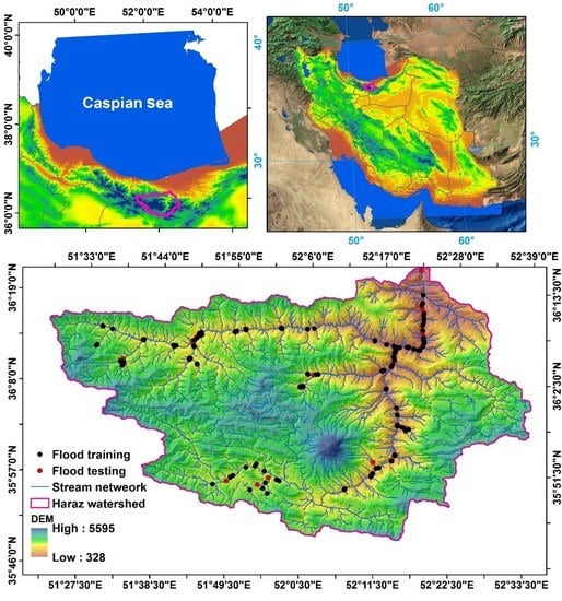
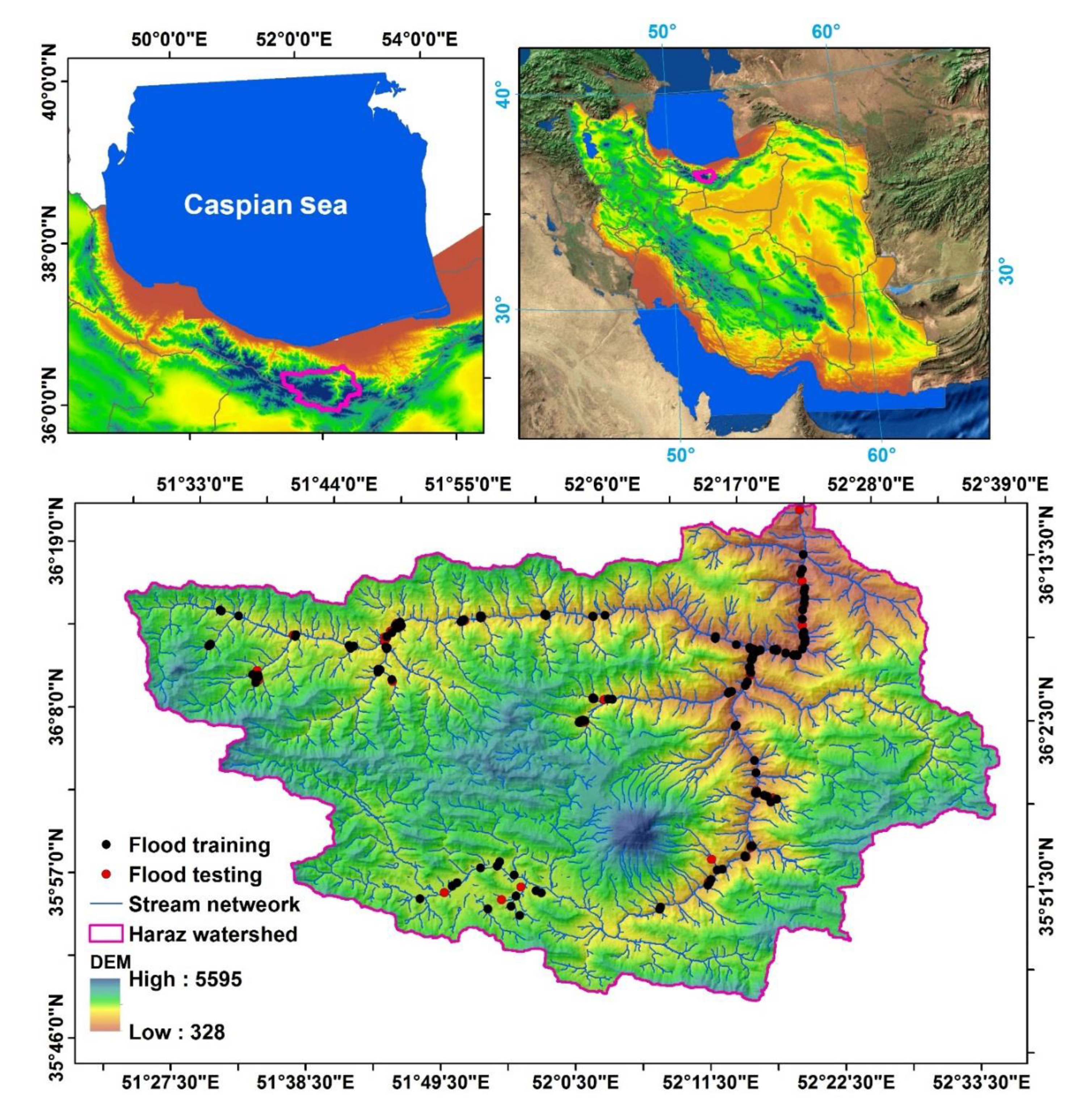
2. Description of Study Area
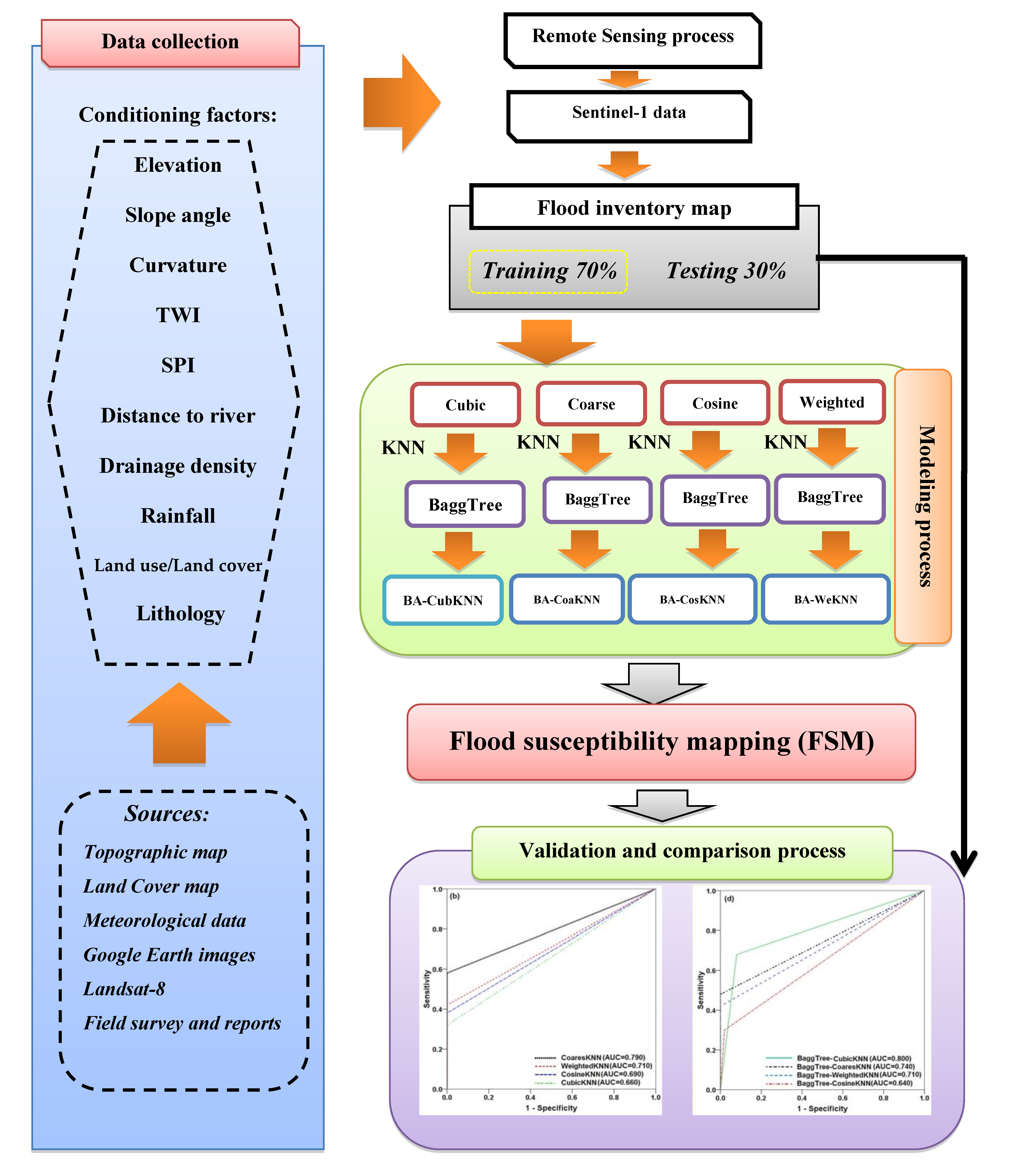
The Haraz watershed is located in Mazandaran Province in northern Iran (Figure 1). The 4015 km2 watershed is mountainous, ranges in elevation from 328 m to 5595 m asl, and has cold winters and mild humid summers with mean annual rainfall of 430 mm [16]. Factors that contribute to flooding here include rainfall, deforestation, land-use changes, and inadequate flood management policies [53]. GIS data show that slopes in the watershed range up to 66°, with 5% flat terrain and 95% hilly and mountainous terrain [8]. Most of study area (92%) is rangeland. The ground is rocky and dominantly developed on Jurassic formation [16]. Haraz has a long history of catastrophic flooding. In April 2019, floods in Mazandaran Province killed six people, damaged more than 200 villages, and caused USD $166.4 million damage to agriculture [16]. Thus, there is a pressing need for more reliable flood hazard maps for this area.

3. Methodology

The flowchart for the methodology used in this study is shown in Figure 2. The workflow includes: (1) data collection and preparation, which involves determining appropriate conditioning factors (factor ranking and selection); (2) preparation of a flood inventory map; (3); modeling flood susceptibility with KKN functions and its ensembles using the Bagging Tree algorithm; (4) preparation of flood susceptibility maps; and (5) validation and comparison of the models and flood susceptibility maps using training (goodness-of-fit) and validation (prediction accuracy) datasets.

3.1. Data Acquisition

3.1.1. Flood Inventory Map

We mapped flooded areas using Sentinel-1 images, remote sensing data and field surveys. In this study, a flood inventory was assembled based on flood events in 2008, 2012, 2016, and 2017. We also used flood event data collected by the Mazandaran Regional Water Authority (MRWA), aerial photographs, Google Earth, and field surveys. To prepare our flood map, we chose 201 flood points and 201 nonflood points, of which we used 70% for training (141 points) and 30% for validation (60 points). Both flood and nonflood points are needed for flood susceptibility modelling [11,79].

3.1.2. Flood Conditioning Factors

A variety of flood conditioning factors should be tested in flood susceptibility modelling [11]. We chose the following 10 conditioning factors (Table 1) for our study [80] and mapped them at 30-m spatial resolution [30]: distance to river, elevation, slope, lithology, curvature, rainfall, topographic wetness index (TWI), stream power index (SPI), land use/land cover, and river density. We quantified topographic and hydrological factors using an Advanced Space-borne Thermal Emission and Reflection Radiometer (ASTER) DEM. Relevant details for the 10 conditioning factors are described below and in Table 1:

Slope

Higher slope angles increase water velocity and surface runoff [81] and reduce infiltration. Lower slope angles are associated with greater flood depths [82]. We classified slope angle based on the manual classification method into five categories: 0°–5°, 5°–10°, 10°–15°, 15°–25°, and > 25°.

Elevation

Lower elevations are receiving areas for runoff and generally have a higher potential for flooding [82] than higher elevation areas [83]. In this study, we classified elevation using the natural breaks classification method and defined the following nine categories: 328–350, 350–400, 400–450, 450–500, 500–1000, 1000–2000, 2000–3000, 3000–4000, and >4000 m.

Curvature

Water flow is affected by slope curvature [84]. A zero curvature value generally has more potential for flooding than positive and negative curvature values. Most flood-prone areas in the Haraz watershed have zero curvature values associated with flat landforms. We classified curvature using the natural breaks classification method and defined three categories: convex (negative values), flat (zero value), and concave (positive values).

Stream Power Index

Stream power index (SPI), which is a measure of the erosive power of water flow, is defined by the followed equation [85]:
S P I = ( A S × tan β )
where AS is the specific area in m2/m and β is the slope angle in degrees. SPI is related to fluvial processes such as sediment transport and river channel erosion [86]. Fuller [87] found that a high SPI value in confined channels can lead to severe channel transformation. It is generally accepted that an increase in SPI corresponds to an increased likelihood of flooding. We classified SPI using the manual classification method with nine categories: 0–80, 80–400, 400–800, 800–2000, 2000–3000, and >3000.

Topographic Wetness Index

The topographic wetness index (TWI) is a measure of the tendency for water to accumulate at any location within a catchment under the influence gravity and is an important attribute in flood susceptibility mapping [87,88,89,90,91]. It generally reflects spatial soil moisture patterns related to floodplains [90]. Moore et al. [87] proposed the following equation to calculate TWI:
T W I = I n ( A S / tan β )
We classified SPI using the natural breaks classification method with six categories: 1.9–3.94, 3.95–4.47, 4.48–5.03, 5.04–5.71, 5.72–6.96, and 6.97–11.53.

Lithology

Lithology can affect flooding through the differences in permeability of rocks and sediments [17]. We obtained a geology layer in GIS shapefile format, which was originally prepared by the Iran Geological Survey Department, from the Mazandaran Regional Water Organization. We created three geologic units: Paleozoic rocks (4.7% of watershed), Mesozoic rocks (56.4%), and Cenozoic rocks and sediments (38.9%).

Rainfall

Rainfall has an obvious and direct effect on flood occurrence [9,16,17,37,92] and, for flood susceptibility mapping, is most commonly expressed as annual rainfall [93]. We quantified the rainfall factor based on 20 years of precipitation data (1991–2011) from 17 stations inside and outside the study area. We selected a simple kriging method to create the rainfall layer because it produced the lowest root mean square error (RMSE) and mean absolute error (MAE) [2]. We divided the rainfall layer into six classes: 183–333, 334–379, 380–409, 410–448, 449–535, and 536–741 mm [86].

Land Use/Land Cover

Land use/land cover has an important role in flooding. For example, runoff increases when vegetated land is converted to bare land [94]. We extracted land use/land cover from the operational land imager (OLI) of Landsat 8 scenes acquired in 2013 using the land-use unit classification method in ArcGIS 10.3 and supervised classification in Environment for Visualizing Images (ENVI 5.1) software. Our seven land use/land cover classes are: water bodies, residential areas, grassland, garden, farm land, forest land, and barren land.

River Density

River density is a measure of the number of streams and rivers in an area. If all other conditioning factors are constant, high river densities have a higher potential for flooding than low river densities [8]. We classified river density using the natural breaks classification method and defined six categories: 0–0.401, 0.401–1.17, 1.92–2.67, 2.67–3.66, and 3.66–7.3 km/km2.

Distance to River

Distance to river (i.e., distance of the measurement points from the river) plays a major role in the distribution and magnitude of floods in the study area [95]. The shorter the distance, the higher the probability of flooding, especially where the river has a low storage capacity [96,97]. To create the distance-to-river layer, we edited the digital watershed map using the multi-ring buffer command in ArcGIS 10.3. Generally, low infiltration rates in the Haraz watershed result in rapid runoff in the vicinity of rivers during high-intensity rainfall events, which in turn causes catastrophic flooding in areas with low topographic gradients [28]. We divided distances to river into eight classes: 0–50, 50–100, 100–150, 150–200, 200–400, 400–700, 700–1000, and >1000 m.

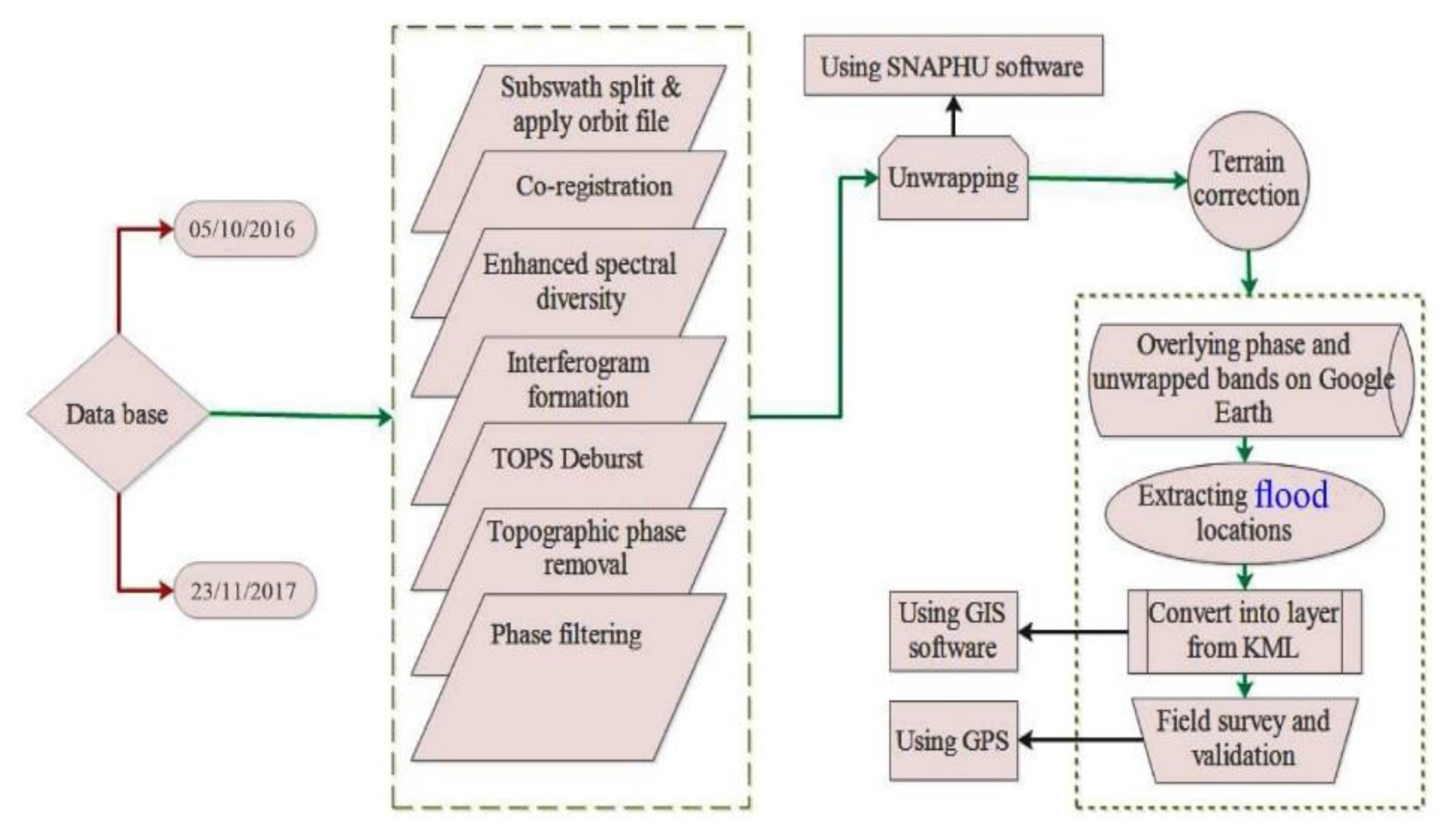
3.2. Detection of Flood-Prone Area by Sentinel-1

Sentinel-1 is the first satellite constellation of the European Space Agency’s Copernicus Programme and comprises two satellites that share the same orbital plane—Sentinel-1A and Sentinel-1B. They carry a C-band (5.7 cm wavelength) synthetic radar instrument, which collects data in all weather, day or night. The radar has four different operational modes: strip map (SM), wave (WV), interferometric wide swath (IW), and extra wide swath (EW). Its main drawback is that radar waves cannot penetrate dense vegetation [98].
The backscatter signal from inundated areas is identifiable in Sentinel-1 SAR data products, which are freely available through the Sentinel Scientific Data Hub (scihub.copernicus.eu). The specular reflection of C-band signals over flooded areas is significantly lower than over bare ground in the present study, Sentinel-1 Level-1 Ground Range Detected (GRD) data were projected onto the ground using an Earth ellipsoid model (WGS84). Finally, we used Sentinel-1 SAR data to identify and map flooded areas using the InSAR method [99,100,101].

Data Preprocessing and Processing

The process of flood detection using Sentinel-1 data includes the following steps:
Step 1:Radar data acquisition. We used Sentinel’s Application Platform (SNAP) to manipulate radar data, as well as threshold data acquired during the flood (Table 2).
Step 2: Radar data preprocessing: We coregistered radar images using the coherence between master and slave images [102]. We selected two images from 05/10/2016 and 23/11/2017 as the master images. We combined a split su-swath and applied the orbit file technique to extract the boundary of the study area. We then overlaid the coregistered radar data. Next, we enhanced the spectral resolution of the radar images using a spectral diversity technique.
We produced an interferogram by multiplying the values of pixels in the master image and the conjugate complex number of related pixels in the slave image [102,103]. To detect flood-prone areas, we applied pre- and post-flood data by the interferogram formation technique.
We identified zones of terrain observation progressive scan (TOPS) data [104]. Data within these zones were considered to be invalid and thus were removed. Removal of the topographic phase provided an interferogram [102,104,105] that allowed us to specify nonflood-prone areas. Finally, we used phase filtering to detect flood-prone.
Step 3: Radar data processing. We used the output from step 2 as input for processing the digital images with SNAPHU and ENVI 5.1 software. We used ArcGIS 10.3 to analyze spatial data (Figure 2). We viewed the phase and the unwrapped and the coherence bands in Google Earth to identify and record historical flood locations. We used a handheld GPS in the field to validate the extracted flood-prone locations, 40% of which were near the main rivers. Finally, we verified the accuracy of Google Earth images and the radar data, and vectorized points using ArcGIS 10.3 software. For georeferencing, we employed ground control points (GCPs), nearest neighbor resampling, and a first-order transformation (Figure 3).

3.3. Background of Flood Susceptibility Models

3.3.1. K-Nearest Neighbor Classifier

K-Nearest Neighbor (KNN) is a common classification tool used in data mining applications [106]. It is a nonparametric, lazy learning algorithm that makes no assumptions about the primary dataset. This is important when modeling hydrological processes, such as floods and stream flow, for which there is little or no prior knowledge of the data distribution [107]. In addition, these processes are nonlinear and heterogeneous with noisy data that challenge common statistical assumptions such as those underpinning linear regression models [108]. In this context, KNN is a useful tool as it uses all contributing cases in the dataset and classifies new cases based on their similarity indices (also called ‘distance functions’). Cases are classified by voting for neighbor classes. The optimal case is the one with the highest similarity indices [109].
In KNN, the optimal choice of the chosen number of neighbors (K) depends on the metrics used for classification and regression purposes. In the case of continuous variables, the most common distance metric is Euclidean distance, also known as the straight-line distance. Conversely, for discrete variables, the overlap metric (or Hamming distance) is frequently used. Other metrics that have been used are correlation coefficients, such as the Pearson and Spearman correlation coefficients. The K value is sensitive to the chosen dataset and differs between datasets. Based on an empirical rule-of-thumb introduced by Dude [110,111], K is equal to the square root of the number of samples; this makes parameter tuning difficult for diverse applications.
There are other popular methods, such as K-fold Cross-Validation (CV), Leave-one-Out Cross-Validation (LOOCV), and bootstrapping. K-Fold Cross-Validation can be used to evaluate the test error with a statistical learning method. This approach places randomly chosen sets of observations into K folds of equal size. In contrast, LOOCV does not use two sets of equal size; rather, it employs a single observation for the validation set and the remaining observations for the training set. We use these two methods as well as bootstrapping to measure the accuracy of our statistical learning approach. However the K-fold Cross-Validation method is preferred for the following reasons [112]:
  • There are typically only a few probable choices of K (e.g., from 3–10 or 50–100).
  • The K-fold CV offers a greater computational advantage than other methods.
  • The K-fold CV yields more accurate estimates of the test error than bootstrapping and LOOCV.
With K-fold CV, the training phase is short and fast. All training datasets are required during the testing phase to decide on the best subset of the entire training dataset. This method has been used in diverse applications such as big data classification, pattern recognition, ranking models, and computational geometry [106].
The K-fold CV algorithm applies a vector as an input to the K training dataset. It then uses the most common class to classify the K nearest neighbors. During the training phase, neighbors are defined based on their distances from the test dataset; the classes of the test dataset are determined in the testing phase [4]. The number of neighbors can be changed to determine the best performance of the KNN algorithm. There are four KNN classifiers introduced by MATLAB [113]:
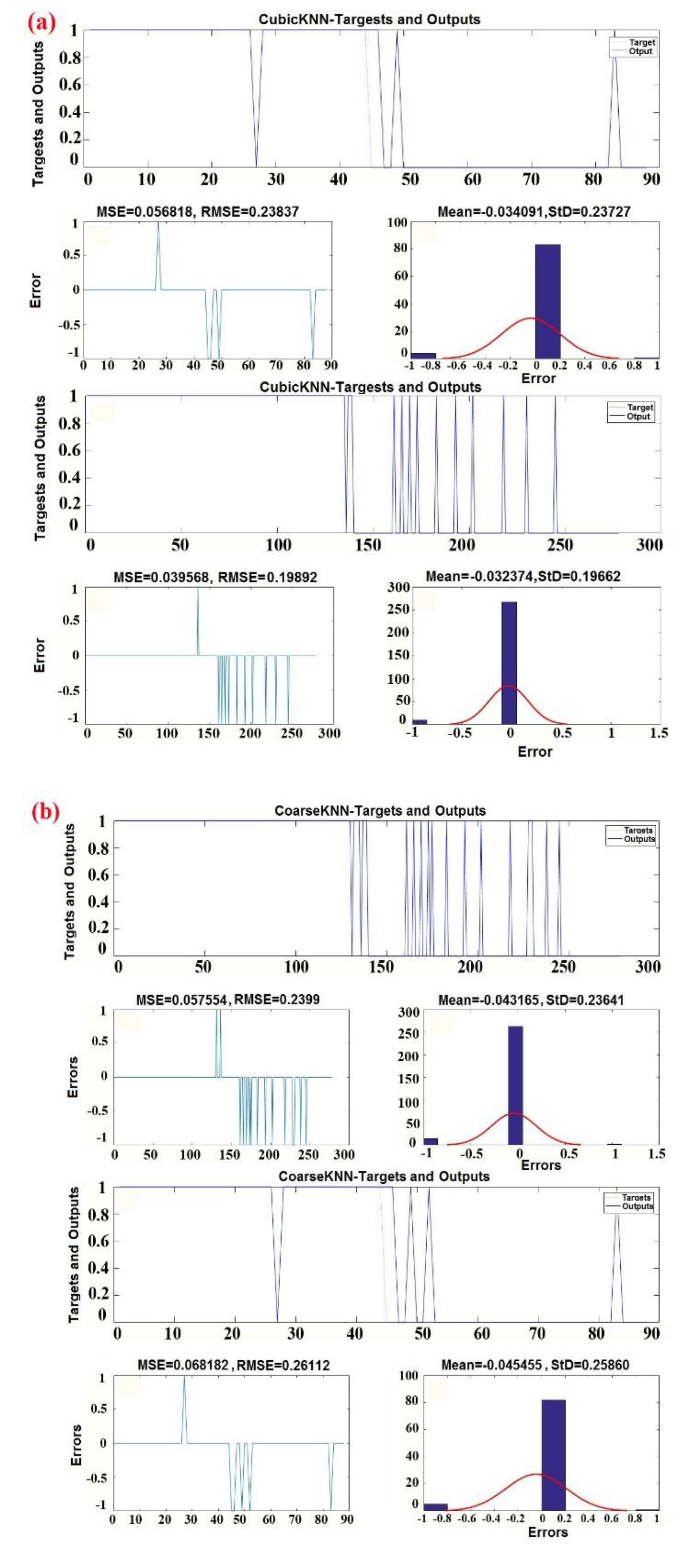
  • Coarse KNN: The number of neighbors is 100. The classifier is defined as the nearest neighbor among all classes.
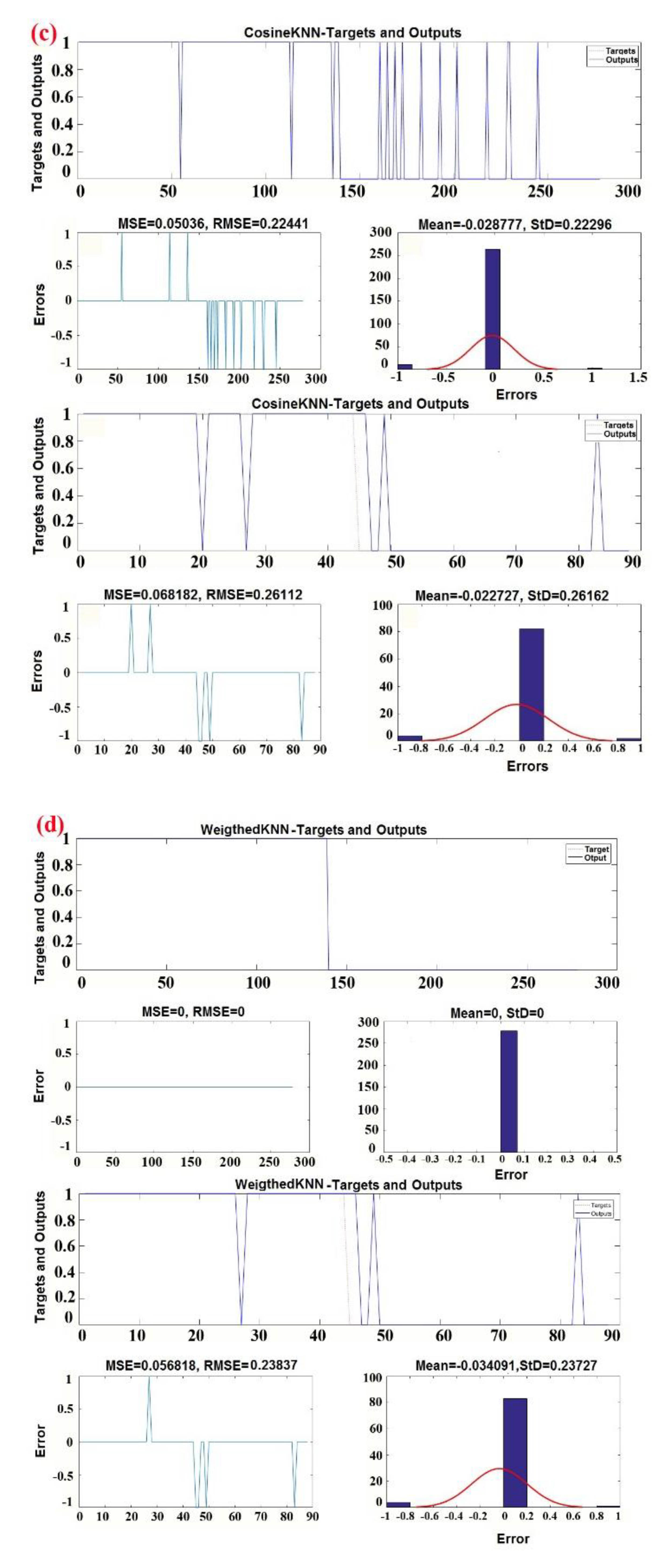
  • Cosine KNN: The cosine distance metric is the nearest neighbor classifier. It is generally used as a metric for distances when vector magnitudes are irrelevant. The following equation is used to measure the distance between two vectors, u and v [113]:
    1   u . v | u | . | v |
  • Cubic KNN: The number of neighbors is 10, and the cubic distance metric is the nearest neighbor classifier [109]. The following equation is used to measure the distance between two n-dimensional vectors, u and v:
    i = 1 n | u i v i | 3
  • Weighted KNN: The number of neighbors is 10, and the weighted Euclidean distance is used as the nearest neighbor classifier. The following equation is used to measure the weighted Euclidean distance between two n-dimensional vectors, u and v:
    i = 1 n w i ( x i y i ) 2
    where 0 < w i < 1 and i = 1 n w i = 1 .

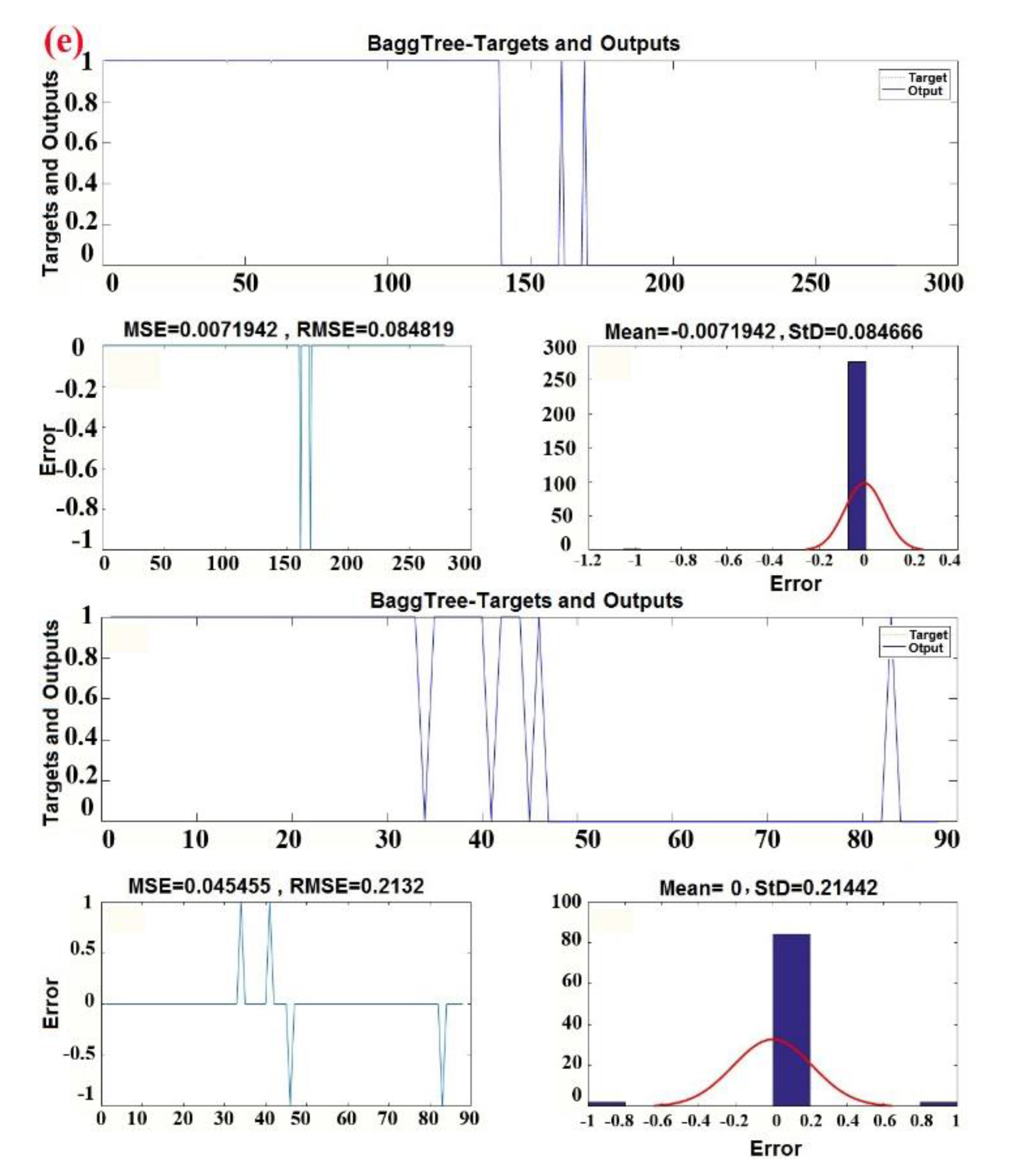
3.3.2. Bagged Tree Ensemble Algorithm

Ensemble methods apply a variety of decision trees, instead of only one, to improve predictive performance. The two most common techniques used with ensemble models are [114] bagging and boosting.
Bagging (Bootstrap Aggregation) improves the precision and consistency of machine learning algorithms used for regression and statistical classification. The purpose of bagging is to decrease variance while retaining the bias of a decision tree and preventing overfitting. The Bagging Tree randomly generates multiple sets of input data from training samples by replacement [115]. The chosen subset data are used to train the assigned trees and generate models. Subsequently, the average of all predictions from these trees is used to make the final decision with a higher degree of robustness. The accuracy of a single tree is increased by using multiple copies of the trained subset of data.
Boosting is a useful ensemble method in high bias situations. Predictors are trained sequentially with simple training models, and the data are then analyzed for errors. At every step, the net error is calculated from the prior decision tree [115]. In a high bias dataset for which an input is not well classified by an hypothesis, its weight is amplified so that next hypothesis will classify it properly.
For the present study, we used the Bagging Tree ensemble method on a well classified set of inputs with low bias. The method yields results with a lower variance than its components, which in turn makes the learning procedure more efficient. The best classifier type depends on the training dataset. In the current study, we employed a classifier that provides the optimum tradeoff in memory, speed, interpretability, and flexibility.
We subdivided the dataset into two probable classes and generated an algorithm of continuous classifiers ( H m , = 1     M ) H m :   D m     R on a training set (flood collection) D. We then grouped the generated classifiers into a composite classifier with a resulting prediction weight as follows:
H ( d i ) = s i g n ( m = 1 M α m H m ( d i ) )   , where   sign   is : s i g n   ( x ) = { 1   ,   x > 0 0   , x = 0 1   ,   x < 0
Equation (6) describes a voting procedure known as majority (plurality) voting for each classifier. Plurality voting efficiently attains the optimum tradeoff in error and rejection rate. An example d i is classified based on the majority of classifier votes [116,117,118]. a m ,   m = 1 , , M are parameters that indicate the impact of more accurate classifiers on the final result. H m are termed ‘weak classifiers’ because their accuracy is higher than the accuracy of other random classifiers [119].
We used the following bagging algorithm in our study [120]:
  • Training set D initialization.
  • Range selection for m = 1, …, M.
    2.1.
    Random selection of the set D to create a new set D m   .
    2.2.
    Machine-learning application on the base of D m   to train a classifier H m :   D m     R .
  • Creation of a composite classifier H from H m ,   m = 1 , , M .
    3.1.
    d i classification based on c i   classes, depending on the number of votes gained from
    H m   H ( d i ,   c i ) = s i g n ( m = 1 M α m H m ( d i ,   c i ) )   ,   where   sign   is   : s i g n   ( x ) = { 1   ,   x > 0 0   , x = 0 1   ,   x < 0
We note that to achieve a better performance and decrease the classification error, the H m values can be reformed, while α m values remain constant.

3.3.3. Proposed New Ensemble Machine Learning Models of Bagging with KNNs Functions

We used the Classification Learner application in MATLAB R2018a to automatically train a selection of different KNN classification models on a training dataset. Then we used the Bagging Tree ensemble together with the coarse, cosine, cubic, and weighted KNN base classifiers to spatially predict floods. For a given training set, we produced multiple different training sets (‘bootstrap samples’) from replacement samples from the original dataset. Then, we built KNN models for each bootstrap sample. The result is an ensemble of models, where each model votes with equal weight. The goal of this procedure is to reduce the variance of the model of interest.

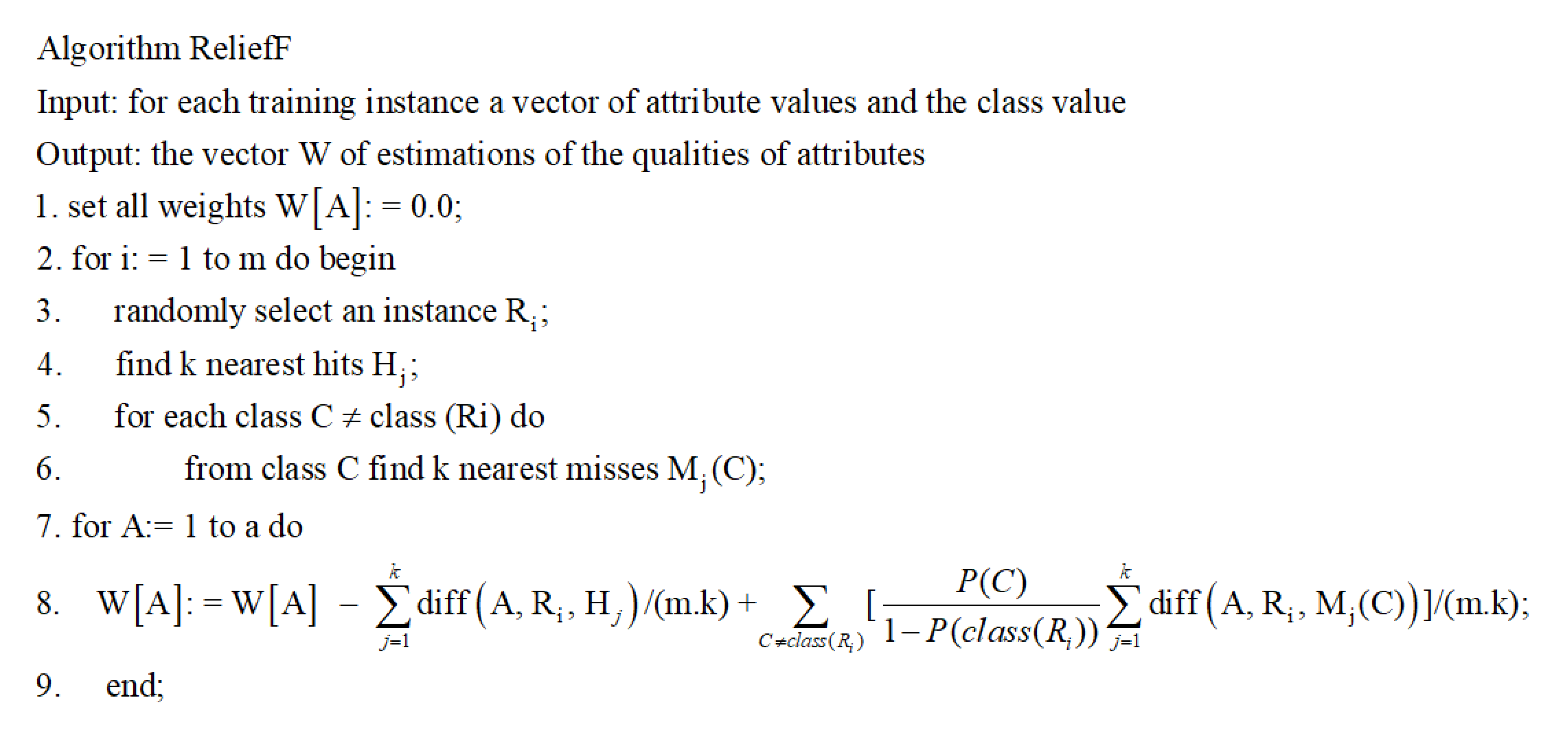
3.3.4. Flood Factor Selection Using the Relief Attribute Evaluation (RFAE) Technique

Supervised machine learning algorithms rely on the selection of the best factors or features to accurately classify sample data and enhance the efficiency of training [121]. The main aims of factor and feature selection are to enhance the learning efficiency of the modelling process and the robustness of predictive accuracy, and to reduce complexity, noise, and overfitting by eliminating irrelevant or low-performing factors [122]. Conditioning factors can be evaluated and categorized based on a variety of metrics, including distance, information, dependency, consistency, and classifier error rate [123]. In this study, we selected the Relief Attribute Evaluation (RAE) technique to check the importance of conditioning factors on flood classification performance (Figure 3). RAE is a distance-based attribute/factor ranking approach proposed by Kira and Rendell [124], and later improved by Kononenko [125] and Hall and Holmes [126]. It calculates the class of each attribute based on the distance between the data point and its nearest neighbors (Figure 4). First, it randomly selects instances in the training dataset (Ri in line 3 of Figure 4). Then, it searches for K of its nearest neighbors from the same class, as well as from each of the different classes, called nearest hit Hj and nearest miss (Mj(C) (lines 4 and 6, respectively). Depending on the average values of Ri, Hj, and Mj (C) (lines 7, 8, and 9), RAE updates the quality estimation W[A] for all attributes. W[A] is reduced when instances Ri, and Hj have different values of attribute A. To obtain a desired value, attribute A is separated into two instances with the same class values. If Ri and Mj (C) have different values of attribute A, attribute A is divided into two instances with different class values. The prior probability for each class of misses, P(C), is calculated based on the training dataset. P(C) is symmetric and ranges from 0 and 1 for hits and misses. If the sum of the class is missing, its probability weight is divided by factor 1-P (class (Ri)) to represent its probability sum. This process is repeated m times. The quality of a flood attribute is evaluated based on how well it distinguishes nearby instances. Weights for all attributes are assigned by the ReliefF algorithm through iterative estimation using the nearest hit-and-miss neighbors. Accordingly, an attribute is ranked highest if the same value is obtained for instances of the same class and distinguished for instances of different classes [127,128].

3.4. Evaluation and Comparison

New models should be tested to verify their performance and evaluate their potential applicability in other regions. For the purpose of validation, an objective function (‘forecasting error’), such as mean square error (MSE) and root mean square error (RMSE), can be used to find the difference between observed and predicted values. Although there are a variety of error indices that can be used to assess the predictive capability of the models, many studies advocate the use of RMSE as a standard metric for model errors in geosciences [129]. MSE and RMSE can be formulated as follows:
M S E = 1 n i = 1 n ( F e s t . F o b s . ) 2
R M S E = 1 N i = 1 N ( F e s t . F o b s . ) 2
where F e s t . , F o b s . and n are respectively, estimated floods, observed (actual) floods, and the number of floods for the modelling process.
In addition to MSE and RMSE, we used accuracy, the receiver operatic characteristic curve (ROC), and the area under the ROC curve (AUC) to further evaluate the predictive capability of the models. The accuracy metrics are formulated based on true positive (TP), true negative (TN), false positive (FP), and false negative (FN) values. TP and TN are the number of flood pixels that are correctly classified as flood and nonflood pixels, respectively [37,52]. FP and FN are the number of nonflood pixels that correctly classified as nonflood and flood pixels, respectively [16,17]. Accuracy can be formulated as follows:
A c c u r a c y = T P + T N T P + T N + F P + F N
The ROC curve has been used in some flood modeling studies to check the overall performance of models [8,39,40,130]. It is plotted using two statistical metrics—specificity on the x axis and sensitivity on the y axis [63]. Specificity and sensitivity are defined, respectively, as the number of incorrectly and correctly classified floods [92]. An AUC equal to 1 indicates that the model is perfect or ideal, whereas a value of 0 indicates an inaccurate model [3].
A U C = T P + T N M + N
where M and N are the number of total flood and nonflood pixels [131].

4. Result and Analysis

4.1. Flood Detection Using AIRSAR and Optical Satellite Images

Using the InSAR technique and SNAP software, we generated coherence, unwrapped, and phase bands from Sentinel-1 satellite imagery dating to between 05/10/2016 and 23/11/2017. The highest and lowest values in the phase and unwrapped bands were mapped and depicted on maps in red and green colors. The coherence band provided the best results because white areas (high values) can be clearly distinguished from stable areas (low values). The InSAR-generated coherence, phase, and unwrapped bands were then transformed into KML format and draped on Google Earth (GE) images to digitize flood locations. Our Sentinel-1-derived flood polygons are in good agreement with our field survey observations (Figure 5).

4.2. The Most Important Factors for Flood Modelling

The results of factor selection by the RFAE technique are shown in Figure 6. The average merit (AM) values range from 0.002 to 0.198, indicating different strengths of individual conditioning factors for flood susceptibility modelling. Intuitively, distance to river has the highest average merit (AM = 0.198) because most flood points are near rivers and streams. The other factors, in order of decreasing importance are slope (AM = 0.186), curvature (AM = 0.160), drainage density (AM = 0.150), elevation (AM = 0.135), TWI (AM = 0.124), lithology (AM = 0.059), rainfall (AM = 0.053), SPI (AM = 0.043), and land use/land cover (AM = 0.002).

4.3. Flood Modelling Process

The Bagging Tree and Modified K-Nearest Neighbor classifiers (Cubic–KNN, Coarse–KNN, Cosine–KNN, and Weighted–KNN) were used in this study for flood modelling. We trained and tested the models with, 70% and 30% of our dataset, respectively. We calculated the accuracy criteria of the models by comparing the training/test dataset with predicted flood pixels as output (Figure 7). In the training step, the MSEs of the Cubic–KNN, Coarse–KNN, Cosine–KNN, Weighted–KNN, and Bagging Tree models are 0.0568, 0.0575, 0.0504, 0.000, and 0.0072, respectively; the corresponding RMSEs are 0.2383, 0.2399, 0.2244, 0.0000, and 0.0848. These results show that the Weighted–KNN model had the best performance in the training step (mean = −0 and standard deviation = 0). In the test step, the MSEs and RMSEs of the Cubic–KNN, Coarse–KNN, Cosine–KNN, Weighted–KNN, and Bagging-Tree models are, respectively, 0.0396 and 0.1989, 0.0682 and 0.2611, 0.0682 and 0.2611, 0.0568 and 0.2384, and 0.0454 and 0.2132. These results suggest that the Cubic–KNN model performed best in the test step (mean = −0.0324 and standard deviation = 0.1966).
We also evaluated the accuracy of the KNN classifier functions in the modelling process. Table 3 shows the optimum parameters for achieving the highest model accuracy. The Cubic–KNN model has the highest accuracy value (96.4%), followed by the Cosine–KNN (92.8%), Weighted–KNN (92.14%), and Coarse–KNN (92.1%) models. We also built hybrid models of Bagging Tree based on KNN classifiers and derived their optimum parameters based on the highest accuracy. Table 4 shows the optimum parameter values of the hybrid models. We obtained the highest accuracy for the hybrid model of Bagging Tree–Coarse KNN (98.6%), followed by Bagging Tree–Weighted KNN (97.1%), Bagging Tree–Cosine KNN (96.6%), and Bagging Tree–Cubic KNN (94.3%).

4.4. Development of Flood Susceptibility Maps

We used the hybrid methods to evaluate the flood susceptibility index (FSI) in all pixels in our study area. Each pixel was given a unique FSI, and the results then were exported into a readable ArcGIS 10.3 format for the task of flood mapping. We classified the calculated FSIs into flood and nonflood classes. Figure 8 shows flood susceptibility maps produced by the Bagging Tree ensemble and based on Modified K-Nearest Neighbor classifiers. The maps show that flood-prone areas in the watershed are located near rivers at lower elevations and on low-gradient slopes. Figure 8b,d; Figure 8b; Figure 8d,f,h show that the Bagging Tree ensemble model can enhance and extend flood-prone areas adjacent to rivers such that most known flood locations are located in high and very high susceptibility classes. In addition, Figure 8 shows that areas near the outlet of the Haraz watershed, as well as areas in the northwest part of the catchment, are more prone to flooding than other parts of the study area. In comparison to the nearest neighbor models, the hybrid models predict that higher proportions of the study area are flood susceptible (Figure 8). Of the hybrid models, the Bagged Tree–Cubic KNN model (Figure 8b) has the largest flood-prone area.

4.5. Evaluation and Comparison

We next compared the flood susceptibility performance of the new hybrid Bagging Tree–KNN models with that of the KNN models using the area under receiver operating characteristic (AUC) curve. Figure 9 shows the AUC of ROC curves that we produced for the training and testing steps of our flood susceptibility map datasets. The AUC curves show that the Coarse–KNN model performed best in the training and testing steps, with AUC values of 0.795 and 0.790, respectively. It is followed by the Weighted–KNN model (AUC = 0.719 and 0.710), Cosine–KNN model (AUC = 0.692 and 0.690), and the Cubic–KNN model (AUC = 0.662 and 0.660) (Figure 9a,b). Among the hybrid models, the Bagging Tree–Cubic KNN model had the highest performance in both the training and testing steps, with AUC values of 0.811 and 0.800, respectively. It is followed by the Bagging Tree–Coarse KNN model (AUC = 0.762 and 0.740), the Bagging Tree–Weighted KNN model (AUC = 0.722 and 0.710), and the Bagging Tree–Cosine KNN model (AUC = 0.659 and 0.640) (Figure 9c,d). The hybrid models outperformed the KNN classifier models. This result accords with the conclusion of Kantardzic [132] that the Bagging Tree–Cubic KNN model performs better than rival models (Figure 9). We therefore recommend that our highest performing model, the Bagging Tree–Cubic KNN model, be tested for flood susceptibility modelling in other areas.

5. Discussion

Flood susceptibility maps can be used by a variety of decision-makers and hazard managers to reduce injury and damage to built infrastructure from floods. We found that Sentinel-1 radar data are useful for mapping flood extent. In terms of flood susceptibility modelling, the task of choosing the best-performing machine learning algorithm can be difficult due to data complexity [102]; it commonly requires a trial-and-error approach. In our study area, the best performing model is a new intelligent hybrid model (Bagging Tree–Cubic KNN), which is a combination of a bagging ensemble technique and the four functions of the KNN classifier. We used the information gain ratio (IGR) on our ten flood conditioning factors and showed that, although all factors are significant in the model training, distance to a river stands out as the most important factor, followed by slope gradient and curvature. Our results are in agreement with those of Ahmadlou et al. [130], Bui et al. [39], Khosravi et al. [3], and Shafizadeh-Moghadam et al. [40]. As most floods in the Haraz watershed result from brief heavy rainfall and overbank river flow, it follows that areas adjacent to rivers and floodplains have the greatest flood susceptibility.
The KNN model is one of the most popular neighborhood classifiers; it is very simple to use and highly efficient in some fields of studies [133]. Computer memory requirements and operation time are the main limitations of KNN classifier performance, because this classifier depends on every example in the entire training set [134]. To solve these limitations and increase the performance of KNN, we used a bagging meta classifier. The combination of the Bagging Tree ensemble method and the KNN classifier allowed us to overcome the above-mentioned limitations and develop a reliable flood model. The AUC value (0.800) of the proposed Bagging Tree–Cubic KNN model indicates that its performance is best. This hybrid model may significantly improve the prediction accuracy of Cubic KNN as a base classifier.
Chapi et al. [8] tested and evaluated the bagging ensemble method to improve the power prediction of the logistic model tree (LMT) classifier in a new model (Bagging–LMT) for flood mapping in the Haraz watershed. They concluded that bagging increases the power prediction of the LMT base classifier in flood modelling. The ensemble model outperforms the basic classifier due to the synergy provided by the two classifiers when used together. We therefore recommend the proposed new model as an appropriate method for flood hazard management.
Flood modelling is a complex procedure with numerous uncertainties. Machine learning approaches efficiently handle these uncertainties as long as reliable historical flood inventory maps are available. The proposed machine learning model provides decision makers with a less expensive and less time-consuming way of evaluating flood hazards and risk than field surveys. It also provides authorities guidance as to what additional data (e.g., rainfall and river discharge data) might be required to produce more accurate flood maps for mitigating further damage. The flood susceptibility maps are thus fundamental products for further analyses and for hazard and risk disaster management and mapping. Our model may be used in other areas aside from the Haraz watershed.

6. Conclusions

The best way to mitigate and control floods is to identify all factors that have a relationship to flooding; in this study, we refer to these as conditioning factors. We used Sentinel-1 remote sensing radar data to identify and map flood locations in the Haraz watershed in northern Iran. We used 10 flood conditioning factors and 201 flood locations as our model inputs. Eight new hybrid models (Cubic–KNN, Bagging Tree–Cubic KNN, Coarse–KNN, Bagging Tree–Coarse–KNN, Cosine–KNN, Bagging Tree–Cosine–KNN, Weighted KNN, and Bagging Tree–Weighted KNN) were created to analyze and map flood susceptibility. Results based on the relief attribute evaluation metric indicate that distance from the river and slope gradients are the two most important factors for flood occurrence in the Haraz watershed. Among the eight models, we found that Bagging Tree–Cubic KNN model has the highest predictive power.
Flood modeling is a complicated task with many uncertainties, but we have shown that machine learning algorithms can improve flood susceptibility mapping. Our proposed flood model is effective, simple and intuitive. It reduces the variance and the noise of the training dataset, resulting in enhanced prediction accuracy. Our method of combining satellite radar data with the Bagging Tree–Cubic KNN model should be evaluated in other flood-prone regions, especially in large catchments where collecting data in the field is difficult and commonly expensive. This machine learning model can be used to improve the efficiency and accuracy of flood hazard mapping and thus assists in disaster management and land-use planning.

Author Contributions

H.S., A.S., K.G., E.O., N.A.-A., J.J.C., M.G., K.K., A.A., S.B., K.H., H.N., O.R., K.H., A.M., H.N., A.M.M., B.B.A., and A.A. contributed equally to the work. H.S., A.S., and K.K. collected field data and performed the flood susceptibility mapping and analysis. H.S., A.S., N.A.-A., K.G., E.O., K.K., S.B., K.H., and O.R. wrote the manuscript. N.A.-A. contributed, analyzed and interpreted data. M.A., J.J.C., M.G., H.N., K.H., A.M., A.A., H.N., A.M.M., N.A.-A., B.B.A., and A.A. helped plan and edit the manuscript. All authors have read and agreed to the published version of the manuscript.

Funding

Our research was supported by the Iran National Science Foundation (INSF) through research project no. 96004000.

Conflicts of Interest

The authors declare no conflict of interest.

References

  1. Hirabayashi, Y.; Mahendran, R.; Koirala, S.; Konoshima, L.; Yamazaki, D.; Watanabe, S.; Kim, H.; Kanae, S. Global flood risk under climate change. Nat. Clim. Chang. 2013, 3, 816. [Google Scholar] [CrossRef]
  2. Khosravi, K.; Nohani, E.; Maroufinia, E.; Pourghasemi, H.R. A gis-based flood susceptibility assessment and its mapping in iran: A comparison between frequency ratio and weights-of-evidence bivariate statistical models with multi-criteria decision-making technique. Nat. Hazards 2016, 83, 947–987. [Google Scholar] [CrossRef]
  3. Khosravi, K.; Pham, B.T.; Chapi, K.; Shirzadi, A.; Shahabi, H.; Revhaug, I.; Prakash, I.; Bui, D.T. A comparative assessment of decision trees algorithms for flash flood susceptibility modeling at haraz watershed, northern iran. Sci. Total Environ. 2018, 627, 744–755. [Google Scholar] [CrossRef]
  4. Kron, W. Keynote lecture: Flood risk = hazard × exposure × vulnerability. Flood Def. 2002, 30, 82–97. [Google Scholar]
  5. Messner, F.; Meyer, V. Flood damage, vulnerability and risk perception–challenges for flood damage research. In Flood Risk Management: Hazards, Vulnerability and Mitigation Measures; Springer: Berlin/Heidelberg, Germany, 2006; pp. 149–167. [Google Scholar]
  6. Yu, J.; Qin, X.; Larsen, O. Joint monte carlo and possibilistic simulation for flood damage assessment. Stoch. Environ. Res. Risk Assess. 2013, 27, 725–735. [Google Scholar] [CrossRef]
  7. Sarhadi, A.; Soltani, S.; Modarres, R. Probabilistic flood inundation mapping of ungauged rivers: Linking gis techniques and frequency analysis. J. Hydrol. 2012, 458, 68–86. [Google Scholar] [CrossRef]
  8. Chapi, K.; Singh, V.P.; Shirzadi, A.; Shahabi, H.; Bui, D.T.; Pham, B.T.; Khosravi, K. A novel hybrid artificial intelligence approach for flood susceptibility assessment. Environ. Model. Softw. 2017, 95, 229–245. [Google Scholar] [CrossRef]
  9. Tien Bui, D.; Khosravi, K.; Li, S.; Shahabi, H.; Panahi, M.; Singh, V.; Chapi, K.; Shirzadi, A.; Panahi, S.; Chen, W. New hybrids of anfis with several optimization algorithms for flood susceptibility modeling. Water 2018, 10, 1210. [Google Scholar] [CrossRef] [Green Version]
  10. Alfieri, L.; Bisselink, B.; Dottori, F.; Naumann, G.; de Roo, A.; Salamon, P.; Wyser, K.; Feyen, L. Global projections of river flood risk in a warmer world. Earth’s Future 2017, 5, 171–182. [Google Scholar] [CrossRef]
  11. Tehrany, M.S.; Pradhan, B.; Jebur, M.N. Flood susceptibility mapping using a novel ensemble weights-of-evidence and support vector machine models in gis. J. Hydrol. 2014, 512, 332–343. [Google Scholar] [CrossRef]
  12. Ouchi, K. Recent trend and advance of synthetic aperture radar with selected topics. Remote Sens. 2013, 5, 716–807. [Google Scholar] [CrossRef] [Green Version]
  13. Teshebaeva, K.; Roessner, S.; Echtler, H.; Motagh, M.; Wetzel, H.-U.; Molodbekov, B. Alos/palsar insar time-series analysis for detecting very slow-moving landslides in southern kyrgyzstan. Remote Sens. 2015, 7, 8973–8994. [Google Scholar] [CrossRef] [Green Version]
  14. Joyce, K.E.; Belliss, S.E.; Samsonov, S.V.; McNeill, S.J.; Glassey, P.J. A review of the status of satellite remote sensing and image processing techniques for mapping natural hazards and disasters. Prog. Phys. Geogr. 2009, 33, 183–207. [Google Scholar] [CrossRef] [Green Version]
  15. Tien Bui, D.; Shahabi, H.; Shirzadi, A.; Chapi, K.; Alizadeh, M.; Chen, W.; Mohammadi, A.; Ahmad, B.; Panahi, M.; Hong, H. Landslide detection and susceptibility mapping by airsar data using support vector machine and index of entropy models in cameron highlands, malaysia. Remote Sens. 2018, 10, 1527. [Google Scholar] [CrossRef] [Green Version]
  16. Tien Bui, D.; Khosravi, K.; Shahabi, H.; Daggupati, P.; Adamowski, J.F.; Melesse, A.M.; Thai Pham, B.; Pourghasemi, H.R.; Mahmoudi, M.; Bahrami, S. Flood spatial modeling in northern iran using remote sensing and gis: A comparison between evidential belief functions and its ensemble with a multivariate logistic regression model. Remote Sens. 2019, 11, 1589. [Google Scholar] [CrossRef] [Green Version]
  17. Khosravi, K.; Melesse, A.M.; Shahabi, H.; Shirzadi, A.; Chapi, K.; Hong, H. Flood susceptibility mapping at ningdu catchment, china using bivariate and data mining techniques. In Extreme Hydrology and Climate Variability; Elsevier: Amsterdam, The Netherlands, 2019; pp. 419–434. [Google Scholar]
  18. Khosravi, K.; Pourghasemi, H.R.; Chapi, K.; Bahri, M. Flash flood susceptibility analysis and its mapping using different bivariate models in iran: A comparison between shannon’s entropy, statistical index, and weighting factor models. Environ. Monit. Assess. 2016, 188, 656. [Google Scholar] [CrossRef]
  19. Pradhan, B. Flood susceptible mapping and risk area delineation using logistic regression, gis and remote sensing. J. Spat. Hydrol. 2010, 9, 1–18. [Google Scholar]
  20. Al-Juaidi, A.E.; Nassar, A.M.; Al-Juaidi, O.E. Evaluation of flood susceptibility mapping using logistic regression and gis conditioning factors. Arab. J. Geosci. 2018, 11, 765. [Google Scholar] [CrossRef]
  21. Kazakis, N.; Kougias, I.; Patsialis, T. Assessment of flood hazard areas at a regional scale using an index-based approach and analytical hierarchy process: Application in rhodope–evros region, greece. Sci. Total Environ. 2015, 538, 555–563. [Google Scholar] [CrossRef]
  22. Rahmati, O.; Zeinivand, H.; Besharat, M. Flood hazard zoning in yasooj region, iran, using gis and multi-criteria decision analysis. Geomat. Nat. Hazards Risk 2016, 7, 1000–1017. [Google Scholar] [CrossRef] [Green Version]
  23. De Brito, M.; Evers, M. Multi-criteria decision making for flood risk management: A survey of the current state-of-the-art. Nat. Hazards Earth Syst. Sci. Discuss. 2015, 3, 6689–6726. [Google Scholar] [CrossRef]
  24. de Brito, M.M.; Evers, M.; Almoradie, A.D.S. Participatory flood vulnerability assessment: A multi-criteria approach. Hydrol. Earth Syst. Sci. 2018, 22, 373–390. [Google Scholar] [CrossRef] [Green Version]
  25. Khosravi, K.; Shahabi, H.; Pham, B.T.; Adamawoski, J.; Shirzadi, A.; Pradhan, B.; Dou, J.; Ly, H.-B.; Gróf, G.; Ho, H.L. A comparative assessment of flood susceptibility modeling using multi-criteria decision-making analysis and machine learning methods. J. Hydrol. 2019, 573, 311–323. [Google Scholar] [CrossRef]
  26. Leon, A.S.; Kanashiro, E.A.; Valverde, R.; Sridhar, V. Dynamic framework for intelligent control of river flooding: Case study. J. Water Resour. Plan. Manag. 2014, 140, 258–268. [Google Scholar] [CrossRef] [Green Version]
  27. Khosravi, K.; Sartaj, M.; Tsai, F.T.-C.; Singh, V.P.; Kazakis, N.; Melesse, A.M.; Prakash, I.; Bui, D.T.; Pham, B.T. A comparison study of drastic methods with various objective methods for groundwater vulnerability assessment. Sci. Total Environ. 2018, 642, 1032–1049. [Google Scholar] [CrossRef] [PubMed]
  28. Kia, M.B.; Pirasteh, S.; Pradhan, B.; Mahmud, A.R.; Sulaiman, W.N.A.; Moradi, A. An artificial neural network model for flood simulation using gis: Johor river basin, malaysia. Environ. Earth Sci. 2012, 67, 251–264. [Google Scholar] [CrossRef]
  29. Melesse, A.; Ahmad, S.; McClain, M.; Wang, X.; Lim, Y. Suspended sediment load prediction of river systems: An artificial neural network approach. Agric. Water Manag. 2011, 98, 855–866. [Google Scholar] [CrossRef]
  30. Khosravi, K.; Mao, L.; Kisi, O.; Yaseen, Z.M.; Shahid, S. Quantifying hourly suspended sediment load using data mining models: Case study of a glacierized andean catchment in chile. J. Hydrol. 2018, 567, 165–179. [Google Scholar] [CrossRef]
  31. Khozani, Z.S.; Khosravi, K.; Pham, B.T.; Kløve, B.; Mohtar, W.; Melini, W.H.; Yaseen, Z.M. Determination of compound channel apparent shear stress: Application of novel data mining models. J. Hydroinform. 2019, 21, 798–811. [Google Scholar] [CrossRef] [Green Version]
  32. Shafizadeh-Moghadam, H. Improving spatial accuracy of urban growth simulation models using ensemble forecasting approaches. Comput. Environ. Urban Syst. 2019, 76, 91–100. [Google Scholar] [CrossRef]
  33. Shafizadeh-Moghadam, H.; Asghari, A.; Tayyebi, A.; Taleai, M. Coupling machine learning, tree-based and statistical models with cellular automata to simulate urban growth. Comput. Environ. Urban Syst. 2017, 64, 297–308. [Google Scholar] [CrossRef]
  34. Termeh, S.V.R.; Khosravi, K.; Sartaj, M.; Keesstra, S.D.; Tsai, F.T.-C.; Dijksma, R.; Pham, B.T. Optimization of an adaptive neuro-fuzzy inference system for groundwater potential mapping. Hydrogeol. J. 2019, 27, 2511–2534. [Google Scholar] [CrossRef]
  35. Khosravi, K.; Panahi, M.; Tien Bui, D. Spatial prediction of groundwater spring potential mapping based on adaptive neuro-fuzzy inference system and metaheuristic optimization. Hydrol. Earth Syst. Sci. 2018, 22, 4771–4792. [Google Scholar] [CrossRef] [Green Version]
  36. Chen, W.; Zhao, X.; Shahabi, H.; Shirzadi, A.; Khosravi, K.; Chai, H.; Zhang, S.; Zhang, L.; Ma, J.; Chen, Y. Spatial prediction of landslide susceptibility by combining evidential belief function, logistic regression and logistic model tree. Geocarto Int. 2019, 1–25. [Google Scholar] [CrossRef]
  37. Wang, Y.; Hong, H.; Chen, W.; Li, S.; Panahi, M.; Khosravi, K.; Shirzadi, A.; Shahabi, H.; Panahi, S.; Costache, R. Flood susceptibility mapping in dingnan county (china) using adaptive neuro-fuzzy inference system with biogeography based optimization and imperialistic competitive algorithm. J. Environ. Manag. 2019, 247, 712–729. [Google Scholar] [CrossRef] [PubMed]
  38. Chen, W.; Hong, H.; Li, S.; Shahabi, H.; Wang, Y.; Wang, X.; Ahmad, B.B. Flood susceptibility modelling using novel hybrid approach of reduced-error pruning trees with bagging and random subspace ensembles. J. Hydrol. 2019, 575, 864–873. [Google Scholar] [CrossRef]
  39. Bui, D.T.; Panahi, M.; Shahabi, H.; Singh, V.P.; Shirzadi, A.; Chapi, K.; Khosravi, K.; Chen, W.; Panahi, S.; Li, S. Novel hybrid evolutionary algorithms for spatial prediction of floods. Sci. Rep. 2018, 8, 15364. [Google Scholar] [CrossRef] [Green Version]
  40. Shafizadeh-Moghadam, H.; Valavi, R.; Shahabi, H.; Chapi, K.; Shirzadi, A. Novel forecasting approaches using combination of machine learning and statistical models for flood susceptibility mapping. J. Environ. Manag. 2018, 217, 1–11. [Google Scholar] [CrossRef] [Green Version]
  41. Chen, W.; Li, Y.; Xue, W.; Shahabi, H.; Li, S.; Hong, H.; Wang, X.; Bian, H.; Zhang, S.; Pradhan, B. Modeling flood susceptibility using data-driven approaches of naïve bayes tree, alternating decision tree, and random forest methods. Sci. Total Environ. 2019, 701, 134979. [Google Scholar] [CrossRef]
  42. Choubin, B.; Soleimani, F.; Pirnia, A.; Sajedi-Hosseini, F.; Alilou, H.; Rahmati, O.; Melesse, A.M.; Singh, V.P.; Shahabi, H. Effects of drought on vegetative cover changes: Investigating spatiotemporal patterns. In Extreme Hydrology and Climate Variability; Elsevier: Amsterdam, The Netherlands, 2019; pp. 213–222. [Google Scholar]
  43. Jaafari, A.; Zenner, E.K.; Panahi, M.; Shahabi, H. Hybrid artificial intelligence models based on a neuro-fuzzy system and metaheuristic optimization algorithms for spatial prediction of wildfire probability. Agric. For. Meteorol. 2019, 266, 198–207. [Google Scholar] [CrossRef]
  44. Hong, H.; Jaafari, A.; Zenner, E.K. Predicting spatial patterns of wildfire susceptibility in the huichang county, china: An integrated model to analysis of landscape indicators. Ecol. Indic. 2019, 101, 878–891. [Google Scholar] [CrossRef]
  45. Taheri, K.; Shahabi, H.; Chapi, K.; Shirzadi, A.; Gutiérrez, F.; Khosravi, K. Sinkhole susceptibility mapping: A comparison between bayes-based machine learning algorithms. Land Degrad. Dev. 2019, 30, 730–745. [Google Scholar] [CrossRef]
  46. Roodposhti, M.S.; Safarrad, T.; Shahabi, H. Drought sensitivity mapping using two one-class support vector machine algorithms. Atmos. Res. 2017, 193, 73–82. [Google Scholar] [CrossRef]
  47. Lee, S.; Panahi, M.; Pourghasemi, H.R.; Shahabi, H.; Alizadeh, M.; Shirzadi, A.; Khosravi, K.; Melesse, A.M.; Yekrangnia, M.; Rezaie, F. Sevucas: A novel gis-based machine learning software for seismic vulnerability assessment. Appl. Sci. 2019, 9, 3495. [Google Scholar] [CrossRef] [Green Version]
  48. Alizadeh, M.; Alizadeh, E.; Asadollahpour Kotenaee, S.; Shahabi, H.; Beiranvand Pour, A.; Panahi, M.; Bin Ahmad, B.; Saro, L. Social vulnerability assessment using artificial neural network (ann) model for earthquake hazard in tabriz city, iran. Sustainability 2018, 10, 3376. [Google Scholar] [CrossRef] [Green Version]
  49. Azareh, A.; Rahmati, O.; Rafiei-Sardooi, E.; Sankey, J.B.; Lee, S.; Shahabi, H.; Ahmad, B.B. Modelling gully-erosion susceptibility in a semi-arid region, iran: Investigation of applicability of certainty factor and maximum entropy models. Sci. Total Environ. 2019, 655, 684–696. [Google Scholar] [CrossRef] [PubMed]
  50. Tien Bui, D.; Shirzadi, A.; Shahabi, H.; Chapi, K.; Omidavr, E.; Pham, B.T.; Talebpour Asl, D.; Khaledian, H.; Pradhan, B.; Panahi, M. A novel ensemble artificial intelligence approach for gully erosion mapping in a semi-arid watershed (iran). Sensors 2019, 19, 2444. [Google Scholar] [CrossRef] [Green Version]
  51. Tien Bui, D.; Shahabi, H.; Shirzadi, A.; Chapi, K.; Pradhan, B.; Chen, W.; Khosravi, K.; Panahi, M.; Bin Ahmad, B.; Saro, L. Land subsidence susceptibility mapping in south korea using machine learning algorithms. Sensors 2018, 18, 2464. [Google Scholar] [CrossRef] [Green Version]
  52. Tien Bui, D.; Shirzadi, A.; Chapi, K.; Shahabi, H.; Pradhan, B.; Pham, B.T.; Singh, V.P.; Chen, W.; Khosravi, K.; Bin Ahmad, B. A hybrid computational intelligence approach to groundwater spring potential mapping. Water 2019, 11, 2013. [Google Scholar] [CrossRef] [Green Version]
  53. Rahmati, O.; Choubin, B.; Fathabadi, A.; Coulon, F.; Soltani, E.; Shahabi, H.; Mollaefar, E.; Tiefenbacher, J.; Cipullo, S.; Ahmad, B.B. Predicting uncertainty of machine learning models for modelling nitrate pollution of groundwater using quantile regression and uneec methods. Sci. Total Environ. 2019, 688, 855–866. [Google Scholar] [CrossRef]
  54. Chen, W.; Pradhan, B.; Li, S.; Shahabi, H.; Rizeei, H.M.; Hou, E.; Wang, S. Novel hybrid integration approach of bagging-based fisher’s linear discriminant function for groundwater potential analysis. Nat. Resour. Res. 2019, 28, 1239–1258. [Google Scholar] [CrossRef] [Green Version]
  55. Miraki, S.; Zanganeh, S.H.; Chapi, K.; Singh, V.P.; Shirzadi, A.; Shahabi, H.; Pham, B.T. Mapping groundwater potential using a novel hybrid intelligence approach. Water Resour. Manag. 2019, 33, 281–302. [Google Scholar] [CrossRef]
  56. Rahmati, O.; Naghibi, S.A.; Shahabi, H.; Bui, D.T.; Pradhan, B.; Azareh, A.; Rafiei-Sardooi, E.; Samani, A.N.; Melesse, A.M. Groundwater spring potential modelling: Comprising the capability and robustness of three different modeling approaches. J. Hydrol. 2018, 565, 248–261. [Google Scholar] [CrossRef]
  57. Chen, W.; Peng, J.; Hong, H.; Shahabi, H.; Pradhan, B.; Liu, J.; Zhu, A.-X.; Pei, X.; Duan, Z. Landslide susceptibility modelling using gis-based machine learning techniques for chongren county, jiangxi province, china. Sci. Total Environ. 2018, 626, 1121–1135. [Google Scholar] [CrossRef] [PubMed]
  58. Pham, B.T.; Prakash, I.; Singh, S.K.; Shirzadi, A.; Shahabi, H.; Bui, D.T. Landslide susceptibility modeling using reduced error pruning trees and different ensemble techniques: Hybrid machine learning approaches. Catena 2019, 175, 203–218. [Google Scholar] [CrossRef]
  59. Shirzadi, A.; Bui, D.T.; Pham, B.T.; Solaimani, K.; Chapi, K.; Kavian, A.; Shahabi, H.; Revhaug, I. Shallow landslide susceptibility assessment using a novel hybrid intelligence approach. Environ. Earth Sci. 2017, 76, 60. [Google Scholar] [CrossRef]
  60. Pradhan, B. A comparative study on the predictive ability of the decision tree, support vector machine and neuro-fuzzy models in landslide susceptibility mapping using gis. Comput. Geosci. 2013, 51, 350–365. [Google Scholar] [CrossRef]
  61. Chen, W.; Shahabi, H.; Shirzadi, A.; Hong, H.; Akgun, A.; Tian, Y.; Liu, J.; Zhu, A.-X.; Li, S. Novel hybrid artificial intelligence approach of bivariate statistical-methods-based kernel logistic regression classifier for landslide susceptibility modeling. Bull. Eng. Geol. Environ. 2019, 78, 4397–4419. [Google Scholar] [CrossRef]
  62. Jaafari, A.; Panahi, M.; Pham, B.T.; Shahabi, H.; Bui, D.T.; Rezaie, F.; Lee, S. Meta optimization of an adaptive neuro-fuzzy inference system with grey wolf optimizer and biogeography-based optimization algorithms for spatial prediction of landslide susceptibility. Catena 2019, 175, 430–445. [Google Scholar] [CrossRef]
  63. Pham, B.T.; Prakash, I.; Dou, J.; Singh, S.K.; Trinh, P.T.; Tran, H.T.; Le, T.M.; Van Phong, T.; Khoi, D.K.; Shirzadi, A. A novel hybrid approach of landslide susceptibility modelling using rotation forest ensemble and different base classifiers. Geocarto Int. 2019, 1–25. [Google Scholar] [CrossRef]
  64. Shafizadeh-Moghadam, H.; Minaei, M.; Shahabi, H.; Hagenauer, J. Big data in geohazard; pattern mining and large scale analysis of landslides in iran. Earth Sci. Inform. 2019, 12, 1–17. [Google Scholar] [CrossRef]
  65. Nguyen, V.V.; Pham, B.T.; Vu, B.T.; Prakash, I.; Jha, S.; Shahabi, H.; Shirzadi, A.; Ba, D.N.; Kumar, R.; Chatterjee, J.M. Hybrid machine learning approaches for landslide susceptibility modeling. Forests 2019, 10, 157. [Google Scholar] [CrossRef] [Green Version]
  66. Pham, B.T.; Shirzadi, A.; Shahabi, H.; Omidvar, E.; Singh, S.K.; Sahana, M.; Asl, D.T.; Ahmad, B.B.; Quoc, N.K.; Lee, S. Landslide susceptibility assessment by novel hybrid machine learning algorithms. Sustainability 2019, 11, 4386. [Google Scholar] [CrossRef] [Green Version]
  67. Tien Bui, D.; Shahabi, H.; Omidvar, E.; Shirzadi, A.; Geertsema, M.; Clague, J.J.; Khosravi, K.; Pradhan, B.; Pham, B.T.; Chapi, K. Shallow landslide prediction using a novel hybrid functional machine learning algorithm. Remote Sens. 2019, 11, 931. [Google Scholar] [CrossRef] [Green Version]
  68. Tien Bui, D.; Shahabi, H.; Shirzadi, A.; Chapi, K.; Hoang, N.-D.; Pham, B.; Bui, Q.-T.; Tran, C.-T.; Panahi, M.; Bin Ahamd, B. A novel integrated approach of relevance vector machine optimized by imperialist competitive algorithm for spatial modeling of shallow landslides. Remote Sens. 2018, 10, 1538. [Google Scholar] [CrossRef] [Green Version]
  69. Chen, W.; Zhang, S.; Li, R.; Shahabi, H. Performance evaluation of the gis-based data mining techniques of best-first decision tree, random forest, and naïve bayes tree for landslide susceptibility modeling. Sci. Total Environ. 2018, 644, 1006–1018. [Google Scholar] [CrossRef]
  70. Chen, W.; Shahabi, H.; Zhang, S.; Khosravi, K.; Shirzadi, A.; Chapi, K.; Pham, B.; Zhang, T.; Zhang, L.; Chai, H. Landslide susceptibility modeling based on gis and novel bagging-based kernel logistic regression. Appl. Sci. 2018, 8, 2540. [Google Scholar] [CrossRef] [Green Version]
  71. Abedini, M.; Ghasemian, B.; Shirzadi, A.; Shahabi, H.; Chapi, K.; Pham, B.T.; Bin Ahmad, B.; Tien Bui, D. A novel hybrid approach of bayesian logistic regression and its ensembles for landslide susceptibility assessment. Geocarto Int. 2018, 1–31. [Google Scholar] [CrossRef]
  72. Chen, W.; Xie, X.; Peng, J.; Shahabi, H.; Hong, H.; Bui, D.T.; Duan, Z.; Li, S.; Zhu, A.-X. Gis-based landslide susceptibility evaluation using a novel hybrid integration approach of bivariate statistical based random forest method. Catena 2018, 164, 135–149. [Google Scholar] [CrossRef]
  73. Chen, W.; Shirzadi, A.; Shahabi, H.; Ahmad, B.B.; Zhang, S.; Hong, H.; Zhang, N. A novel hybrid artificial intelligence approach based on the rotation forest ensemble and naïve bayes tree classifiers for a landslide susceptibility assessment in langao county, china. Geomat. Nat. Hazards Risk 2017, 8, 1955–1977. [Google Scholar] [CrossRef] [Green Version]
  74. Shadman Roodposhti, M.; Aryal, J.; Shahabi, H.; Safarrad, T. Fuzzy shannon entropy: A hybrid gis-based landslide susceptibility mapping method. Entropy 2016, 18, 343. [Google Scholar] [CrossRef]
  75. Shahabi, H.; Hashim, M.; Ahmad, B.B. Remote sensing and gis-based landslide susceptibility mapping using frequency ratio, logistic regression, and fuzzy logic methods at the central zab basin, iran. Environ. Earth Sci. 2015, 73, 8647–8668. [Google Scholar] [CrossRef]
  76. Shahabi, H.; Khezri, S.; Ahmad, B.B.; Hashim, M. Landslide susceptibility mapping at central zab basin, iran: A comparison between analytical hierarchy process, frequency ratio and logistic regression models. Catena 2014, 115, 55–70. [Google Scholar] [CrossRef]
  77. Chen, W.; Hong, H.; Panahi, M.; Shahabi, H.; Wang, Y.; Shirzadi, A.; Pirasteh, S.; Alesheikh, A.A.; Khosravi, K.; Panahi, S. Spatial prediction of landslide susceptibility using gis-based data mining techniques of anfis with whale optimization algorithm (woa) and grey wolf optimizer (gwo). Appl. Sci. 2019, 9, 3755. [Google Scholar] [CrossRef] [Green Version]
  78. Jaafari, A. Lidar-supported prediction of slope failures using an integrated ensemble weights-of-evidence and analytical hierarchy process. Environ. Earth Sci. 2018, 77, 42. [Google Scholar] [CrossRef]
  79. Rahmati, O.; Pourghasemi, H.R. Identification of critical flood prone areas in data-scarce and ungauged regions: A comparison of three data mining models. Water Resour. Manag. 2017, 31, 1473–1487. [Google Scholar] [CrossRef]
  80. Rahmati, O.; Pourghasemi, H.R.; Zeinivand, H. Flood susceptibility mapping using frequency ratio and weights-of-evidence models in the golastan province, iran. Geocarto Int. 2016, 31, 42–70. [Google Scholar] [CrossRef]
  81. Fernández, D.; Lutz, M. Urban flood hazard zoning in tucumán province, argentina, using gis and multicriteria decision analysis. Eng. Geol. 2010, 111, 90–98. [Google Scholar] [CrossRef]
  82. Li, K.; Wu, S.; Dai, E.; Xu, Z. Flood loss analysis and quantitative risk assessment in china. Nat. Hazards 2012, 63, 737–760. [Google Scholar] [CrossRef]
  83. Nedkov, S.; Burkhard, B. Flood regulating ecosystem services-Mapping supply and demand, in the etropole municipality, bulgaria. Ecol. Indic. 2012, 21, 67–79. [Google Scholar] [CrossRef]
  84. Cardenas, M.B.; Wilson, J.; Zlotnik, V.A. Impact of heterogeneity, bed forms, and stream curvature on subchannel hyporheic exchange. Water Resour. Res. 2004, 40. [Google Scholar] [CrossRef] [Green Version]
  85. Moore, I.D.; Grayson, R.; Ladson, A. Digital terrain modelling: A review of hydrological, geomorphological, and biological applications. Hydrol. Process. 1991, 5, 3–30. [Google Scholar] [CrossRef]
  86. Barker, D.M.; Lawler, D.M.; Knight, D.W.; Morris, D.G.; Davies, H.N.; Stewart, E.J. Longitudinal distributions of river flood power: The combined automated flood, elevation and stream power (cafes) methodology. Earth Surf. Process. Landf. 2009, 34, 280–290. [Google Scholar] [CrossRef]
  87. Fuller, I.C. Geomorphic impacts of a 100-year flood: Kiwitea stream, manawatu catchment, new zealand. Geomorphology 2008, 98, 84–95. [Google Scholar] [CrossRef]
  88. Papaioannou, G.; Vasiliades, L.; Loukas, A. Multi-criteria analysis framework for potential flood prone areas mapping. Water Resour. Manag. 2015, 29, 399–418. [Google Scholar] [CrossRef]
  89. Soulsby, C.; Tetzlaff, D.; Hrachowitz, M. Spatial distribution of transit times in montane catchments: Conceptualization tools for management. Hydrol. Process. 2010, 24, 3283–3288. [Google Scholar] [CrossRef]
  90. Naito, A.T.; Cairns, D.M. Relationships between arctic shrub dynamics and topographically derived hydrologic characteristics. Environ. Res. Lett. 2011, 6, 045506. [Google Scholar] [CrossRef]
  91. Gokceoglu, C.; Sonmez, H.; Nefeslioglu, H.A.; Duman, T.Y.; Can, T. The 17 march 2005 kuzulu landslide (sivas, turkey) and landslide-susceptibility map of its near vicinity. Eng. Geol. 2005, 81, 65–83. [Google Scholar] [CrossRef]
  92. Hong, H.; Panahi, M.; Shirzadi, A.; Ma, T.; Liu, J.; Zhu, A.-X.; Chen, W.; Kougias, I.; Kazakis, N. Flood susceptibility assessment in hengfeng area coupling adaptive neuro-fuzzy inference system with genetic algorithm and differential evolution. Sci. Total Environ. 2018, 621, 1124–1141. [Google Scholar] [CrossRef]
  93. Kay, A.L.; Jones, R.G.; Reynard, N.S. Rcm rainfall for uk flood frequency estimation. Ii. Climate change results. J. Hydrol. 2006, 318, 163–172. [Google Scholar] [CrossRef]
  94. García-Ruiz, J.M.; Regüés, D.; Alvera, B.; Lana-Renault, N.; Serrano-Muela, P.; Nadal-Romero, E.; Navas, A.; Latron, J.; Martí-Bono, C.; Arnáez, J. Flood generation and sediment transport in experimental catchments affected by land use changes in the central pyrenees. J. Hydrol. 2008, 356, 245–260. [Google Scholar] [CrossRef] [Green Version]
  95. Glenn, E.P.; Morino, K.; Nagler, P.L.; Murray, R.S.; Pearlstein, S.; Hultine, K.R. Roles of saltcedar (tamarix spp.) and capillary rise in salinizing a non-flooding terrace on a flow-regulated desert river. J. Arid Environ. 2012, 79, 56–65. [Google Scholar] [CrossRef]
  96. Aalto, R.; Maurice-Bourgoin, L.; Dunne, T.; Montgomery, D.R.; Nittrouer, C.A.; Guyot, J.-L. Episodic sediment accumulation on amazonian flood plains influenced by el nino/southern oscillation. Nature 2003, 425, 493. [Google Scholar] [CrossRef] [PubMed]
  97. Predick, K.I.; Turner, M.G. Landscape configuration and flood frequency influence invasive shrubs in floodplain forests of the wisconsin river (USA). J. Ecol. 2008, 96, 91–102. [Google Scholar] [CrossRef]
  98. Geudtner, D.; Torres, R.; Snoeij, P.; Davidson, M.; Rommen, B. Sentinel-1 System Capabilities and Applications. In Proceedings of the 2014 IEEE Geoscience and Remote Sensing Symposium, Quebec City, QC, Canada, 13–18 July 2014; pp. 1457–1460. [Google Scholar]
  99. Massonnet, D.; Feigl, K.L. Radar interferometry and its application to changes in the earth’s surface. Rev. Geophys. 1998, 36, 441–500. [Google Scholar] [CrossRef] [Green Version]
  100. Bürgmann, R.; Rosen, P.A.; Fielding, E.J. Synthetic aperture radar interferometry to measure earth’s surface topography and its deformation. Annu. Rev. Earth Planet. Sci. 2000, 28, 169–209. [Google Scholar] [CrossRef]
  101. Hanssen, R.F. Radar Interferometry: Data Interpretation and Error Analysis; Springer Science & Business Media: Dordrecht, The Netherlands, 2001; Volume 2. [Google Scholar]
  102. Mohammadi, A.; Shahabi, H.; Bin Ahmad, B. Integration of insar technique, google earth images, and extensive field survey for landslide inventory in a part of cameron highlands, pahang, Malaysia. Appl. Ecol. Environ. Res. 2018, 16, 8075–8091. [Google Scholar] [CrossRef]
  103. Pepe, A.; Yang, Y.; Manzo, M.; Lanari, R. Improved emcf-sbas processing chain based on advanced techniques for the noise-filtering and selection of small baseline multi-look dinsar interferograms. IEEE Trans. Geosci. Remote Sens. 2015, 53, 4394–4417. [Google Scholar] [CrossRef]
  104. ESA. Sentinel-1 Sar User Guide Introduction. Available online: https://sentinel.esa.int/web/sentinel/user-guides/sentinel-1-sar (accessed on 18 March 2017).
  105. Mohammadi, A.; Bin Ahmad, B.; Shahabi, H. Extracting digital elevation model (dem) from sentinel-1 satellite imagery: Case study a part of cameron highlands, pahang, Malaysia. Int. J. Manag. Appl. Sci. 2018, 4, 109–114. [Google Scholar]
  106. He, Q.P.; Wang, J. Fault detection using the k-nearest neighbor rule for semiconductor manufacturing processes. IEEE Trans. Semicond. Manuf. 2007, 20, 345–354. [Google Scholar] [CrossRef]
  107. Wettschereck, D.; Aha, D.W.; Mohri, T. A review and empirical evaluation of feature weighting methods for a class of lazy learning algorithms. Artif. Intell. Rev. 1997, 11, 273–314. [Google Scholar] [CrossRef]
  108. Bahrami, S.; Wigand, E. Sensitivity analysis on daily streamflow forecasting. Int. J. Adv. Res. Sci. Eng. Technol. 2018, 5, 1–6. [Google Scholar]
  109. Wu, X.; Kumar, V.; Quinlan, J.R.; Ghosh, J.; Yang, Q.; Motoda, H.; McLachlan, G.J.; Ng, A.; Liu, B.; Philip, S.Y. Top 10 algorithms in data mining. Knowl. Inf. Syst. 2008, 14, 1–37. [Google Scholar] [CrossRef] [Green Version]
  110. Duda, R.O.; Hart, P.E.; Stork, D.G. Pattern Classification; John Wiley & Sons: Hoboken, NJ, USA, 2012. [Google Scholar]
  111. Guo, G.; Wang, H.; Bell, D.; Bi, Y.; Greer, K. Knn Model-Based Approach in Classification. In Proceedings of the OTM Confederated International Conferences “On the Move to Meaningful Internet Systems”, Catania, Italy, 3–7 November 2003; Springer: Berlin/Heidelberg, Germany; pp. 986–996. [Google Scholar]
  112. Liu, C.-L.; Lee, C.-H.; Lin, P.-M. A fall detection system using k-nearest neighbor classifier. Expert Syst. Appl. 2010, 37, 7174–7181. [Google Scholar] [CrossRef]
  113. Hu, L.-Y.; Huang, M.-W.; Ke, S.-W.; Tsai, C.-F. The distance function effect on k-nearest neighbor classification for medical datasets. SpringerPlus 2016, 5, 1304. [Google Scholar] [CrossRef] [Green Version]
  114. Dietterich, T.G. Ensemble Methods in Machine Learning. In International Workshop on Multiple Classifier Systems; Springer: Berlin/Heidelberg, Germany, 2000; pp. 1–15. [Google Scholar]
  115. Maclin, R.; Opitz, D. An empirical evaluation of bagging and boosting. In Proceedings of the Fourteenth National Conference on Artificial Intelligence, Providence, RI, USA, 17 July 1997; pp. 546–551. [Google Scholar]
  116. Lin, X.; Yacoub, S.; Burns, J.; Simske, S. Performance analysis of pattern classifier combination by plurality voting. Pattern Recognit. Lett. 2003, 24, 1959–1969. [Google Scholar] [CrossRef]
  117. Giacinto, G.; Roli, F. Design of effective neural network ensembles for image classification purposes. Image Vis. Comput. 2001, 19, 699–707. [Google Scholar] [CrossRef]
  118. Kamali, T.; Boostani, R.; Parsaei, H. A multi-classifier approach to muap classification for diagnosis of neuromuscular disorders. IEEE Trans. Neural Syst. Rehabil. Eng. 2014, 22, 191–200. [Google Scholar] [CrossRef]
  119. Waske, B.; van der Linden, S.; Benediktsson, J.A.; Rabe, A.; Hostert, P. Sensitivity of support vector machines to random feature selection in classification of hyperspectral data. IEEE Trans. Geosci. Remote Sens. 2010, 48, 2880–2889. [Google Scholar] [CrossRef] [Green Version]
  120. Liu, X.-S.; Xiao, H.; Wang, T.-l. Rapid assessment of flood loss based on neural network ensemble. Trans. Nonferrous Metals Soc. China 2014, 24, 2636–2641. [Google Scholar] [CrossRef]
  121. Shirzadi, A.; Soliamani, K.; Habibnejhad, M.; Kavian, A.; Chapi, K.; Shahabi, H.; Chen, W.; Khosravi, K.; Thai Pham, B.; Pradhan, B. Novel gis based machine learning algorithms for shallow landslide susceptibility mapping. Sensors 2018, 18, 3777. [Google Scholar] [CrossRef] [PubMed]
  122. Ramaswami, M.; Bhaskaran, R. A study on feature selection techniques in educational data mining. arXiv 2009, arXiv:0912.3924. [Google Scholar]
  123. Dash, M.; Liu, H. Feature selection for classification. Intell. Data Anal. 1997, 1, 131–156. [Google Scholar] [CrossRef]
  124. Kira, K.; Rendell, L.A. A practical approach to feature selection. In Machine Learning Proceedings 1992; Elsevier: Amsterdam, The Netherlands, 1992; pp. 249–256. [Google Scholar]
  125. Kononenko, I. Estimating attributes: Analysis and extensions of relief. In Proceedings of the European Conference on Machine Learning; Springer: Berlin/Heidelberg, Germany, 1994; pp. 171–182. [Google Scholar]
  126. Hall, M.A.; Holmes, G. Benchmarking attribute selection techniques for discrete class data mining. IEEE Trans. Knowl. Data Eng. 2002, 15, 1437–1447. [Google Scholar] [CrossRef] [Green Version]
  127. Park, S.; Hamm, S.-Y.; Kim, J. Performance evaluation of the gis-based data-mining techniques decision tree, random forest, and rotation forest for landslide susceptibility modeling. Sustainability 2019, 11, 5659. [Google Scholar] [CrossRef] [Green Version]
  128. Urbanowicz, R.J.; Meeker, M.; La Cava, W.; Olson, R.S.; Moore, J.H. Relief-based feature selection: Introduction and review. J. Biomed. Inform. 2018, 85, 189–203. [Google Scholar] [CrossRef]
  129. Bui, D.T.; Pradhan, B.; Nampak, H.; Bui, Q.-T.; Tran, Q.-A.; Nguyen, Q.-P. Hybrid artificial intelligence approach based on neural fuzzy inference model and metaheuristic optimization for flood susceptibilitgy modeling in a high-frequency tropical cyclone area using gis. J. Hydrol. 2016, 540, 317–330. [Google Scholar]
  130. Ahmadlou, M.; Karimi, M.; Alizadeh, S.; Shirzadi, A.; Parvinnejhad, D.; Shahabi, H.; Panahi, M. Flood susceptibility assessment using integration of adaptive network-based fuzzy inference system (anfis) and biogeography-based optimization (bbo) and bat algorithms (ba). Geocarto Int. 2018, 1–21. [Google Scholar] [CrossRef]
  131. Shahabi, H.; Hashim, M. Landslide susceptibility mapping using gis-based statistical models and remote sensing data in tropical environment. Sci. Rep. 2015, 5, 9899. [Google Scholar] [CrossRef] [Green Version]
  132. Kantardzic, M. Data Mining: Concepts, Models, Methods, and Algorithms; John Wiley & Sons: Hoboken, NJ, USA, 2011. [Google Scholar]
  133. Hassanat, A.B. Visual passwords using automatic lip reading. arXiv 2014, arXiv:1409.0924. [Google Scholar]
  134. Hassanat, A.B.; Abbadi, M.A.; Altarawneh, G.A.; Alhasanat, A.A. Solving the problem of the k parameter in the knn classifier using an ensemble learning approach. arXiv 2014, arXiv:1409.0919. [Google Scholar]
Figure 1. The Haraz catchment showing flood training and testing sites.
Remotesensing 12 00266 g001
Figure 2. Flowchart of the research methodology used in this study.
Remotesensing 12 00266 g002
Figure 3. Flow chart for detecting flood points in the study area using Sentinel-1 data.
Remotesensing 12 00266 g003
Figure 4. Pseudo code of the basic Relief Attribute Evaluation (RFAE) technique.
Remotesensing 12 00266 g004
Figure 5. Detection of flood-prone areas in the Haraz watershed using Sentinel-1 data.
Remotesensing 12 00266 g005
Figure 6. Important flood factors selected by the Relief Attribute Evaluation (RFAE) technique.
Remotesensing 12 00266 g006
Figure 7. Modelling process using (a) Cubic–KNN, (b) Coarse–KNN, (c) Cosine–KNN, (d) Weighted–KNN, and (e) Bagging Tree models.
Remotesensing 12 00266 g007aRemotesensing 12 00266 g007bRemotesensing 12 00266 g007c
Figure 8. Flood susceptibility maps of the study area based on: (a) Cubic–KNN, (b) Bagging Tree–Cubic KNN, (c) Coarse–KNN, (d) Bagging Tree–Coarse–KNN, (e) Cosine–KNN, (f) Bagging Tree–Cosine–KNN, (g) Weighted–KNN, and (h) Bagging Tree–Weighted KNN.
Remotesensing 12 00266 g008
Figure 9. Flood model evaluations using AUC. (a) KNN-individual classifiers, training dataset. (b) KNN-individual classifiers, validation dataset. (c) Bagging Tree–KNN ensembles, training dataset. (d) Bagging Tree–KNN ensembles, validation dataset.
Remotesensing 12 00266 g009aRemotesensing 12 00266 g009b
Table 1. Database for flood hazard mapping.
Figure TypeVariable TypeGIS Data TypeDescriptionScale or Resolution
ElevationIndependent variableGridElevation layer was extracted from a digital elevation model (DEM)30 m × 30 m
SlopeIndependent variableGridSlope layer was produced using the DEM layer.30 m × 30 m
CurvatureIndependent variableGridCurvature layer was generated from the DEM30 m × 30 m
Stream power index (SPI)Independent variableGridSPI factor was created based on topographical data 30 m × 30 m
Topographic wetness index (TWI)Independent variableGridTWI is a topo-hydrological factor that is produced from the DEM. It is commonly used for evaluating soil water/wetness conditions 30 m × 30 m
LithologyIndependent variableVectorLithology layer was derived from a geological map produced by the Geological Survey of Iran1:100,000
RainfallIndependent variableGridRainfall layer was generated from meteorological databases30 m × 30 m
Land use/Land coverIndependent variableGridLand use/Land cover layer was extracted from Operational Land Imager (OLI) of Landsat 8 image 30 m × 30 m
River densityIndependent variableGridRiver density was extracted from river network30 m × 30 m
Distance to riverIndependent variableGridDistance to river was extracted from river network30 m × 30 m
Flood inventoryDependent variableGridFlood points were derived from records of flooding and field surveys30 m × 30 m
Table 2. Technical attributes of Sentinel-1 data used in this study.
PlatformSensor ModeProduct TypePathDates
S1AInterferometry wide swath (IW)Ground range detected (GRD)Ascending05/10/2016
23/11/2017
Table 3. Accuracies of KNN functions used for spatial prediction of floods in the modeling process.
Description
Classifier PresetCoarse KNNCosine KNNCubic KNNWeighted KNN
Accuracy92.1%92.8%96.4%92.1%
Distance metricEuclideanCosineMinkowski (cubic)Metric Euclidean
Distance weightEqual standardizeEqual standardizeEqual standardizeWeight squared inverse standardize
Number of neighbors100101010
Prediction speed
(obs/sec)
~27,000~22,000~15,000~29,000
Time training (Secs)0.2550.2820.2930.211
Table 4. Accuracies of the Bagging Tree ensemble on KNN used in the flood modeling process.
Description
Classifier PresetBaggingTree–Coarse KNNBagging Tree–Cosine KNNBagging Tree–Cubic KNNBagging Tree–Weighted KNN
Accuracy98.6%96.6%94.3%97.1%
Learner typeDecision treeDecision treeDecision treeDecision tree
Number of learners30303030
Ensemble methodBagBagBagBag
Prediction speed
(obs/sec)
~2200~3900~5100~5800
Time training (secs)0.3750.7370.6930.761

