Multiple Kernel-Based SVM Classification of Hyperspectral Images by Combining Spectral, Spatial, and Semantic Information

Abstract

In this study, we present a hyperspectral image classification method by combining spectral, spatial, and semantic information. The main steps of the proposed method are summarized as follows: First, principal component analysis transform is conducted on an original image to produce its extended morphological profile, Gabor features, and superpixel-based segmentation map. To model spatial information, the extended morphological profile and Gabor features are used to represent structure and texture features, respectively. Moreover, the mean filtering is performed within each superpixel to maintain the homogeneity of the spatial features. Then, the k-means clustering and the entropy rate superpixel segmentation are combined to produce semantic feature vectors by using a bag of visual-words model for each superpixel. Next, three kernel functions are constructed to describe the spectral, spatial, and semantic information, respectively. Finally, the composite kernel technique is used to fuse all the features into a multiple kernel function that is fed into a support vector machine classifier to produce a final classification map. Experiments demonstrate that the proposed method is superior to the most popular kernel-based classification methods in terms of both visual inspection and quantitative analysis, even if only very limited training samples are available.

1. Introduction

Hyperspectral images (HSIs) have been widely used for various applications, such as precision agriculture [1], anomalous target detection [2], and environmental monitoring [3]. It is necessary to accurately discriminate between different objects in HSIs. Difficulties of HSI classification are caused by the following problems: First, only limited ground truth data is available. Second, information redundancy and the Hughes phenomenon [4] mean that an increase in the data dimension will lead to a decrease in classification accuracy when the number of training samples is fixed, which prevents the improvement of classification accuracies. Finally, HSIs are often contaminated by different types of noise and is dominated by mixed pixels. To overcome these problems, many pixel-wise classification methods have been proposed, such as using a support vector machine (SVM) [5,6] and multinomial logistic regression [7,8,9]. However, such methods only consider the spectral characteristics of each pixel and ignores the spatial relationship between pixels, which can easily cause classification maps to have a lot of “salt-and-pepper” noise.

To further improve classification accuracy of HSIs, various spectral-spatial methods have been presented [10,11,12,13,14,15,16,17,18,19,20,21,22,23]. Different from those pixel-wise methods, the spectral-spatial methods perform image classification by employing both spectral and spatial information in the image. It has been confirmed that the inclusion of spatial information can greatly improve the classification accuracy of HSIs [24,25,26]. Typically, these methods can be divided into three branches. The first branch is based on spatial information extraction. Specifically, the spatial and spectral information is combined either by using a single kernel with stacked vectors or multiple kernels. The spatial feature extraction can be conducted using mean filtering [27], area filtering [13], Gabor filtering [28], a gray-level co-occurrence matrix [29], edge-preserving filtering (EPF) [17], and extended morphological profiles (EMPs) [30]. The main disadvantage is that these methods cannot effectively avoid the “salt-and-pepper” noise effect caused by misclassified pixels. In the second branch, Markov random field (MRF) models are used to combine the spectral and spatial information due to its intuition and effectiveness. By applying the maximum a posteriori (MAP) decision rule, HSI classification can be converted, thereby solving the problem of minimizing a MAP-MRF energy function. The most typical representative of this branch is the combination of SVM and MRF [16,31,32,33,34,35,36]. The main problem involved with this branch is the assumption that neighboring pixels should have the same class labels, which leads to over-smoothed classification maps, meaning that the object boundaries between different classes cannot be determined most effectively. To solve this problem, the third branch of object-based classification methods has been developed [37]. The main idea of these methods is to partition the image into different regions to effectively preserve the object boundaries and overcome the misclassification effect. Then, a final classification map is obtained by combining its pixel-wise classification map and its segmentation map by employing a majority voting algorithm. The segmentation map can be obtained by using the most popular unsupervised algorithms, such as mean-shift [38], watershed [39], hierarchical segmentation [23,40], minimum spanning forest [41], and graph cut [42]. The main challenge is to obtain accurate object-based segmentation results of HSIs.

To obtain accurate classification results, kernel-based methods have been widely used to fuse different features because they can overcome several problems of HSI classification, such as the curse of dimensionality, limited ground truth data, and noise contamination. As a result, these methods have become conventional classification techniques. The most representative method is the SVM classifier employing a linear, polynomial, sigmoid, or Gaussian radial basis function (RBF) kernel, which is the function of only spectral characteristics. Although single kernel based SVMs can be improved by using stacked vectors to include spectral and spatial information, it requires more computational time to classify HSIs by using the improved SVMs. To deal with this problem, Camps-Valls et al. [27] formulated a general classification framework for composite kernels. Specifically, two kernel functions are presented to integrate the spectral and spatial information in the ways of direct summation and weighted summation. Afterwards, Li et al. [43] formulated a generalized composite kernel (GCK) framework for HSI classification, and modeled spatial information using the EMPs. Later, Wang et al. [44] presented a HSI classification method, in which spectral, spatial, and hierarchical structure information was combined into an SVM classifier by using composite kernels. Based on this work, they presented its improved version by using multiscale information fusion [45].

To produce more accurate classification results, the two techniques of multiple kernel and superpixel have been combined for HSI classification in several previous studies. Fauvel et al. [13] proposed a novel SVM characterized with a customized spectral-spatial kernel where the spatial features are represented with the median value of each superpixel defined using morphological area filtering. Fang et al. [46] extended this work by taking into account the spatial features among different superpixels using weighted average filtering, and constructed three kernels to represent the spectral features, the spatial features within and among the superpixels, respectively. More recently, we presented a spectral-texture SVM method for HSI classification, in which the texture features are extracted within each superpixel by using a local spectral histogram [47]. The integrated methods mentioned above use only superpixels to fine tune the extracted spectral or spatial features, and to reduce the heterogeneity between features by using the mean filtering or average features of the pixels within each superpixel. Therefore, using superpixels as a simple spatial boundary constraint cannot make full advantages of superpixel attributes. Although the noise effect in classification maps by these methods can be effectively reduced, classification accuracy cannot be further improved.

The purpose of this study is to solve the above two problems and retain the integration framework. To obtain more accurate classification results, some new discriminative features should be intuitively obtained as a supplement to the spectral and spatial information, because they not only consider the characteristics of the pixels inside the superpixel, but also express the relationship between adjacent superpixels. Therefore, high classification accuracy can be achieved compared with the aforementioned methods using simply superpixels to improve the quality of spatial information, which means that they reduce interferences by using mean filtering or simply average features to process pixels inside each superpixel. It is necessary to treat each single superpixel as an independent entity rather than a simple spatial boundary constraint. For object-oriented classification methods, a superpixel composed of highly uniform pixels actually represents a specific scene in an image. Inspired by this idea, the semantic features related to superpixels are naturally produced to provide a specific meaning to each superpixel. Semantic analysis has attracted wide attention in the field of object classification and clustering of remote sensing images [48,49]. In this work, an effective SVM classification method is presented, which involves combining the spectral, spatial, and semantic features of HSIs. The main contributions of this work are summarized as follows: First, the proposed method attempts to use superpixels to extract the semantic information of HSIs as a very important supplement in addition to spectral and spatial information. Second, the proposed method is introduced by integrating spectral, spatial and semantic information into the SVM classifier through multiple kernels. Specifically, the spectral information is defined by directly using the spectral features of each pixel, and the spatial information is modeled by combining the EMP and Gabor features of HSIs to construct a stacked vector. Pesaresi and Benediktsson [50] reported that the size of different structures of HSIs can be represented by using the EMP, and a set of Gabor filters with different frequencies and orientations has been widely used for texture representation of images, and the semantic information is obtained by using a bag of visual words (BOVW) model.

The rest of the paper is organized as follows: Section 2 reviews the related techniques, Section 3 describes the proposed method, Section 4 provides a comparison of the proposed method with other state-of-the-art HSI classification methods, Section 5 discusses some issues, and the concluding remarks and future work are summarized in the last section.

2. Related Techniques

Spatial information is usually divided into two categories: texture and shape features. The two features are stacked to fully model the spatial information and two techniques of superpixel segmentation and BOVW are used to obtain semantic features. In addition, all the features are then fused into a composite kernel and fed into the SVM classifier. In this section, spatial feature extraction techniques, superpixel segmentation, BOVW, and the principles of composite kernel methods are briefly introduced.

2.1. SVM Model and Kernel Functions

Given a set of training samples $\left\{\left(x_1,y_1\right),\left(x_2,y_2\right),\dots ,\left(x_n,y_n\right)\right\}$, $x_i\in R^n$ and $y_i\in \left\{-1,+1\right\}$, SVM solves the following problem:

$$\min \frac{1}{2}\parallel \omega {\parallel }^2+C{\displaystyle \sum _{i=1}^n{\xi }_i},s.t.,y_i\left(\langle \varphi \left(x_i\right),\omega \rangle +b\right)\ge 1-{\xi }_i,{\xi }_i\ge 0,i=1,2,\dots ,n$$

(1)

where $\varphi (\cdot )$ is a nonlinear mapping function which transforms the input samples $x_i$ into a higher dimensional space, C controls the generalization capability of the classifier, ω and b define the linear classifier in the feature space, and ${\xi }_i$ are positive slack variables dealing with permitted errors. The optimal hyperplane is identified by solving the following Lagrangian dual problem as follows:

$$\underset{\alpha }{\max }{\displaystyle \sum _{i=1}^n{\alpha }_i}-\frac{1}{2}{\displaystyle \sum _{i,j=1}^n{\alpha }_i}{\alpha }_j{y}_i{y}_j\langle \varphi \left(x_i\right),\varphi \left(x_j\right)\rangle s.t.,0\le {\alpha }_i\le C,i=1,2,\dots ,n,{\displaystyle \sum _{i=1}^n{\alpha }_i}{y}_i=0$$

(2)

where $\alpha =\left[{\alpha }_1,{\alpha }_2,\dots {\alpha }_n\right]$ is a set of coefficients associated with the training set. The mapping function $\varphi (\cdot )$ is represented in the form of an inner product, which makes it possible to define the kernel function K as follows:

$$K\left(x_i,x_j\right)=\langle \varphi \left(x_i\right),\varphi \left(x_j\right)\rangle$$

(3)

Substituting (2) with the kernel function (3), the decision rule for the dual problem can be built as follows:

$$f\left(x\right)={\displaystyle \sum _{i=1}^n{\alpha }_i}{y}_{i}K\left(x_i,x\right)+b$$

(4)

For SVM, the widely used RBF kernel is defined as follows:

$$K\left(x_i,x_j\right)=\exp \left(-\gamma {\Vert x_i-x_j\Vert }^2\right)$$

(5)

where γ is the inverse width of the kernel function. Let $x^{\mathrm{SPE}}$ and $x^{\mathrm{SPA}}$ represent the spectral and spatial features, respectively, and $x_i\equiv \left\{x_i^{\mathrm{SPE}},x_i^{\mathrm{SPA}}\right\}$ the concatenation of the two features, the typical spectral, and spatial kernels can be defined using the RBF kernel as follows:

$$K^{\mathrm{SPE}}\left(x_i^{\mathrm{SPE}},x_j^{\mathrm{SPE}}\right)=\exp \left(-\gamma {\Vert x_i^{\mathrm{SPE}}-x_j^{\mathrm{SPE}}\Vert }^2\right)$$

(6)

$$K^{\mathrm{SPA}}\left(x_i^{\mathrm{SPA}},x_j^{\mathrm{SPA}}\right)=\exp \left(-\gamma {\Vert x_i^{\mathrm{SPA}}-x_j^{\mathrm{SPA}}\Vert }^2\right)$$

(7)

To combine the spectral and spatial features for HSI classification, Camps-Valls et al. [27] presented a spectral-spatial composite kernel as a weighted summation of (6) and (7) as follows:

$$K^{\mathrm{SPE-SPA}}\left(x_i,x_j\right)=\mu K^{\mathrm{SPE}}\left(x_i^{\mathrm{SPE}},x_j^{\mathrm{SPE}}\right)+\left(1-\mu \right)K^{\mathrm{SPA}}\left(x_i^{\mathrm{SPA}},x_j^{\mathrm{SPA}}\right)x_i^{\mathrm{SPE}}$$

(8)

where μ is a weight used to balance the spectral and spatial kernels. After incorporating (8) into (4), a new decision function for classification can be obtained. In reference [27], the mean and variance within a fixed-size window are computed for each pixel to model the spatial information. The SVM classifier with the composite kernel (8) can effectively combine the spectral and spatial information, which provides a reasonable way to improve the classification accuracy. In the paper, the SVM is adopted as the basic classifier.

2.2. Gabor Filter

Gabor filters are band-pass filters which were inspired by a multiband filtering theory for processing visual information in the human visual system. This technique has been widely used for feature extraction and texture representation because it is capable of performing multi-resolution decomposition due to its localization both in spatial and spatial frequency. Gabor filters are a set of scale-direction filters, which are obtained using:

$$h_{s,d}\left(x,y\right)={\left(\frac{U_h}{U_l}\right)}^{\frac{-s}{s-1}}\Phi \left(X,Y\right)$$

(9)

from a mother wavelet:

$$\Phi \left(x,y\right)=\frac{1}{2\pi {\sigma }_x{\sigma }_y}\exp \left\{-\frac{1}{2}\left[\frac{x^2}{{\sigma }_x^2}+\frac{y^2}{{\sigma }_y^2}\right]+2\pi j{U}_{h}x\right\}$$

(10)

in which:

$$X={\left(\frac{U_h}{U_l}\right)}^{\frac{-s}{s-1}}\left[\left(x-x_0\right)\cos \left(\frac{\pi d}{N_d}\right)+\left(y-y_0\right)\sin \left(\frac{\pi d}{N_d}\right)\right]$$

(11)

$$Y={\left(\frac{U_h}{U_l}\right)}^{\frac{-s}{s-1}}\left[-\left(x-x_0\right)\sin \left(\frac{\pi d}{N_d}\right)+\left(y-y_0\right)\cos \left(\frac{\pi d}{N_d}\right)\right]$$

(12)

where $s\in \left\{1,\dots ,N_s\right\}$ and $d\in \left\{1,\dots ,N_d\right\}$ are the scale and direction indices of wavelets, U_h and U_l are the minimum and maximum center frequencies of filters on the u axis in the two-dimensional frequency domain, and x₀ and y₀ are the filters’ center coordination in the spatial domain, respectively [51]. The Gabor filters constitute the texture part of spatial features.

2.3. Morphological Profiles

The main function of EMP is to reconstruct the spatial information by using morphological (opening/closing) operators, while preserving image edge features. Let k and n be the total of the required principal components (PCs) and the morphological operators, respectively, ψ and η be the opening and closing operations in morphology, respectively, I be a single-band image, and B be the total of spectral bands for a HSI, then the morphological profile (MP) for I can be defined as follows:

$$\mathrm{MP}\left(I\right)=\left\{{\psi }_T\left(I\right),\dots ,{\psi }_2\left(I\right),{\psi }_1\left(I\right),I,{\eta }_1\left(I\right),{\eta }_2\left(I\right),\dots ,{\eta }_T\left(I\right)\right\}$$

(13)

According to (12), the MP is a (2n + 1)-band image. Actually, we can construct the MP for each spectral band of the HSI without feature selection, which causes the following limitations. Firstly, information redundancy cannot be avoided in the B(2n + 1)-band image, which may reduce the classification accuracies. Secondly, the classification process using such high-dimensional data leads to much higher computational costs. To solve these problems, the principal component analysis (PCA) [28] technique is used in this work. Specifically, the PCA transform was used in the original work for producing the EMP. For each PC, the MP is a (2n + 1)-band image. Then, the EMP can be obtained by stacking the MPs as follows:

$${\mathrm{EMP}}_k=\left\{\mathrm{MP}\left({\mathrm{PC}}_1\right),\mathrm{MP}\left({\mathrm{PC}}_2\right),\dots ,\mathrm{MP}\left({\mathrm{PC}}_{\mathrm{k}}\right)\right\}$$

(14)

where EMP is a $k\left(2n+1\right)$ -d vector and contains both the spectral and spatial information and models the shape information of spatial features.

2.4. Entropy Rate Superpixel (ERS)

Superpixel segmentation is an important module for many computer vision tasks such as object recognition and image segmentation [52], and can be formulated as an optimization problem on an undirected graph G (V, E), where two sets of V and E are the pixels of the base image and the pairwise similarity of adjacent pixels, respectively. We can consider image segmentation as a graph partitioning problem, i.e., to select a subset from E to construct a compact, homogeneous, and balanced subgraph which corresponds to a superpixel and maximize the objective function as follows:

$$\begin{array}{c}\underset{A}{\max }H\left(A\right)+\lambda B\left(A\right)\\ s.t.,A\subseteq E,N_A\ge K\end{array}$$

(15)

where λ is the weight to balance the two terms, N_A is the number of connected components in the graph, and H (A) is the entropy rate of the random walk on a graph to obtain compact and homogeneous clusters and can be represented as follows:

$$H\left(A\right)=-{\displaystyle \sum _i{\beta }_i}{\displaystyle \sum _j{p}_{i,j}\left(A\right)\log \left(p_{i,j}\left(A\right)\right)}$$

(16)

where ${\beta }_i=w_i/w_T$, $w_i$ is the sum of the weights of the edges connected to the ith vertex and $w_T={\displaystyle {\sum }_{i=1}^{\left|V\right|}{w}_i}$ is used for normalization, where $\left|V\right|$ is the total of vertices in the graph and $p_{i,j}$ denotes the transition probability. Let the graph partitioning for the edge set A to be $T_A=\left\{T_1,T_2,\dots ,T_{N_A}\right\}$ and Z_A and N_A to be the distribution of the cluster membership and the total of connected components with respect to A in the graph, respectively. The distribution of Z_A is expressed as follows:

$$p{Z}_A\left(i\right)=\frac{\left|T_i\right|}{\left|V\right|},i=\left\{1,2,\dots ,N_A\right\}.$$

(17)

Then, the balancing term in (14) is presented to favor clusters with similar sizes as follows:

$$B\left(A\right)=-{\displaystyle \sum _{i}p{Z}_A\left(i\right)\log \left(p{Z}_A\left(i\right)\right)}-N_A.$$

(18)

2.5. Bag of Visual Words (BOVW)

The BOVW method is derived from the bag of words (BOW) model, which has been used in the field of text classification. In the BOW model, a set of words is selected based on the text document to be classified to construct a word dictionary, and the document is then encoded into a histogram to indicate the number of occurrences of each selected word. It is reasonable to speculate that an image can be characterized by using a histogram of visual word counts.

To apply the BOVW method to perform image classification, a series of images can be considered as a document. Unlike text classification, the BOVW method does not have a given visual word dictionary, also known as a codebook. The two main steps to construct a visual word dictionary are summarized as follows. First, each image is characterized as a bunch of feature vectors by feature detection technique such as scale-invariant feature transform. These features are usually regarded as low-level features, also known as visual words. By clustering all these low-level features into k groups, the visual word dictionary of all the images is built by k cluster centers. Then, each image can be represented as a histogram feature vector by counting the numbers of occurrences of low-level features belonging to different visual word dictionaries. Histogram vectors can be regarded as semantic features and can be further used for image classification. In fact, semantic information is capable of providing “medium-level” features, which helps to bridge the huge semantic gap between low-level features extracted from images and high-level concepts to be classified. The main procedures of the BOW algorithm are summarized in Algorithm 1.

Algorithm 1: BOW Algorithm

Input: a set of images, the number of cluster centers k.

Step 1: Local features detection.

Apply feature detection techniques for each image to extract key points which is also called visual words (vw).

Step 2: Visual word dictionary construction.

Cluster methods are adopted to divide all vws into k groups, the cluster centers constitute the visual-words dictionary.

Step 3: Histogram feature vectors construction

Count the numbers of vws belonging to different elements of visual-words dictionary (generally through calculating the Euclidean distance of feature vectors) which construct the histogram features vectors.

3. Proposed Method

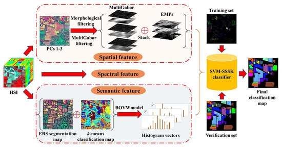
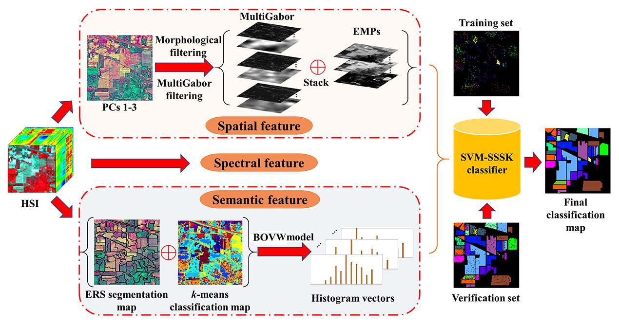
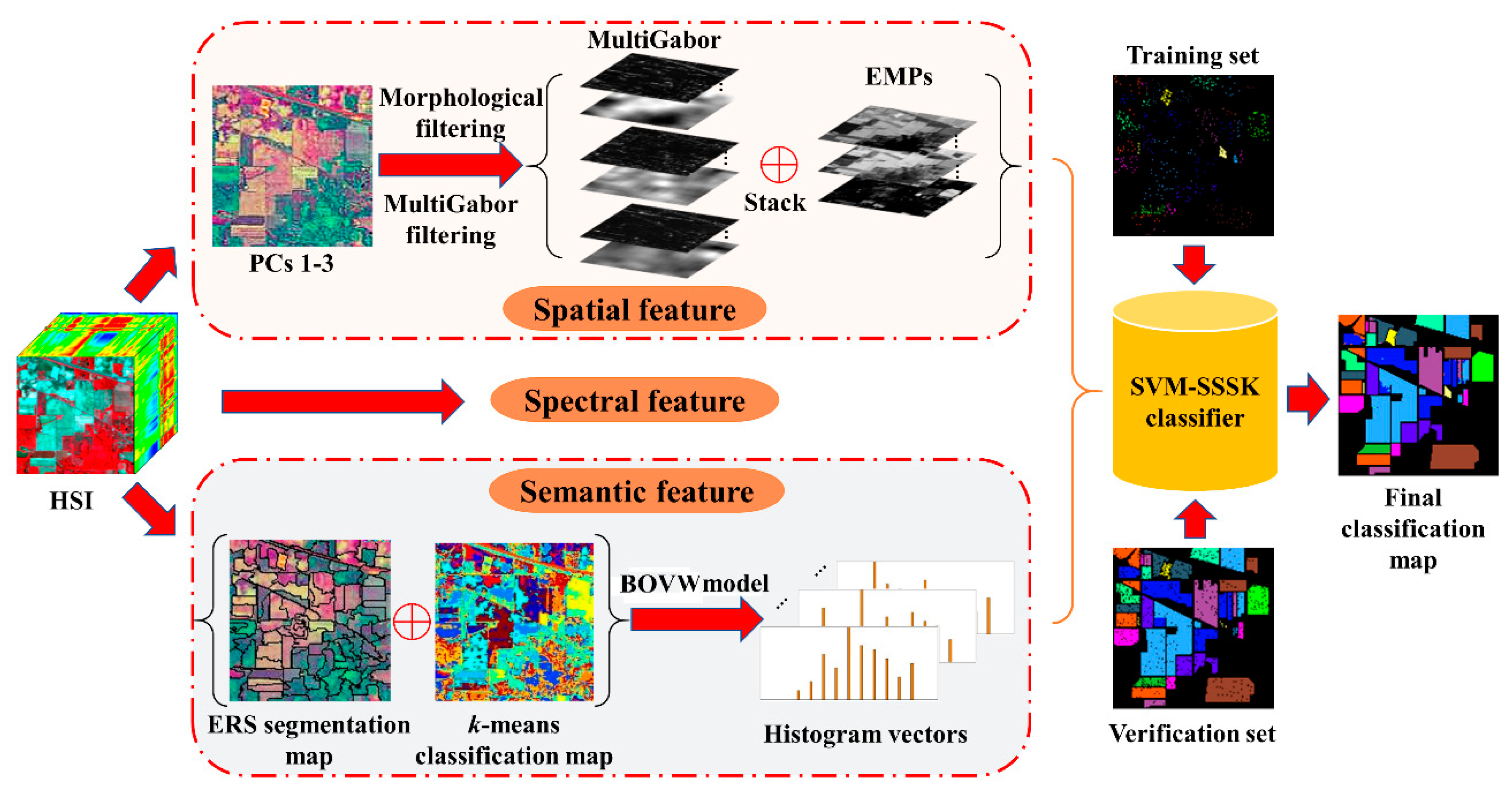
In this work, we present an SVM classifier with the spectral, spatial, and semantic kernels method (SVM-SSSK) for HSI classification. First, a PCA transform is performed on the original HSI to obtain the first three principle components (PCs 1–3). Then, the PCs 1–3 are used to obtain the EMP, Gabor features, and an ERS segmentation map. Next, to model the spatial information, the EMP and the Gabor features are combined to construct a new feature map, where each pixel is a stacked feature vector composed of structure and texture features. To ensure the uniform spatial characteristics, mean filtering is performed within each superpixel. Thereafter, to model the semantic information, a k-means clustering map and the ERS segmentation map are integrated to produce a feature vector for each superpixel. In the following, three single kernels are constructed to represent spectral, spatial, and semantic information, respectively, and a composite kernel function is defined as the weighted sum of the three kernel functions. Finally, the final classification map is obtained by using the SVM classifier with the composite kernel. The flowchart of the proposed method is illustrated in Figure 1.

3.1. Spatial Feature Extraction

To completely represent the spatial information, texture and structure features are directly combined for each pixel as a stacked vector. To this end, we use the EMP as the structure features of HSIs. The Gabor filter has been widely used for feature extraction for grayscale images and many studies have been proposed to extract the Gabor features from the first PC of HSIs. However, the texture information of some ground objects from PC 1 may not be sufficient to ensure there are better classification results. To avoid this problem, we performed the Gabor filtering on the PCs 1–3 in this work to extract the multiband Gabor (MultiGabor) features because these three PCs include over 99% of total variation in the image. A superpixel is usually defined as a uniform region in the image whose shape and size can be adaptive to different spatial structures. Nevertheless, each pixel corresponds to a stacked vector in the structure-texture feature image, which may be different from each other inside a superpixel. To ensure the uniform spatial features within each superpixel, the mean filtering is performed in each band of the structure-texture feature image. Eventually, the filtered spatial features are used for each pixel to construct the spatial kernel function.

3.2. Semantic Feature Extraction

Once the HSI has been segmented into nonoverlapping superpixels, each superpixel of the HSI can be considered as a separate image. Semantic features can represent similarities or differences between different superpixels. To extract the semantic features, the BOVW model was used in this work. Specifically, each superpixel can be regarded as a patch of an image in addition to being a document, and the spectral feature vector can also be used as a low-level feature. To group low-level features, the k-means clustering algorithm is used because of its simplicity, which indicates that the construction of a visual dictionary is an unsupervised process. Furthermore, it is more flexible to label the visual words since the number of the centers can be manually specified.

Once the visual word dictionary is constructed, the histogram information of visual words is used to describe the meaning of each superpixel. Specifically, the number of pixels inside each superpixel belonging to each cluster class is counted. Therefore, each superpixel can be represent by using a k × 1 histogram vector. In this way, the histogram vector of each superpixel can be used to represent semantic features. It should be noted that the pixels inside each superpixel should have the same semantic feature due to the homogeneity of the superpixel. The main procedures of semantic feature extraction are summarized in Algorithm 2.

Algorithm 2: Semantic Feature Extraction

Input: An original HSI u, the ERS segmentation map us consisting of N superpixels, the number of cluster centroids k.

Step 1: Perform the k-means algorithm to cluster u into k cluster centers.

Step 2: For i = 1, 2, …, N

(a) Count the number of pixels inside the ith superpixel belonging to each cluster. (b) Construct the k × 1 feature histogram vector as the semantic feature for the ith superpixel.

End

Step 3: Obtain the Semantic feature extraction map.

3.3. SVM-SSSK Method

So far, three different types of features have been obtained, namely, spectral, spatial and semantic. To fuse these features, the aforementioned composite kernel method was used to construct a novel HSI classification framework. Let $x_i\equiv \left\{x_i^{\mathrm{SPE}},x_i^{\mathrm{SPA}},x_i^{\mathrm{SEM}}\right\}$, so the composite kernel can be represented as follows:

$$K^{\mathrm{SPE-SPA-SEM}}\equiv K\left(x_i,x_j\right)=\langle \varphi \left(x_i\right),\varphi \left(x_j\right)\rangle$$

(19)

which can be defined through the weighted summation of the spectral, spatial, and semantic kernel functions as follows:

$$\begin{array}{c}{K}^{\mathrm{SPE-SPA-SEM}}\left(x_i,x_j\right)={\mu }^{\mathrm{SPE}}{K}^{\mathrm{SPE}}\left(x_i^{\mathrm{SPE}},x_j^{\mathrm{SPE}}\right)+{\mu }^{\mathrm{SPA}}{K}^{\mathrm{SPA}}\left(x_i^{\mathrm{SPA}},x_j^{\mathrm{SPA}}\right)+{\mu }^{\mathrm{SEM}}{K}^{\mathrm{SEM}}\left(x_i^{\mathrm{SEM}},x_j^{\mathrm{SEM}}\right)\\ s.t.,{\mu }^{\mathrm{SPE}}+{\mu }^{\mathrm{SPA}}+{\mu }^{\mathrm{SEM}}=1\end{array}$$

(20)

where ${\mu }^{\mathrm{SPE}}$, ${\mu }^{\mathrm{SPA}}$ and ${\mu }^{\mathrm{SEM}}$ are weights used to indicate the contribution of each piece of information involved in image classification. Let $\left\{x_1^{\mathrm{SPE}},x_2^{\mathrm{SPE}},\dots ,x_n^{\mathrm{SPE}}\right\}$, $\left\{x_1^{\mathrm{SPA}},x_2^{\mathrm{SPA}},\dots ,x_n^{\mathrm{SPA}}\right\}$ and $\left\{x_1^{\mathrm{SEM}},x_2^{\mathrm{SEM}},\dots ,x_n^{\mathrm{SEM}}\right\}$ be the spectral, spatial, and semantic features acquired from the training set $\left\{x_1,x_2,\dots ,x_n\right\}$. The widely used Gaussian RBF kernel was utilized to compute the kernel matrix for each piece of information. As described in Section 2.1, the spectral and spatial kernels are the same for (6) and (7) and the semantic function was defined as follows:

$$K^{\mathrm{SEM}}\left(x_i^{\mathrm{SEM}},x_j^{\mathrm{SEM}}\right)=\exp \left(-\gamma {\Vert x_i^{\mathrm{SEM}}-x_j^{\mathrm{SEM}}\Vert }^2\right).$$

(21)

The main procedures of the proposed algorithm are summarized in Algorithm 3.

Algorithm 3: SVM-SSSK

Input: An original HSI u, the available training/verification samples.

Step 1: Obtain PCs 1–3 of u;

Step 2: Perform the Gabor filtering on the PCs 1–3 to extract the MultiGabor features.

Step 3: Build the EMP by computing the MPs for the PCs 1–3 in Step 2 as described in Section 2.3.

Step 4: Conduct ERS as described in Section 2.4 obtain segmentation map with superpixels.

Step 5: Construct the spatial features as described in Section 3.1.

Step 6: Extract the semantic feature extraction by using Algorithm 1.

Step 7: Normalize u, the spatial feature, and semantic feature maps to (0,1).

Step 8: Construct the spectral, spatial, and semantic kernels as described in Section 3.3.

Step 9: Apply the SVM classifier with the proposed composite kernel in (20) to classify u using the training samples by choosing the optimized C and $\gamma$.

Step 10: Obtain the final classification map.

4. Experiment Results

4.1. Descriptions of Datasets

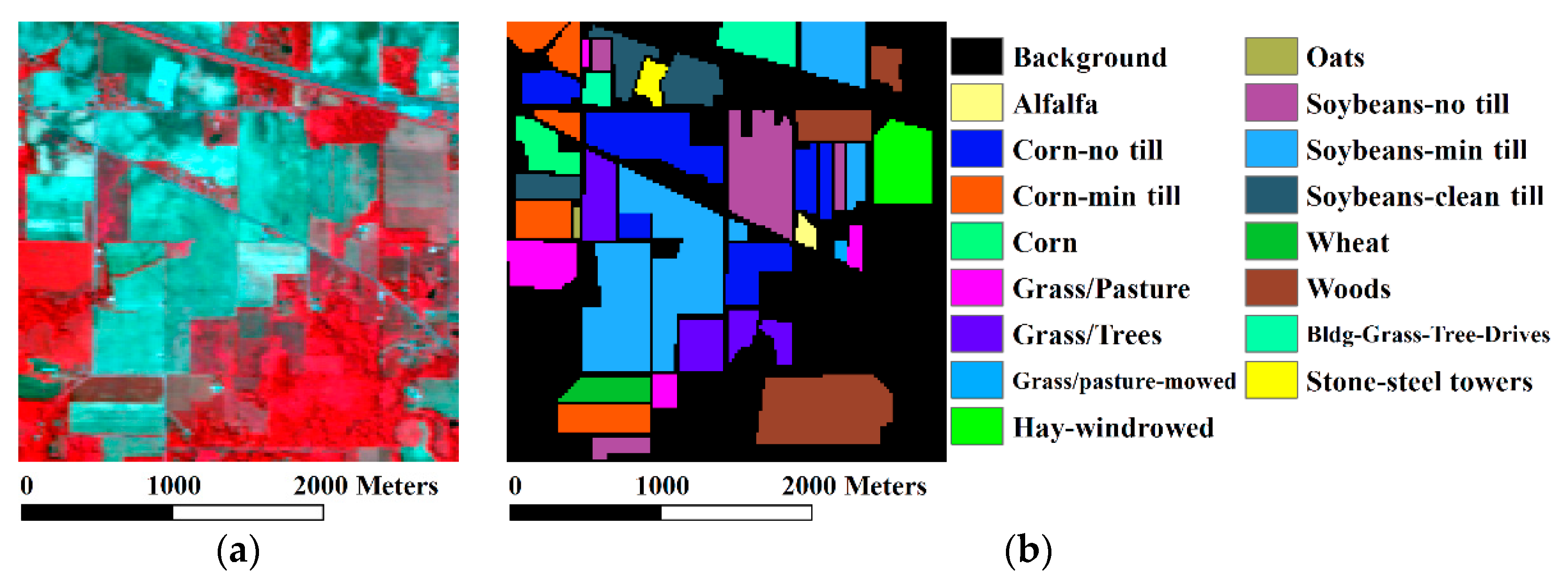
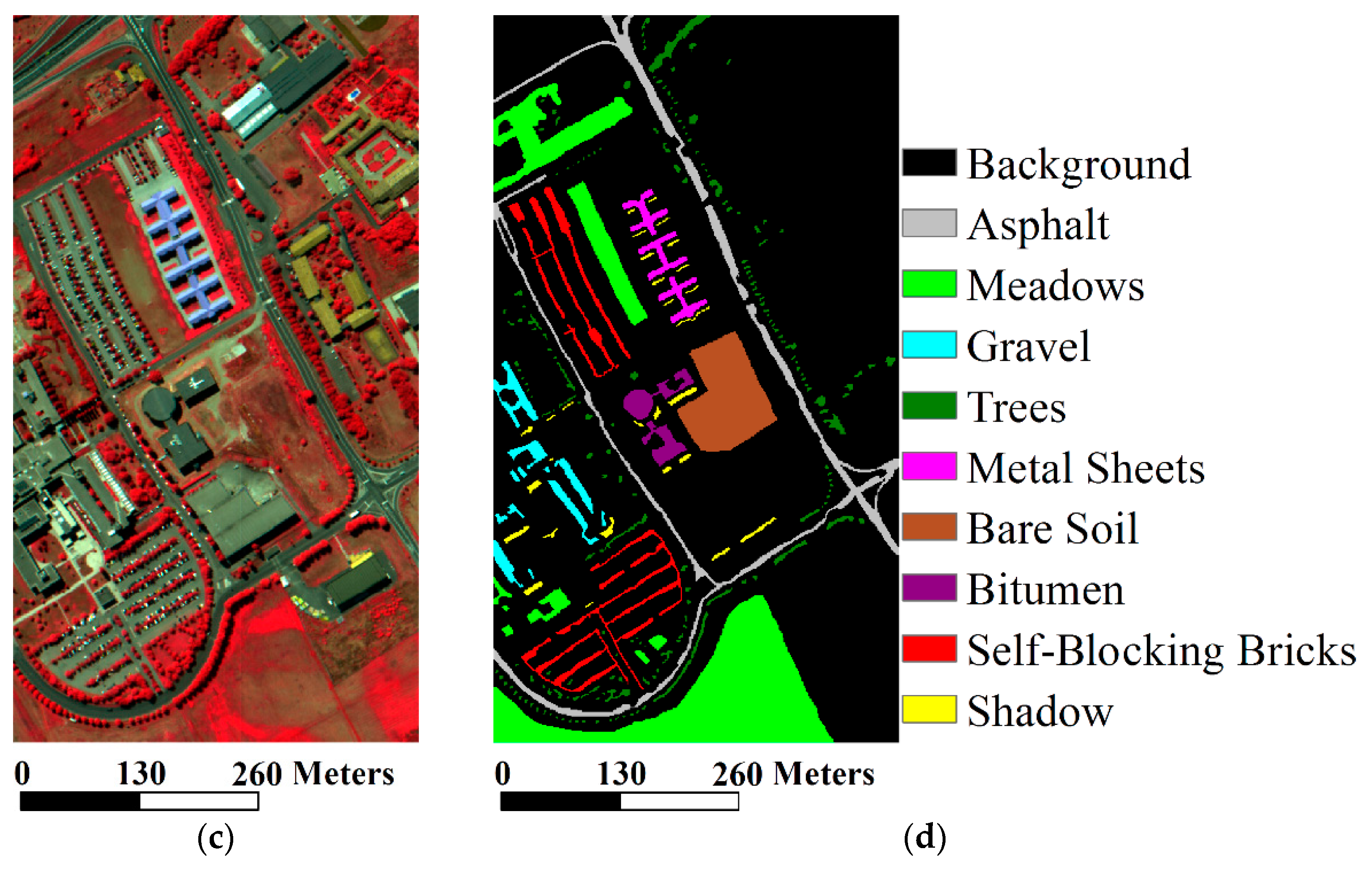
In order to validate the effectiveness of the proposed method, we reported some experiments on two widely used datasets of the Indian Pines and the University of Pavia. The AVIRIS Indian Pines image was covered with different agricultural/forest land covers and 16 groups were recorded in the ground truth data. The University of Pavia image was obtained over an urban area in Italy, consisting of nine typical urban structures in its ground truth data. The RGB false color and the corresponding ground truth data for the three datasets are illustrated in Figure 2. For the Indian Pines dataset, 10% of the known samples per class in the ground truth data were randomly selected as the training set and the rest of the known samples made up the validation set. If the training samples of a certain class was less than 10, then we fixed the number to 10. For the University of Pavia dataset, the same number of the known samples for each class were randomly chosen for training and the rest were for validation.

4.2. Experimental Setting

To verify the superiority of the proposed method, several kernel-based HSI classification methods were chosen for comparison, including three single kernel methods of SVM, EMP [30], and an edge-preserving filter (EPF) [17], two composite kernel methods of SVM-CK [27] and GCK [43], and two superpixel-based classification methods using spectral-spatial kernel (SC-SSK) [13] and multiple kernels (SC-MK) [46]. Moreover, we constructed a single kernel SVM classifier using both the spectral and texture information of each pixel for comparison, in which the texture information is represented using the MultiGabor features. For simplicity, we refer to this method as “MultiGabor”. The criteria of overall accuracy, average accuracy (average accuracy), kappa coefficient (κ), and the class-specific accuracy were used for quantitative evaluation. For objective comparison, we employed the optimized parameters for each method to obtain the optimal classification results, which can be comparable to that from the original references for the two datasets with the same number of training samples. In the following experiments, the parameters for each method are provided as follows:

(1)

For SVM, only the spectral features were used in the RBF kernel and such kernels were employed by all of the other methods, except for GCK. The optimal C and γ for each method were obtained by using five-fold cross validation with $C\in \left[2^{-5},2^{-4},\dots ,2^{15}\right]$ and $\gamma \in \left[2^{-15},2^{-14},\dots ,2^5\right]$, respectively.

(2)

The PCs 1–3 were used by the EMP, EPF, and MultiGabor methods for different purposes. Specifically, they were used for EMP to construct the MPs, which were computed using a flat disk-shaped structuring element with a radius from 1 to 11 with an interval of 2. Thus, EPF can form a guidance image with the following parameter settings: a 5 × 5 window for the bilateral filter, ${\delta }_s=3$, and ${\delta }_r=0.2$, and MultiGabor can construct the texture features with the following parameter settings: $N_s=4$, $N_d=6$, $U_h=0.49$, and $U_l=0.01$.

(3)

For SC-SSK, the parameters were fixed as $\mu =0.8$ and $\sigma =2$. The number of superpixels was fixed as 200 and 3000 for the Indian Pines and University of Pavia datasets, respectively.

(4)

For GCK, the spectral and spatial variances were fixed as ${\sigma }_{\mathrm{SPE}}=1.5$ and ${\sigma }_{\mathrm{SPA}}=2$, respectively, and $\lambda =10^{-5}$. The multinomial logistic regression classifier was used to obtain a probabilistic output in this method, instead of the SVMs.

(5)

For SVM-CK, the weight was fixed as $\mu =0.5$, and the EMP features were selected as the spatial information.

(6)

For SC-MK, the three weights were fixed as ${\mu }^{\mathrm{SPE}}=0.2$, ${\mu }^{\mathrm{Intras}}=0.4$ and ${\mu }^{\mathrm{Inters}}=0.4$, respectively, and the number of superpixels was fixed as 200.

(7)

For the SVM-SSSK, the number of the superpixels S was fixed as 100 and dimensionality of the semantic features D were fixed as 50 and 100 for the Indian Pines and University of Pavia datasets, respectively. The parameter settings for the construction of the spatial features were the same as that of the EMP and MultiGabor methods mentioned above. The three weights were fixed as ${\mu }^{\mathrm{SPE}}=0.2$, ${\mu }^{\mathrm{SPA}}=0.4$ and ${\mu }^{\mathrm{SEM}}=0.4$, respectively.

4.3. The Indian Pines Dataset

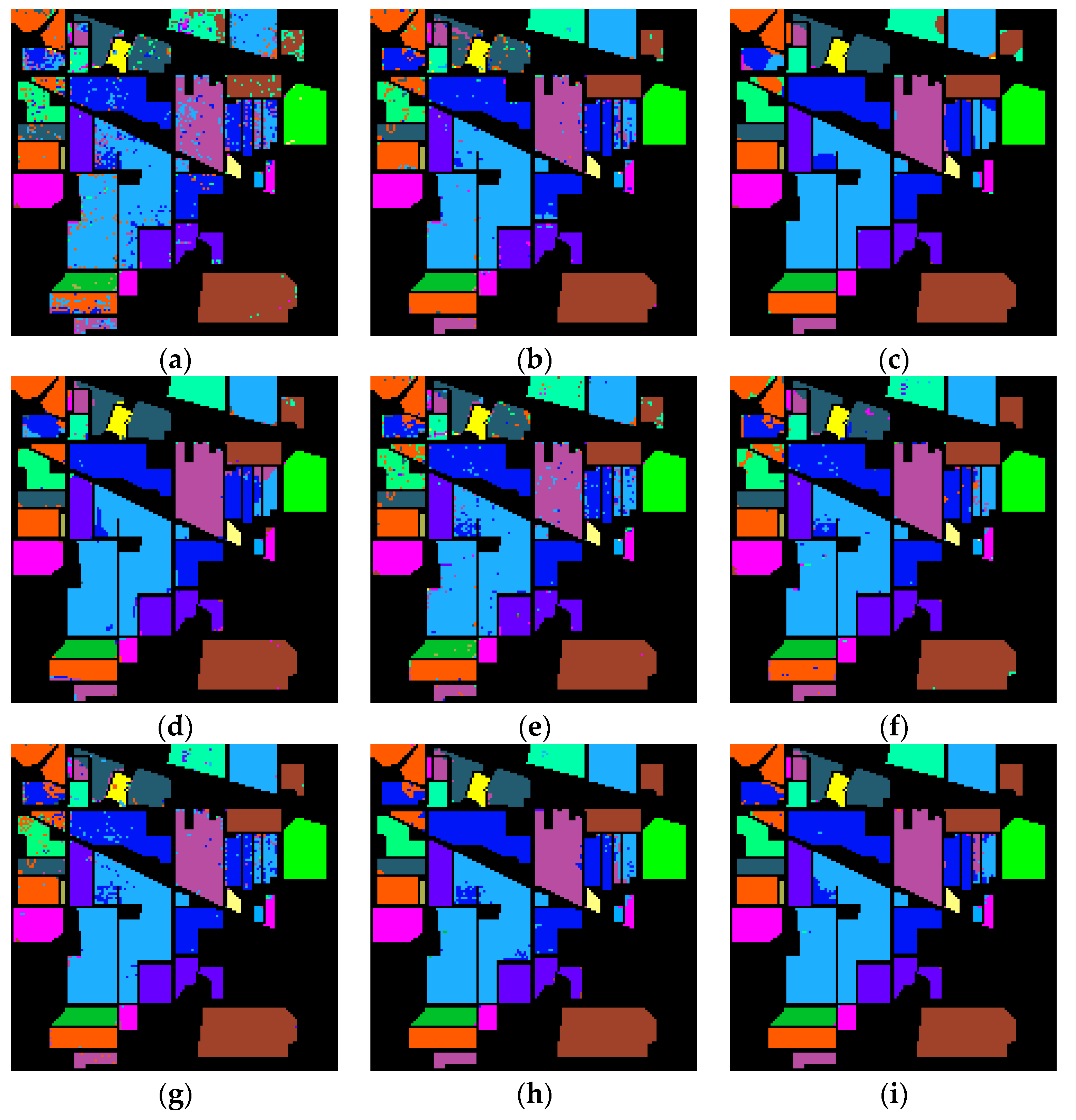
The classification results obtained by different methods are illustrated in Figure 3. The SVM classification result in Figure 3a was corrupted by a great deal of isolated class noise. The noise can be alleviated by the EMP, SVM-CK, SC-SSK, and GCK methods, but cannot be thoroughly removed by them, especially in the upper-left part of the figures, as shown in Figure 3b,e–g. The classification maps obtained by the rest of the methods were comparable and the noise effect was effectively minimized. However, some misclassification areas appeared in Figure 3c,d,h at the upper part of the image by the EPF, MultiGabor, and SC-MK methods. For instance, the boundaries of the image such as the Corn-no till in the upper left part of the image were contaminated with the class noise because the feature extraction in the EPF and MultiGabor methods was performed in a predefined sliding window in the image. Some classification errors involving the Soybeans-no till in the middle right part of the image cannot be effectively corrected by the SC-MK method. In comparison, the SVM-SSSK method can achieve a more homogenous classification map with smoother boundaries and nearly without any isolated noise in terms of visual inspection. As a result, only a few classification errors can be observed in Figure 3i.

The classification accuracies of this dataset are reported in

Table 1. The classification accuracies (%) of the Indian Pines dataset. The best accuracies for each row are marked in bold in each category.

	Training/Validation	SVM	EMP	EPF	MultiGabor	SVM-CK	SC-SSK	GCK	SC-MK	SVM-SSSK
overall accuracy	-	86.54 ± 0.79	94.15 ± 0.41	96.18 ± 0.98	95.63 ± 0.60	93.41 ± 0.91	96.40 ± 0.33	94.19 ± 0.26	96.90 ± 0.49	98.39 ± 0.17
average accuracy	-	87.52 ± 1.15	94.57 ± 0.55	94.65 ± 1.15	95.32 ± 1.44	93.75 ± 1.02	95.98 ± 0.30	94.19 ± 0.46	97.46 ± 0.40	98.30 ± 0.30
κ	-	84.63 ± 0.91	93.32 ± 0.47	95.63 ± 1.13	95.01 ± 0.69	92.49 ± 1.04	95.89 ± 0.38	93.36 ± 0.29	96.47 ± 0.55	98.16 ± 0.20
Alfalfa	10/36	87.22 ± 10.89	95.27 ± 1.34	92.78 ± 5.58	95.83 ± 3.53	95.27 ± 1.34	95.27 ± 1.34	95.27 ± 1.34	97.78 ± 1.17	97.78 ± 1.17
Corn-no till	142/1286	83.71 ± 1.44	88.72 ± 1.72	93.47 ± 3.58	92.22 ± 2.73	89.57 ± 2.41	94.05 ± 1.00	88.75 ± 1.50	94.33 ± 1.92	96.18 ± 1.40
Corn-min till	83/747	77.90 ± 4.97	94.38 ± 2.79	90.00 ± 9.03	95.30 ± 2.47	93.82 ± 1.75	93.92 ± 1.96	92.52 ± 1.89	97.24 ± 1.25	98.93 ± 0.84
Corn	23/214	76.08 ± 9.52	87.94 ± 5.91	98.41 ± 3.58	94.95 ± 3.32	80.66 ± 9.54	91.82 ± 2.25	86.64 ± 3.65	97.43 ± 1.11	95.56 ± 2.77
Grass/pasture	48/435	92.69 ± 2.33	92.41 ± 2.54	94.96 ± 1.34	92.99 ± 2.12	93.56 ± 1.95	94.64 ± 1.63	92.76 ± 2.30	96.09 ± 2.07	97.06 ± 1.93
Grass/trees	73/657	97.31 ± 1.22	97.09 ± 1.40	99.77 ± 0.11	96.20 ± 2.03	98.64 ± 0.61	99.62 ± 0.21	99.09 ± 0.59	99.56 ± 0.38	99.87 ± 0.11
Grass/pasture-mowed	10/18	92.78 ± 3.75	93.33 ± 5.74	75.56 ± 14.15	98.33 ± 2.69	93.89 ± 4.86	93.33 ± 4.38	96.11 ± 3.75	94.44 ± 5.24	96.11 ± 4.57
Hay-windrowed	47/431	98.59 ± 0.78	99.79 ± 0.17	99.98 ± 0.07	99.30 ± 0.71	99.86 ± 0.16	100 ± 0	99.93 ± 0.11	100 ± 0	100 ± 0
Overall accuracyts	10/10	98.00 ± 4.22	100 ± 0	95.00 ± 8.50	99.00 ± 3.16	99.00 ± 3.16	100 ± 0	100 ± 0	100 ± 0	100 ± 0
Soybeans-no till	97/875	81.06 ± 4.54	87.90 ± 2.78	93.29 ± 3.40	94.16 ± 2.19	87.18 ± 3.87	93.57 ± 1.27	87.42 ± 1.79	94.48 ± 1.84	97.47 ± 1.87
Soybeans-min till	245/2210	85.95 ± 1.34	96.64 ± 1.28	98.19 ± 1.15	97.36 ± 1.00	94.14 ± 1.21	97.64 ± 0.90	95.71 ± 1.21	96.09 ± 1.46	98.73 ± 0.81
Soybeans-clean till	59/534	86.25 ± 3.08	87.92 ± 3.40	99.18 ± 0.58	94.96 ± 1.60	90.80 ± 2.86	95.30 ± 1.30	94.42 ± 1.39	97.36 ± 1.41	98.84 ± 1.27
Wheat	20/185	96.65 ± 2.78	98.33 ± 0.47	99.62 ± 0.26	97.19 ± 1.22	97.08 ± 1.68	99.51 ± 0.17	99.46 ± 0.25	99.51 ± 0.17	99.68 ± 0.28
Woods	126/1139	95.49 ± 1.17	99.21 ± 0.60	99.52 ± 0.50	97.59 ± 1.31	98.46 ± 0.52	99.25 ± 0.32	99.77 ± 0.14	99.59 ± 0.41	99.61 ± 0.56
Bldg-Grass-Tree-Drives	38/348	60.83 ± 3.75	96.72 ± 1.82	86.15 ± 7.87	96.18 ± 3.34	92.21 ± 2.62	95.98 ± 1.72	96.21 ± 1.76	97.56 ± 1.58	98.88 ± 0.67
Stone-steel towers	10/83	89.76 ± 4.66	97.47 ± 1.20	98.56 ± 1.37	83.62 ± 13.56	95.91 ± 3.73	91.69 ± 3.66	83.01 ± 7.20	97.95 ± 0.81	98.07 ± 1.01

SVM: Support vector machine. EMP: extended morphological profile. EPF: edge-preserving filter. MultiGabor: multiband Gabor. SVM-CK: SVM with the composite kernel. SC-SSK: superpixel-based classification with the spectral-spatial kernel. GCK: generalized composite kernel. SC-MK: superpixel-based classification with multiple kernels. SVM-SSSK: SVM with the spectral, spatial, and semantic kernels.

for quantitative evaluation, which are the average results of the 10 times we conducted experiments using different training samples. Some observations can be found from this table as follows. First, the proposed method can obtain very good classification accuracies above 98.16% in terms of overall accuracy, average accuracy and κ, which are better than all the other methods. Second, the proposed method can achieve the highest class-specific accuracies for eleven classes. With the exceptions of Corn, Grass/pasture-mowed, Soybeans-clean till, and Woods and Stone-steel towers, all of the class-specific accuracies were obtained at 100%, including for two classes of Hay-windrowed and the overall accuracyts, validating the effectiveness of the proposed method for both large and tiny areas in the image. It is worth noting that the MultiGabor method can demonstrate better classification performance than the SVM, EMP, SVM-CK, and GCK methods in terms of visual inspection and classification accuracies, since the texture features for the agricultural covers are much more effective for describing the spatial structures of the Indian Pines dataset. Therefore, the texture information is significant for improving HSI classification and can be employed in the SVM-SSSK method as well.

In this work, McNemar’s test [53] was used to analyze the statistical significance of the proposed method with the other methods. This test has been commonly used in the field of remote sensing and is based upon the standardized normal test statistic:

$$Z=\frac{f_{12}-f_{21}}{\sqrt{f_{12}+f_{21}}}$$

(22)

where f₁₂ indicates the number of samples classified correctly by classifier 1 and incorrectly by classifier 2. The difference in accuracy between classifiers 1 and 2 is said to be statistically significant if |Z| > 1.96. The sign of Z indicates whether classifier 1 is more accurate than classifier 2 (Z > 0) or vice versa (Z < 0).

Table 2. Standardized normal test statistic (Z) for the Indian Pines dataset using 1041 training samples.

	SVM	EMP	EPF	MultiGabor	SVM−CK	SC−SSK	GCK	SC−MK	SVM−SSSK
SVM	−	−7.48	−10.14	−9.29	−6.77	−9.49	−7.25	−9.81	−12.01
EMP	7.48	−	−2.65	−1.84	0.70	−2.04	0.25	−2.31	−4.56
EPF	10.14	2.65	−	0.86	3.41	0.62	2.98	0.33	−1.90
MultiGabor	9.29	1.84	−0.86	−	2.55	−0.23	2.09	−0.57	−2.75
SVM−CK	6.77	−0.7	−3.41	−2.55	−	−2.78	−0.44	−3.05	−5.31
SC−SSK	9.49	2.04	−0.62	0.23	2.78	−	2.38	−0.26	−2.53
GCK	7.25	−0.25	−2.98	−2.09	0.44	−2.38	−	−2.64	−4.85
SC−MK	9.81	2.31	−0.33	0.57	3.05	0.26	2.64	−	−2.18
SCM−SSSK	12.01	4.56	1.90	2.75	5.31	2.53	4.85	2.18	−

lists the statistical significance of the classification results obtained by different methods for the Indian Pines dataset using McNemar’s test. It can be observed that the Z values between the SVM-SSSK method and the other classification methods were in the range of 1.90–12.01, which means that the differences between the proposed method and the other methods are significant, except for EPF. In particular, the SVM-SSSK method demonstrated significant difference with |Z| > 4 against the state-of-the-art SVM, EMP, SVM-CK, and GCK methods.

4.4. The University of Pavia Dataset

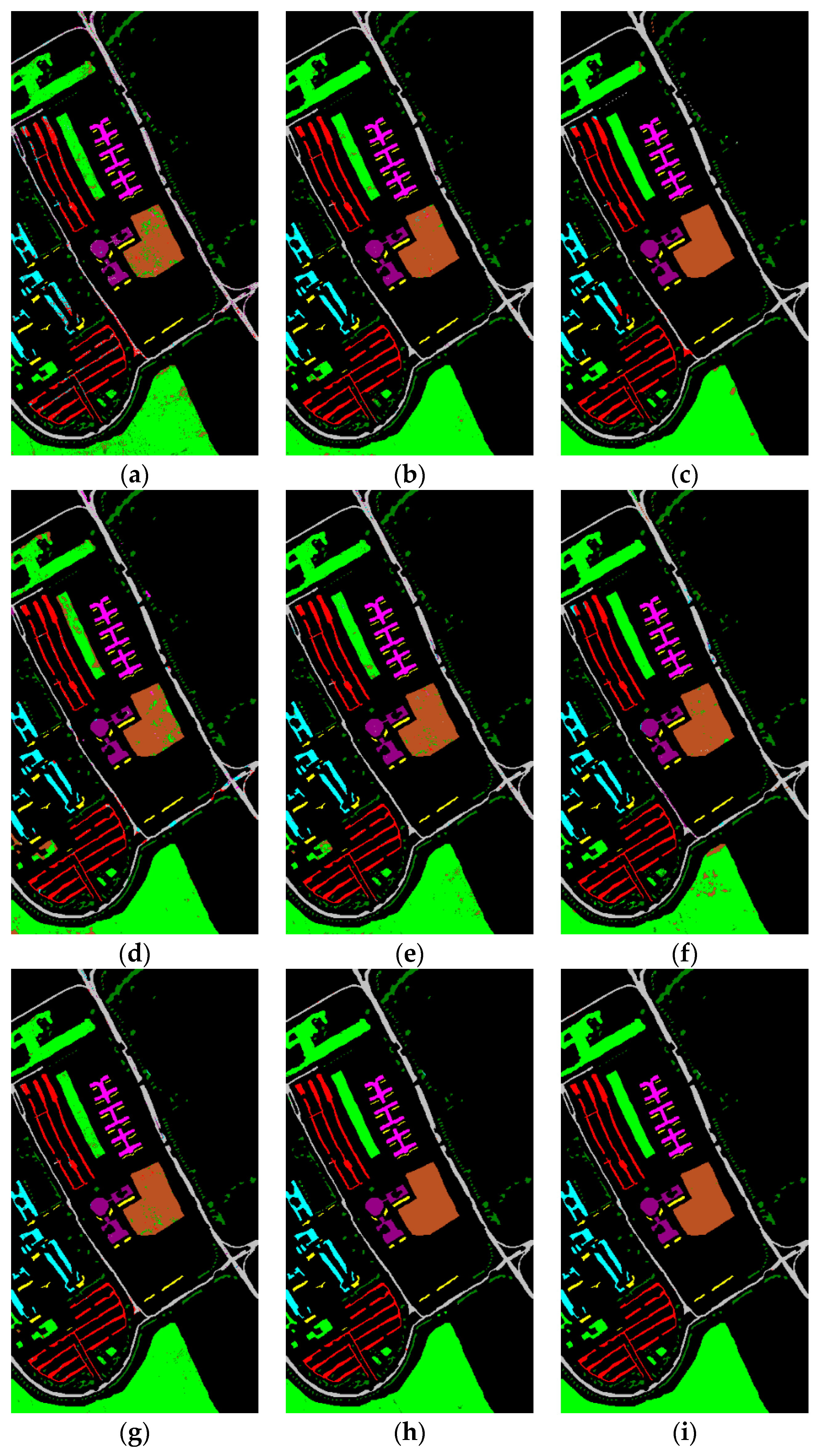
The classification maps produced by all the methods are shown in Figure 4. We can observe that there was a great deal of noise in the SVM map in Figure 4a. Although the noise effect can be reduced by the other methods, there was still isolated noise in the EMP, MultiGabor, SVM-CK, SC-SSK, and GCK maps in Figure 4b,d–g, respectively. For instance, the noise can be seen clearly in a large area belonging to Bare soil in the center of the previously mentioned maps. The noise was completely minimized by the EPF, SC-MK, and SVM-SSSK methods, as shown in Figure 4c,h,i, respectively. However, the classification errors were observed in a large area belonging to Meadows in the bottom of the EPF map, and other small areas in the left part of this map. The classification results of the SC-MK and SVM-SSSK methods are both quite good, but a few classification errors appeared in the aforementioned large area belonging to Meadows in the bottom of the image and the Self-blocking bricks in the middle of the image for the SC-MK method. In contrast, the SVM-SSSK method can effectively avoid the noise and misclassification, and its result is very close to the ground truth data in Figure 4d.

The classification accuracies of the University of Pavia dataset are reported in

Table 3. The classification accuracies (%) of the University of Pavia dataset. The best accuracies for each row are marked in bold in each category.

	Training/Validation	SVM	EMP	EPF	MultiGabor	SVM-CK	SC-SSK	GCK	SC-MK	SVM-SSSK
overall accuracy	-	90.71 ± 0.64	98.11 ± 0.51	97.98 ± 0.51	93.57 ± 0.48	97.36 ± 0.70	96.89 ± 0.39	98.31 ± 0.33	98.74 ± 0.35	99.77 ± 0.14
average accuracy	-	92.24 ± 0.23	98.90 ± 0.16	97.81 ± 0.34	96.32 ± 0.18	98.44 ± 0.41	97.85 ± 0.17	98.75 ± 0.14	99.20 ± 0.20	99.80 ± 0.10
Κ	-	87.69 ± 0.80	97.46 ± 0.68	97.28 ± 0.68	91.48 ± 0.61	96.47 ± 0.93	95.85 ± 0.51	97.73 ± 0.45	98.31 ± 0.47	99.69 ± 0.19
Asphalt	200/6431	86.36 ± 1.69	98.87 ± 0.54	98.02 ± 0.95	93.19 ± 0.89	97.94 ± 0.72	95.32 ± 0.41	98.29 ± 0.57	98.54 ± 0.63	99.15 ± 0.92
Meadows	200/18449	91.39 ± 1.50	97.24 ± 1.23	98.32 ± 0.91	91.17 ± 1.29	96.31 ± 1.26	96.46 ± 0.97	98.25 ± 0.72	98.39 ± 0.71	99.93 ± 0.04
Gravel	200/1899	84.03 ± 1.90	99.12 ± 0.25	92.12 ± 2.11	96.28 ± 0.72	98.31 ± 0.91	98.32 ± 0.48	99.12 ± 0.26	99.38 ± 0.69	99.90 ± 0.05
Trees	200/2864	96.28 ± 0.88	98.86 ± 0.63	94.69 ± 1.66	99.00 ± 0.65	99.11 ± 0.60	96.79 ± 1.01	99.08 ± 0.29	98.27 ± 0.57	99.74 ± 0.23
Metal sheets	200/1145	99.55 ± 0.16	99.86 ± 0.11	99.97 ± 0.06	100 ± 0	99.79 ± 0.12	99.71 ± 0.15	99.69 ± 0.24	99.99 ± 0.03	100 ± 0
Bare soil	200/4829	91.74 ± 1.31	98.16 ± 1.03	100 ± 0	92.79 ± 1.70	97.13 ± 0.84	98.25 ± 0.56	97.05 ± 0.51	99.88 ± 0.09	99.95 ± 0.09
Bitumen	200/1130	94.02 ± 1.46	99.42 ± 0.27	99.83 ± 0.33	98.01 ± 1.18	99.10 ± 0.41	98.41 ± 0.36	99.18 ± 0.38	99.98 ± 0.04	99.93 ± 0.04
Self-blocking bricks	200/3482	86.84 ± 1.74	98.65 ± 0.38	97.51 ± 1.57	97.43 ± 0.89	98.26 ± 0.74	97.46 ± 0.94	98.34 ± 0.62	98.40 ± 0.97	99.56 ± 0.36
Shadows	200/747	99.93 ± 0.12	99.94 ± 0.07	99.84 ± 0.14	99.01 ± 0.75	99.99 ± 0.04	99.97 ± 0.05	99.72 ± 0.16	99.99 ± 0.04	99.99 ± 0.04

for quantitative evaluation based on 10 experiments conducted using different training samples. First, we can observe that the highest overall accuracy, average accuracy and κ were reached by using the proposed method. Second, the proposed method achieved the highest class-specific accuracies for all the classes, except for Bitumen. Finally, the EMP, SVM-CK, GCK, and SVM-SSSK methods achieved very high classification accuracies because the shape features can be successfully represented by using EMP because there are many typical urban features in this dataset.

Table 4. Standardized normal test statistic (Z) for the University of Pavia dataset using 1800 training samples.

	SVM	EMP	EPF	MultiGabor	SVM−CK	SC−SSK	GCK	SC−MK	SVM−SSSK
SVM	−	−11.64	−12.20	−3.32	−10.30	−10.14	−11.73	−11.83	−14.29
EMP	11.64	−	−0.60	8.39	1.34	1.41	−0.13	−0.23	−2.67
EPF	12.20	0.60	−	8.98	1.93	2.02	0.45	0.37	−2.07
MultiGabor	3.32	−8.39	−8.98	−	−7.09	−6.95	−8.52	−8.63	−11.09
SVM−CK	10.30	−1.34	−1.93	7.09	−	0.08	−1.45	−1.58	−4.01
SC−SSK	10.14	−1.41	−2.02	6.95	−0.08	−	−1.56	−1.65	−4.08
GCK	11.73	0.13	−0.45	8.52	1.45	1.56	−	−0.08	−2.53
SC−MK	11.83	0.23	−0.37	8.63	1.58	1.65	0.08	−	−2.45
SCM−SSSK	14.29	2.67	2.07	11.09	4.01	4.08	2.53	2.45	−

lists the statistical significance of the classification results obtained by different methods for the University of Pavia dataset using McNemar’s test. It can be seen that all the Z values between the SVM-SSSK method and the other methods were higher than 2, indicating that the difference between the proposed method and the other methods are significant.

Based on the previously mentioned experiments of the two datasets, some similar conclusions can be drawn from Figure 3 and Figure 4 and Table 1, Table 2 and Table 3. First, both the SC-MK and SVM-SSSK methods characterized with the multiple kernels were better than the SVM-CK, SC-SSK, and GCK methods characterized with the spatial and spectral kernels in terms of both the visual effect and the classification accuracies, due to the fact that more information that is integrated into the kernel functions is capable of improving the classification performance. Second, the SVM-SSSK method can achieve more accurate classification accuracies than the SC-MK method. The multiple kernels of the SC-MK method are mainly constructed using both the spectral and spatial features of HSIs, whereas the proposed multiple kernels are defined using the spectral, spatial, and semantic features.

5. Discussion

In this section, the sensitivity of the parameters in the SVM-SSSK method is analyzed. Our experiments reported that the number of the superpixels S, the dimensionality of the semantic features D, and the weights in the spectral-spatial-semantic kernel greatly influence the performance of the proposed method. Furthermore, the sensitivity analysis of different training sets for all the methods is provided. In the following experiments, the training-validation sets for each dataset and the default parameter settings of the SVM-SSSK method were the same as those in Section 4.3 and Section 4.4.

5.1. Influence of S

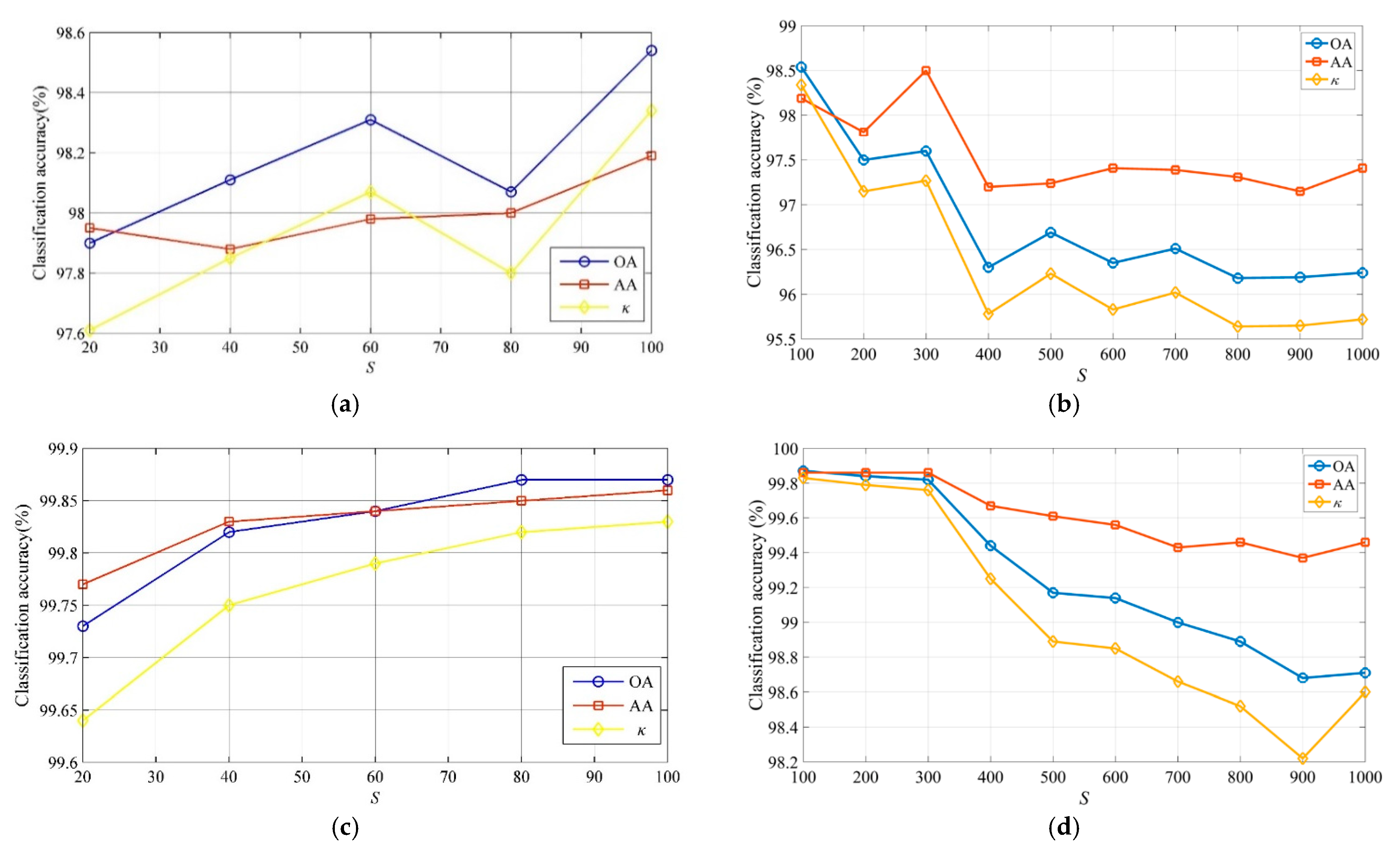
As mentioned in Section 2.4, a different number of superpixels can be obtained by the ERS algorithm, which may influence the region homogeneity and the semantic features. In the first experiment, we performed the proposed method to analyze the impact of S on classification performance. Figure 5 shows the overall accuracy, average accuracy and κ for the two datasets obtained by the SVM-SSSK method with the number of superpixels ranging from 20 to 100 with a step size of 10 or ranging from 100 to 1000 with a step size of 100. It can be observed that the classification accuracies of the two datasets mainly demonstrate an upward trend as S is increased from 20 to 100, and a downward trend as S is increased from 100 to 1000. In fact, when S is small, the image is divided into large areas by the ERS algorithm and the semantic features are not fully extracted. However when S is larger, the image is divided into more small-scale regions and the semantic features extracted from these regions may fluctuate from different regions belonging to the same class, meaning some miscellaneous components can be easily misclassified to other land covers. Consequently, the final classification accuracies are often decreased as the number of superpixels increased. If there is no prior knowledge, then we recommend choosing a relatively small value of S as S = 100 to ensure there are optimal classification results.

5.2. Influence of D

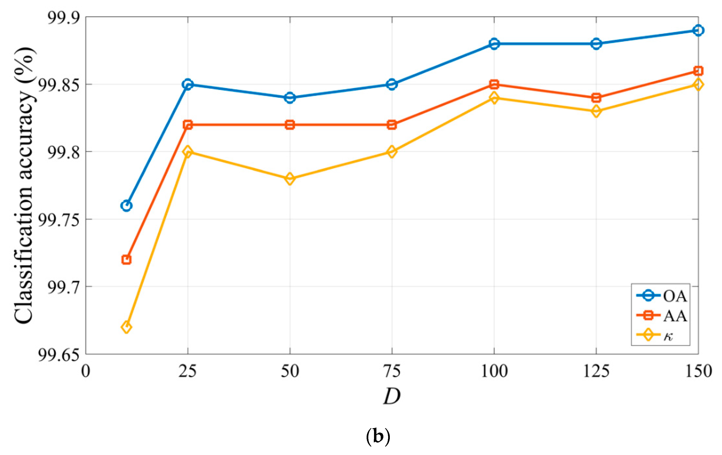
As described in Section 3.2, different dimensions of the semantic features can be obtained by modulating the number of the centroids in the k-means algorithm and can make a significant impact on the classification performance of the proposed method. In the second experiment, we performed the proposed method to analyze the impact of D on classification performance. Figure 6 shows the overall accuracy, average accuracy and κ for the two datasets obtained by the SVM-SSSK method with D ranging from 10 to 150. For the Indian Pines dataset, when D is increased from 10 to 50, the overall accuracy, average accuracy and κ rise very fast from 96.87%, 97.14%, and 96.42% to 98.58%, 98.21%, and 98.39%, respectively. When D is increased from 50 to 150, the classification accuracies remain steady. This means that more semantic information is used to improve the classification performance as D is increased. However, if D is very large, too more semantic features can easily cause information redundancy. For the University of Pavia dataset, as D is increased, the overall accuracy, average accuracy and κ generally show a slight rising trend. For instance, the overall accuracy, average accuracy and κ are increased by 0.13%, 0.14%, and 0.18% when D ranges from 10 to 150, respectively.

5.3. Impact of Weights

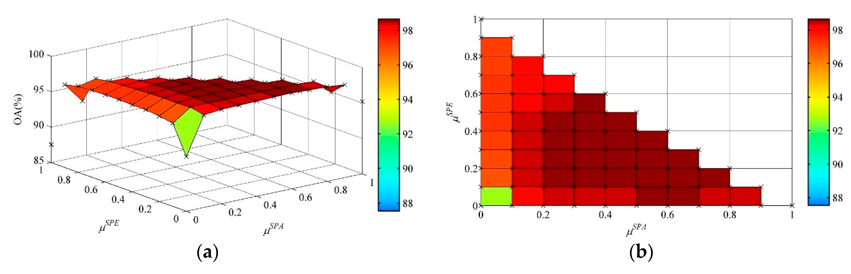
In the SVM-SSSK method, the weights in $K^{\mathrm{SPE-SPA-SEM}}$ can demonstrate the contribution of the spectral, spatial, and semantic information for classification. To uncover the interaction of the three weights in (20) on the classification performance, we analyzed different combinations of ${\mu }^{\mathrm{SPE}}$ and ${\mu }^{\mathrm{SPA}}$ in terms of overall accuracy according to the condition of ${\mu }^{\mathrm{SPE}}+{\mu }^{\mathrm{SPA}}+{\mu }^{\mathrm{SEM}}=1$. Figure 7 shows the 3-D plot and top view of the overall accuracy with the change of ${\mu }^{\mathrm{SPE}}$ and ${\mu }^{\mathrm{SPA}}$ from 0 to 1 with an interval of 0.1. The observations of this figure can be summarized as follows:

(1)

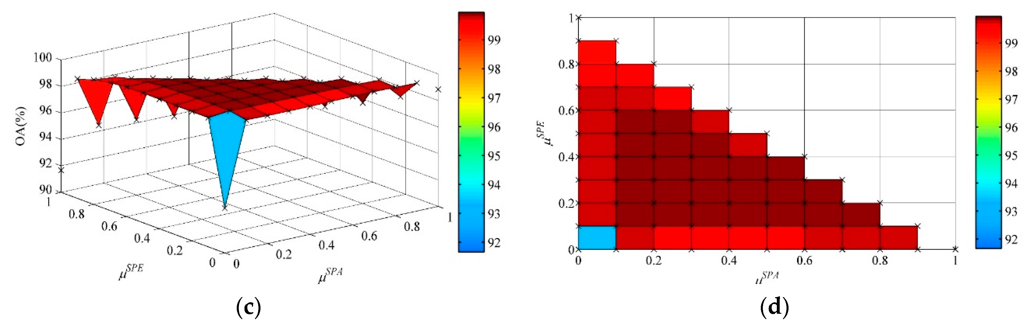
For the Indian Pines dataset, if the spectral, spatial, and semantic information was used separately, i.e., when ${\mu }^{\mathrm{SPE}}=1$ and ${\mu }^{\mathrm{SPA}}={\mu }^{\mathrm{SEM}}=0$, then the overall accuracy result was 87.54%; when ${\mu }^{\mathrm{SPA}}=1$ and ${\mu }^{\mathrm{SPE}}={\mu }^{\mathrm{SEM}}=0$, the overall accuracy result was 95.21%; when ${\mu }^{\mathrm{SEM}}=1$ and ${\mu }^{\mathrm{SPE}}={\mu }^{\mathrm{SPA}}=0$, the overall accuracy result was 92.71%. This means that the spatial and semantic information can be very useful supplements to the pixel-wise SVM classifier for improving classification accuracies. If we performed the SVM-SSSK method using both the spatial and semantic information, i.e., ${\mu }^{\mathrm{SPE}}=0$, $0<{\mu }^{\mathrm{SPA}}<1$, then the overall accuracy results were in the range of 98.07–98.56%; if we used both the spectral and semantic information, i.e., ${\mu }^{\mathrm{SPA}}=0$, $0<{\mu }^{\mathrm{SPE}}<1$, then the overall accuracy results were in the range of 96.68–97.34%; if we used both the spectral and spatial information, i.e., ${\mu }^{\mathrm{SEM}}=0$, $0<{\mu }^{\mathrm{SPA}}<1$, then the overall accuracy results were in the range of 93.86–96.38%. It can be observed that a significant decline in terms of overall accuracy occurred when using the proposed method without the sematic features. Based on the above analysis, the sematic features is capable of having a positive impact on classification accuracies. For the University of Pavia dataset: the lowest overall accuracy of 91.67% was achieved when ${\mu }^{\mathrm{SPE}}=1$ and ${\mu }^{\mathrm{SPA}}={\mu }^{\mathrm{SEM}}=0$; when ${\mu }^{\mathrm{SPA}}=1$, ${\mu }^{\mathrm{SPE}}={\mu }^{\mathrm{SEM}}=0$, the overall accuracy result was 98.85%; and when ${\mu }^{\mathrm{SEM}}=1$ and ${\mu }^{\mathrm{SPE}}={\mu }^{\mathrm{SPA}}=0$, the overall accuracy result was 93.38%. These observations show that the spatial and semantic features are more effective than the spectral features for further improving classification accuracies. Furthermore, when using the semantic features, i.e., ${\mu }^{\mathrm{SEM}}\ne 0$, overall accuracy results were achieved that were higher than 99%, whereas when ${\mu }^{\mathrm{SEM}}=0$, the overall accuracy results were in the range of 95.17–98.18%, which reflects a similar conclusion to for the Indian Pines dataset. In addition, for both two datasets, the overall accuracy results obtained by the proposed method when ${\mu }^{\mathrm{SPE}}\ne 0$, ${\mu }^{\mathrm{SPA}}\ne 0$ and ${\mu }^{\mathrm{SEM}}\ne 0$ were much better than that of the proposed method when only using the spectral information, which means that the inclusion of the semantic features can effectively improve the HSI classification accuracies.

(2)

The suitable selection of the weights can result in the highest overall accuracies. For instance, the highest overall accuracy for the Indian Pines and University of Pavia datasets was 98.66% when ${\mu }^{\mathrm{SPE}}=0.3$ and ${\mu }^{\mathrm{SPA}}=0.3$, and 99.95% when $0.2\le {\mu }^{\mathrm{SPE}}\le 0.4$ and ${\mu }^{\mathrm{SPA}}=0.1$, respectively. Finally, the SVM-SSSK method can achieve very stable classification results in most cases with different combinations of ${\mu }^{\mathrm{SPE}}$ and ${\mu }^{\mathrm{SPA}}$. There were a total of 66 combinations of these two weights used for parameter settings. Based on the statistics outlined in Figure 7, the overall accuracy result was better than 98% with the Indian Pines dataset for 42 of 66 (63.6%) cases, and all the overall accuracy results were higher than 99% for the University of Pavia dataset, except for the cases of ${\mu }^{\mathrm{SEM}}=0$ or ${\mu }^{\mathrm{SEM}}=1$.

To further verify the effectiveness of the semantic features, we performed McNemar’s tests for Indian Pines and University of Pavia datasets in five different situations: three for using one of the spectral, spatial, and semantic features alone and two for composite kernels of ${\mu }^{\mathrm{SPE}}=0.4$, ${\mu }^{\mathrm{SPA}}=0.6$, ${\mu }^{\mathrm{SEM}}=0$ (including the spectral and spatial features) and ${\mu }^{\mathrm{SPE}}=0.2$, ${\mu }^{\mathrm{SPA}}=0.4$, ${\mu }^{\mathrm{SEM}}=0.4$ (including the spectral, spatial, and semantic features).

Table 5. Standardized normal test statistic (Z) for the Indian Pines dataset using different features.

Features	${\mathit{\mu }}^{\mathbf{SPE}}$	${\mathit{\mu }}^{\mathbf{SPA}}$	${\mathit{\mu }}^{\mathbf{SEM}}$	${\mathit{\mu }}^{\mathbf{SPE}}\mathbf{+}{\mathit{\mu }}^{\mathbf{SPA}}$	${\mathit{\mu }}^{\mathbf{SPE}}\mathbf{+}{\mathit{\mu }}^{\mathbf{SPA}}\mathbf{+}{\mathit{\mu }}^{\mathbf{SEM}}$
${\mu }^{\mathrm{SPE}}$	-	−8.44	−4.98	−9.76	−12.13
${\mu }^{\mathrm{SPA}}$	8.44	−	3.45	−1.28	−3.64
${\mu }^{\mathrm{SEM}}$	4.98	−3.45	−	−4.80	−7.19
${\mu }^{\mathrm{SPE}}+{\mu }^{\mathrm{SPA}}$	9.76	1.28	4.80	−	−2.35
${\mu }^{\mathrm{SPE}}+{\mu }^{\mathrm{SPA}}+{\mu }^{\mathrm{SEM}}$	12.13	3.64	7.19	2.35	−

and

Table 6. Standardized normal test statistic (Z) for the Indian Pines dataset using different features.

Features	${\mathit{\mu }}^{\mathbf{SPE}}$	${\mathit{\mu }}^{\mathbf{SPA}}$	${\mathit{\mu }}^{\mathbf{SEM}}$	${\mathit{\mu }}^{\mathbf{SPE}}\mathbf{+}{\mathit{\mu }}^{\mathbf{SPA}}$	${\mathit{\mu }}^{\mathbf{SPE}}\mathbf{+}{\mathit{\mu }}^{\mathbf{SPA}}\mathbf{+}{\mathit{\mu }}^{\mathbf{SEM}}$
${\mu }^{\mathrm{SPE}}$	-	−7.57	−3.77	−10.32	−14.29
${\mu }^{\mathrm{SPA}}$	7.57	−	3.74	−2.88	−6.85
${\mu }^{\mathrm{SEM}}$	3.77	−3.74	−	−6.55	−10.60
${\mu }^{\mathrm{SPE}}+{\mu }^{\mathrm{SPA}}$	10.32	2.88	6.55	−	−4.01
${\mu }^{\mathrm{SPE}}+{\mu }^{\mathrm{SPA}}+{\mu }^{\mathrm{SEM}}$	14.29	6.85	10.60	4.01	−

list the statistical significance of the classification results obtained by the SVM-SSSK method using different types of the features for the Indian Pines and University of Pavia datasets using the McNemar’s test, respectively. We can observe that the Z values between the SVM-SSSK method using all the features and using any one or two types of the features were in the range of 2.35–12.13 and 4.01–14.29 for the Indian Pines and University of Pavia datasets, respectively, which validated that the classification results were greatly improved when using the semantic features. Therefore, the integration of the spectral, spatial, and semantic information is an effective way to obtain better classification results than using a single or double kernels when using the SVM classifier.

5.4. Sensitivity to Different Training Sets

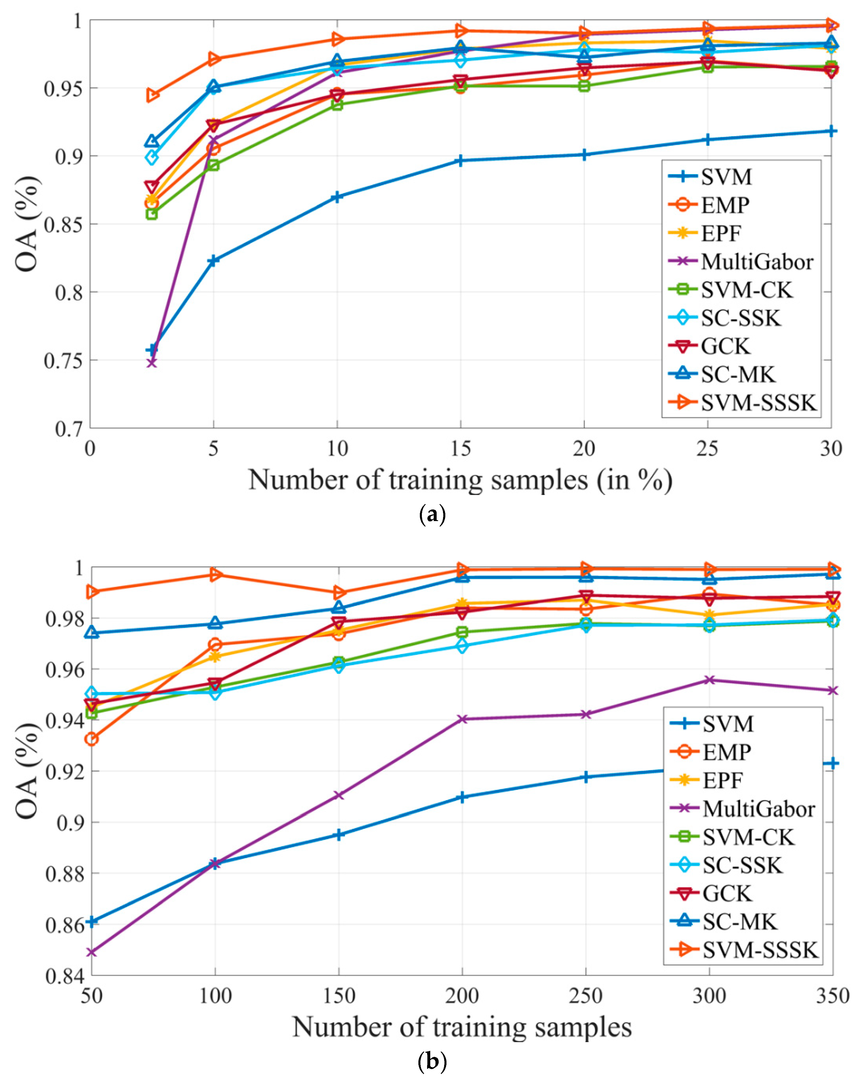
In this section, the sensitivity of the proposed method with respect to different training samples is analyzed. In this experiment, all the classification methods described in Section 4.2 were employed for comparison for the two datasets and the parameter settings were consistent with those in Section 4.3 and Section 4.4. For Indian Pines, different proportions ranging from 2.5% to 30% of the ground truth data were randomly selected for each class as training samples. In particular, the number of the training samples were fixed to 10 per class for some minority classes under the different cases. For University of Pavia, different numbers of known samples varying from 50 to 350 with a step size of 50 were randomly selected for each class as training samples. Figure 8 plots the impact of different training samples on overall accuracy for the two datasets. In this figure, the overall accuracy results achieved by all the methods are positively related to the number of training samples. For the Indian Pines dataset, the SVM-SSSK method can achieve the best overall accuracy results with respect to different training sets. In particular, the SVM-SSSK method outperformed the other methods when the number of the training samples is very limited. For instance, an overall accuracy of 94.47% was obtained by the proposed method, which is 3.46–19.7% higher than the other methods when the proportion of the number of training samples is only 2.5%. Furthermore, when the proportion was more than 20%, the overall accuracy results of the MultiGabor and SVM-SSSK methods were comparable, indicating that the texture information is important for representing the spatial features for this dataset. For the University of Pavia dataset, the SVM-SSSK method was obviously superior to the other methods under all of the cases. Specifically, the SVM-SSSK method can obtain an overall accuracy of 99.03% when the number of training samples is only 50 per class and this overall accuracy result is better than that of all the other methods under different training sets, except for the SC-MK method when the number of training samples is more than 200 per class. Meanwhile, the overall accuracy achieved by the SVM-SSSK method was stable around the remarkable 99.9% level when the number of training samples is more than 150 per class. Based on the above observations, the proposed method is capable of achieving better classification accuracies for different HSIs than the other methods.

6. Conclusions

In this paper, we propose an HSI classification method by combining spectral, spatial and semantic information into an SVM classifier using multiple kernels. Specifically, the spectral kernel is defined using spectral features, the spatial kernel is constructed by stacking the structure and texture information of each pixel, and the semantic kernel is developed by performing the BOVW algorithm within each superpixel of the image. The main advantages of the proposed method are twofold: first, semantic information is an important supplement in addition to the commonly used spectral and spatial information. Second, additional information integrated into the kernel function can improve classification performance. The experimental results on two hyperspectral datasets confirm the following conclusions: (1) The combination of spectral, spatial and semantic features in the SVM-SSSK method can effectively improve classification accuracy. For instance, the overall accuracy values by the SVM-SSSK method when ${\mu }^{\mathrm{SPE}}+{\mu }^{\mathrm{SPA}}<1$ were much higher than that when ${\mu }^{\mathrm{SEM}}=0$. (2) The SVM-SSSK method can produce more accurate classification results than all kernel-based HSI classification methods mentioned in Section 4.2, even with limited training samples. For example, our method improves the overall accuracy for the Indian Pines dataset by 3.46–19.7% when the proportion of the ground truth data per class is 2.5%, as well as 1.62–14.12% higher accuracy for the University of Pavia dataset with 50 training samples for each class. (3) The SVM- SSSK method can use different weights for the three kernels in most cases to achieve stable classification accuracy. In short, SVM-SSSK can be used as a very promising multiple kernel learning technique for HSI classification. Future work mainly includes developing more effective learning methods to integrate features in HSIs.

References

- Haboudane, D.; Miller, J.R.; Pattey, E.; Zarco-Tejada, P.J.; Strachan, I.B. Hyperspectral vegetation indices and novel algorithms for predicting green LAI of crop canopies: Modeling and validation in the context of precision agriculture. Remote Sens. Environ. 2004, 90, 337–352. [Google Scholar] [CrossRef]
- Stein, D.W.J.; Beaven, S.G.; Hoff, L.E.; Winter, E.M.; Schaum, A.P.; Stocker, A.D. Anomaly detection from hyperspectral imagery. IEEE Signal Process. Mag. 2002, 19, 58–69. [Google Scholar] [CrossRef] [Green Version]
- Zarco-Tejada, P.J.; Miller, J.R.; Mohammed, G.H.; Noland, T.L.; Sampson, P.H. Vegetation stress detection through chlorophyll a+b estimation and fluorescence effects on hyperspectral imagery. J. Environ. Qual. 2002, 31, 1433–1441. [Google Scholar] [CrossRef] [PubMed]
- Camps-Valls, G.; Bruzzone, L. Kernel-based methods for hyperspectral image classification. IEEE Trans. Geosci. Remote Sens. 2005, 43, 1351–1362. [Google Scholar] [CrossRef]
- Melgani, F.; Bruzzone, L. Classification of hyperspectral remote sensing images with support vector machines. IEEE Trans. Geosci. Remote Sens. 2004, 42, 1778–1790. [Google Scholar] [CrossRef] [Green Version]
- Cortes, C.; Vapnik, V. Support vector machine. Mach. Learn. 1995, 20, 273–297. [Google Scholar] [CrossRef]
- Böhning, D. Multinomial logistic regression algorithm. Ann. Inst. Stat. Math. 1992, 44, 197–200. [Google Scholar] [CrossRef]
- Li, J.; Bioucas-Dias, J.M.; Plaza, A. Semisupervised hyperspectral image segmentation using multinomial logistic regression with active learning. IEEE Trans. Geosci. Remote Sens. 2010, 48, 4085–4098. [Google Scholar] [CrossRef] [Green Version]
- Li, J.; Bioucas-Dias, J.M.; Plaza, A. Spectral-spatial hyperspectral image segmentation using subspace multinomial logistic regression and Markov random fields. IEEE Trans. Geosci. Remote Sens. 2012, 50, 809–823. [Google Scholar] [CrossRef]
- Tarabalka, Y.; Chanussot, J. Spectral-Spatial Classification of Hyperspectral Imagery Based on Partitional Clustering Techniques. IEEE Trans. Geosci. Remote Sens. 2009, 47, 2973–2987. [Google Scholar] [CrossRef]
- Camps-Valls, G.; Shervashidze, N.; Borgwardt, K.M. Spatio-spectral remote sensing image classification with graph kernels. IEEE Geosci. Remote Sens. Lett. 2010, 7, 741–745. [Google Scholar] [CrossRef]
- Bernard, K.; Tarabalka, Y.; Angulo, J.; Chanussot, J.; Benediktsson, J.A. Spectral-Spatial Classification of Hyperspectral Data Based on a Stochastic Minimum Spanning Forest Approach. IEEE Trans. Image Process. 2012, 21, 2008–2021. [Google Scholar] [CrossRef] [PubMed] [Green Version]
- Mathieu, F.; Jocelyn, C.; Atli, B.J. A spatial–spectral kernel-based approach for the classification of remote-sensing images. Pattern Recognit. 2012, 45, 381–392. [Google Scholar]
- Li, J.; Bioucas-Dias, J.M.; Plaza, A. Spectral-Spatial Classification of Hyperspectral Data Using Loopy Belief Propagation and Active Learning. IEEE Trans. Geosci. Remote Sens. 2013, 51, 844–856. [Google Scholar] [CrossRef]
- Fang, L.; Li, S.; Kang, X.; Benediktsson, J.A. Spectral-Spatial Hyperspectral Image Classification via Multiscale Adaptive Sparse Representation. IEEE Trans. Geosci. Remote Sens. 2014, 52, 7738–7749. [Google Scholar] [CrossRef]
- Ghamisi, P.; Benediktsson, J.A.; Ulfarsson, M.O. Spectral-Spatial Classification of Hyperspectral Images Based on Hidden Markov Random Fields. IEEE Trans. Geosci. Remote Sens. 2014, 52, 2565–2574. [Google Scholar] [CrossRef] [Green Version]
- Kang, X.; Li, S.; Benediktsson, J.A. Spectral-Spatial Hyperspectral Image Classification With Edge-Preserving Filtering. IEEE Trans. Geosci. Remote Sens. 2014, 52, 2666–2677. [Google Scholar] [CrossRef]
- Khodadadzadeh, M.; Li, J.; Plaza, A.; Ghassemian, H.; Bioucas-Dias, J.M.; Li, X. Spectral-Spatial Classification of Hyperspectral Data Using Local and Global Probabilities for Mixed Pixel Characterization. IEEE Trans. Geosci. Remote Sens. 2014, 52, 6298–6314. [Google Scholar] [CrossRef]
- Falco, N.; Benediktsson, J.A.; Bruzzone, L. Spectral and Spatial Classification of Hyperspectral Images Based on ICA and Reduced Morphological Attribute Profiles. IEEE Trans. Geosci. Remote Sens. 2015, 53, 6223–6240. [Google Scholar] [CrossRef] [Green Version]
- Fang, L.; Li, S.; Kang, X.; Benediktsson, J.A. Spectral-Spatial Classification of Hyperspectral Images With a Superpixel-Based Discriminative Sparse Model. IEEE Trans. Geosci. Remote Sens. 2015, 53, 4186–4201. [Google Scholar] [CrossRef]
- Jia, S.; Zhang, X.; Li, Q. Spectral-Spatial Hyperspectral Image Classification Using l1/2 Regularized Low-Rank Representation and Sparse Representation-Based Graph Cuts. IEEE J. Sel. Top. Appl. Earth Obs. Remote Sens. 2015, 8, 2473–2484. [Google Scholar] [CrossRef]
- Xia, J.; Chanussot, J.; Du, P.; He, X. Spectral-Spatial Classification for Hyperspectral Data Using Rotation Forests With Local Feature Extraction and Markov Random Fields. IEEE Trans. Geosci. Remote Sens. 2015, 53, 2532–2546. [Google Scholar] [CrossRef]
- Song, H.; Wang, Y. A Spectral-Spatial Classification of Hyperspectral Images Based on the Algebraic Multigrid Method and Hierarchical Segmentation Algorithm. Remote Sens. 2016, 8, 296. [Google Scholar] [CrossRef] [Green Version]
- Fauvel, M.; Tarabalka, Y.; Benediktsson, J.A.; Chanussot, J.; Tilton, J.C. Advances in Spectral-Spatial Classification of Hyperspectral Images. Proc. IEEE 2013, 101, 652–675. [Google Scholar] [CrossRef] [Green Version]
- Camps-Valls, G.; Tuia, D.; Bruzzone, L.; Benediktsson, J.A. Advances in Hyperspectral Image Classification: Earth monitoring with statistical learning methods. IEEE Signal Peocess. Mag. 2014, 31, 45–54. [Google Scholar] [CrossRef] [Green Version]
- He, L.; Li, J.; Liu, C.; Li, S. Recent Advances on Spectral-Spatial Hyperspectral Image Classification: An Overview and New Guidelines. IEEE Trans. Geosci. Remote Sens. 2018, 56, 1579–1597. [Google Scholar] [CrossRef]
- Camps-Valls, G.; Gomez-Chova, L.; Munoz-Mari, J.; Vila-Frances, J.; Calpe-Maravilla, J. Composite kernels for hyperspectral image classification. IEEE Geosci. Remote Sens. Lett. 2006, 3, 93–97. [Google Scholar] [CrossRef]
- Shen, L.; Zhu, Z.; Jia, S.; Zhu, J.; Sun, Y. Discriminative Gabor Feature Selection for Hyperspectral Image Classification. IEEE Geosci. Remote Sens. Lett. 2013, 10, 29–33. [Google Scholar] [CrossRef]
- Huang, X.; Zhang, L. A comparative study of spatial approaches for urban mapping using hyperspectral ROSIS images over PAVIA City, northern ITALY. Int. J. Remote Sens. 2009, 30, 3205–3221. [Google Scholar] [CrossRef]
- Benediktsson, J.A.; Palmason, J.A.; Sveinsson, J.R. Classification of Hyperspectral Data From Urban Areas Based on Extended Morphological Profiles. IEEE Trans. Geosci. Remote Sens. 2005, 43, 480–491. [Google Scholar] [CrossRef]
- Farag, A.A.; Mohamed, R.M.; El-Baz, A. A unified framework for MAP estimation in remote sensing image segmentation. IEEE Trans. Geosci. Remote Sens. 2005, 43, 1617–1634. [Google Scholar] [CrossRef]
- Tarabalka, Y.; Fauvel, M.; Chanussot, J.; Benediktsson, J.A. SVM-and MRF-based method for accurate classification of hyperspectral images. IEEE Geosci. Remote Sens. Lett. 2010, 7, 736–740. [Google Scholar] [CrossRef] [Green Version]
- Zhang, B.; Li, S.; Jia, X.; Gao, L.; Peng, M. Adaptive Markov Random Field Approach for Classification of Hyperspectral Imagery. IEEE Geosci. Remote Sens. Lett. 2011, 8, 973–977. [Google Scholar] [CrossRef]
- Moser, G.; Serpico, S.B. Combining Support Vector Machines and Markov Random Fields in an Integrated Framework for Contextual Image Classification. IEEE Trans. Geosci. Remote Sens. 2013, 51, 2734–2752. [Google Scholar] [CrossRef]
- Bai, J.; Xiang, S.; Pan, C. A Graph-Based Classification Method for Hyperspectral Images. IEEE Trans. Geosci. Remote Sens. 2013, 51, 803–817. [Google Scholar] [CrossRef]
- Golipour, M.; Ghassemian, H.; Mirzapour, F. Integrating hierarchical segmentation maps with MRF prior for classification of hyperspectral images in a Bayesian framework. IEEE Trans. Geosci. Remote Sens. 2016, 54, 805–816. [Google Scholar] [CrossRef]
- Blaschke, T. Object based image analysis for remote sensing. ISPRS J. Photogramm. Remote Sens. 2010, 65, 2–16. [Google Scholar] [CrossRef] [Green Version]
- Huang, X.; Zhang, L. An Adaptive Mean-Shift Analysis Approach for Object Extraction and Classification From Urban Hyperspectral Imagery. IEEE Trans. Geosci. Remote Sens. 2008, 46, 4173–4185. [Google Scholar] [CrossRef]
- Tarabalka, Y.; Chanussot, J.; Benediktsson, J.A. Segmentation and classification of hyperspectral images using watershed transformation. Pattern Recognit. 2010, 43, 2367–2379. [Google Scholar] [CrossRef] [Green Version]
- Tarabalka, Y.; Tilton, J.C.; Benediktsson, J.A.; Chanussot, J. A Marker-Based Approach for the Automated Selection of a Single Segmentation From a Hierarchical Set of Image Segmentations. IEEE J. Sel. Top. Appl. Earth Obs. Remote Sens. 2012, 5, 262–272. [Google Scholar] [CrossRef] [Green Version]
- Tarabalka, Y.; Chanussot, J.; Benediktsson, J.A. Segmentation and Classification of Hyperspectral Images Using Minimum Spanning Forest Grown From Automatically Selected Markers. IEEE Trans. Syst. Manand Cybern. Part B Cybern. 2010, 40, 1267–1279. [Google Scholar] [CrossRef] [PubMed] [Green Version]
- Wang, Y.; Song, H.; Zhang, Y. Spectral-Spatial Classification of Hyperspectral Images Using Joint Bilateral Filter and Graph Cut Based Model. Remote Sens. 2016, 8, 748. [Google Scholar] [CrossRef] [Green Version]
- Li, J.; Marpu, P.R.; Plaza, A.; Bioucas-Dias, J.M.; Benediktsson, J.A. Generalized Composite Kernel Framework for Hyperspectral Image Classification. IEEE Trans. Geosci. Remote Sens. 2013, 51, 4816–4829. [Google Scholar] [CrossRef]
- Wang, Y.; Duan, H. Classification of Hyperspectral Images by SVM Using a Composite Kernel by Employing Spectral, Spatial and Hierarchical Structure Information. Remote Sens. 2018, 10, 441. [Google Scholar] [CrossRef]
- Wang, Y.; Duan, H. Spectral–spatial classification of hyperspectral images by algebraic multigrid based multiscale information fusion. Int. J. Remote Sens. 2018, 40, 1301–1330. [Google Scholar] [CrossRef]
- Fang, L.; Li, S.; Duan, W.; Ren, J.; Benediktsson, J.A. Classification of Hyperspectral Images by Exploiting Spectral-Spatial Information of Superpixel via Multiple Kernels. IEEE Trans. Geosci. Remote Sens. 2015, 53, 6663–6674. [Google Scholar] [CrossRef] [Green Version]
- Wang, Y.; Zhang, Y.; Song, H. A Spectral-Texture Kernel-Based Classification Method for Hyperspectral Images. Remote Sens. 2016, 8, 919. [Google Scholar] [CrossRef] [Green Version]
- Xu, S.; Fang, T.; Li, D.; Wang, S. Object Classification of Aerial Images With Bag-of-Visual Words. IEEE Geosci. Remote Sens. Lett. 2010, 7, 366–370. [Google Scholar] [CrossRef]
- Huang, X.; Zhang, L.P. An SVM Ensemble Approach Combining Spectral, Structural, and Semantic Features for the Classification of High-Resolution Remotely Sensed Imagery. IEEE Trans. Geosci. Remote Sens. 2013, 51, 257–272. [Google Scholar] [CrossRef]
- Pesaresi, M.; Benediktsson, J.A. A new approach for the morphological segmentation of high-resolution satellite imagery. IEEE Trans. Geosci. Remote Sens. 2001, 39, 309–320. [Google Scholar] [CrossRef] [Green Version]
- Mirzapour, F.; Ghassemian, H. Using GLCM and Gabor Filters for Classification of PAN Images. In Proceedings of the 2013 21st Iranian Conference on Electrical Engineering, Mashhad, Iran, 14–16 May 2013. [Google Scholar]
- Liu, M.-Y.; Tuzel, O.; Ramalingam, S.; Chellappa, R. Entropy Rate Superpixel Segmentation. In Proceedings of the IEEE Conference on Computer Vision And Pattern Recognition, Colorado Springs, CO, USA, 20–25 June 2011. [Google Scholar]
- Foody, G.M. Thematic map comparison: Evaluating the statistical significance of differences in classification accuracy. Photogramm. Eng. Remote Sens. 2004, 70, 627–633. [Google Scholar] [CrossRef]
Figure 1.
Illustration of the proposed classification method for hyperspectral images.
Figure 2.
Hyperspectral images and the corresponding ground truth data. (a) RGB false color of the Indian Pines dataset with 47, 23, and 13 samples; (b) ground truth data of the Indian Pines dataset; (c) RGB false color of the University of Pavia dataset with 80, 50, and 30 samples; (d) ground truth data of the University of Pavia dataset.
Figure 3.
Classification maps for the Indian Pines dataset using different methods. (a) Support vector machine (SVM), (b) extended morphological profile (EMP), (c) edge-preserving filter (EPF), (d) multiband Gabor (MultiGabor), (e) SVM with the composite kernel (SVM-CK), (f) superpixel-based classification with the spectral-spatial kernel (SC-SSK), (g) generalized composite kernel (GCK), (h) superpixel-based classification with multiple kernels (SC-MK) and (i) SVM with the spectral, spatial, and semantic kernels (SVM-SSSK).
Figure 4.
Classification maps for the University of Pavia dataset using different methods. (a) SVM, (b) EMP, (c) EPF, (d) MultiGabor, (e) SVM-CK, (f) SC-SSK, (g) GCK, (h) SC-MK and (i) SVM-SSSK.
Figure 5.
Sensitivity analysis using the SVM-SSSK method for S from 20 to 1000 in terms of the overall accuracy, average accuracy and κ. The Indian Pines dataset: (a) S from 20 to 100 and (b) S from 100 to 1000. The University of Pavia dataset: (c) S from 20 to 100 and (d) S from 100 to 1000.
Figure 6.
Sensitivity analysis using the SVM-SSSK method for D from 10 to 150 in terms of the overall accuracy, average accuracy and κ. (a) Indian Pines and (b) University of Pavia.
Figure 7.
Impact of and in the SVM-SSSK method using the two datasets in terms of overall accuracy. (a,b) Indian Pines; (c,d) University of Pavia.
Figure 8.
Sensitivity analysis using all the methods for different training sets in terms of overall accuracy. (a) Indian Pines and (b) University of Pavia.