Estimation and Analysis of BDS-3 Differential Code Biases from MGEX Observations
by
 ,
,
Qisheng Wang
1,2, 
Shuanggen Jin
2,3,*,
Liangliang Yuan
3,
Youjian Hu
1,
Jie Chen
4 and
Jiabin Guo
2 1
School of Geography and Information Engineering, China University of Geosciences, Wuhan 430074, China
2
School of Remote Sensing and Geomatics Engineering, Nanjing University of Information Science and Technology, Nanjing 210044, China
3
Shanghai Astronomical Observatory, Chinese Academy of Sciences, Shanghai 200030, China
4
College of Civil Engineering and Mechanics, Xiangtan University, Xiangtan 411105, China
*
Author to whom correspondence should be addressed.
Remote Sens. 2020, 12(1), 68; https://doi.org/10.3390/rs12010068
Submission received: 24 November 2019
/
Revised: 18 December 2019
/
Accepted: 20 December 2019
/
Published: 23 December 2019
(This article belongs to the Special Issue Remote Sensing of Ionosphere Observation and Investigation)
Abstract
:The third generation of China’s BeiDou Navigation Satellite System (BDS-3) began to provide global services on 27 December, 2018. Differential code bias (DCB) is one of the errors in precise BDS positioning and ionospheric modeling, but the impacts on BDS-2 satellites and receiver DCB are unknown after joining BDS-3 observations. In this paper, the BDS-3 DCBs are estimated and analyzed using the Multi-Global Navigation Satellite System (GNSS) Experiment (MGEX) observations during the period of day of year (DOY) 002–031, 2019. The results indicate that the estimated BDS-3 DCBs have a good agreement with the products provided by the Chinese Academy of Sciences (CAS) and Deutsche Zentrum für Luft- und Raumfahrt (DLR). The differences between our results and the other two products are within ±0.2 ns, with Standard Deviations (STDs) of mostly less than 0.2 ns. Furthermore, the effects on satellite and receiver DCB after adding BDS-3 observations are analyzed by BDS-2 + BDS-3 and BDS-2-only solutions. For BDS-2 satellite DCB, the values of effect are close to 0, and the effect on stability of DCB is very small. In terms of receiver DCB, the value of effect on each station is related to the receiver type, but their mean value is also close to 0, and the stability of receiver DCB is better when BDS-3 observations are added. Therefore, there is no evident systematic bias between BDS-2 and BDS-2 + BDS-3 DCB.
1. Introduction
As is well-known, the second generation of China’s BeiDou navigation satellite system (BDS-2) is a regional system, which has been providing service in the Asia-Pacific region since the end of 2012 [1]. In recent years, with the rapid development of China’s BeiDou Navigation Satellite System (BDS), the third generation of China’s BeiDou navigation satellite system (BDS-3) began to provide global services on 27 December, 2018 [2]. BDS-3, unlike BDS-2, is a global system which is planned to be completed in 2020 [3]. The differential code bias (DCB) is one of errors in the Global navigation satellite system (GNSS) precise positioning and ionospheric modeling [4,5,6]. Lanyi and Roth [7] estimated total ionospheric electron content with taking into account DCB. Choi and Lee [8] found that grounding influences on DCB. Themens et al. [9] found that solar cycle variability in bias can be caused with change in shell high. Mylnikova et al. [10] revealed strong seasonal DCB variation at some receivers up to 20 total electron content unit (TECU). An interesting approach to estimate DCB using a small scale network was suggested by Ma et al. [11]. Many studies have been conducted for BDS-2 DCB estimation [12,13,14,15,16,17], ionospheric modeling [18,19,20], and applications [21].
Recently, various methods have been developed to estimate GNSS DCB based on dual-frequency GNSS observations. The most common method is to estimate DCB and TEC as unknown parameters during the ionospheric modeling [13,19,22,23]. Li et al. [22] suggested that Global Positioning System (GPS)-aided DCB could be used when BeiDou constellation was insufficient for direct DCB estimation. Ren et al. [19] showed the improvement of ionospheric pierce point (IPP) coverage and DCB estimation stability using BeiDou and Galileo. This method is also applied by the International GNSS Service (IGS) analysis center to generate a global ionospheric map (GIM) and DCB products [19,24]. In order to simplify the computation of common methods, another method which uses the TEC of the global ionospheric map (GIM) and directly estimates the value of satellite and receiver DCB was proposed [25]. Specifically, this method greatly improves the efficiency of DCB estimation, but the accuracy of estimation is related to the accuracy of the GIM [26]. Furthermore, the Deutsche Zentrum für Luft- und Raumfahrt (DLR) produces the Multi-GNSS DCB products by adopting this method and their products are available at ftp://cddis.gsfc.nasa.gov/pub/gps/products/mgex/dcb/ [27]. In addition, an IGG (Institute of Geodesy and Geophysics, Chinese Academy of Sciences (CAS)) method, using a single-site ionospheric modeling approach to estimate BDS-2 DCB, was proposed by Li et al. [28]. Moreover, an extended application of this method is to estimate Multi-GNSS DCB by the Chinese Academy of Science (CAS) [14]. Their DCB products are available at ftp://cddis.gsfc.nasa.gov/pub/gps/products/mgex/dcb/ [27]. Followingly, a new method has been proposed over the last years by adopting dual-frequency uncombined precise point positioning (PPP) technology to estimate GPS satellite DCB [29], which is used by Shi et al. [15] and Fan et al. [17] to estimate the BDS-2 DCB. Furthermore, many other studies were also carried out on the estimation and performance of BDS DCB [26,27].
Multi-GNSS measurements has been collected and analyzed in the Multi-GNSS Experiment (MGEX) network since 2013 [30,31,32]. Li [26] found that there was no significant systematic bias between BDS-3 and BDS-2 receiver DCB based on MGEX observations. However, a few stations with tracking BDS-3 satellites and only four BDS-3 satellites were used. With the rapid expansion of BDS-3, more and more stations of MGEX are available for tracking BDS-3 satellites which, as is well-known, become available for global service at the end of 2018. Currently, the number of stations with tacking BDS observations has increased from dozens to hundreds for the MGEX network. Therefore, as one of the errors in precise positioning and ionospheric modeling, BDS-3 DCB needs to be accurately estimated. Moreover, the impacts on BDS-2 satellites and receiver DCB after joining BDS-3 observations should be analyzed. More MGEX stations with tracking BDS-3 and more BDS-3 satellites are available at present, thus providing us with a good opportunity to study the performance of BDS-3 DCB and the difference in both satellite and receiver DCB before and after adding BDS-3 observations.
In this paper, the BDS-3 observations from the MGEX and method of DCB estimation are shown in Section 2. In Section 3, BDS-3 DCB values are estimated by using the MGEX observations during the period of day of year (DOY) 002–031, 2019, and the impacts on satellite and receiver DCB for BDS-2 after combing with BDS-3 observations are analyzed by BDS-2 + BDS-3 and BDS-2-only solutions. Finally, conclusions are given in Section 4.
2. Data and Methods
2.1. MGEX Observations
Since the end of 2018, the BDS-3 has become available for global services, and increasingly more stations of MGEX are available for tracking BDS satellites. In our study, approximately 180 MGEX stations collected from 2 January to 31 January 2019, corresponding to DOY 002-031, were used to estimate BDS DCB. Figure 1 shows the distribution of the used MGEX tracking stations with BDS. All stations support the tracking of BDS-2 satellites, of which, about 120 stations support the tracking of BDS-2 and BDS-3 satellites simultaneously. The stations that support the tracking of BDS-3 are distributed globally. The observation types used in our study were C2I, C6I, and C7I for BDS-2 and BDS-3 data. Thus, the estimated DCBs were C2I–C6I and C2I–C7I.
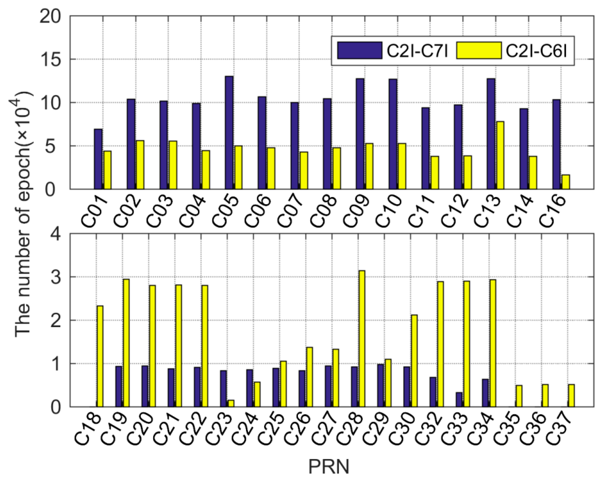
However, although more and more stations can track BDS-3 satellites, the number of the BDS-3 satellite is still less than that of the BDS-2 satellite. Figure 2 demonstrates the monthly mean of available epochs for BDS, which shows that the number of available epochs for BDS-2 is several times larger than that for BDS-3. The reason could be related to the fact that BDS-3 has not been completed completely. For BDS-2, the number of available epochs for C2I–C7I is more than that for C2I–C6I since more stations can track C2I and C7I observations of BDS-2. However, the number of available epochs for C16 is less than other satellites, which may be attributed to the late launch and operation of the C16 satellite. In terms of BDS-3, the number of available epochs for C2I–C6I is larger than that for C2I–C7I except for C23 and C24, which may be attributed to the more stations that can track C2I and C6I observations of BDS-3. Furthermore, the number of available observations for BDS-3 satellites is not as stable as that for BDS-2.
2.2. DCB Estimation Based on GIM
The slant TEC (STEC) can be obtained by the geometry-free observations when ignoring the higher order effects of the ionosphere, which can be written as follows [33]:
where and denote the pseudo range observations at the frequency and , respectively; refers to the slant total electron content in the signal propagation path between GNSS satellites and ground receivers; represents the speed of light in vacuum; and denote the receiver and satellite DCB, respectively. represents the vertical TEC along the vertical direction upon the ionospheric pierce points. represents the single layer mapping function for converting STEC to VTEC, which can be defined as follows [34]:
where refers to the average radius of the Earth; denotes the assumed single-layer ionosphere height; and denote the satellite zenith angles of a satellite at the receiver and the corresponding IPP, respectively.
As is well known, Equation (1) is used for the receiver and satellite DCB estimation. For the sake of convenience, ionospheric delays of Equation (1) is eliminated by using an existing GIM provided by Center for Orbit Determination in Europe (CODE) [16]. The DCBs of satellite and receiver are estimated as one constant per day, respectively, while a 20° cutoff elevation angle is set to mitigate multipath errors. Thus, the total values of satellite plus receiver DCB can be expressed as below:
where refers to the total number of epochs in the signal propagation path between the receiver and satellite ; k refers to the epoch. The correlation between satellite and receiver DCB leads to the singular system of normal equations. The zero-mean condition on satellite DCBs needs to be adopted, which can be defined as below [34]:
where denotes the total number of BDS satellites. Furthermore, we estimate the receiver and satellite DCB by adopting two solutions (BDS-2 + BDS-3, BDS-2-only) to analyze the impacts on satellite and receiver DCB after combing with BDS-3 observations. The estimated method also can be used for DCB estimation of other GNSS. However, the part of the analysis is mainly for BDS. The DCB of satellite and one particular receiver for the two solutions can be expressed as:
where refers to the total number of satellites available of BDS-2 and BDS-3 while denotes the total number of satellites available of BDS-2, with and representing the sum of satellite plus receiver DCB for two solutions, respectively.
It should be noted that the zero-mean condition is different under the two solutions due to the difference in the number of satellites between the two solutions. This difference brings about a bias of DCB for the same satellite and the receiver of the same station between the two solutions. Thus making it impossible to directly compare the BDS-2 satellite DCB and receiver DCB calculated by the two solutions. To implement the analysis of DCB estimated by the two solutions, it is necessary to unify the zero-mean conditions of BDS-2 + BDS-3 solutions to that of BDS-2 solutions. In other words, the zero-mean conditions of BDS-2 + BDS-3 solution need to be changed from to . Therefore, the values of satellite DCB and receiver DCB need to be corrected correspondingly due to the change of zero-mean condition [16]. The zero-mean condition of BDS-2 + BDS-3 solution can be expressed as:
As it can be seen, in order to satisfy the changed zero-mean condition, the satellite DCB of BDS-2 + BDS-3 solution need to be corrected with an increment of . Thus, the corrected satellite DCB of BDS-2 + BDS-3 solution can be expressed as:
For receiver DCB of a station, before and after the change of zero-mean condition, it can be expressed as:
where refers to the number of satellites the station can track; represents the sum of satellite DCB plus receiver DCB. From Equations (7) and (8), due to the constant value of , the DCB value of each satellite is corrected with an increment, and the corresponding receiver DCB also needs to be corrected. It can be expressed as:
Therefore, based on Equations (7)–(9), the zero mean conditions of the two solutions are unified, and comparison and analysis between the BDS-2 satellite DCB and receiver DCB estimated by the two solutions can be conducted.
3. Results and Discussion
3.1. Estimation of BDS-3 Satellite DCB
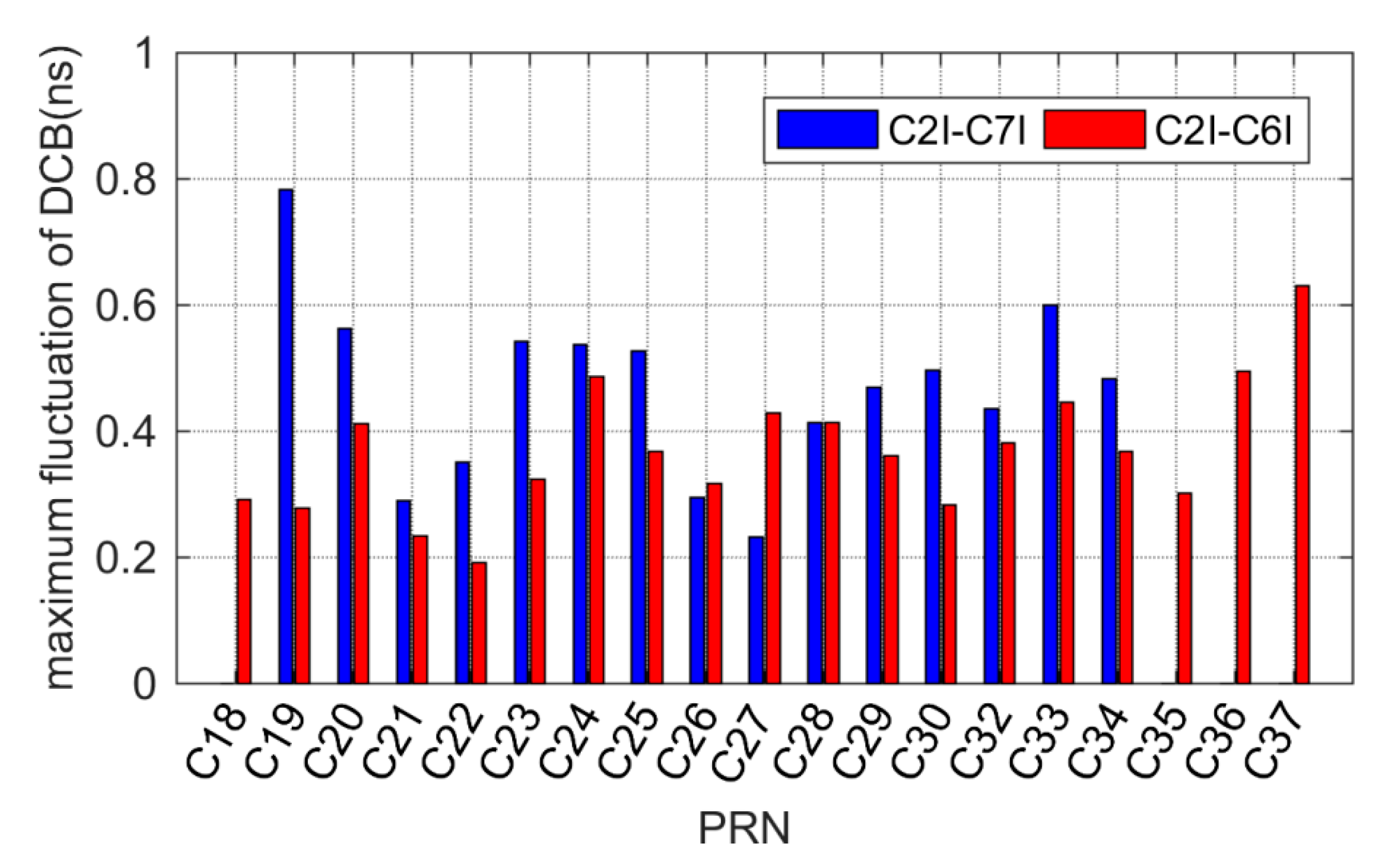
In our study, the BDS-3 DCBs are estimated based on the MGEX observations during the period of DOY 002–031, 2019. Figure 3 reprents the BDS-3 satellite C2I–C7I and C2I–C6I DCBs time series value, showing that the BDS-3 satellite DCB varies between -25 and 20 ns. A small periodic oscillation can be found in the time series of all satellites (except C18) DCB, because all satellites (except C18 as an inclined geosynchronous satellite orbit (IGSO) satellite) are medium Earth orbit (MEO) satellites and this variation may be related to the characteristic of one-week repeat ground track for MEO satellites. Furthermore, periodic ground track may exert a systematic impact on the tracking network, which will lead to the small period oscillation of the MEO satellite DCB [14]. On DOY 011–013 and DOY 016–017, 2019, all satellites show small jump since nothing was observed from C2I–C6I of C18 satellite. Furthermore, the monthly maximum fluctuation of BDS-3 satellite C2I–C7I and C2I–C6I DCB, presented in Figure 4, showing that the maximum fluctuations of mostly satellites are within 0.6 ns. The maximum fluctuations of C2I–C7I DCB for most satellites are larger than those of C2I–C6I because of the fewer C2I–C7I observations for BDS-3 satellites. As shown in the DCB time series value, our estimated BDS-3 satellites DCB are stable.
To further verify our estimated BDS-3 satellite DCB, the estimated DCB was evaluated with refernece to the BDS DCB products provided by CAS and DLR. The bias and standard deviation (STD) of our estimated BDS-3 satellite DCB with respect to the CAS and DLR are shown in Figure 5, while the products of BDS-3 C2I–C7I are not provided by DLR during the period of DOY 2–31, 2019. It can be seen that our estimated BDS-3 DCB shows good agreement with CAS and DLR. The bias of BDS-3 C2I–C7I and C2I–C6I DCB is less than 0.2 ns, with the STDs of mostly less than 0.2 ns. For C2I–C7I DCB, the mean bias and STD with respect to the CAS are 0.06 and 0.18 ns, respectively, while those for C2I–C6I DCB are 0.09 and 0.15 ns, and the values with respect to the DLR are 0.10 and 0.13 ns, respectively. Compared with the C2I–C7I DCB, the bias of C2I–C6I DCB with respect to CAS/DLR shows a larger value, because fewer C2I–C6I observations are available for some satellites (e.g., C23, C24, C35, C36, and C37). However, the STDs of C2I–C6I DCB with respect to CAS/DLR are less than those of C2I–C7I DCB, which may probably be related to ionk of Equation (3) [16]. According to the Equation (3), , we can know that the impact on the DCB caused by ionospheric errors is related to ionk. C2I–C6I DCB is less affected by ionospheric errors than C2I–C7I DCB due to the ionk of C2I–C6I is smaller than that of C2I–C7I. Thus, the STD of C2I–C6I DCB is smaller than that of C2I–C7I DCB, indicating that C2I–C6I DCB is more stable than C2I–C7I.
Furthermore, due to the differences of different GIMs, it is necessary to compare the DCB estimated using different GIMs. However, the GIM is not provided by DLR. Therefore, we estimate the BDS-3 DCB using the GIM from CAS for 30 days (DOY 2–31, 2019) as test cases. The mean differences and STD between estimated BDS-3 DCB using GIM from CODE and CAS are shown in Figure 6. It can be seen that the mean difference and STD are mostly less than 0.1 ns. In fact, the difference between the GIM provided by CODE and CAS has a very small impact on DCB estimation.
3.2. Analysis of Satellite DCB
In order to analyze the differences of satellite DCB before and after adding BDS-3 observations, we estimate the BDS-2 satellite DCB by adopting BDS-2 + BDS-3 and BDS-2-only solutions. Figure 7 shows the differences in BDS-2 satellite DCB between two solutions. For C2I–C7I DCB, the mean value of differences are within ±0.05 ns, with the relatively stable difference during this period. However, the differences present larger mean values in C2I–C6I DCB, especially in the C16 satellite, for which, their fewer observations may be responsible, with their mean values mostly within ±0.1 ns. Compared with the two types of DCB, the differences of C2I–C6I DCB show obvious fluctuations because the fewer C2I–C6I observations of BDS-2 are available. It can be seen that the fluctuation of differences for the IGSO satellite (except for C16) is lower than that for MEO and geostationary earth orbit (GEO) satellites. In addition, a small oscillation can be found in the MEO satellite (e.g., C11, C12, and C14), which is related to the characteristic of a one-week repeat ground track for the MEO satellite [14]. In short, it is indicated that the values of effect on BDS-2 satellite DCB after combing with BDS-3 observations are close to 0. Therefore, it can be concluded that there is no evident systematic bias between the processed DCB by before and after combing with BDS-3 observations.
Figure 8 shows the STD of our estimated BDS-2 satellite DCB and the products of CAS/DLR, clearly showing that the two solutions and DLR show the same scales of STD. The mean STD of C2I–C7I DCB for BDS-2 + BDS-3 solution, BDS-2-only solution, CAS and DLR is 0.10, 0.10, 0.31, and 0.11 ns, respectively, with the mean STD of C2I–C6I DCB for them as 0.09, 0.09, 0.15, and 0.12 ns, respectively. The mean STD of DCB for different BDS satellites is given in Table 1. The results of the two solutions in Table 1 are almost identical, indicating that the STDs of BDS-2 satellite DCB for both BDS-2 + BDS-3 and BDS-2-only solutions are at the same level. In other words, there is no significant change in the stability of BDS-2 satellite DCB when combing with BDS-3 observations.
3.3. Analysis of Receiver DCB
Similarly, to analyze the impacts on the receiver DCB after combining with BDS-3 observations, we estimate the BDS receiver DCB by adding BDS-2 + BDS-3 and BDS-2-only solutions. Since fewer C2I–C7I observations can be tracked by BDS-3, the C2I–C6I receiver DCBs are mainly analyzed in this section. Table 2 lists the detailed information of these stations that can track both BDS-3 and BDS-2 simultaneously.
Figure 9 shows the mean differences and STDs of receiver C2I–C6I DCB between BDS-2 + BDS-3, and BDS-2-only solutions. It obviously shows that the mean differences and STDs are mostly within ±1.5 and 0.3 ns, respectively, with their mean values as 0.04 and 0.14 ns, respectively. It indicates that the mean differences of receiver C2I–C6I DCB between the two solutions are close to 0. Furthermore, it can be found that the characteristics of the difference are related to receiver type. For these stations with the same receiver type (e.g., JAVAD, SEPT POL, and TRIMBLE), the differences of receiver C2I–C6I DCB between the two solutions are similar. In terms of these stations whose receiver type is JAVAD, SEPT POL, and TRIMBLE, corresponding to stations index 1–24, 25–66 and 67–106, the differences are all positive, negative, and around 0. However, the two stations (BRST and GANP) with TRIMBLE receiver reveal larger difference, because they just track can fewer observations. It can thus be concluded that the effect exerted by BDS-3 observations on receiver DCB is related to the receiver type. The effect for those stations whose receiver type is TRIMBLE is the lowest, followed by SEPT POL and JAVAD.
Moreover, the STD of receiver C2I–C6I DCB for the two solutions is shown in Figure 10, with the stations being aligned by geomagnetic latitudes at the horizontal axis. It can be seen that the STDs of receiver DCB for the two solutions are mostly less than 0.4 ns, with the larger values of STD being more likely to exist at low latitudes. It indicates that receiver DCBs have a latitudinal dependence. This phenomenon has also been reported for other in some previous studies on receiver DCB for other GNSS [35]. Compared with the STD of the two solutions, the values of BDS-2 + BDS-3 solution are smaller than those of BDS-2-only solution for most stations, with their mean values being 0.24, and 0.28 ns, respectively. It can be concluded that this stability of receiver DCB is better when BDS-3 observations are added.
4. Conclusions
In this paper, the BDS DCBs are estimated and analyzed by using the MGEX observations during the period of DOY 2–31, 2019. Our estimated BDS-3 DCB shows good agreement with CAS and DLR. The bias of BDS-3 C2I–C7I and C2I–C6I DCB are within ±0.2 ns, and the STDs are mostly within 0.2 ns. For C2I–C7I DCB, the mean bias and STDs with respect to the CAS are 0.06 and 0.18 ns, respectively. For C2I–C6I DCB, the mean bias and STDs with respect to the CAS are 0.09 and 0.15 ns, and the values with respect to the DLR are 0.10 and 0.13 ns, respectively. In order to analyze the effects on both satellite and receiver DCB after combining BDS-3 observations, BDS-2 + BDS-3 and BDS-2-only solutions are used to estimate the satellite and receiver DCBs. For BDS-2 satellite DCB, the values of effect are close to 0, with the very limited effect on stability of DCB. For receiver DCB, 106 stations with C2I–C6I observations are collected to conduct analysis. The value of effect on each station is related to the receiver type, but their mean value is close to 0, and the stability of the receiver DCB is better when BDS-3 observations are added. Therefore, it can be concluded that there is no evident systematic bias between BDS-2 and BDS-2 + BDS-3 DCB.
Author Contributions
Conceptualization of the Manuscript Idea: Q.W. and S.J.; Methodology and Software: Q.W., J.C., and J.G.; Writing-Original Draft Preparation: Q.W. and L.Y.; Writing-Review and Editing: S.J. and Y.H.; Supervision and Funding Acquisition: S.J. All authors have read and agreed to the published version of the manuscript.
Funding
This work was supported by the National Natural Science Foundation of China-German Science Foundation (NSFC-DFG) Project (Grant No. 41761134092), Startup Foundation for Introducing Talent of NUIST (Grant No. 2243141801036) and Jiangsu Province Distinguished Professor Project (Grant No. R2018T20).
Acknowledgments
The authors gratefully acknowledged the DLR and CAS for providing products and IGS for providing MGEX data. The first author would like to acknowledge his wife and parents for their support and encouragement.
Conflicts of Interest
The authors declare no conflict of interest.
References
- Su, K.; Jin, S.G. Triple-frequency carrier phase precise time and frequency transfer models for BDS-3. GPS Solut. 2019, 23, 86. [Google Scholar] [CrossRef]
- CSNO. BeiDou navigation satellite system signal in space interface control document. In Open Service Signal B1I (Version 3.0); China Satellite Navigation Office: Beijing, China, 2019. [Google Scholar]
- Yang, Y.; Li, J.; Xu, J.; Tang, J.; Guo, H.; He, H. Contribution of the Compass satellite navigation system to global PNT users. Chin. Sci. Bull. 2011, 56, 2813–2819. [Google Scholar] [CrossRef] [Green Version]
- Kao, S.-P.; Chen, Y.-C.; Ning, F.-S. A MARS-based method for estimating regional 2-D ionospheric VTEC and receiver differential code bias. Adv. Space Res. 2014, 53, 190–200. [Google Scholar] [CrossRef]
- Abdelazeem, M.; Çelik, R.N.; El-Rabbany, A. MGR-DCB: A precise model for multi-constellation GNSS receiver differential code bias. J. Navig. 2016, 69, 698–708. [Google Scholar] [CrossRef] [Green Version]
- Sanz, J.; Juan, J.M.; Rovira-Garcia, A.; González-Casado, G. GPS differential code biases determination: Methodology and analysis. GPS Solut. 2017, 21, 1549–1561. [Google Scholar] [CrossRef] [Green Version]
- Lanyi, G.E.; Roth, T. A comparison of mapped and measured total ionospheric electron content using global positioning system and beacon satellite observations. Radio Sci. 1988, 23, 483–492. [Google Scholar] [CrossRef]
- Choi, B.K.; Sang, J.L. The Influence of Grounding on GPS Receiver Differential Code Biases. Adv. Space Res. 2018, 62, 457–463. [Google Scholar] [CrossRef]
- Themens, D.R.; Jayachandran, P.; Langley, R.B. The nature of GPS differential receiver bias variability: An examination in the polar cap region. J. Geophys. Res. Space Phys. 2015, 120, 8155–8175. [Google Scholar] [CrossRef]
- Mylnikova, A.; Yasyukevich, Y.V.; Kunitsyn, V.; Padokhin, A. Variability of GPS/GLONASS differential code biases. Results Phys. 2015, 5, 9–10. [Google Scholar] [CrossRef] [Green Version]
- Ma, G.; Gao, W.; Li, J.; Chen, Y.; Shen, H. Estimation of GPS instrumental biases from small scale network. Adv. Space Res. 2014, 54, 871–882. [Google Scholar] [CrossRef]
- Xue, J.; Song, S.; Zhu, W. Estimation of differential code biases for Beidou navigation system using multi-GNSS observations: How stable are the differential satellite and receiver code biases? J. Geod. 2015, 90, 309–321. [Google Scholar] [CrossRef]
- Wei, C.; Zhang, Q.; Fan, L.; Zhang, S.; Huang, G.; Chen, K. Estimate DCB of BDS satellites based on the observations of GPS/BDS. In Proceedings of the China Satellite Navigation Conference (CSNC) 2014 Proceedings, Nanjing, China, 21–23 May 2014; Volume 2, pp. 351–362. [Google Scholar]
- Wang, N.; Yuan, Y.; Li, Z.; Montenbruck, O.; Tan, B. Determination of differential code biases with multi-GNSS observations. J. Geod. 2015, 90, 209–228. [Google Scholar] [CrossRef]
- Shi, C.; Fan, L.; Li, M.; Liu, Z.; Gu, S.; Zhong, S.; Song, W. An enhanced algorithm to estimate BDS satellite’s differential code biases. J. Geod. 2015, 90, 161–177. [Google Scholar] [CrossRef]
- Jin, S.; Jin, R.; Li, D. Assessment of BeiDou differential code bias variations from multi-GNSS network observations. Ann. Geophys. 2016, 34, 259–269. [Google Scholar] [CrossRef] [Green Version]
- Fan, L.; Li, M.; Wang, C.; Shi, C. BeiDou satellite’s differential code biases estimation based on uncombined precise point positioning with triple-frequency observable. Adv. Space Res. 2017, 59, 804–814. [Google Scholar] [CrossRef]
- Zhang, R.; Song, W.W.; Yao, Y.B.; Shi, C.; Lou, Y.D.; Yi, W.T. Modeling regional ionospheric delay with ground-based BeiDou and GPS observations in China. GPS Solut. 2015, 19, 649–658. [Google Scholar] [CrossRef]
- Ren, X.; Zhang, X.; Xie, W.; Zhang, K.; Yuan, Y.; Li, X. Global ionospheric modelling using multi-GNSS: BeiDou, Galileo, GLONASS and GPS. Sci. Rep. UK 2016, 6, 33499. [Google Scholar] [CrossRef] [Green Version]
- Abdelazeem, M.; Çelik, R.N.; El-Rabbany, A. An accurate Kriging-based regional ionospheric model using combined GPS/BeiDou observations. J. Appl. Geod. 2018, 12, 65–76. [Google Scholar] [CrossRef]
- Jin, S.; Jin, R.; Kutoglu, H. Positive and negative ionospheric responses to the March 2015 geomagnetic storm from BDS observations. J. Geod. 2017, 91, 613–626. [Google Scholar] [CrossRef]
- Li, Z.; Yuan, Y.; Fan, L.; Huo, X.; Hsu, H. Determination of the Differential Code Bias for Current BDS Satellites. IEEE Trans. Geosci. Remote Sens. 2014, 52, 3968–3979. [Google Scholar] [CrossRef]
- Jin, R.; Jin, S.; Feng, G. M_DCB: Matlab code for estimating GNSS satellite and receiver differential code biases. GPS Solut. 2012, 16, 541–548. [Google Scholar] [CrossRef]
- Zhang, Q.; Zhao, Q. Global Ionosphere Mapping and Differential Code Bias Estimation during Low and High Solar Activity Periods with GIMAS Software. Remote Sens. 2018, 10, 705. [Google Scholar] [CrossRef] [Green Version]
- Montenbruck, O.; Hauschild, A.; Steigenberger, P. Differential Code Bias Estimation using Multi-GNSS Observations and Global Ionosphere Maps. Navigation 2014, 61, 191–201. [Google Scholar] [CrossRef]
- Li, X.; Xie, W.; Huang, J.; Ma, T.; Zhang, X.; Yuan, Y. Estimation and analysis of differential code biases for BDS3/BDS2 using iGMAS and MGEX observations. J. Geod. 2019, 93, 419–435. [Google Scholar] [CrossRef]
- Li, X.; Ma, T.; Xie, W.; Zhang, K.; Huang, J.; Ren, X. FY-3D and FY-3C onboard observations for differential code biases estimation. GPS Solut. 2019, 23, 57. [Google Scholar] [CrossRef]
- Li, Z.; Yuan, Y.; Li, H.; Ou, J.; Huo, X. Two-step method for the determination of the differential code biases of COMPASS satellites. J. Geod. 2012, 86, 1059–1076. [Google Scholar] [CrossRef]
- Zhang, B.; Ou, J.; Yuan, Y.; Li, Z. Extraction of line-of-sight ionospheric observables from GPS data using precise point positioning. Sci. China Earth Sci. 2012, 55, 1919–1928. [Google Scholar] [CrossRef]
- Rizos, C.; Montenbruck, O.; Weber, R.; Weber, G.; Neilan, R.; Hugentobler, U. The IGS MGEX experiment as a milestone for a comprehensive multi-GNSS service. In Proceedings of the Institute of Navigation Pacific Positioning, Navigation and Timing (ION Pacific PNT), Honolulu, HI, USA, 23–25 April 2013; pp. 289–295. [Google Scholar]
- Montenbruck, O.; Steigenberger, P.; Prange, L.; Deng, Z.; Zhao, Q.; Perosanz, F.; Romero, I.; Noll, C.; Stürze, A.; Weber, G. The Multi-GNSS Experiment (MGEX) of the International GNSS Service (IGS)–achievements, prospects and challenges. Adv. Space Res. 2017, 59, 1671–1697. [Google Scholar] [CrossRef]
- Montenbruck, O.; Steigenberger, P.; Khachikyan, R.; Weber, G.; Langley, R.; Mervart, L.; Hugentobler, U. IGS-MGEX: Preparing the ground for multi-constellation GNSS science. Inside Gnss 2014, 9, 42–49. [Google Scholar]
- Wellenhof, B.H.; Lichtenegger, H.; Collins, J. Global Positioning System: Theory and Practice; Science & Business Media: Berlin, Germany, 1992. [Google Scholar]
- Schaer, S. Mapping and Predicting the Earth’s Ionosphere Using the Global Positioning System; Astronomical Institute, University of Berne: Bern, Switzerland, 1999. [Google Scholar]
- Li, M.; Yuan, Y.; Wang, N.; Li, Z.; Li, Y.; Huo, X. Estimation and analysis of Galileo differential code biases. J. Geod. 2016, 91, 279–293. [Google Scholar] [CrossRef]
Figure 1.
Distribution of Multi-Global Navigation Satellite System (GNSS) Experiment (MGEX) tracking stations with BeiDou Navigation Satellite System (BDS). The red color represents the stations that only support tracking of BDS-2 satellites, green color represents the stations that support tracking of BDS-2 and BDS-3 satellites simultaneously.

Figure 2.
Mean values of available epochs for BDS-2 (top plot) and BDS-3 (bottom plot).

Figure 3.
Time series of BDS-3 satellite C2I–C7I and C2I–C6I DCBs.

Figure 4.
Monthly maximum fluctuation of BDS-3 satellite DCB.

Figure 5.
Bias and Standard Deviation (STD) of BDS-3 C2I–C7I (top plot) and C2I–C6I (bottom plot) DCB with respect to Chinese Academy of Sciences (CAS)/Deutsche Zentrum für Luft- und Raumfahrt (DLR).
Figure 5.
Bias and Standard Deviation (STD) of BDS-3 C2I–C7I (top plot) and C2I–C6I (bottom plot) DCB with respect to Chinese Academy of Sciences (CAS)/Deutsche Zentrum für Luft- und Raumfahrt (DLR).

Figure 6.
Mean differences and STD between estimated BDS-3 C2I–C7I (top plot) and C2I–C6I (bottom plot) DCB using global ionospheric map (GIM) from the CODE and CAS
Figure 6.
Mean differences and STD between estimated BDS-3 C2I–C7I (top plot) and C2I–C6I (bottom plot) DCB using global ionospheric map (GIM) from the CODE and CAS

Figure 7.
Difference in BDS-2 satellite DCB between BDS-2 + BDS-3 and BDS-2-only solutions. M1 and M2 represent mean differences of C2I–C7I and C2I–C6I DCB, respectively.
Figure 7.
Difference in BDS-2 satellite DCB between BDS-2 + BDS-3 and BDS-2-only solutions. M1 and M2 represent mean differences of C2I–C7I and C2I–C6I DCB, respectively.

Figure 8.
STDs of BDS-2 satellite C2I–C7I (top plot) and C2I–C6I (bottom plot) DCB.

Figure 9.
Mean differences and STDs of receiver C2I–C6I DCB between BDS-2 + BDS-3 and BDS-2-only solutions.
Figure 9.
Mean differences and STDs of receiver C2I–C6I DCB between BDS-2 + BDS-3 and BDS-2-only solutions.

Figure 10.
Scatters of STD of receiver C2I–C6I DCBs versus geomagnetic latitudes.


Table 1.
STD of BDS-2 satellite DCB for two solutions (units: ns).
| Type | [BDS-2 + BDS-3] | [BDS-2-Only] | ||||||
|---|---|---|---|---|---|---|---|---|
| GEO | IGSO | MEO | Mean | GEO | IGSO | MEO | Mean | |
| C2I–C7I | 0.14 | 0.05 | 0.10 | 0.10 | 0.14 | 0.05 | 0.10 | 0.10 |
| C2I–C6I | 0.12 | 0.06 | 0.09 | 0.09 | 0.11 | 0.05 | 0.10 | 0.09 |
Table 2.
Receiver and stations involved in the estimation of BDS-3 C2I–C6I DCBs.
| Receiver Type | Stations Index | Stations Name |
|---|---|---|
| JAVAD TRE_3 | 1–5 | POTS, SGOC, ULAB, URUM, WUH2 |
| JAVAD TRE_3 DELTA | 6–23 | CRO1, GCGO, GODN, GODS, MGO3, QUIN, LPGS, CUSV, ARHT, BOGT, BSHM, MBAR, MET3, MOIU, POL2, SOD3, STHL, ZAMB |
| JAVAD TRE_G3TH DELTA | 24 | FFMJ |
| SEPT POLARX5 | 25–53 | MRC1, ABPO, VACS, AREG, ARUC, CEDU, CHPI, DARW, DAV1, DGAR, FALK, GOP6, GRAZ, HOB2, IISC, JOZE, JPLM, KAT1, LAUT, MAW1, NRMG, PADO, POHN, PTGG, SUTH, TID1, TONG, YAR3, YARR |
| SEPT POLARX5TR | 54–66 | GODE, AMC4, USN7, BREW, GAMG, HARB, HERS, KOUG, MATZ, ROAG, STJ3, TLSG, YEL2 |
| TRIMBLE ALLOY | 67–68 | BRST, GANP |
| TRIMBLE NETR9 | 69–106 | CUT0, ASCG, CHPG, CPVG, DYNG, FTNA, GAMB, JFNG, KERG, MAYG, METG, NKLG, OWMG, RGDG, SEYG, TLSE, BELE, BOAV, BOR1, KIR8, KZN2, MCHL, MRO1, PERT, POAL, POVE, RDSD, SALU, SAVO, SIN1, TOPL, TUVA, UCAL, UFPR, UNB3, XMIS, ZIM2, ZIM3 |
© 2019 by the authors. Licensee MDPI, Basel, Switzerland. This article is an open access article distributed under the terms and conditions of the Creative Commons Attribution (CC BY) license (http://creativecommons.org/licenses/by/4.0/).
Share and Cite
MDPI and ACS Style
Wang, Q.; Jin, S.; Yuan, L.; Hu, Y.; Chen, J.; Guo, J. Estimation and Analysis of BDS-3 Differential Code Biases from MGEX Observations. Remote Sens. 2020, 12, 68. https://doi.org/10.3390/rs12010068
AMA Style
Wang Q, Jin S, Yuan L, Hu Y, Chen J, Guo J. Estimation and Analysis of BDS-3 Differential Code Biases from MGEX Observations. Remote Sensing. 2020; 12(1):68. https://doi.org/10.3390/rs12010068
Chicago/Turabian StyleWang, Qisheng, Shuanggen Jin, Liangliang Yuan, Youjian Hu, Jie Chen, and Jiabin Guo. 2020. "Estimation and Analysis of BDS-3 Differential Code Biases from MGEX Observations" Remote Sensing 12, no. 1: 68. https://doi.org/10.3390/rs12010068
Note that from the first issue of 2016, this journal uses article numbers instead of page numbers. See further details here.