Multisource Point Clouds, Point Simplification and Surface Reconstruction
by
 , , ,
, , ,
Lingli Zhu
1,*, 
Antero Kukko
1,
Juho-Pekka Virtanen
2,
Juha Hyyppä
1,
Harri Kaartinen
1,3,
Hannu Hyyppä
3 and
Tuomas Turppa
1 1
Department of Remote Sensing and Photogrammetry, Finnish Geospatial Research Institute, 02430 Masala, Finland
2
Department of Built Environment, School of Engineering, Aalto University, 02150 Espoo, Finland
3
Department of Geography and Geology, University of Turku, 20014 Turun, Finland
*
Author to whom correspondence should be addressed.
Remote Sens. 2019, 11(22), 2659; https://doi.org/10.3390/rs11222659
Submission received: 15 October 2019
/
Revised: 11 November 2019
/
Accepted: 12 November 2019
/
Published: 13 November 2019
(This article belongs to the Section Engineering Remote Sensing)
Abstract
:As data acquisition technology continues to advance, the improvement and upgrade of the algorithms for surface reconstruction are required. In this paper, we utilized multiple terrestrial Light Detection And Ranging (Lidar) systems to acquire point clouds with different levels of complexity, namely dynamic and rigid targets for surface reconstruction. We propose a robust and effective method to obtain simplified and uniform resample points for surface reconstruction. The method was evaluated. A point reduction of up to 99.371% with a standard deviation of 0.2 cm was achieved. In addition, well-known surface reconstruction methods, i.e., Alpha shapes, Screened Poisson reconstruction (SPR), the Crust, and Algebraic point set surfaces (APSS Marching Cubes), were utilized for object reconstruction. We evaluated the benefits in exploiting simplified and uniform points, as well as different density points, for surface reconstruction. These reconstruction methods and their capacities in handling data imperfections were analyzed and discussed. The findings are that (i) the capacity of surface reconstruction in dealing with diverse objects needs to be improved; (ii) when the number of points reaches the level of millions (e.g., approximately five million points in our data), point simplification is necessary, as otherwise, the reconstruction methods might fail; (iii) for some reconstruction methods, the number of input points is proportional to the number of output meshes; but a few methods are in the opposite; (iv) all reconstruction methods are beneficial from the reduction of running time; and (v) a balance between the geometric details and the level of smoothing is needed. Some methods produce detailed and accurate geometry, but their capacity to deal with data imperfection is poor, while some other methods exhibit the opposite characteristics.
1. Introduction
As the diversity, ease of use and popularity of three dimensional (3D) acquisition methods continue to increase, so does the need for the development of new techniques for surface reconstruction [1]. The focus of surface reconstruction has shifted in recent years from the early stage of piecewise linear reconstruction to handling the data imperfections caused by, e.g., occlusion and reflective materials. Some well-known algorithms, such as Alpha shapes [2], Ball pivoting [3], Poisson reconstruction, the Crust [4,5] and Algebraic point set surfaces (APSS or APSS Marching Cubes) [6], have proven their effectiveness for certain object reconstruction scenarios. However, multi-sourced data from various scenes with data imperfection are challenging the methods of surface reconstruction. It is necessary to know how these classic algorithms handle the challenge of datasets from state-of-the-art light detection and ranging (Lidar) technologies, and to indicate the direction of future development.
Multi-sourced data has been acquired by terrestrial Lidar with different platforms: static tripod, movable trolley and handheld style. These systems have different advantages and disadvantages. Thus, different types of objects can be collected. A static terrestrial Lidar is operated in one station along or around the target (e.g., an object or a scene). Multiple featured objects (e.g., typically using white, spherical objects) are placed in the scene so that the data measured from neighboring stations can be matched by these features. A car has been scanned by such a static Lidar system. While acquiring the data of a human body, it is challenging to stay still for that time period. Therefore, it is necessary to have multiple static Lidar systems operating from different directions at the same time to shorten the time of measurement. Although the static terrestrial Lidar is capable of highly accurate measurement, it has low efficiency. Additionally, it may encounter more occlusions due to the inflexibility of the platform. In contrast, a mobile platform is more flexible and highly efficient. In an indoor environment, a mobile Lidar system is one or more Lidar sets mounted on a mobile platform, e.g., a trolley or personal backpack, or in a hand-held style. Among these platforms, the hand-held system produces the least occluded data due to its flexibility and small volume. Thus, it can avoid occlusions to the greatest extent. Point clouds acquired by a Lidar system often have noise and holes due to, e.g., reflective materials (e.g., metal or glass), from the scene, occlusions, reflections from sunlight, errors from measurement, and so on. Different surface reconstruction methods handle data imperfection differently.
Apart from data imperfection, a huge amount of point clouds has been produced from Lidar systems. State-of-the-art laser scanning technology can produce several million points per second. Such a huge amount of data, on the one hand, provide data with high accuracy; on the other hand, it is a challenge to perform follow-up processing, e.g., 3D surface reconstruction and rendering. To reduce the workload during the reconstruction, point simplification has become considerably important. In previous studies, feature-based methods were mostly introduced by, e.g., Cohen et al., 2004 [7]; Song & Feng, 2009 [8]; Leal et al., 2017 [9]; Chen et al., 2017 [10]; Qi et al., 2018 [11]. The most common problems with these methods were that a) the resultant point cloud was not uniform; and b) it was a challenge to maintain a balance between loss in features and loss in accuracy. In this paper, we will address a reliable, robust and effective solution for the above problems.
The objectives of the paper are to propose an approach to simplify the point cloud and obtain uniform resampled points with minimized accuracy loss, to study how the uniformity of points affects the surface reconstruction, to figure out how the number of points and the density of points affect the surface reconstruction and to analyze the differences of different surface reconstruction algorithms in handling data imperfection.
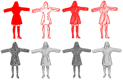
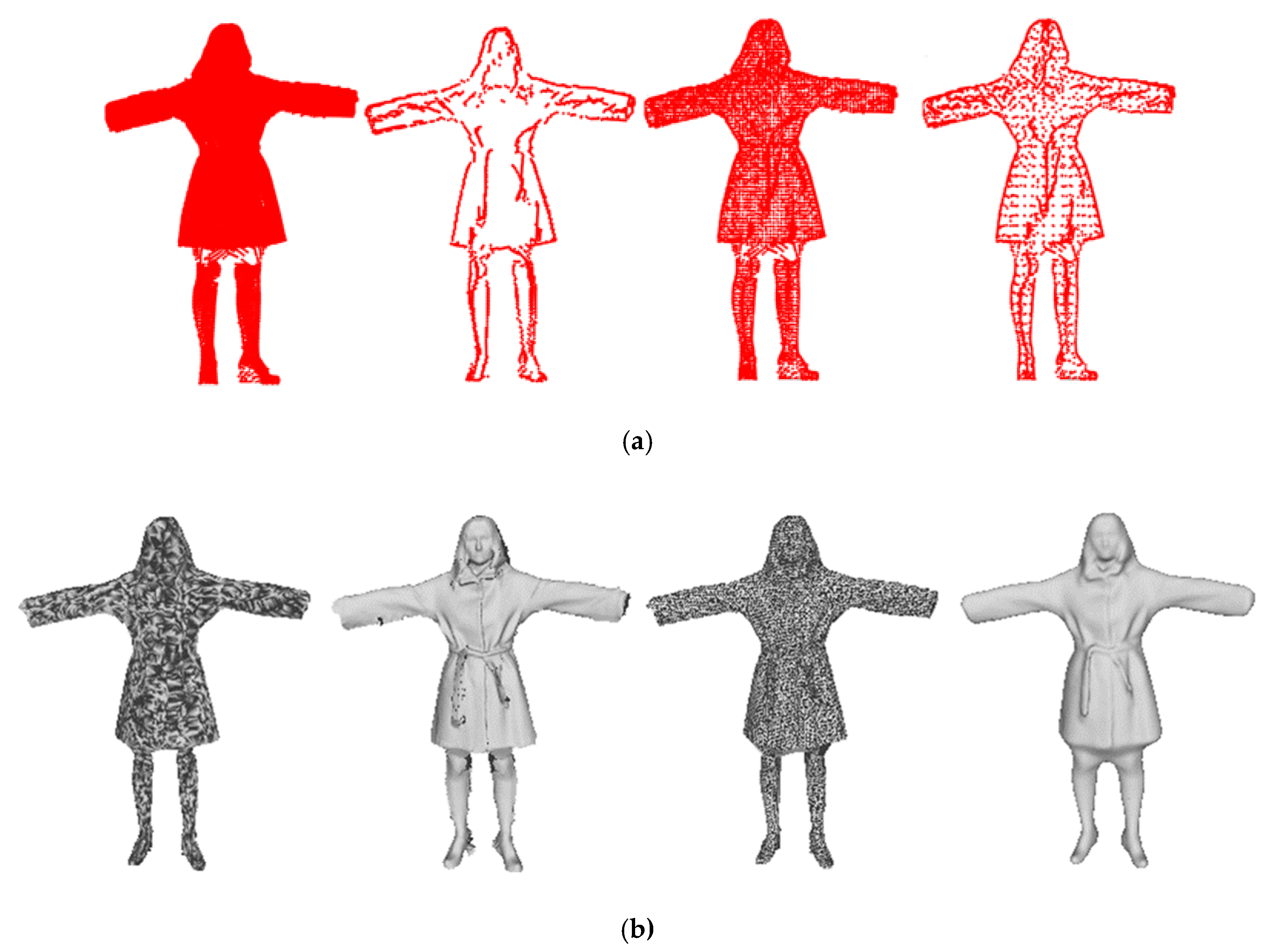
The idea of our point cloud simplification method is to separate the key characteristics of an object from the least important points by using Principal Component Analysis (PCA) and multi-view projection geometry and to resample these points using different grid sizes (e.g., key characteristics use a small grid size, while the least important points use a big grid size) to minimize the loss of accuracy. Then, the resampled key points (also called edge points in this paper) are merged with the resampled remaining points. Surfaces are reconstructed by exploiting four well-known methods: Alpha shapes, power crust, APSS, and Screened Poisson Reconstruction (SPR). The results are compared and analyzed, and their advantages and disadvantages, and the direction of future development, are addressed. Figure 1 illustrates an overview of the procedure of point cloud simplification and the use of different methods for surface reconstruction.
2. Related Works
Studies related to point cloud simplification and object surface reconstruction have been highlighted for decades. Over time, as the hardware continuously advanced, methods are constantly improved and upgraded. In this paper, related work is focused on two aspects: point cloud simplification and surface reconstruction.
2.1. Point Cloud Simplification and Uniformity
Among point cloud simplification methods, feature-based methods and random sampling methods have been highlighted. Cohen-Steiner et al. (2004) [7] introduced a variational shape approximation approach by utilizing error-driven optimizations of a partition and a set of local proxies to provide geometric representations. However, the efficiency was low. Leal et al. (2017) [9] presented a point cloud simplification method by estimating the local density to cluster the point cloud, identifying the points with a high curvature to remain, and applying a linear programming model to reduce the point cloud. Song and Feng (2009) [8] identified sharp edge points from the scanned mechanical part. Then, based on points in its neighborhood and corresponding to the point’s contribution to the representation of local surface geometry, the least important data point was removed. Chen et al. (2017) [10] introduced a resampling method that is guaranteed to be shift-, rotation- and scale-invariant in three-dimensional space. The resampling method utilizes a graph filtering based on all-pass, low-pass and high-pass graph filtering and graph filter banks. The resulting points on surfaces with indistinct features are all neglected. The above methods preserve distinct edge information and remove the least important data. This leads to the extreme non-uniformity of point density. However, uniformity is important in mesh-related applications. Qi et al. (2018) [11] addressed a point cloud simplification method that aims to strike a balance between preserving sharp features and maintaining uniform density during resampling by leveraging graph signal processing. The authors formulated the loss in features and the loss in uniformity during the process of simplification. Then, an optimal resampling matrix is found by minimizing the total loss. However, it is a challenge to strike such a balance.
With regard to the random sampling methods, the most well-known methods include Monte Carlo sampling [12] and Poisson disk sampling. Monte Carlo sampling uses a probability distribution function to generate uniformly distributed random numbers on a unit interval. Poisson disk sampling uses a disk that is centered in each sample. The minimum distance between samples is the diameter of the disk. Thus, uniform sampled points are produced.
Corsini et al. (2012) [13] proposed a constrained Poisson disk sampling method, which is currently adopted by Meshlab (www.meshlab.net) for point simplification. The constrained Poisson disk sampling method utilizes the geometric constraints on sample placement, and the authors suggested that biased Monte Carlo distributions should be avoided. This method makes the Poisson disk sampling method more flexible and effective.
2.2. Surface Reconstruction from Point Clouds
The approaches for surface reconstruction from point clouds are typically grouped into two categories: parametric surface reconstruction methods and triangulated surface reconstruction methods.
2.2.1. Parametric Surface Reconstruction Methods
These methods typically exploit parameters to adjust a set of initial models to fit the geometry of an object. The advantages lie in their flexibility, high efficiency and reuse capability. However, it is challenging to reconstruct complicated geometries. Studies concerning parametric surface reconstruction methods can be found in, e.g., Floater, 1997 [14]; Floater & Reimers, 2001 [15]; Gal et al., 2007 [16]; Lafarge & Alliez, 2013 [17]. The aforementioned Floater and Reimers (2001) [15] proposed a method to map the points into some convex parameter domain and obtain a corresponding triangulation of the original dataset by triangulating the parameter points. Gal et al. (2007) [16] proposed a surface reconstruction method by using a database of local shape priors. The method extracts similar parts from previously scanned models to create a database of examples, and forms a basis to learn typical shapes and details by creating local shape priors in the form of enriched patches. The patches serve as a type of training set for the reconstruction process. Lafarge and Alliez (2013) [17] proposed a structure-preserving approach to reconstruct the surfaces from both the consolidated components and the unstructured points. The authors addressed the common dichotomy between smooth/piecewise-smooth and primitive-based representations. The canonical parts from detected primitives and free-form parts of the inferred shape were combined. The final surface was obtained by solving a graph-cut problem formulated on the 3D Delaunay triangulation of the structured point set where the tetrahedra are labeled as inside or outside cells.
2.2.2. Triangulation/Mesh-based Algorithms
The most classic triangulation methods include Marching Cube reconstruction [18,19], Alpha Shapes reconstruction [2], the Ball-Pivoting surface reconstruction [3], the Power Crust [4], Cocone [20,21,22], Poisson surface reconstruction [23], Screened Poisson surface reconstruction [24], and Wavelet surface reconstruction [25]. The Marching cubes reconstruction method was first proposed by [18]. The authors used a divide-and-conquer approach to generate cube slices (voxels). Triangle vertices were calculated by using linear interpolation. A table of edge intersections was established to describe cube connectivity. The gradient information at a cube vertex was estimated by using central differences along the three coordinate axes, and the normal of each triangle vertex was interpolated. The resulting triangle vertices and vertex normal were the output. Later, the Marching cubes were evolved into the Marching tetrahedral [26] and Cubical Marching Squares [27]. A review of the Marching cubes methods can be found in [19,28].
In 1994, Edelsbrunner and Mucke (1994) [2] developed the concept of a 3D alpha shape from an intuitive description to a formal definition, implemented the algorithm and made the software available to the public. The idea of the 3D alpha shape was to draw the edges of an alpha shape by connecting neighboring boundary points and envelop all points within the dataset. The parameter α, as the alpha radius, controls the desired level of detail and determines different transitions in the shape. The typical drawback of such a method was low efficiency in computing the Delaunay triangulation of the points. Later, in 1997, Bernardini and Bajaj [29] further developed the alpha shapes algorithm for reconstruction.
The authors proposed that a regularization could eliminate dangling and isolated faces, edges and points from the alpha shapes, and they improved the resulting approximate reconstruction in areas of insufficient sampling density. After two years, Bernardini et al. (1999) [3] introduced the ball-pivoting algorithm (BPA) for surface reconstruction. It retains some of the qualities of alpha shapes. The idea of the Ball-Pivoting algorithm is to pivot a ball with specific radius R over the points and touch three points, without containing any other point, to form a triangle. Then the ball starts from an edge of the seed triangle and touches another point to form the next triangle. The process is repeated until all points are allocated in triangles. This method improved efficiency.
The power crust algorithm was first proposed by Amenta et al. [4]. The idea was to construct piecewise-linear approximations to both the object surface and medial axis transform (MAT). It is a Voronoi diagram-based method. The Voronoi diagram was applied to approximate the MAT from the input points, and the power diagram was used to produce a piecewise-linear surface approximation from the MAT, which was an inverse transform. This method was effective at resisting noise and eliminating holes in the original data.
The Cocone algorithm was first introduced by [20]. It improved the Crust algorithm both in theory and practice [21]. The Cocone is a simplified version of the power crust. The Crust algorithm exploited two passes of the Voronoi diagram computation and applied normal filtering and trimming steps, while the Cocone method used a single pass of Voronoi diagram computation without normal filtering. Consequently, homeomorphic meshes were the outputs. Later, further developments, such as Super Cocone, tight Cocone, Robust Cocone and Singular Cocone, were proposed by Dey and his colleagues [21,22].
The Poisson surface reconstruction technique is used to reconstruct an oriented point set. The method solves the relationship between oriented points sampled from the surface of a model and the indicator function of the model. The gradient of the indicator function is a vector field that is zero almost everywhere, except at points near the surface, where it is equal to the inward surface normal. Thus, the oriented point samples can be viewed as samples of the gradient of the model’s indicator function. This method supports surface reconstruction from sparse and noisy point sets. SPR [24] was an attempt to improve the over-smoothing problem that appeared in the early version of Poisson reconstruction. It utilizes point clouds as positional constraints during the optimization instead of direct fitting to the gradients. Thus, sharp edges remain.
The APSS [6] reconstruction method is based on the moving least squares (MLS) fitting of algebraic spheres. It improved on the planar MLS reconstruction method. This method obtains an increased stability for sparse and high-curvature point set reconstruction. It is robust to sharp features and boundaries.
2.2.3. Comparison of Surface Reconstruction Methods from Literature
Different surface reconstruction methods have different advantages and disadvantages in dealing with, e.g., noise, holes, model quality, accuracy and runtime. Wiemann et al. (2015) [32] evaluated open-source surface reconstruction software/methods for robotic applications. The evaluated methods from open software include Poisson reconstruction, Ball pivoting, Alpha shapes, APSS Marching Cubes, Las Vegas Surface Reconstruction (LVR) and Kinect Fusion. The open software that was used included Meshlab, LVR, CGAL and PCL. The evaluation was focused on runtime, open/close geometry, sharp features, noise robustness and topological correctness (See Table 1). After the study, the authors concluded that Ball Pivoting and Alpha Shapes generate geometrically precise reconstructions of the input data on a global scale, but are sensitive to noise, have long runtimes and create topologically inconsistent meshes with locally undesirable triangulations. The Poisson reconstruction method was suitable for smaller environments with closed geometries, and it is robust to noise. Concerning geometrical and topological correctness, the Marching Cube method showed good results.
Kinect Fusion can reconstruct both open and closed geometries without sharp features. It is highly efficient and robust to noise. However, the reconstructed meshes showed very poor topological correctness. Overall, LVR Planar Marching Cubes outcompeted the others. It was able to reconstruct both open and closed geometries with topological correctness. It is the only one that can handle sharp features, and it is also robust to noise. In terms of runtime, it outcompeted all other methods/software except for Kinect Fusion. This investigation was valuable for users. However, the authors concentrated on the evaluation of surface reconstruction for the original point cloud. In this paper, prior to the reconstruction, the point cloud is simplified and uniformed.
Later, a comprehensive overview of the existing methods on surface reconstruction from 3D point clouds was provided by Khatamian & Arabnia (2016), in [33]. The authors categorized and summarized the most well-known surface reconstruction techniques and addressed their advantages and disadvantages. When considering the large and dense point clouds from laser scanning, two trends were highlighted by the authors for future work in this field: “Preserving the intrinsic properties in the reconstructed surfaces, and reducing the computation time (which is a challenge when dealing with large datasets).” The intrinsic properties of a surface refer to, e.g., sharp edges and corners. In addition, the authors also mentioned other trends for future work, e.g., reconstructing fine, accurate and robust-to-noise surfaces, and producing reasonably acceptable surfaces from minimum informative input data, which is just a set of coordinates in space, and nothing else. This paper meets the requirement for future work proposed by [33].
3. Materials
The data were collected by two static terrestrial Lidar devices, a mobile terrestrial Lidar mounted on a trolley and a handheld scanner. There were three groups of data (eight objects) collected for the test, including dynamic and still targets: human bodies, a car and indoor objects (one bookshelf, two chairs and one stool). These targets have different levels of complexity of structure and data imperfection. For example, the surface materials of the car consist of metal, rubber and glass. Specular reflection of the laser beam off of the surfaces results in some holes in the point cloud. Three people with indoor casual clothes were scanned. One male and one female had similar clothes: a sweater on the upper body and jeans on the lower body. However, the female had stylish hair on the back side. The third person was a female wearing a skirt, which produces more sharp edges in the dataset. The bookshelf consisted of partly wooden surfaces and was partially covered by papers (books). It exhibited unflattened surfaces and holes between books and the shelf in the point cloud. It can be seen from Figure 2 that the bookshelf and two linear lights on each side were combined as one object with small connections between them. These issues are challenging for the meshing process.
3.1. Car
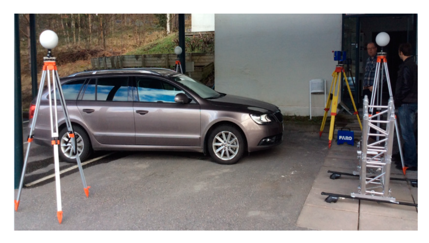
A Skoda Superb 2014 model car was scanned with a Faro Focus3D X330 terrestrial laser scanner (FARO Technologies Inc., Florida, USA), seen in Figure 3 in blue on top of a tripod, obtaining three scans from each side of the vehicle and resulting in a total of six scan stations: two in front of the car, two over the middle section from both sides and two from behind the car. This was done to ensure sufficient overlap between the scans. Five reference spheres were mounted near the vehicle to facilitate the co-registration of individual scans. The scanner mounted on a tripod moves around the car body with six stations, taking approximately five minutes in each station. In total, the scanning time for the car was 30 min. The resulting scans are located in a local Cartesian coordinate system. Figure 3 shows the setup for the car scans. The point cloud of the car is not perfect. Due to the reflective materials of the car windows, the point cloud contains some holes.
3.2. Human Bodies
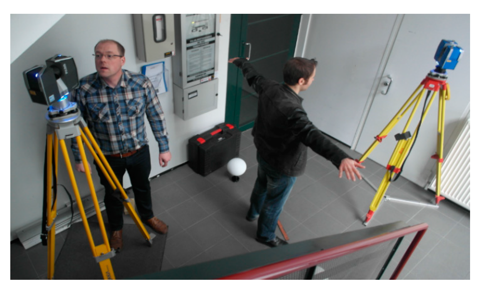
Scanning a human body is not an easy task. Unlike a rigid object, a human body is dynamic, and a small movement of the body can cause failure in the data matching. To ensure the accuracy of the measurement, we simultaneously utilized two static terrestrial Lidars to scan the front and the backside of the human body (FARO Focus3D S120 and X330, respectively). Additionally, to minimize the occlusion from the body, the subject’s two hands were straightened in the horizontal direction at an angle of 90° to the body (Figure 4). After scanning, data from both scanners are registered. Even so, occlusions under the arms and on both sides of the body still exist. The fingers were not properly shown in the resulting data.
3.3. Bookshelf Data Acquisition
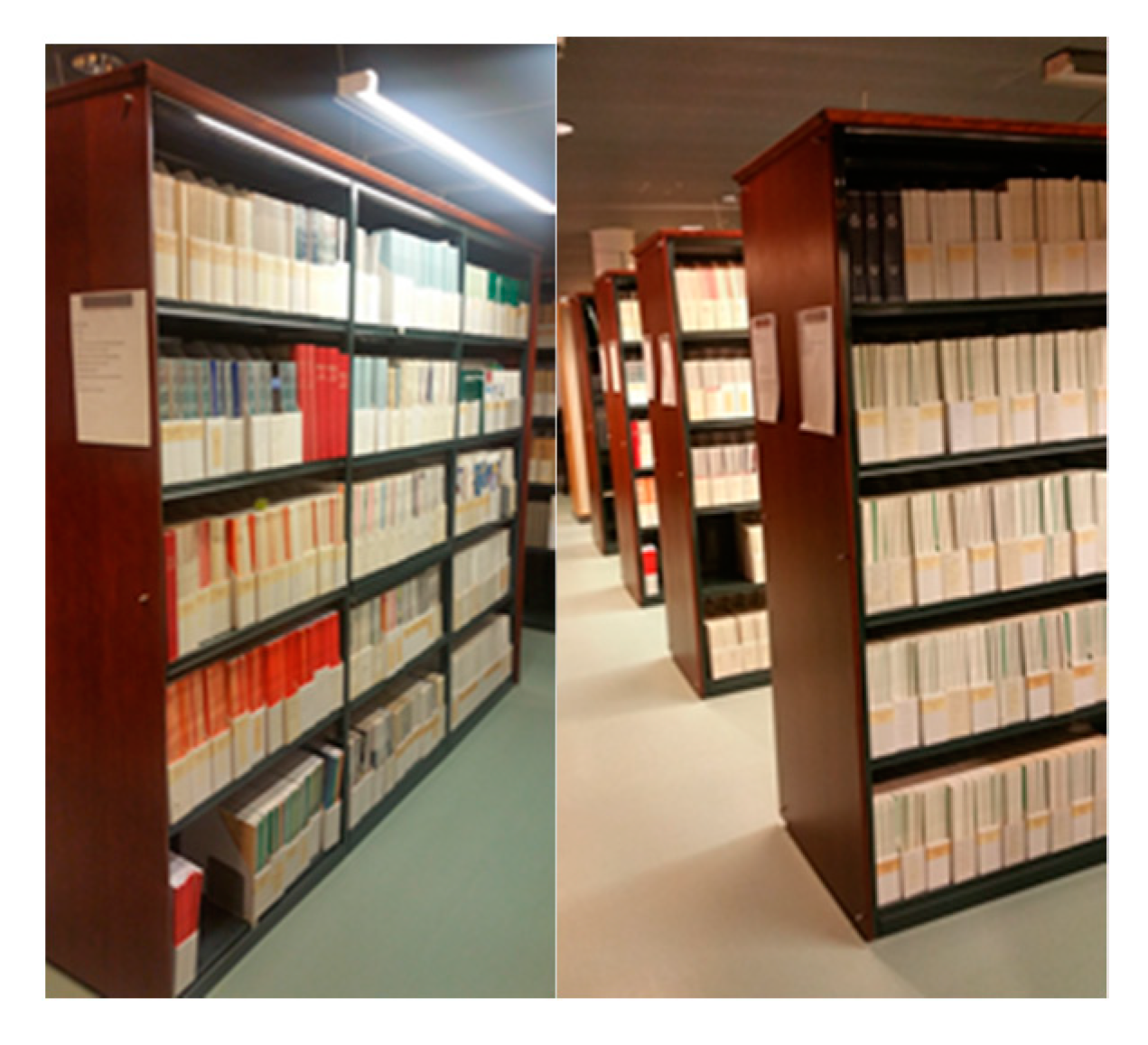
Indoor data were collected by the SLAM-based indoor mobile laser scanning (the FGI SLAMMER) [34]. The FGI SLAMMER was developed by the Finnish Geospatial Research Institute (FGI), Masala, Finland. It is a research platform combining survey-grade sensors with state-of-the-art 2D SLAM algorithms, Karto Open Library and Hector SLAM [34,35]. The FGI SLAMMER consists of two Faro Focus 3D (120S and X330) high-precision laser scanners and a NovAtel SPAN Flexpak6 GNSS receiver with a tactical grade IMU (UIMU-LCI) mounted on a wheeled cart. One scanner is mounted horizontally to collect data for SLAM, and another scanner is mounted vertically for 3D point cloud collection. The test data were from the second floor of the FGI building, around the library area. One bookshelf from the library was chosen as a test object (Figure 4). In the dataset of the bookshelf, there were lights attached on top of it to make the object structure more complicated. In addition, holes exist in the point cloud where there was empty space between books or between books and the shelf.
3.4. Acquisition of Indoor Objects: Two Chairs and A Stool
For 3D digitizing of smaller objects, a Faro Freestyle 3D X hand-held laser scanner was utilized. The instrument operates by projecting a laser pattern (structured light) on the target and photographing it with two infrared cameras and one conventional color camera. The point coordinates are obtained through triangulation, whereas the conventional camera is used to acquire color information for the resulting point cloud. According to the manufacturer, the system is capable of recording up to 88,000 points per second, with a point accuracy of 1 mm [36]. In practice, deviations between 0–2.5 mm have been attained in a comparison with photogrammetric surveys when digitizing geometrically complex cultural heritage artifacts [37].
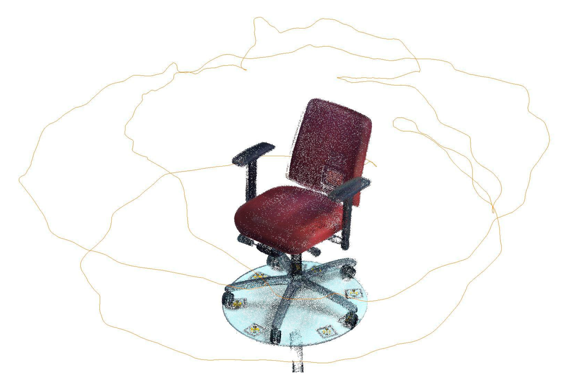
Object scanning was performed by mounting the objects on a flat, white table surface with eight markers of the Faro System installed adjacent to the object, and then circling the object with the scanner (see Figure 5). The targets are automatically detected by the applied Faro Scene software, and assist in co-registering consecutive frames from the instrument. Faro Scene (version 6.0) software was used to post-process the scan data. The scanned point clouds were manually segmented to remove the table surface from the final point clouds.
4. Methods
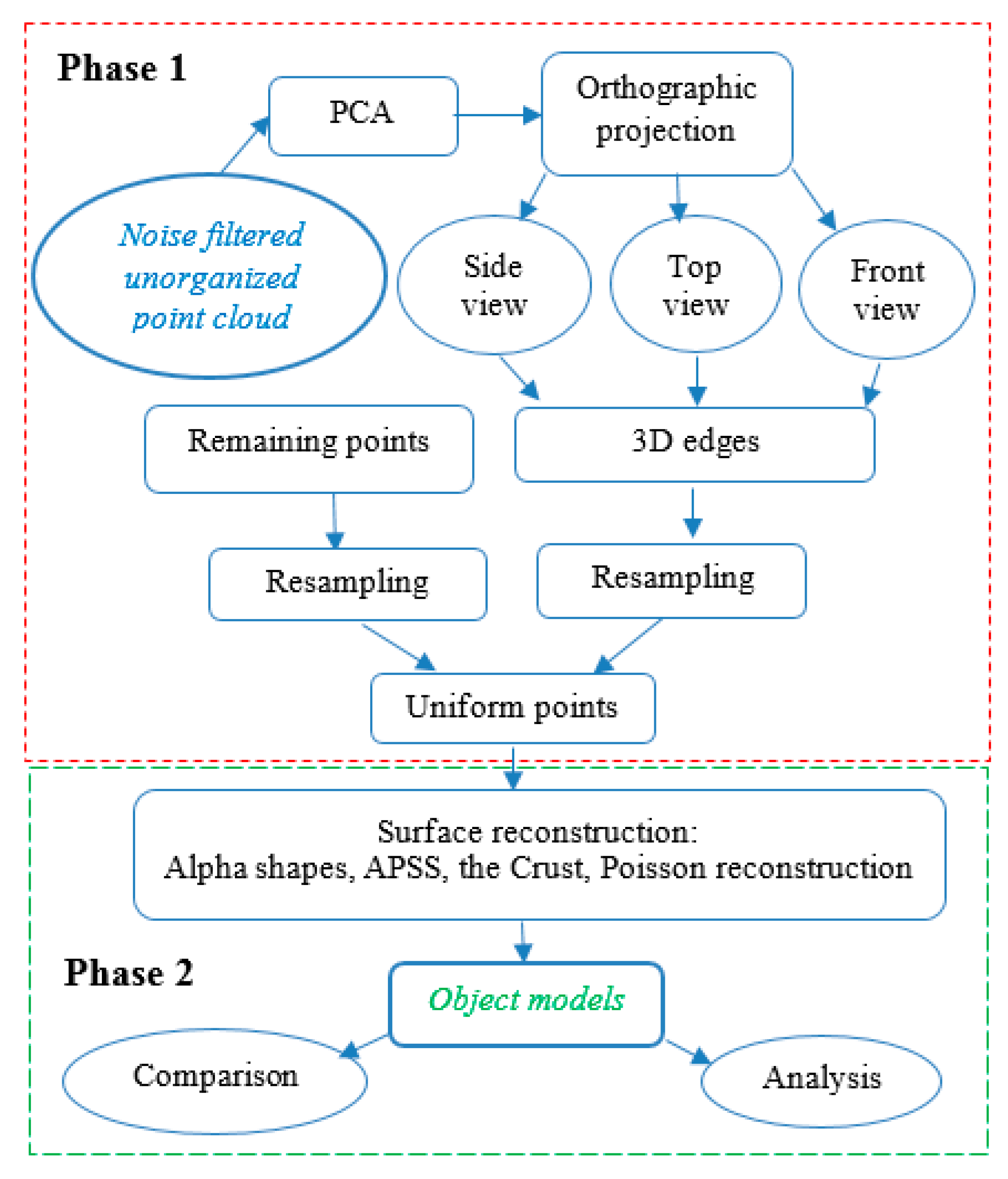
Our method is designed in two phases (see Figure 6). The first phase presents the multi-view point simplification method; the second one is the surface reconstruction with four well-known approaches. The first phase consists of three steps. First, the scanned object was rotated to the orthographic projection by the angle estimated from principal component analysis (PCA). Then, multi-view projection geometry (top-view, front-view and right-side-view) is applied to obtain the edges of the object from each view.
These edge points are merged to produce the three dimensional (3D) edges of the object. Thus, the least important points are separated from the point cloud. Next, a grid-based resampling method is applied to both the key points and the remaining points with different grid sizes to acquire highly accurate and uniform points. In the second phase, the objects are reconstructed by the well-known methods: Alpha shapes, the Crust, Algebraic point set surfaces (APSS), Marching cubes and screened Poisson reconstruction (SPR). The effects of points’ density and quantity on surface reconstruction are investigated. Different reconstruction methods’ handlings of the data imperfections are studied.
4.1. Phase 1: Point Simplification
4.1.1. PCA of the Objects
This method is developed for highly dense point clouds. Prior to the point simplification, the point cloud needs to be segmented into individual objects with the noise removed according to its spatial distribution. The terrestrial laser scanner is operated in a local coordinate system, which is not necessary to produce orthogonal views of the object. Multi-view projection geometry for 3D edge acquisition needs to be in orthogonal projection, so that the key characteristics of an object can be obtained. Therefore, principal component analysis (PCA) for each object needs to be estimated to rotate the object to its orthogonal projection.
PCA is an eigenvector-based multivariate analysis. It utilizes an orthographic transformation method to obtain several sets of linearly-uncorrelated components. For example, a set of point cloud data consists of x, y and z coordinates. A transformation results in three principal components. The first principal component exhibits the axis of the largest possible variance by the elements of the first column of the eigenvalues.
Each succeeding component in turn has the highest variance possible under the constraint that it is orthogonal to the preceding components. This has to satisfy the following equations:
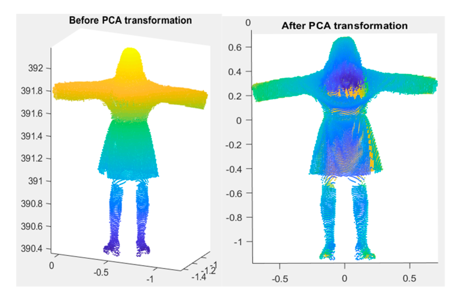
where U is the unit vector of the first weighted component, in X, and each row represents different observations, while each column presents different features. Figure 7 explains the reason why we need to use an orthographic view. In the left image, a set of point clouds of a human body was scanned with a static terrestrial Lidar. It is in a sensor-centered local coordinate system. The origin point of the data varies when the scanner starts in a different position. Therefore, it is not necessary for the data to be in orthographic view. By a PCA estimate, the first main component, that is, the first column of eigenvalues, represents the primary direction of the data in an orthographic projection. The left image of Figure 7 is the original data in a non-orthographic view. The right image shows data after the PCA transformation, which exhibits a clear contour of the scanned human in the orthographic view.
4.1.2. Object 2D Projection
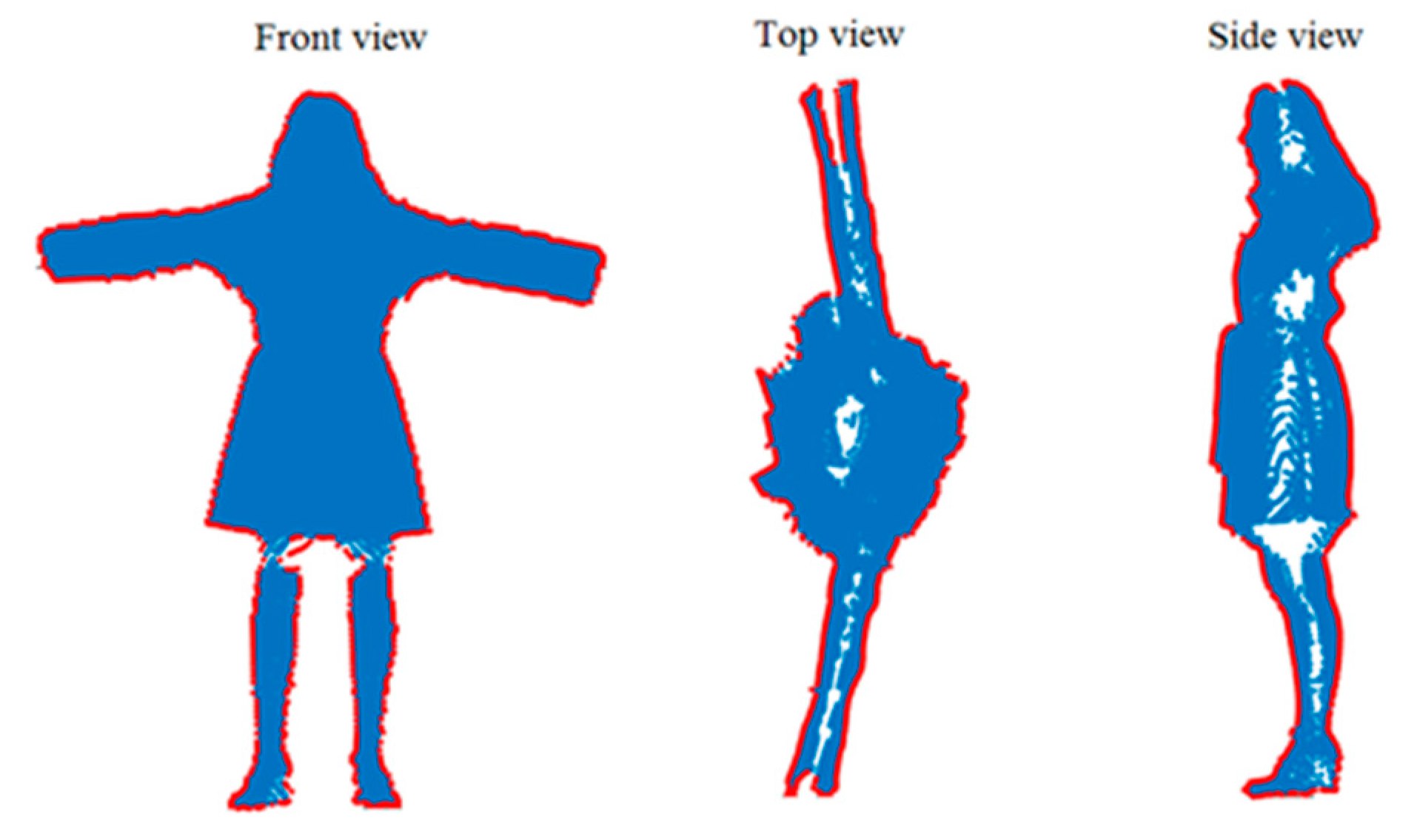
After the transformation of the first component of PCA, the new point cloud of an object is projected onto three orthographic planes: xy, xz and yz. In each 2D projection, the boundary of the object is estimated. A point is a boundary point only if it belongs to both the closure of the dataset and the closure of its complement. If p ϵ s & p ϵ then p ϵ b, where s is a point set; b is a boundary; p is a point; is the complement of the dataset s. Figure 8 shows three 2D boundaries of the orthogonal projections. The 3D edges are achieved by merging the 2D boundaries.
4.1.3. Edge Points Resampling
The laser scanning typically produces very dense point clouds, especially from ground-based terrestrial Lidar. The scan frequency can produce up to millions of points/second. The density is a few hundred points/m2. The point distance on an edge, which we obtained from previous steps, is at the level of millimeters. Furthermore, the edge points usually appear in a zigzag pattern, which is not visually pleasing for the follow-up work (such as measurement or visualization). Therefore, the edge points need to be resampled by a grid filter. The grid size can be selected so that high accuracy and uniform resampled points can be simultaneously achieved. In our case, we chose a grid size of 0.001 m (one millimeter).
4.1.4. Resampling of the Remaining Points
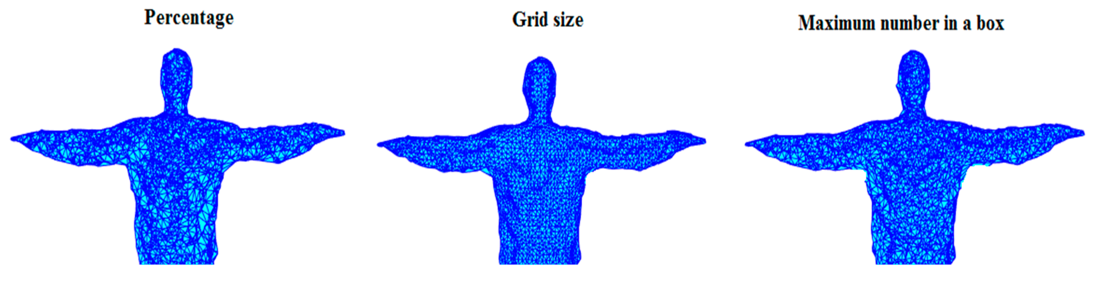
After 3D edge extraction, the remaining points, i.e., points that do not belong to the edge points, are resampled. Usually, these points are the least important because the edge points determine the shape of an object and appear in places where the shape has local contouring. Therefore, these points are resampled based on two principles: one is to keep the geometry at a certain level of detail; another is to achieve a regular point distribution so that the resulting meshes are visually pleasing. There are different resampling methods, such as percentage-based resampling, grid-based resampling and non-uniform resampling.
- Percentage-based resamplingA random resampling method needs to specify the percentage of reduced points. The points are randomly selected from the original points, without replacement. The advantage is its high computational efficiency.
- Grid/box-based resamplingThe grid-based resampling method selects points using a fixed size grid, retaining a single point in each cell. Replacement or interpolation is needed in this case. The advantage of this method is that, after resampling, the points are distributed evenly over the shape surface.
- Number of points in a box resampling (also called non-uniform resampling)In this method, the points are located in cubes. The maximum number of points within a cube is specified. The resampling is conducted by selecting a certain number of points in a cube using the applied criteria/method.
By the above resampling methods, we may define what percentage of input points needs to be reserved, or we may define a grid size for sampling, or we may determine the maximum number of points in a cube.
An experiment has been implemented using different resampling methods. The parameters for these methods were selected so that the number of output points are at similar levels. For example, in Figure 9, we chose a percentage of 20, that is, the number of output points is 20% of the input points, which is 4150 points in this case. In the case of the grid method, we select grid size = 0.0233, in which the number of resulting points is 4158; when the maximum number of points in a cube is eight, the resulting number of points is 4096, which is quite close to the other numbers. However, even with the similar numbers of points, the meshes constructed from these points are quite different. The meshes from the grid-based resampling visually exhibit the best result: continuous and evenly-distributed points.
Therefore, we utilize the grid-based resampling method to reduce the points. To test how point density affects the surface reconstruction, we utilize three grid sizes to filter the remaining points: 0.01 m, 0.02 m and 0.05 m (one, two and five centimeters). After resampling, each point set is merged with the resampled edge points. Thus, each object has four datasets for surface reconstruction, including the original points.
4.2. Phase 2: Surface Reconstruction
In this paper, we tested four well-known surface reconstruction methods: Alpha shapes, APSS, the Crust and SPR. Alpha shapes, APSS and SPR were implemented by Meshlab [38], which was developed by the ISTI-CNR research center (Pisa, Italia). MeshLab is free and open-source software. The sources are from the Visual Computing Lab, which is supported by the Visualization and Computer Graphics Library (VCG) and distributed under the GPL 3.0 Licensing Scheme [38]. The Crust method was performed by MATLAB [39], which is a mathematical computing software for data analysis, algorithm development and model creation. It is developed by MathWorks (Massachusetts, USA).
The point clouds obtained from phase 1 were used for surface reconstruction by the above four methods. We compare and analyze the reconstruction results from i) the original points and the uniform points; and ii) the resampled points with different densities, by their runtime and capacity to handle data imperfection (especially in hole filling). The applicability of these surface reconstruction methods is addressed.
4.3. The Method for Assessing Point Simplification
We employed the standard deviation (SD) to measure the deviation:
where Yt is the distance from point t in the compared point cloud to its nearest neighbor in reference point cloud. is the mean distance. t = 1, 2, 3, …, n and n is the number of points.
5. Results
Test targets/data were selected by their manifold characteristics: different surface materials, different geometric complexities, rigid objects and vivid human bodies. They were scanned by three types of systems: static, mobile and hand-held scanners. This indicates that point densities and the completeness of the data vary when scanned by different systems. In the phase of the point simplification, the eight measured targets/objects, each with four datasets (one original point set and three resampled point sets), yielded 32 total datasets. The runtime and the point reduction were evaluated. In the phase of the surface reconstruction, the 32 datasets from phase 1 and the four reconstruction methods resulted in a total of 128 reconstruction results.
5.1. Results from Phase 1
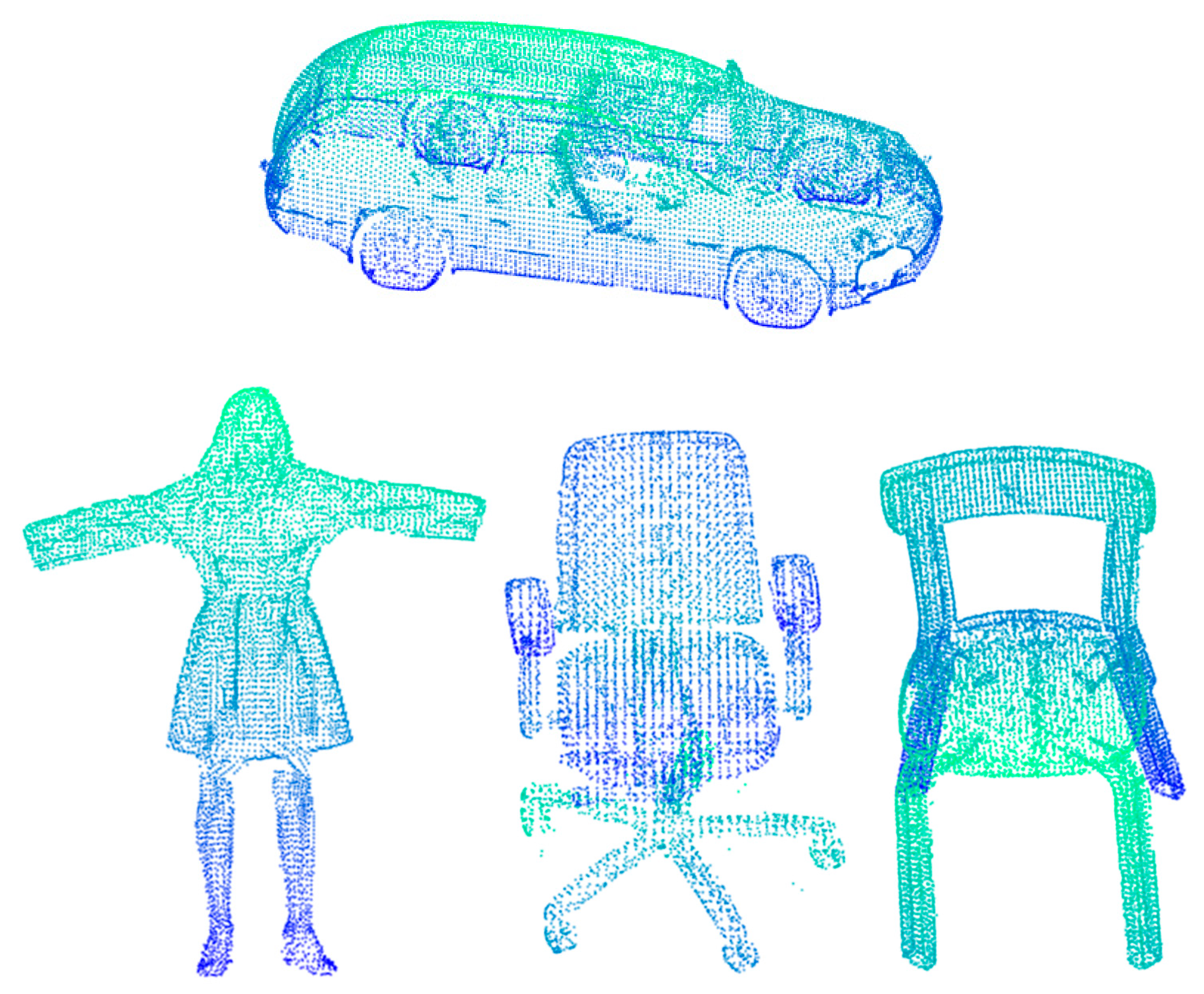
In this phase, point clouds from the eight targets were simplified and made uniform. The edge points were resampled with a grid size of 0.001 m for the edges from all datasets so that uniform edge points were achieved. The remaining points were resampled with the grid sizes of 0.01 m, 0.02 m and 0.05 m. The resulting data are a combination of the resampled edge points and the resampled remaining points. Among these point clouds, the original point cloud of the car contains more than five million points. After the implementation of our method with the resampling sizes of 0.01 m, 0.02 m and 0.05 m for the least important points, 94.032%, 98.428% and 99.671% of points were reduced, respectively. Figure 10 exhibits a close view of the simplified and uniform points taken from the examples of the car, the human body and the chairs. All results from phase 1 are shown in Table 2. From Table 2, it can be seen that, due to the preserved edges, the simplified objects retain the important features in spite of the resampling sizes. In addition, the simplified points are evenly distributed and visually pleasant.
Upper: An example of the car with the point reduction of 99.671%; Lower: the resampled points of a human body and the chairs.
Table 3 presents the number of points of the original one and the resampled ones, as well as the percentage of the point reduction. As mentioned above, we used a fixed grid size of 0.001 m for all edge point resampling, while the remaining points were sampled with different sizes. Therefore, for convenience, in the following discussion, the resampling size refers to the sampling of the least important points. In the case of resampling with a grid size of 0.01 m, there was a big variation in the point reduction: from 28.573% to 94.032%. Taking the example of the human bodies, only approximately 30% of the points were dropped. The average percentage of reduction with the resampling grid size of 0.01 m is 63.362%. In the case of the sampling grid size of 0.05 m, the percentage of reduction in all datasets varies from 83.149% to 99.671%. For the car points, after sampling with a grid size of 0.05 m, only 0.329% of the original points remained. However, it still exhibits the clear characteristics of the target. In the case of the grid size of 0.02 m, the average percentage of reduction is 84.063%. It was observed that the use of approximately 16% of the original data (with 0.02-m internal point resampling) can achieve very realistic results.
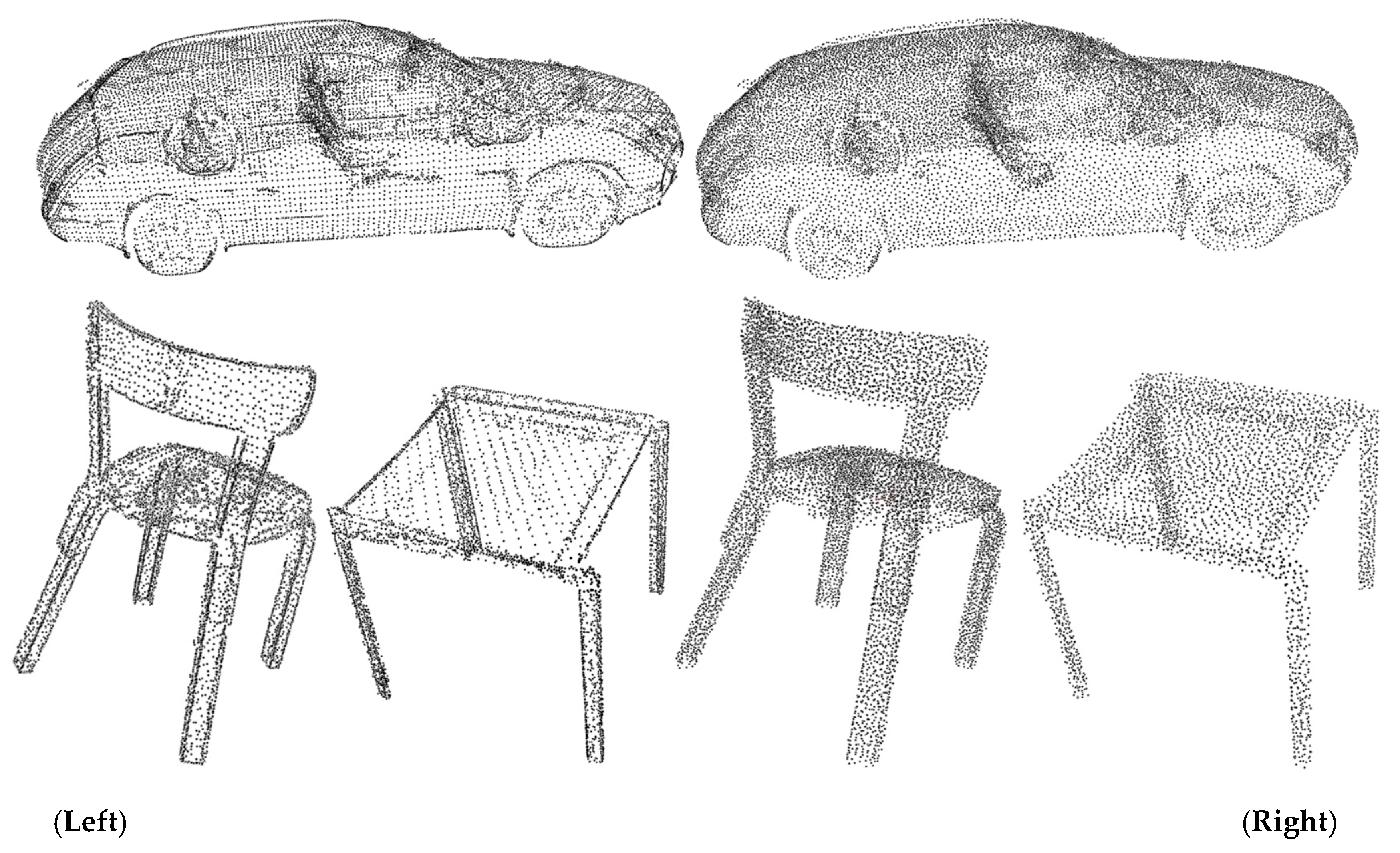
We compared our method with the well-known constrained Poisson disk sampling method by resampling the data to the same amount of points. The car and the chair points were sampled by the Poisson method shown, resulting in the right images of Figure 11. The left images are from our method. It can be seen that our method enhances the visua1 effect.
5.2. Assessment of Phase 1
The point simplification was evaluated by estimating the standard deviation of the resulting points. These resulting points consist of the resampled edge points and the resampled remaining points. We used a grid size of 0.001 m to resample all edge points. For the remaining points, we adopted three different grid sizes: 0.01 m, 0.02 m and 0.05 m. Thus, the results from 24 datasets were evaluated. The assessment was run on a laptop: Dell (Texas, USA) Precision model 7510 (32 GB of RAM and a 2.70-GHz CPU) with the Windows 7 operating system in the MATLAB (MathWorks, 2018) environment.
Table 4 shows the result of the assessment. From the results, it can be seen that the standard deviation rises as the grid size increases in the cases of the grid size of 0.01 m and 0.02 m. However, a ‘surprising’ result occurs when the grid size varies from 0.02 m to 0.05 m. We expect that the standard deviation from data with 0.02-m grid resampling should be smaller than that from 0.05-m resampling. However, this is not the case. The edge points almost retain their original accuracy (with very small grid resampling), especially when the number of edge points is greater than the number of remaining points.
Thus, the average error rate of the entire dataset decreased. In the case of ‘Human1,’ the number of edges is 2064. When grid = 0.05 m, the number of remaining points is only 951, which is much less than the number of edge points. Thus, as long as those 2064 edge points remain correct, the average deviation does not necessarily rise. Taking the example of the bookshelf (BS), the number of remaining points (10,647) is much greater than the number of edge points (3233). Thus, the standard deviation (std) in the case of 0.05-m grid down-sampling is greater than that in the 0.02-m grid down-sampling. The result shows that the separation between the edge points and the remaining points can well control the accuracy. This is one of the advantages of our method.
5.3. Result of Phase 2
We exploited both the original points and the simplified points for surface reconstruction. Four reconstruction methods, i.e., Alpha shapes, APSS, the Crust and SPR, were applied. They were conducted by Meshlab and MATLAB. 128 models from 32 datasets with four methods were obtained. From the above assessment, the average point reduction with the resample size of 0.01 m was 63.36%. The difference in reconstruction results from the original points and from the simplified points varies with the methods. However, all methods are beneficial from the point simplification for the reduction of running time (see Table 5). Alpha shapes reconstruction with uniform points produces smoother meshes and is visually more pleasant. For the Crust method, the number of meshes from the simplified points was much less than that from the original points. Except for the method of Alpha shapes, the other reconstruction methods rearranged (including adding or removing) the input points for meshing.
When surfaces were reconstructed from the low, dense points, the main benefits were to save storage space and be convenient for the following up work, e.g., rendering. When the same parameters are used, in the method of the Crust and SPR, fewer points produce fewer meshes. However, in the method of APSS, the opposite is true. In the method of Alpha shapes, it varies with different objects. For example, during the human1 reconstruction, 32,034 meshes were produced from the original data with 21,041 points, while 89,868 meshes were produced from 14,682 resampled points. For the reconstruction of human3, it was the same as with the method of the Alpha shapes. From Table 5, it can also be seen that half of the reconstruction methods failed when the number of points was huge (more than five million) in the case of the car. Therefore, point simplification is necessary when surfaces are reconstructed from such huge datasets.
Data imperfection from data acquisition is hard to avoid when reflective materials and occlusions exist in a scene. Some reconstruction methods are able to fill the holes, for instance, SPR and the Crust. Although there were many holes presented in the data of human bodies, the reconstruction results from SPR were visually outcompeted: smooth and no holes.
However, the method of SPR failed in the reconstruction of thin parts of the objects, e.g., chair legs and lights on top of the bookshelf. Regarding the fidelity, efficiency and capacity of dealing with diverse data with and without holes, in total, the Crust performs the best. One of the advantages of the APSS is that the reconstructed models express the geometry in detail. However, the reconstruction results were awfully unsmoothed. The Alpha shapes successfully reconstructed chairs and the stool for all resampling sizes. However, many holes remained from the reconstruction of human bodies (see Table 6).
5.4. Recommendation of Surface Reconstruction Methods
The reconstruction methods of Alpha shapes, APSS, the Crust and SPR for diverse objects with different densities of points and data imperfections have been studied. The Car data contain more than five million points and have data imperfections (reflections from metal and glassy windows). Two methods (Alpha shapes and APSS) failed in reconstruction from original data, but they all work for simplified points. Due to the capacity of hole-filling in the methods of the Crust and SPR, they both can be used for car reconstruction. However, the reconstruction results vary with changes in point density. It was shown that dense points were not necessary to achieve good reconstruction results. From Figure 12, it can be seen that one tire was missing during the reconstruction from the denser points, but they were reconstructed from the sparser points. A similar case also happens in the method of APSS. For the SPR, the reconstruction from sparse points loses the details, and the results were also over-smoothed in reconstruction from both the original points and the sparse data.
Therefore, the results were not stable as the number of points decreases. We would recommend that the SPR method can be utilized for car reconstruction only at a certain level of point density. For the Crust method, relatively sparse data might achieve a better result.
Regarding human body reconstruction, the Crust and the SPR are recommended due to their capacity to deal with the data imperfections. The method of APSS produced the clearest details of the face characteristics. If the data scanned from a human body were dense and complete (no holes under the arms and from the sides), the methods of the Alpha shape and the APSS would also be suitable for its reconstruction. The Bookshelf can be reconstructed by most of the methods. Without the two lights attached to the top of the bookshelf, the SPR method should also work well. Data of the stool and the chairs were complete. The Alpha shapes and the Crust can produce good results, but the results from the APSS were extremely unsmoothed, and those from the SPR lost fidelity as the number of points decreased. Table 7 shows the recommendations for the methods used for different objects’ reconstruction. The recommendation is based on our test data with or without data imperfections.
6. Discussion and Future Work
In this paper, a Multi-view projection method was proposed to obtain 3D edges. Three-view projections were applied. However, in 3D modeling software, there are six standard drawing views: top view, front view, left view, back view, right view and bottom view. To verify the effectiveness of using three orthographic views to represent an object’s 3D shape, we conducted an experiment. We extracted the boundaries of objects from six orthographic views, merged these boundaries, and removed the duplicate points. The boundaries from the six views were compared with those from the three views. It turned out that both produced the same edge points.
The Multi-view projection method can successfully extract the external boundaries of the objects. When objects contain complex structures, e.g., multiple internal edges, or encounter occlusions from the three projections, internal details might not be fully presented.
There is a need to simplify the points prior to surface reconstruction when objects contain a large number of points, e.g., five million points in the car dataset. Without the point simplification, the reconstruction methods might not work. For a small object, the benefits of point simplification are to reduce the surface reconstruction time and conserve data storage. The benefit of the point uniformity prior to the reconstruction is to achieve visually pleasing results. By using our method, objects were visually enhanced. The proposed method is applicable and operable in practice.
It is necessary to continuously develop surface reconstruction methods to improve their capacity to reconstruct diverse objects. The main concerns for future development are i) how to deal with data imperfections; ii) how to ascertain the proper level of smoothing; iii) how to achieve a model with geometric details and fidelity; iv) how to improve the capacity to reconstruct diverse objects.
7. Conclusions
In this paper, we utilized two static terrestrial Lidar systems, one trolley-based mobile terrestrial Lidar system, and one handheld Lidar system, for data acquisition from dynamic and rigid targets. Extremely dense point clouds from eight targets were obtained. The work was divided into two phases. In the first phase, we utilized PCA and a Multi-view projection method to separate 3D edges from the least important points. 3D edges were resampled with a small grid, while the least important points were resampled with a large grid. Thus, the accuracy of the simplified points remained high. Point reduction up to 99.371% with a standard deviation of 0.2 cm was achieved. With the grid resampling, the resultant points are uniform. Our point simplification method was compared to the well-known constrained Poisson disk sampling method. The results from our method enhanced the visual expression. In the second phase, four well-known surface reconstruction methods (Alpha shape, APSS, the Crust and SPR) were employed to reconstruct the object surfaces from the original points and the simplified points with different resampling densities. A total of 128 surfaces of the targets were reconstructed. The difference between the reconstructions from the original points and from the simplified points revealed that resampling with a high density was beneficial in that it reduced runtime while still achieving similar results. For a large number of points, point simplification became necessary to ensure that the reconstruction methods work normally. When using simplified points of different densities for surface reconstruction, it was found that, in the method of APSS, the number of input points is inversely proportional to the number of output meshes, whereas the methods of the Crust and the SPR exhibited the opposite trend. The Crust method deals well with different densities of data. SPR deals the best with data imperfection. Alpha shapes work well if the data are complete. The APSS provided the most details of object geometry. Recommendations and concerns for future development were addressed.
In the future, surface reconstruction methods may focus on improving the capacity to reconstruct diverse objects, maintaining a balance between smoothing and preserving geometric details, and extending the capacity to handle data imperfections.
Author Contributions
Data curation, K.A., V.J.-P., and T.T.; Funding acquisition, H.J., K.H. and H.H.; Investigation, Z.L.; Methodology, Z.L.; Project administration, K.H.; Resources, H.J. and H.H.; Writing—original draft, Z.L.; Writing–review & editing: H.J., K.A., and V.J.-P.
Funding
This research was funded by the Academy of Finland for their support of the Center of Excellence in Laser Scanning Research (CoE-LaSR; 272195) and Strategic Research Council at the Academy of Finland is acknowledged for financial support for project “Competence Based Growth Through Integrated Disruptive Technologies of 3D Digitalization, Robotics, Geospatial Information and Image Processing/Computing-Point Cloud Ecosystem (293389/314312)”.
Acknowledgments
Many thanks to Heli Honkanen, Teemu Hakala and Nataliya Zubko’s participation during the data acquisition.
Conflicts of Interest
The authors declare no conflict of interest.
References
- Berger, M.; Tagliasacchi, A.; Seversky, L.; Alliez, P.; Levine, J.; Sharf, A.; Silva, C. State of the Art in Surface Reconstruction from Point Clouds, Eurographics 2014-State of the Art Reports; Strasbourg, France, 2014; 161–185.
- Edelsbrunner, H.; Mucke, E.P. Three-Dimensional alpha shapes. ACM Trans. Graph. 1994, 13, 43–72. [Google Scholar] [CrossRef]
- Bernardini, F.; Mittleman, J.; Rushmeier, H.; Silva, C.; Taubin, G. The ball-pivoting algorithm for surface reconstruction. IEEE Trans. Vis. Comput. Graph. 1999, 5, 349–359. [Google Scholar] [CrossRef]
- Amenta, N.; Choi, S.; Kolluri, R.K. The power crust, unions of balls, and the medial axis transform. Comput. Geom. 2001, 19, 127–153. [Google Scholar] [CrossRef]
- Giaccari, L. Surface Reconstruction from Scattered Point Cloud. MATLAB Central. July 2017. Available online: https://se.mathworks.com/matlabcentral/fileexchange/63730-surface-reconstruction-from-scattered-points-cloud (accessed on 8 November 2018).
- Guennebaud, G.; Gross, M. Algebraic Point Set Surfaces. In Proceedings of the ACM SIGGRAPH 2007 Papers, San Diego, CA, USA, 05–09 August 2007; ACM SIGGRAPH. [Google Scholar]
- Cohen-Steiner, D.; Alliez, P.; Desbrun, M. Variational shape approximation. ACM Trans. Graph. 2004, 23, 905–914. [Google Scholar] [CrossRef]
- Song, H.; Feng, H.-Y. A progressive point cloud simplification algorithm with preserved sharp edge data. Int. J. Adv. Manuf. Technol. 2009, 45, 583–592. [Google Scholar] [CrossRef]
- Leal, N.; Leal, E.; German, S.-T. A linear programming approach for 3D point cloud simplification. IAENG Int. J. Comput. Sci. 2017, 44, 60–67. [Google Scholar]
- Chen, S.; Tian, D.; Feng, C.; Vetro, A.; Kovačević, J. Fast resampling of three-dimensional point clouds via graphs. IEEE Trans. Signal Process. 2017, 66, 666–681. [Google Scholar] [CrossRef]
- Qi, J.; Hu, W.; Guo, Z. Feature preserving and uniformity-controllable point cloud simplification on graph. In Proceedings of the 2019 IEEE International Conference on Multimedia and Expo (ICME), Shanghai, China, 8–12 July 2019; pp. 284–289. [Google Scholar]
- Hastings, W.K. Monte Carlo sampling methods using Markov chains and their applications. Biometrika 1970, 57, 97–109. [Google Scholar] [CrossRef]
- Corsini, M.; Cignoni, P.; Scopigno, R. Efficient and flexible sampling with blue noise properties of triangular meshes. IEEE Trans. Vis. Comput. Graph. 2012, 18, 914–924. [Google Scholar] [CrossRef]
- Floater, M.S. Parametrization and smooth approximation of surface triangulations. Comput. Aided Geom. Des. 1997, 14, 231–250. [Google Scholar] [CrossRef]
- Floater, M.S.; Reimers, M. Meshless parameterization and surface reconstruction. Comput. Aided Geom. Des. 2001, 18, 77–92. [Google Scholar] [CrossRef]
- Gal, R.; Shamir, A.; Hassner, T.; Pauly, M.; Cohen-Or, D. Surface reconstruction using local shape priors. In Proceedings of the Fifth Eurographics Symposium on Geometry Processing (SGP), Barcelona, Spain, 4–6 July 2007; pp. 253–262. [Google Scholar]
- Lafarge, F.; Alliez, P. Surface reconstruction through point set structuring. Comput. Graph. Forum. 2013, 32, 225–234. [Google Scholar] [CrossRef]
- Lorensen, W.E.; Cline, H.E. Marching cubes: A high resolution 3D surface construction algorithm. Comput. Graph. 1987, 21, 163–170. [Google Scholar] [CrossRef]
- Newman, T.S.; Yi, H. A survey of the marching cubes algorithm. Comput. Graph. 2006, 30, 854–879. [Google Scholar] [CrossRef]
- Amenta, N.; Choi, S.; Dey, T.K.; Leekha, N. A simple algorithm for homeomorphic surface reconstruction. Int. J. Comput. Geom. Appl. 2002, 12, 125–141. [Google Scholar] [CrossRef]
- Dey, T.K.; Goswami, S. Provable surface reconstruction from noisy samples. Comput. Geom. 2006, 35, 124–141. [Google Scholar] [CrossRef]
- Dey, T.K.; Dyer, R.; Wang, L. Localized cocone surface reconstruction. Comput. Graph. 2011, 35, 483–491. [Google Scholar] [CrossRef]
- Kazhdan, M.; Bolitho, M.; Hoppe, H. Poisson surface reconstruction. In Proceedings of the Fourth Eurographics Symposium on Geometry Processing, Aire-la-Ville, Switzerland, 26–18 June 2006. [Google Scholar]
- Kazhdan, M.; Hoppe, H. Screened poisson surface reconstruction. ACM Trans. Graph. 2013, 32, 29. [Google Scholar] [CrossRef]
- Manson, J.; Petrova, G.; Schaefer, S. Streaming surface reconstruction using wavelets. In Computer Graphics Forum; Blackwell Publishing Ltd.: Oxford, UK, 2008; pp. 1411–1420. [Google Scholar]
- Treece, G.M.; Prager, R.W.; Gee, A.H. Regularised marching tetrahedra: Improved iso-surface extraction. Comput. Graph. 1999, 23, 583–598. [Google Scholar] [CrossRef]
- Ho, C.C.; Wu, F.C.; Chen, B.Y.; Chuang, Y.Y.; Ouhyoung, M. Cubical marching squares: Adaptive feature preserving surface extraction from volume data. In Computer Graphics Forum; Blackwell Publishing Inc.: Oxford, UK; Boston, MA, USA, 2005; pp. 537–545. [Google Scholar]
- Roy, S.; Augustine, P. Comparative Study of Marching Cubes Algorithms for the Conversion of 2D image to 3D. Int. J. Comput. Intell. Res. 2017, 13, 327–337. [Google Scholar]
- Bernardini, F.; Bajaj, C.L. Sampling and Reconstructing Manifolds Using Alpha-Shapes; Technical Reports in Department of Computer Science, Purdue University: West Lafayette, IN, USA, 1997; Paper 1350. [Google Scholar]
- Soltani, A.; Huang, H.; Wu, J.; Kulkarni, T.D.; Tenenbaum, J.B. Synthesizing 3D shapes via modeling multi-view depth maps and silhouettes with deep generative networks. In Proceedings of the IEEE Conference on Computer Vision and Pattern Recognition, Honolulu, HI, USA, 21–26 July 2017; pp. 1511–1519. [Google Scholar]
- Han, X.-F.; Laga, H.; Bennamoun, M. Image-based 3D object reconstruction: State-of-the-art and trends in the deep learning era. arXiv 2019, arXiv:1906.065432019. [Google Scholar]
- Wiemann, T.; Annuth, H.; Lingemann, K.; Hertzberg, J. An extended evaluation of open source surface reconstruction software for robotic applications. J. Intell. Robot. Syst. 2015, 77, 149–170. [Google Scholar] [CrossRef]
- Khatamian, A.; Arabnia, H.R. Survey on 3D surface reconstruction. J. Inform. Process. Syst. 2016, 12, 338–357. [Google Scholar]
- Kaijaluoto, R.; Kukko, A.; Hyyppa, J. Precise indoor localization for mobile laser scanner. Int. Arch. Photogramm. Remote Sens. Spat. Inf. Sci. 2015, XL-4/W5, 1–6. [Google Scholar] [CrossRef]
- Lehtola, V.; Kaartinen, H.; Nüchter, A.; Kaijaluoto, R.; Kukko, A.; Litkey, P.; Honkavaara, E.; Rosnell, T.; Vaaja, M.; Virtanen, J.-P. Comparison of the selected state-of-the-art 3D indoor scanning and point cloud generation methods. Remote. Sens. 2017, 9, 796. [Google Scholar] [CrossRef]
- FARO. Faro Freestyle 3D X Scanner. 2015. Available online: https://farosocial.blob.core.windows.net/share/hardware/freestylex/freestyle3dx_techsheet.pdf (accessed on 9 November 2008).
- Lachat, E.; Landes, T.; Grussenmeyer, P. Performance investigation of a handheld 3D scanner to define good practices for small artefact 3D modeling. Int. Arch. Photogramm. Remote Sens. Spat. Inf. Sci. 2017, 42, 1682–1750. [Google Scholar] [CrossRef] [Green Version]
- MeshLab. MeshLab Description. 2018. Available online: http://www.meshlab.net/ (accessed on 26 February 2019).
- MathWorks. MATLAB. 2018. Available online: https://www.mathworks.com/products/matlab.html (accessed on 27 February 2019).
Figure 1.
Point simplification and surface reconstruction with different algorithms. (a): point simplification with feature preservation and uniform resampling; (b): surface reconstruction by different methods: Alpha shapes, algebraic point set surfaces (APSS), the Crust, and Screened Poisson reconstruction (SPR).

Figure 2.
Photo of the scene of the bookshelf in a library.

Figure 3.
The car was scanned by a FARO Focus3D X330 terrestrial laser scanner. The scanner was mounted on the yellow tripod, seen near the right. Three of the five white reference spheres are also visible.
Figure 3.
The car was scanned by a FARO Focus3D X330 terrestrial laser scanner. The scanner was mounted on the yellow tripod, seen near the right. Three of the five white reference spheres are also visible.

Figure 4.
The scene of human body acquisition.

Figure 5.
An object point cloud reconstructed with a hand-held scanner shown with the measurement trajectory and automatically detected markers mounted adjacent to the object on the table surface.
Figure 5.
An object point cloud reconstructed with a hand-held scanner shown with the measurement trajectory and automatically detected markers mounted adjacent to the object on the table surface.

Figure 6.
Workflow of the point simplification and surface reconstruction. Two phases: the first phase in the red frame concerns the point simplification; the second phase within the green frame concerns surface reconstruction.
Figure 6.
Workflow of the point simplification and surface reconstruction. Two phases: the first phase in the red frame concerns the point simplification; the second phase within the green frame concerns surface reconstruction.

Figure 7.
The difference between before principal component analysis (PCA) transformation and after PCA transformation for human body scanning data. (See the axis for the difference). Because both images are in local coordinate systems, there are no units for the axes.
Figure 7.
The difference between before principal component analysis (PCA) transformation and after PCA transformation for human body scanning data. (See the axis for the difference). Because both images are in local coordinate systems, there are no units for the axes.

Figure 8.
Three 2D projections: Front, top and side.

Figure 9.
Different resampling methods.

Figure 10.
A close view of the results of the point simplification and uniformity.

Figure 11.
Comparing our method with the Poisson sampling method. (Left): our method; (Right): Poisson sampling method.
Figure 11.
Comparing our method with the Poisson sampling method. (Left): our method; (Right): Poisson sampling method.

Figure 12.
Car reconstruction from different point densities by the methods of the Crust and SPR. Left two images: the Crust with the resampling points of 0.01 m and 0.05 m, respectively; Right three images: the SPR with the original points and the resampling points of 0.01 m and 0.05 m, respectively.


Table 1.
Comparison of the evaluated methods with respect to the considered criteria ranging from +++ (very good) to --- (very poor) (From Wiemann et al. [32]).
Table 1.
Comparison of the evaluated methods with respect to the considered criteria ranging from +++ (very good) to --- (very poor) (From Wiemann et al. [32]).
| Open Geometry | Closed Geometry | Sharp Features | Topological Correctness | Noise Robustness | Run Time | |
|---|---|---|---|---|---|---|
| Poisson Reconstruction | -- | +++ | - | ++ | +++ | o |
| Ball Pivoting | o | o | o | -- | --- | - |
| Alpha Shapes | o | o | o | -- | --- | - |
| APSS Marching Cubes | ++ | ++ | o | ++ | o | - |
| LVR Planar Marching Cubes | +++ | ++ | ++ | ++ | ++ | + |
| Kinect Fusion | ++ | ++ | -- | --- | +++ | +++ |
Table 2.
The results of point simplification.
| Original Points | Simplification1 | Simplification2 | Simplification3 |
|---|---|---|---|
 |  |  |  |
 |  |  |  |
 |  |  |  |
 |  |  |  |
 |  |  |  |
 |  |  |  |
 |  |  |  |
 |  |  |  |
Table 3.
The number of points and the percentage of reduction in the number of points.
| Object | Number of: Original Points | The Number of Points (Edge Points + Internal Points) | Percentage of Reduction (%) | ||||
|---|---|---|---|---|---|---|---|
| Grid = 0.01 (m) * | Grid = 0.02 (m) * | Grid = 0.05 (m) * | Grid = 0.01 (m) * | Grid = 0.02 (m) * | Grid = 0.05 (m) * | ||
| Car | 5,549,404 | 331,207 | 87,213 | 18,249 | 94.032 | 98.428 | 99.671 |
| Human1 | 21,041 | 14,682 | 6551 | 3015 | 30.222 | 68.865 | 85.671 |
| Human2 | 16,848 | 12,034 | 5694 | 2839 | 28.573 | 66.204 | 83.149 |
| Human3 | 23,979 | 16,635 | 7287 | 2995 | 30.627 | 69.611 | 87.510 |
| BS | 252,418 | 145,688 | 57,769 | 13,880 | 42.283 | 77.114 | 94.501 |
| Chair1 | 202,803 | 13,322 | 5724 | 3901 | 93.431 | 97.178 | 98.076 |
| Chair2 | 436,849 | 27,351 | 7472 | 2526 | 93.739 | 98.290 | 99.422 |
| Stool | 146,000 | 8782 | 4649 | 3580 | 93.985 | 96.816 | 97.548 |
| Average | 63.362 | 84.063 | 93.194 | ||||
* ‘grid = 0.01 m, 0.02 m and 0.05 m’ refers to the internal point resampling grid.
Table 4.
Assessment of point simplification.
| Object | NumP: Original Points * | NumP: Edge Points * | Runtime (s) | NumP: Resampled Edge Points Grid = 0.005 m * | Number of Internal Point Resampling | Accuracy in all Points (std) (cm) | ||||
|---|---|---|---|---|---|---|---|---|---|---|
| Grid = 0.01 m | Grid = 0.02 m | Grid = 0.05 m | Grid = 0.01 m | Grid = 0.02 m | Grid = 0.05 m | |||||
| Car | 5,549,404 | 5785 | 125.45 | 4850 | 326,357 | 82,363 | 13,399 | 0.086 | 0.113 | 0.203 |
| Human1 | 21,041 | 2065 | 0.508 | 2064 | 12,618 | 4487 | 951 | 0.177 | 0.214 | 0.207 |
| Human2 | 16,848 | 2016 | 0.404 | 2016 | 10,018 | 3678 | 823 | 0.173 | 0.218 | 0.195 |
| Human3 | 23,979 | 1928 | 0.538 | 1928 | 14,707 | 5359 | 1067 | 0.179 | 0.229 | 0.262 |
| BS | 252,418 | 3317 | 5.673 | 3233 | 142,455 | 54,536 | 10,647 | 0.156 | 0.227 | 0.389 |
| Chair1 | 202,803 | 4884 | 5.024 | 3585 | 9737 | 2139 | 316 | 0.087 | 0.106 | 0.099 |
| Chair2 | 436,849 | 1927 | 11.82 | 1735 | 25,616 | 5737 | 791 | 0.087 | 0.114 | 0.173 |
| Stool | 146,000 | 5524 | 3.673 | 3385 | 5397 | 1264 | 195 | 0.066 | 0.08 | 0.075 |
| Average | 0.116 | 0.163 | 0.200 | |||||||
* ‘NumP’ refers to the number of points; ‘BS’ is the bookshelf; ‘std’ is the standard deviation; ‘Accuracy in all points’: all points refers to the regular edge points and resampled internal points; grid = 0.01 m, 0.02 m and 0.05 m are the internal point resampling sizes.
Table 5.
Surface reconstruction methods and evaluation.
| Alpha Shape | APSS (Grid Resolution = 500) | Crust | SPR | |||||||||
|---|---|---|---|---|---|---|---|---|---|---|---|---|
| Run Time (s) | Number of Meshes | Hole (Y/N) | Run Time (s) | Number of Meshes * | Hole (Y/N) | Run Time (s) | Number of Meshes | Hole (Y/N) | Run Time (s) | Number of Meshes | Hole (Y/N) | |
| Car_org | failed | failed | 1814.5 | 12,529,297 | N | 11 | 188,088 | N | ||||
| Car_1 | 25.6 | 932,630 | Y | 53.2 | 655,075 | Y | 93.8 | 737,790 | N | 7.8 | 206,516 | N |
| Car_2 | 4.3 | 359,902 | Y | 17.5 | 742,331 | Y | 22.8 | 175,961 | N | 7.4 | 202,206 | N |
| Car_5 | 0.7 | 76,117 | Y | 12.7 | 827,202 | Y | 4.8 | 34,533 | N | 3.3 | 79,684 | N |
| Hu1_org | 3.8 | 32,034 | Y | 8.4 | 339,328 | Y | 5.9 | 45,339 | N | 3.6 | 91,014 | N |
| Hu1_1 | 0.8 | 89,868 | Y | 7.1 | 310,857 | Y | 3.9 | 29,116 | N | 3.5 | 79,142 | N |
| Hu1_2 | 0.2 | 31,409 | Y | 6.3 | 337,071 | Y | 1.9 | 12,919 | N | 1.7 | 27,436 | N |
| Hu1_5 | 0.1 | 9279 | Y | 6.2 | 372,628 | Y | 1.1 | 5948 | N | 1.5 | 20,746 | N |
| Hu2_org | 1.1 | 116,032 | Y | 7.4 | 295,369 | Y | 4.9 | 36,758 | N | 3.2 | 205,132 | N |
| Hu2_1 | 0.7 | 72,574 | Y | 6.1 | 258,619 | Y | 3.4 | 23,747 | N | 2.9 | 80,854 | N |
| Hu2_2 | 0.3 | 28,056 | Y | 6.0 | 282,096 | Y | 1.9 | 11,261 | N | 1.7 | 25,606 | N |
| Hu2_5 | 0.1 | 9544 | Y | 5.8 | 314,521 | Y | 1.0 | 5588 | N | 1.4 | 19,400 | N |
| Hu3_org | 5.1 | 31,124 | Y | 6.7 | 338,799 | Y | 6.5 | 47,814 | N | 3.6 | 90,042 | N |
| Hu3_1 | 0.9 | 82,919 | Y | 6.6 | 339,403 | Y | 4.5 | 33,127 | N | 3.4 | 85,250 | N |
| Hu3_2 | 0.3 | 32,058 | Y | 5.7 | 347,050 | Y | 2.2 | 14,420 | N | 1.7 | 26,622 | N |
| Hu3_5 | 0.1 | 8022 | Y | 5.5 | 359,493 | Y | 0.9 | 5867 | N | 1.4 | 19,868 | N |
| BS_org | 25.3 | 500,103 | Y | 113 | 2,343,075 | Y | 63.9 | 489,601 | Y | 19.1 | 556,746 | N |
| BS_1 | 17.5 | 359,227 | Y | 87.0 | 2,505,295 | Y | 37.4 | 290,048 | Y | 18.3 | 535,830 | N |
| BS_2 | 2.2 | 203,125 | Y | 45.4 | 2,606,712 | Y | 15.0 | 114,724 | Y | 8.5 | 210,352 | N |
| BS_5 | 0.5 | 44,995 | Y | 41.6 | 2,663,567 | Y | 4.1 | 26,523 | Y | 2.8 | 42,560 | N |
| Ch1_org | 7.4 | 174,942 | N | 86.4 | 1,288,477 | N | 8.6 | 452,190 | N | 7.2 | 168,126 | N |
| Chr1_1 | 0.4 | 40,203 | N | 18.2 | 838,936 | N | 4.0 | 27,316 | N | 2.3 | 42,612 | N |
| Ch1_2 | 0.2 | 18,870 | Y | 13.9 | 814,207 | N | 1.8 | 11,280 | N | 2.2 | 32,738 | N |
| Ch1_5 | 0.1 | 11,578 | Y | 12.9 | 803,961 | Y | 1.4 | 7381 | Y | 1.8 | 32,600 | N |
| Ch2_org | 16.3 | 228,214 | N | 148 | 1,813,631 | N | 126 | 869,919 | N | 10.2 | 218,433 | N |
| Ch2_1 | 1.0 | 72,423 | N | 22.4 | 1,082,339 | N | 7.6 | 45,657 | N | 4.4 | 98,350 | N |
| Ch2_2 | 0.3 | 24,359 | Y | 14.9 | 989,877 | N | 2.4 | 11,831 | N | 2.1 | 36,265 | N |
| Ch2_5 | 0.1 | 6799 | Y | 13.9 | 1,162,428 | Y | 1.0 | 4023 | Y | 1.5 | 20,510 | N |
| Stool_org | 5.1 | 189,983 | N | 50.7 | 902,489 | N | 39.7 | 314,142 | N | 7.0 | 187,248 | N |
| Stool_1 | 0.3 | 29,506 | N | 17.5 | 657,254 | N | 2.6 | 17,468 | N | 2.1 | 42,390 | N |
| Stool_2 | 0.2 | 15,257 | Y | 15.6 | 652,582 | N | 1.5 | 9088 | N | 1.8 | 35,644 | N |
| Stool_5 | 0.1 | 12,415 | Y | 15.2 | 620,818 | Y | 1.2 | 6974 | Y | 1.7 | 29,880 | N |
* ‘Mesh’ is the number of meshes after reconstruction; ’Accuracy’ refers to Reconstruction Accuracy.
Table 6.
Results of reconstruction.
| Alpha shapes | APSS | The Crust | SPR | |
|---|---|---|---|---|
| Reconstruction with complete data |  |  |  |  |
| Reconstruction with data imperfections |  |  |  |  |
Table 7.
Recommend use of surface reconstruction methods.
| Alpha Shape | APSS | Crust | SPR | |
|---|---|---|---|---|
| Car | x | x | ||
| Human | x | x | x | |
| Bookshelf | x | x | x | x |
| Chair | x | x | ||
| Stool | x | x |
© 2019 by the authors. Licensee MDPI, Basel, Switzerland. This article is an open access article distributed under the terms and conditions of the Creative Commons Attribution (CC BY) license (http://creativecommons.org/licenses/by/4.0/).
Share and Cite
MDPI and ACS Style
Zhu, L.; Kukko, A.; Virtanen, J.-P.; Hyyppä, J.; Kaartinen, H.; Hyyppä, H.; Turppa, T. Multisource Point Clouds, Point Simplification and Surface Reconstruction. Remote Sens. 2019, 11, 2659. https://doi.org/10.3390/rs11222659
AMA Style
Zhu L, Kukko A, Virtanen J-P, Hyyppä J, Kaartinen H, Hyyppä H, Turppa T. Multisource Point Clouds, Point Simplification and Surface Reconstruction. Remote Sensing. 2019; 11(22):2659. https://doi.org/10.3390/rs11222659
Chicago/Turabian StyleZhu, Lingli, Antero Kukko, Juho-Pekka Virtanen, Juha Hyyppä, Harri Kaartinen, Hannu Hyyppä, and Tuomas Turppa. 2019. "Multisource Point Clouds, Point Simplification and Surface Reconstruction" Remote Sensing 11, no. 22: 2659. https://doi.org/10.3390/rs11222659
Note that from the first issue of 2016, this journal uses article numbers instead of page numbers. See further details here.