Combined Use of Terrestrial Laser Scanning and UAV Photogrammetry in Mapping Alpine Terrain


1
Institute of Geography, Faculty of Science, Pavol Jozef Šafárik University in Košice, 040 01 Košice, Slovakia
2
Department of Physical Geography and Geoecology, Faculty of Natural Sciences, Comenius University in Bratislava, 842 15 Bratislava, Slovakia
*
Author to whom correspondence should be addressed.
Remote Sens. 2019, 11(18), 2154; https://doi.org/10.3390/rs11182154
Submission received: 2 August 2019
/
Revised: 4 September 2019
/
Accepted: 5 September 2019
/
Published: 16 September 2019
(This article belongs to the Section Remote Sensing Image Processing)
Abstract
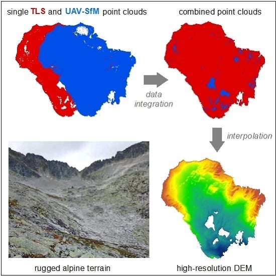
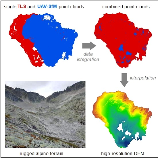
:Airborne and terrestrial laser scanning and close-range photogrammetry are frequently used for very high-resolution mapping of land surface. These techniques require a good strategy of mapping to provide full visibility of all areas otherwise the resulting data will contain areas with no data (data shadows). Especially, deglaciated rugged alpine terrain with abundant large boulders, vertical rock faces and polished roche-moutones surfaces complicated by poor accessibility for terrestrial mapping are still a challenge. In this paper, we present a novel methodological approach based on a combined use of terrestrial laser scanning (TLS) and close-range photogrammetry from an unmanned aerial vehicle (UAV) for generating a high-resolution point cloud and digital elevation model (DEM) of a complex alpine terrain. The approach is demonstrated using a small study area in the upper part of a deglaciated valley in the Tatry Mountains, Slovakia. The more accurate TLS point cloud was supplemented by the UAV point cloud in areas with insufficient TLS data coverage. The accuracy of the iterative closest point adjustment of the UAV and TLS point clouds was in the order of several centimeters but standard deviation of the mutual orientation of TLS scans was in the order of millimeters. The generated high-resolution DEM was compared to SRTM DEM, TanDEM-X and national DMR3 DEM products confirming an excellent applicability in a wide range of geomorphologic applications.
1. Introduction
Capturing terrain topography with a high spatial detail has become a common task in many research and engineering applications, which require sampling land surface heights (elevations) with spatial density and measurement precision in the order of millimeters to centimeters [1,2,3,4]. Currently, the most commonly used remote sensing methods for such a fine-scale 3D mapping comprise terrestrial laser scanning (TLS)—i.e., terrestrial lidar [5,6]—and close-range photogrammetry based on image matching by structure from motion, typically based on unmanned aerial vehicles as the sensor platforms (UAV-SfM) [7,8,9,10]. The main benefit of the technologies is in fast data acquisition and high accuracy—several millimeters for TLS [11,12,13] and several centimeters for UAV-SfM [14,15,16]. The achievable ultra-high spatial resolution provides means for analysing structural properties of rock outcrops [17,18], landslide dynamics [19], relative age of landforms [20], soil erosion [21], biomass [22], 3D city modelling [23] or archaeology [24]. Several studies [25,26,27,28] compared the accuracy of point clouds generated by TLS and UAV-SfM and/or digital elevation models (DEMs) derived from these sources of point clouds but without their integration into a single point cloud to generate a DEM.
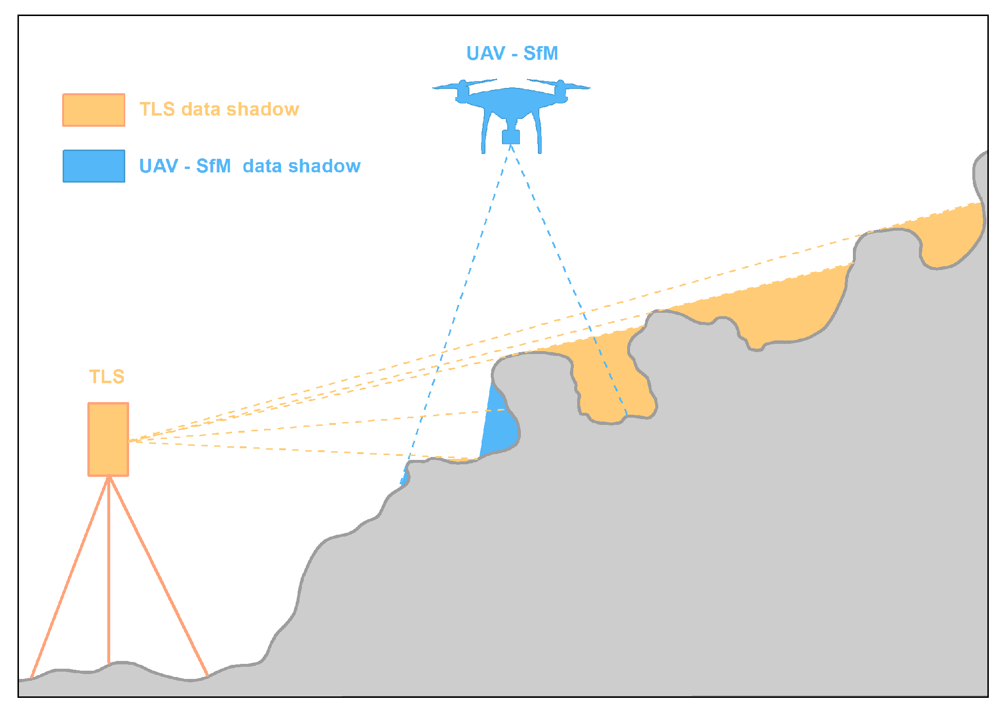
The general advantage of laser scanning over photogrammetry is in the ability of sampling several kinds of surfaces (e.g., top of vegetation canopy, inter-canopy surfaces, and ground) which are in the line of sight of the laser beam until impermeable surface restrains further penetration of the laser energy. UAV-SfM has become a low-cost alternative to TLS, generating point clouds with comparable accuracies to TLS albeit with the limitation of sampling the top surface in the field of view. Either way, in cases where TLS or UAV-SfM are used separately, data shadows originate in areas which are obscured in the sensor’s field of view [23,29] (Figure 1). Complementing the unsampled areas with the surface altitude measurements is possible by sensing the area from multiple positions and different viewing perspectives by changing the location of the sensor. Zhang and Lin [30] provide a systematic overview of the lidar and photogrammetric data fusion. Cawood et al. [7] showed there is no exclusive method for capturing complex 3D geometry in the case study of 3D modelling a large boulder with distinct geological structural features. Combination of TLS and UAV-SfM provided the most satisfying results to capture the geometric complexity of the object of interest for structural analysis. A similar approach of combining different viewing geometry of TLS and photogrammetry was demonstrated in 3D modelling of a historical city by [23]. Planning the data collection in the mentioned studies concerned environments with a relatively easy access for the technology and the surveying personnel.
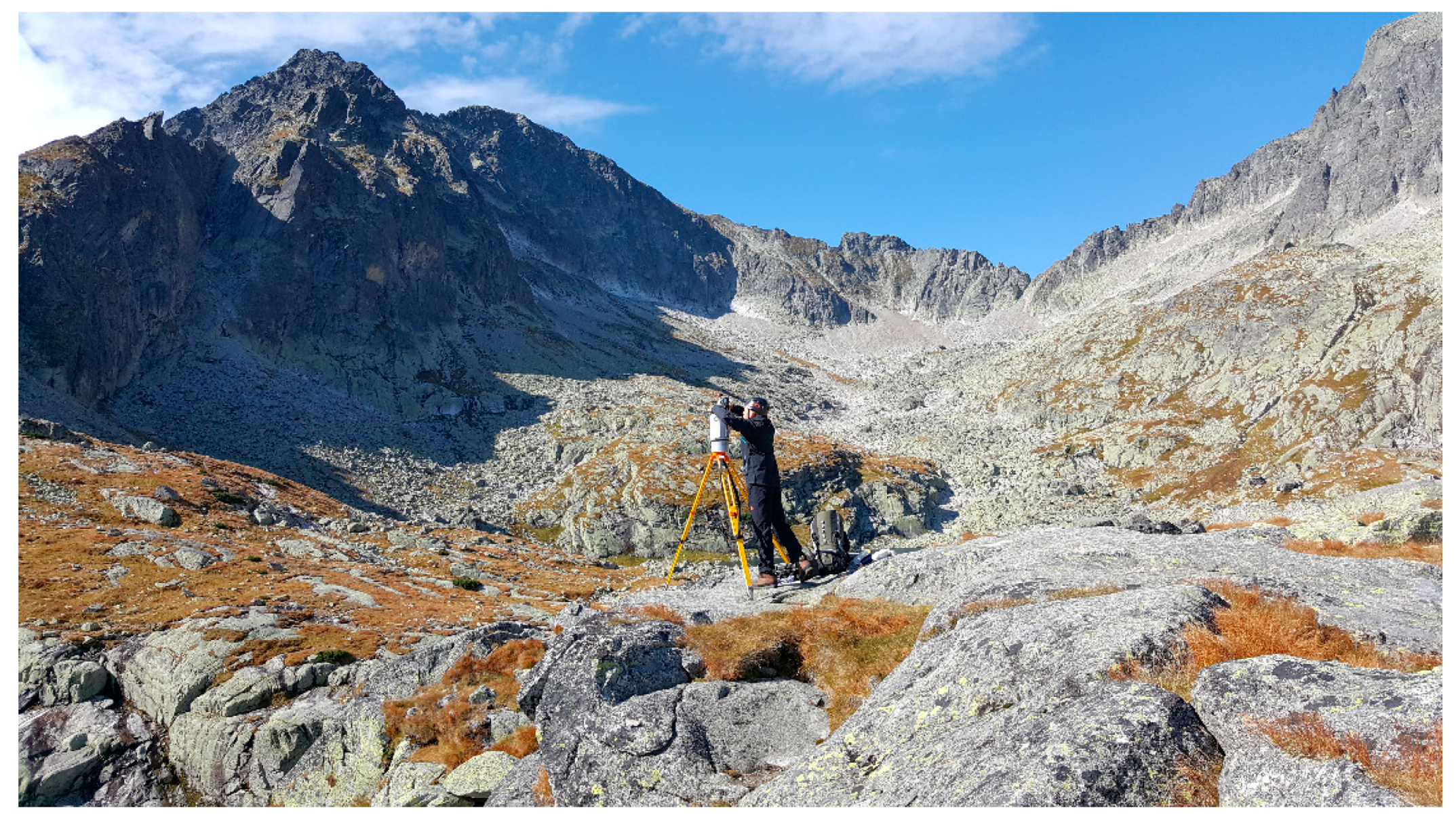
Deglaciated alpine landscape with landforms of different size, shape and verticality (Figure 2) pose a serious challenge for mapping with high sampling density and homogenous data coverage. Also, such areas are often inaccessible by convenient means of transportation such as a car or a helicopter and often access by foot is the sole option. Therefore, survey equipment has to be manually carried to reach the area of interest. In addition, the weather can change quickly, and the survey plan needs to be adapted accordingly. In many countries, alpine landscapes are protected areas of outstanding natural beauty with legal constraints for human activities and movement.
In many developed countries across the globe airborne lidar or photogrammetric data exist and the datasets are publicly available on a state-wide level. However, for pronounced rugged alpine areas, the spatial resolution and measurement accuracy of the existing digital elevation datasets can be still insufficient for specific tasks requiring very high accuracy and spatial resolutions. For example, Podgórski et al. [31] report that steep slopes in alpine areas introduce large errors in the TanDEM-X DEM dataset. For this reason, custom remote sensing data need to be acquired, mostly with UAV-SfM or TLS. Such high-resolution DEMs are often required for snow cover modelling [32,33], analysis of glacial morphogenesis [34], land surface dynamics [35,36] and associated land surface processes such as water flows and avalanches.
Several studies demonstrated the use of UAV-SfM for mapping rugged terrains such as alpine mountains [32], coastal cliffs [14], or volcanos [37]. However, these studies put the focus on validation of the UAV-SfM datasets and not on the integration of UAV-SfM with TLS point clouds. Iterative closest points (ICP) algorithm has become a popular method in mutual orientation of two spatially overlapping point clouds (i.e., point cloud registration). Combination of 3D point clouds from UAV-SfM and TLS with ICP was demonstrated for 3D building models and heritage sites [23,38,39]. The obvious advantage of this approach is a substantial reduction of data shadows and availability of photographic images for photorealistic visualisation. In these cases, the mapped scenes contained many objects with regular shapes allowing the achievement of a higher level of accuracy than in natural rugged alpine landscapes with much more complex morphology.
The alpine terrain exhibits many dynamic geomorphologic phenomena associated with mass movement such as landslides, erosion and rockfalls that frequently alter terrain surface morphology. Recording the effect of these processes requires a flexible mapping workflow which results in the digital elevation dataset having sufficient spatial detail and measurement accuracy for capturing the fine-scale morphology. In this paper, we hypothesise that the challenging task of 3D mapping the rugged alpine topography can be efficiently achieved with the combined use of TLS and UAV-SfM. We demonstrate this by our suggested workflow involving acquisition of 3D data by the two remote sensing techniques, data processing and combining the data into a final point cloud, DEM, and a 3D mesh surface. This approach is applied in a small study area comprising nested glacial cirques in the Tatry Mountains, the highest range of the Carpathians. The ultimate goal of the presented work is to generate a fine-scale 3D representation of the terrain surface applicable in geomorphological research of rugged alpine topography. The final 3D point cloud is made available for other studies via a 3D interactive web-interface as sharing and accessibility of the 3D spatial data is important to communicate the scientific outcomes. We also compare the generated DEM with other available DEM datasets for the mapped area. The presented workflow is transferable to other similar rugged environments to be used for high resolution geomorphological monitoring and mapping of small areas in the rugged alpine terrain.
2. Materials and Methods
2.1. Area of Interest
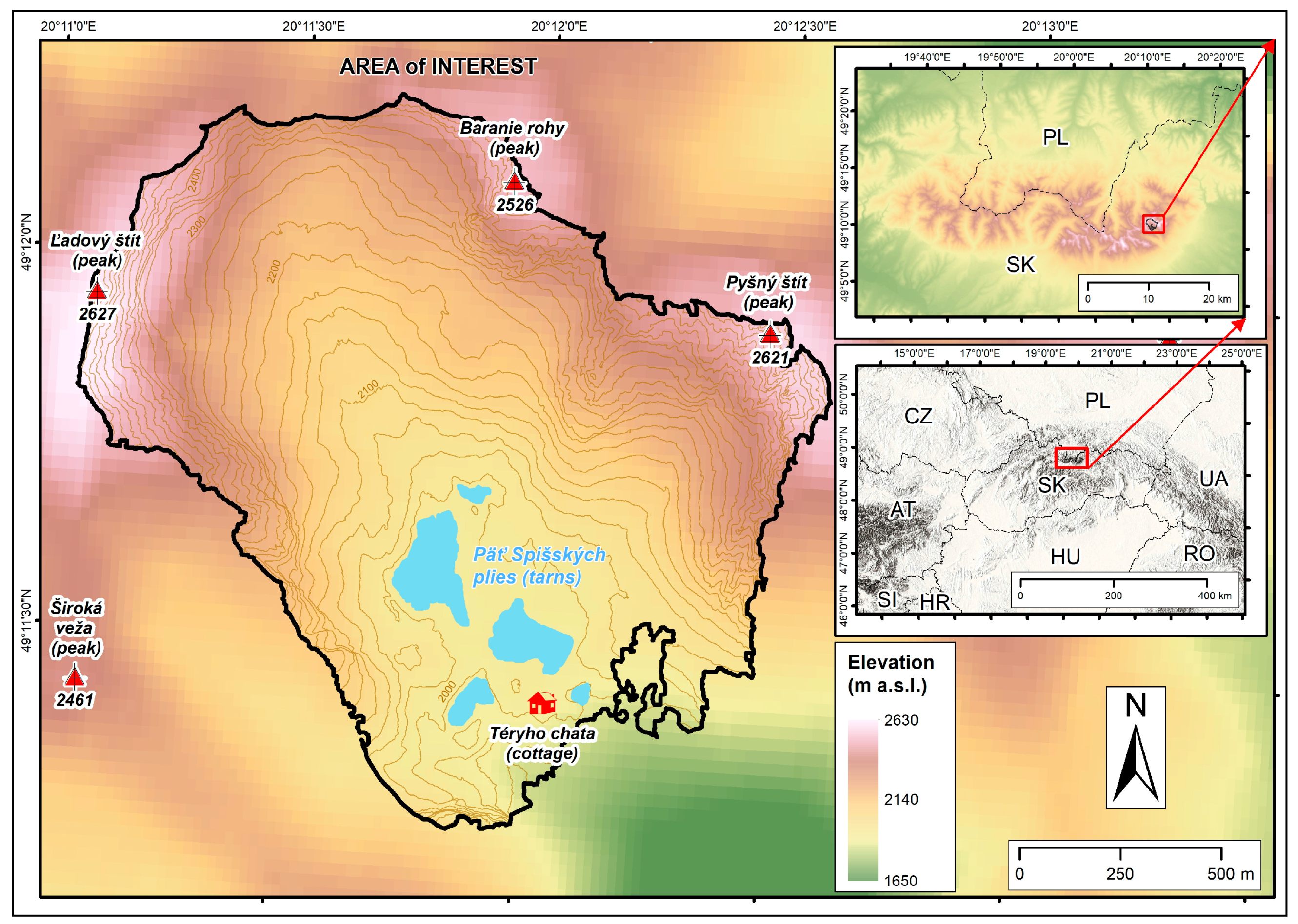
The area of interest is located in Vysoké Tatry (High Tatras)—the central part of the Tatry Mountains, where the Carpathians reach the highest elevation, displaying the most pronounced glacial morphology in the mountain range (Figure 2). The contemporary topography of High Tatras resulted from alpine glaciation altering with deglaciation stages in the Pleistocene while the massif has undergone a relatively rapid and continuous tectonic uplift since the Pliocene [40]. The glaciers carved ∼600–900-m-deep troughs and cirques with steep slopes separated by sharp ridges and peaks in altitudes from ∼2500 to 2655 m above sea level (m a.s.l.).
In particular, the area, which was subject to the remote sensing survey, comprises about 2 km2 of the upper part of the Malá Studená dolina valley (Figure 3). It is a glacial cirque incised into the southern part of the crystalline core consisting of biotite granodiorite-tonalite to muscovite-biotite granodiorite [41]. There are three compound cirques surrounded by headwalls up to 500 m high which form the upper part of the valley. The distinct glacial morphology of the area is modified by prominent gravity and cryogenic depositions forming extensive talus cones descending from the lower sections of the headwalls and ablation till and nivation ridges covering the central parts of the cirques floor. The bottoms of the cirques are situated at ∼2000 and 2190 m a.s.l., respectively. The depression parts of the cirques are filled with water forming five partially interconnected glacial lakes (tarns) from which the stream of Malý Studený potok flows out into the valley [42]. Rock steps up to 400 m high represent the transition from compound cirques down to the trough at the southeast edge of the area of interest.
Climate conditions of High Tatras are specific, determined by transition of ocean to continental climate which combines with the climate of high altitudes. The average annual temperature in the area of interest is −2.5 °C and temperatures not exceeding 0 °C occur approximately 160 days a year [43]. The average annual rainfall of 1870 mm per year is the highest in the region and most precipitation falls in the form of snow. The snow cover remains in the area for approximately 180 days a year [43]. Such a climate allows only for a limited grass cover with rare clusters of mountain pine; therefore, the majority of the terrain is exposed bedrock or scree.
Almost the entire extent of the Tatry Mountains is protected by law as a national park (TANAP) with the highest level of natural protection in Slovakia [44]. Moreover, the surveyed area is a part of specially protected natural reserve of Studené doliny for being a refuge of various plant and zoological species and for outstanding natural beauty. Therefore, human activities are limited and road access by car is restricted to lower parts of the mountains up to about 1500 m a.s.l. with tourist resorts. Upper parts are accessible only by foot via trails or elsewhere with mountaineering equipment and special permission. The mountain cottage of Téryho chata is situated in the south of the area of interest providing accommodation and refuge in case of bad weather or mountain rescue throughout the year. For this reason, a number of human activities such as supplying mountain cottages, treatment and transporting wounded by rescuers have been hampered.
2.2. Data Collection
The study area was mapped in two separate mapping campaigns in September and October 2017. Four persons were involved in carrying the necessary instruments and performing the field work. The weight of surveying equipment and accessories was about 50 kg in total and had to be hand-delivered walking for about 3 h using the existing tourist trail. The equipment comprised two dual-frequency GNSS receivers Topcon Hyper II, a Riegl VZ-1000 long range laser scanner with an integrated Nikon D-700 camera, an UAV quadcopter DJI Phantom 4 with an integrated 12-megapixel FC330 camera (focal length 3.61 mm) mounted on 3-axes gimbal.
Careful planning preceded the work in the mountains. We analysed available orthoimagery on Google Earth, and national DEM (DMR3) was used to do a preliminary assessment of the visibility for optimal placement of the laser scanner and for determining optimal paths for transport between the intended scanner positions. Once in the field, the preliminary plan had to be modified in some cases for safety of transportation between scanner positions. The laser scanner was preferably placed on stable, exposed bedrock or large boulders avoiding scree debris surface so that the device remained stable during scanning and the scanner field of view was as wide as possible. In addition, the terrestrial laser scanner was tested, especially its range, scanning duration at various settings and transport options in rugged terrain. The maximum recorded range of the scanner was 1500 m and the dispersion of point measurements at such a distance was approximately 0.6 m. The planning also involved consideration of the weather. We aimed for clear sky, calm wind and no snow conditions to perform the work in a single campaign. First, the site was surveyed during 13 and 14 September 2017 when the snow cover was at minimum that year. The sky was clear; the maximum air temperature was about 15 °C. The wind speed was 8–12 m/s which was at the upper limit for flying the UAV. The land surface was dry which was favourable for TLS. The field work began at 13:00 setting up a GNSS base station near the cottage of Téryho chata. Position of the base station was located by real-time kinematic (RTK) GNSS positioning with a mobile broadband connection to the network of the Slovak real-time positioning service (SKPOS) within the national S-JTSK03 coordinate system (EPSG code: 5514) with vertical datum Baltic after adjustment (Bpv). The overall accuracy of the RTK GNSS positioning ranged between 1–2 cm (1σ). The baseline to the closest SKPOS base station in Gánovce was 20 km southeast. Meanwhile, the TLS and UAV-SfM surveys had begun.
The RTK GNSS positioning was used to locate 104 ground control points (GCPs) on the terrain, free bedrock or large boulders. There were 4 black and white checker board markers (20 cm by 20 cm) distributed at a distance of 5–10 m around 4 scan positions and their central point was measured with the RTK GNSS. By this means, 16 tie points originated for transforming the TLS data into the national coordinate system. In addition, there were 21 GCPs collected during the campaign in September 2017 between the TLS positions (Figure 4). The rapidly varying weather conditions, especially, increasing wind speed, induced another campaign one month later to supplement the data voids with new measurements. Therefore, another survey campaign was performed on 19 October 2017. The mapping involved TLS and UAV-SfM without positioning any GCPs with GNSS. Additional 67 GCPs were collected with RTK GNSS in July 2018 to supplement the GCPs dataset with validation points (Figure 4).
2.3. Terrestrial Laser Scanning
Data collection with TLS in the September campaign began with a position near the cottage of Téryho chata in the south and continued to the northwest up toward the valley head. Selection of the consecutive position of the scanner considered terrain ruggedness and accessibility so that possible data shadows are eliminated and sufficient spatial overlap of point clouds from two adjacent positions is ensured. Therefore, the separation of positions was not regular (Figure 4); the scanner was preferably located on sites where it was possible to efficiently map larger parts of the area of interest. To ensure an optimal coverage of the area by point measurements, different settings of the scanner were used for laser scanning. Given the spatial extent of the area of interest, scanning from 6 positions with a 70 kHz pulse repetition rate (PRR) and scanning range of more than 1400 m was performed. For some positions, scanning with 300 kHz PRR and a range of 450 m or with 150 kHz PRR and a range of 950 m were used to densify data at overlap positions. In total, TLS was performed from 15 positions during the first campaign in September 2017 which were supplemented by 7 scan positions in October 2017 (Figure 4). The scanning positions were distributed in the south, west and north of the area of interest which was limited by the accessibility and safe transport of the equipment. Figure 5 maps the data coverage from each scanning position for both dates of the TLS survey where data voids can be seen as white areas. The reasons of data shadows are to do with terrain occlusion or poor reflection of the laser light from the surface of water or snow.
Raw TLS data was processed in the RiSCAN PRO software. First, the individual point clouds (scans) acquired from each scanning position were assigned RGB values representing natural colour from the photographs taken with the camera integrated on the scanner. The information on colour helped in interpretation of the points and in finding and co-locating the objects of interest in the following procedure of mutual orientation of the scans (registration). The registration was performed between two or more overlapping point clouds based on identical points. This procedure consisted of two steps: manual and automatic registration. The Riegl VZ-1000 terrestrial laser scanner comprises an integrated GPS receiver that measures geographic coordinates of the scanner position with accuracy of several decimeters to meters. The in-built magnetic compass provides measurement of the azimuth towards magnetic north. Measurements of the two devices are used for coarse placing of the individual scans in a global (common) coordinate system and coarse orientation of the scans. This feature facilitates and speeds up finding identical points of the spatially overlapping TLS point clouds in the following step of the coarse registration. The procedure requires at least 4 identical points to be identified between two overlapping scans. This principle also works with automatic registration that is implemented as the Multi Station Adjustment (MSA) in RiSCAN PRO. Based on the selected parameters, the MSA generates polydata. These are the points identified as identical in the areas of overlap for two or more scans being mutually registered. The MSA method uses the iterative closest points (ICP) algorithm which minimises the 3D distance between the polydata points by translating and/or rotating the entire point cloud along X, Y, and Z axes until the least possible distance between the polydata points is reached [39,45,46] (Figure 6). The TLS point clouds (scans) were registered in such a way that the position and orientation of the first scan were locked and the second scan was translated and rotated until the smallest standard deviation was reached with respect to the polydata of first scan. After registration, the position and orientation of the first and second scan was locked and the position and orientation of the third scan was adjusted by the MSA. The procedure continued in this way until all scans were registered as precisely as possible in a common coordinate system. Finally, the position and orientation of all scans was unlocked apart from the central scan which remained locked, and the MSA was performed again to redistribute the adjustment error more evenly within the point cloud.
For georeferencing the final TLS point cloud, central points of the 16 black and white checker board targets placed within the scanned scenes were manually identified and they were assigned with the coordinates measured by the RTK GNSS method. By this means, the final TLS point cloud was transformed from the global coordinate system (Cartesian WGS84) into the national projection coordinate system (EPSG: 5514) with the Bpv vertical datum.
For the data voids still present in the TLS point cloud another campaign was performed on 19 October 2017. The mapping involved TLS and UAV-SfM methods. The TLS was performed in the northern part of the valley from 7 scan positions to increase the point density in this area. The MSA method in the RiSCAN PRO software was used to mutually register the acquired TLS point clouds as was described earlier. The resulting October TLS point cloud was oriented with respect to the September TLS point cloud and thus georeferenced in the national coordinate system. A unified TLS point cloud originated.
As the last step, the final TLS point cloud was cleaned by manually removing the noise points (e.g., reflections from water table or dust particles in the air) and the points representing the building of the Téryho chata cottage. The area under the building was kept unsampled but the terrain under the building was approximated by the interpolation function in the production of the final DEM. In the area of interest, there is virtually no vegetation cover which could effectively occlude the terrain surface for the emitted laser light. Point returns from occasional patches of low grass, moss or individual dwarf pine trees present in the lower parts of the area were inspected. We decided that applying vegetation filter is not required to remove the non-ground returns as the height difference between top parts of the grass or dwarf pines and the ground was below 0.2 m.
2.4. UAV Digital Photogrammetry
The UAV-SfM method provides a different, vertical to subvertical, viewing angle which increases the capability of mapping in areas of pronounced vertical relief obscured for TLS where data shadows originated (Figure 1). The UAV-SfM method also supplements the point data with orthoimagery. We decided to fly the UAV in the manual mode despite the fact that the system is capable of flying according to a pre-set trajectory and camera settings. The main reason was the safety of flight, i.e., to have a direct control over the UAV during the flight in case of wind gusts and uncertain visibility of GPS satellites in such a pronounced vertical relief of the mapped area (over 600 m). There were two 20-min flights performed in September 2017, taking 352 images in total covering the entire area of interest and its surroundings with an average spatial resolution of 17 cm. The average flying height relative to the take-off position near the cottage of Téryho chata was 464 m. The range between the UAV and the terrain was at least 100 m. In October 2017, the UAV was manually flown at a lower average flight height of 258 m taking 618 images with average spatial resolution of 9.5 cm covering 80% of the area of interest. The acquired imagery was processed in the Agisoft PhotoScan software resulting in 3D point clouds and orthoimagery. Almost 13 million and 90 million points were extracted from the September and October image collections, respectively. The data were georeferenced in the WGS84 geographic coordinate system (EPSG: 4326) based on the positioning data recorded by the on-board GPS antenna for the image exposures. More details on the settings and output statistics of the data processing are found in the reports provided as Supplementary files (UAV reports S2).
2.5. TLS and UAV-SfM Data Fusion
Both independently acquired datasets locally contained data shadows (voids) or sparse coverage which could be reduced by fusing the TLS and UAV-SfM point clouds. The assumption in this procedure was that the TLS data are internally registered (mutually oriented) with a higher level of accuracy than the UAV-SfM points. While the TLS point cloud was georeferenced using GCPs, there were no GCPs acquired for such georeferencing of the UAV-SfM data. The reasons were practical as placing the GCPs targets in the area of interest and measuring their location with GNSS would have to be done before flying the UAV. This case would require additional manpower or more time which was not feasible in such a rugged terrain. Mapping by UAVs is strongly influenced by weather conditions since flying in strong wind and rain is very problematic and also dangerous. Fog or low altitude cloudiness decrease the visibility of land surface. In High Tatras and other similar alpine areas, the weather can change very quickly. Therefore, it was preferred to perform the UAV-SfM data collection as soon as possible and the generated point clouds were georeferenced in the national coordinate system by registering them on the already georeferenced final TLS point cloud with the MSA method in the RiSCAN PRO software.
First, coarse registration based on 4 manually identified points was performed to place the UAV-SfM and TLS point clouds closer together in the 3D space reaching standard deviation of mutual displacement between the two point clouds of 0.5 m. Afterwards, the application of the MSA automatic registration method followed. The MSA method identified only several tens of identical points (i.e., polydata) between the TLS and UAV-SfM point clouds in areas of markedly differing point densities. The automatic registration process was performed in several steps, with each step further reducing the values of the search window parameters and the point cloud rotation angle [39,45,46]. By decreasing the values of these parameters, the registration error was reduced from decimeters to several centimeters. The UAV-SfM dataset contained less morphological detail than the TLS point dataset as the point density was much lower in the UAV-SfM data. Hence, further reduction of the standard deviation of mutual adjustment reached the limits at several centimeters. For this reason, the UAV-SfM points were used for the fusion with the final TLS point cloud only in the areas larger than 2 m2 where no spatial coverage of the TLS points existed. In this way, the elevation points covered the areas of TLS data shadows. There was no vegetation present in such places.
The point cloud resulting from the TLS and UAV-SfM fusion was decimated with a 0.5 m spacing of 3D distance in the Cloud Compare software to homogenise the diverse spatial density of points and to reduce data redundancy for the DEM generation procedure. The final point cloud thus contained 4 points/m2. The colour information was kept with the pre-decimated TLS data, but it was removed from the decimated TLS point cloud as it provided mixed colours from two different TLS campaigns. After the point cloud fusion, the points were assigned with the RGB colour from the orthoimagery, which provided consistent colour information across the area with higher resolution (0.17 cm) than the final point cloud had (0.5 m).
2.6. Generating a Digital Elevation Model
The point cloud is a discontinuous digital representation of the mapped land surface, which is not directly applicable for modelling phenomena and processes in the landscape. Typically, point clouds are used as input data for generating continuous raster-based DEMs. We considered the final point cloud as the representation of terrain surface (ground) as there was limited number of above-ground features present in the area of interest and the point cloud was subject to filtering (Section 2.3 and Section 2.5). Therefore, we will further use the term DEM to refer to a digital terrain model instead of digital surface model (DSM). In our case, we preferred spatial interpolation procedure generating smooth continuous DEM surface instead of direct conversion of point elevations to raster grid. The method used is implemented as the parallelised v.surf.rst module in the open-source GRASS GIS 7.6.1 software [47,48]. The module uses regularised spline with tension and smoothing [49,50] for interpolating the input height values into centres of a raster grid. The used interpolation tool allows for fine tuning the spline interpolation function via a set of parameters controlling the stiffness and exactness (smoothness) of the resulting surface. The default parameters were changed in the case of the tension parameter to 20, the smoothing parameter to 0.8 and the minimum distance between points to 0.4 m. The final DEM was interpolated in a squared grid of 0.5 m grid cell-size which corresponded to the density of the final, spatially homogenised (i.e., decimated) point cloud.
The DEM data structure reaches limitations in modelling pronounced verticality of land surface, which often occurs in rugged alpine terrain or in caves [51]. Therefore, we also generated a 3D vector-based surface model (i.e., polyhedral mesh) using the Poisson reconstruction [52] implemented in the Cloud Compare software.
2.7. Comparison with Other Freely Available DEM Datasets
The extreme morphology of the area of interest has been captured by other publicly available DEM data sources. To support the relevance of the performed research, we selected three datasets and calculated vertical differences with respect to the final DEM derived from the fused TLS and UAV-SfM data. The following DEM products were used: SRTM (SRTMGL1-V003) DEM, TanDEM-X, and the national DMR3 DEM. The SRTM dataset [53] was acquired with 1 arc-second spatial resolution on global scale in 2000 by synthetic aperture radar (SAR) interferometry during a single shuttle radar topographic mission. Further details on data SRTM data acquisition are reported in [54]. The SRTM data have been widely used for land surface analysis across various disciplines and they were validated for different kinds of topographies [55]. The spatial resolution in the area of interest is about 27 m for the SRTM data used. Additionally, the overall vertical error in the final product is below 9 m [55].
The TanDEM-X data were acquired by radar interferometry with a constellation of two satellites between 2010–2014 with repeated data acquisition (at least twice up to four passes) [56]. The DEM product was made available since September 2016. This DEM product is a new generation global DEM providing resolution of 0.4 arc second which can be seen as one of the most consistent, highly accurate and completest global DEM data sets of the Earth surface. Global assessment summarised by [57,58,59] reports overall vertical accuracy below 2 m which is subject to land cover and surface slope angle on local scale.
The third DEM dataset involved in the comparison was the national DMR3 DEM derived from vectorised contours from topographic maps at 1:10,000 and 1:25,000 scale and interpolated into a grid of 10 m by 10 m cell-size. The dataset was provided by the Geodetic and Cartographic Institute of the Slovak Republic.
The final TLS-UAV-SfM DEM was resampled to match the original resolution of each of the three compared DEMs: 30 m for SRTM, 12 m for TanDEM-X and 10 m cell size for DMR3, respectively. The elevations were unified into a common WGS84 geodetic datum with ellipsoidal heights. Afterwards, the resampled final DEM was subtracted from the compared DEM in a map algebra operation using the r.mapcalc module and the statistics of the elevation residuals were calculated with the r.univar module in GRASS GIS, respectively.
3. Results
The complete methodology for mapping rugged alpine terrain using a combined use of TLS and UAV-SfM photogrammetry is schematically presented in the following flowchart (Figure 7). The workflow contains four major steps: data acquisition, data processing, point cloud integration and generation of a land surface model in the form of a DEM and 3D mesh. The data acquisition involved terrestrial laser scanning with a Riegl VZ-1000 and UAV photogrammetry with a DJI Phantom 4 quadrocopter with an integrated Ultra HD camera. The two methods provide different view aspects of the mapped area which enabled acquiring more complete and homogenous coverage of data in such a complex topography. Additionally, RTK GNSS with a base and a rover constellation was used to acquire GCPs for georeferencing the TLS data and for validation purposes. The data processing consisted of: (i) mutual registration of point clouds generated from different TLS scanning positions; (ii) TLS point cloud georeferencing in national coordinate system; (iii) generating orthoimagery and UAV-SfM point cloud; and (iv) extracting points from UAV-SfM point cloud in data shadows of the TLS point cloud and merging the extracted points with the TLS dataset. The presented approach enabled digital reconstruction of a rugged and hard to access alpine terrain in a small area in the Tatry Mountains in Slovakia. The following subsections present the resulting datasets and evaluate their height accuracy and applicability in geomorphologic research in comparison to other freely available DEM products.
3.1. Generated Point Clouds
Mapping with TLS and UAV-SfM generated dense point clouds capturing the 3D geometry of the explored area as a vector data representation. All the data acquired in the Malá Studená dolina valley were cropped by the polygon of the area of interest covering about 2 km2 (Figure 3 and Figure 4).
TLS generated over 264 million points from 22 scan positions. The standard deviation of consecutive registration of individual scans ranged from 2.6 mm to 12.9 mm, with an average standard deviation of 6.1 mm. After registration of all of the scans, the central scan position was selected (no. 7) whose position and orientation were kept locked and all other scanning positions were once again registered with respect to it reaching the standard deviation of registration of 4.2 mm. By registering all of the scans, a single point cloud was created representing the terrain in the area of interest. The resulting TLS clouds were georeferenced with 16 GCPs reaching the standard deviation of coordinate transformation of 33.2 mm.
The TLS point cloud density was markedly heterogeneous (Figure 8), generally decreasing with the increasing distance from the scanner position. Therefore, there were almost 100,000 points/m2 in places near the scanner and only 1 point/m2 at the largest range. The average density of TLS points in the area of interest was approximately 130 points/m2. With TLS or UAV-SfM applied in such non-vegetated area, the points density refers to the points on terrain or boulders. Vast majority of recorded points were first echoes returned from the rock blocks or exposed bedrock. This is important to note as [60] it emphasises the importance of referring to the type of returns not just the overall number of points per unit area.
Nevertheless, the areas without any points were still present. To complement such places with 3D point measurements, UAV-SfM was deployed. The method also produced orthoimagery and a 3D point cloud yet from a vertical viewing angle different to the TLS method. As shown in Table 1, over 12 million points were extracted from the imagery in September. There were over 89 million points generated from the October UAV data. This difference is caused by lowering the above ground flight altitude in October which resulted in finer ground sampling distance (GSD). Average point density therefore ranged from 4 points/m2 (September) to 47 points/m2 (October) (Figure 9).
The final UAV 3D point clouds were internally consistent but they were only coarsely georeferenced with the WGS84 coordinates (EPSG: 4326) measured by the internal GPS antenna of the UAV and recorded in the EXIF information of the images. No GCPs were used for the purpose of georeferencing to save time and manpower. Instead, the UAV-SfM clouds from September and from October were georeferenced by spatially registering them to the final TLS point cloud using the MSA method (Section 2.3, Section 2.5). Standard deviation of UAV-SfM data registration was 0.11 m and 0.13 m, for September and October respectively. Even though the UAV-SfM data for September had a lower spatial density than the October dataset, the daylight conditions during data collection were better than in October. As a result, the September data had higher horizontal and especially vertical accuracy than the October dataset. Consequently, the integration of TLS and UAV-SfM data in September only was preferred as a lower standard deviation was reached than with the integration of October data.
The absolute accuracy of the final point cloud was assessed as a cloud-to-cloud distance between 104 independent GCPs measured with RTK GNSS and the georeferenced TLS point cloud (Table 1). The resulting mean 3D distance was 0.114 m and the root mean square distance was 0.143 m.
3.2. Final DEM and Comparison with Other DEM Data Sources
DEMs created from individual TLS or UAV-SfM point clouds would not be sufficiently accurate due to data shadows and low point density in some areas. However, the integrated TLS and UAV-SfM data (September) homogeneously cover the whole area of interest. The final DEM derived from the combined TLS and UAV-SfM data is shown in Figure 10.
The quality of the final DEM was evaluated by assessing its vertical accuracy and visual inspection and comparison to the existing DEMs for the area of interest. The DEM accuracy assessment is reported in Table 1. The same GCPs were used in calculating the elevation differences as in the case of validating the georeferencing accuracy of the final point cloud. The mean vertical residual value reached −0.461 m suggesting systematic underestimation of elevation by the final DEM. The reported percentiles also reveal the negative bias. The root mean squared difference (RMSE) value of 0.574 m indicates overall fit to the reference points. The value is higher than for the point cloud RMSE (0.143 m) as the interpolation of the DEM involved surface smoothing and the number of input points was reduced in comparison with the input point cloud (i.e., controlled by the dmin parameter of 0.4 m). Thus, the resulting DEM with 0.5 m grid cell size smoothed the rough topography with elevations varying across shorter distances. The DEM cell is assigned just one altitude, but this space covers a part of the large boulders and gaps between them. For safety reasons, the GCPs were selected on stable parts of the terrain, such as top parts of large boulders, or exposed bedrock which were likely to be captured by the TLS or UAV-SfM methods. This opens a question: What is the actual terrain surface in such a landscape? Does it comprise boulders or the surface of bedrock underneath them? Therefore, collection of GCPs should a priori consider the spatial resolution of DEM and scale-dependence of the sampled surface.
The validation of the point cloud suggests the overall match of the input dataset with the reference GCPs is high and more than acceptable for the geomorphological research. The relative decrease of the final DEM vertical accuracy is also acceptable, and the accuracy could be improved by increasing the spatial resolution of the DEM which was not desired for the purposes of future research. A more detailed and accurate DEM can be generated from the input point cloud if needed.
Nevertheless, the final DEM resulting from the data fusion represents the most detailed 3D representation of rugged alpine terrain of the highest part of the Tatry Mountains (Figure 10). To date, available DEMs for Slovakia were produced predominantly from vectorised contours digitised from topographic maps. The DMR3 DEM product with 10-m spatial resolution is the most detailed DEM data source to date. However, topographic maps often do not contain complete elevation information in rugged rocky areas. These areas are usually represented only by cartographic symbols with no contours. For this reason, the DMR3 is not sufficiently accurate in these areas, especially on very steep slopes. A visual comparison of available DEMs are presented in Figure 11. The SRTM DEM (Figure 11A) is too smooth with many geomorphologic features missing. The TanDEM-X DEM (Figure 11B) is very noisy on steep slopes; however, flatter areas contain many desired spatial details of land surface. The national DMR3 DEM (Figure 11C) is also too smooth, with missing smaller geomorphologic features.
SRTM, TanDEM-X and DMR3 DEMs were compared in terms of vertical difference against the derived TLS-UV-SfM dataset. The results are summarised in Table 2 and in Figure 12. The calculated summary statistics for vertical differences in the digital surfaces indicate how closely the existing DEM datasets approximate the reference DEM generated from the TLS-UAV-SfM data. Digital surface of differences (DOD) represent vertical differences between the evaluated DEM and the resampled reference DEM so that both surfaces have corresponding spatial resolutions and become comparable. The negative mean difference indicates that all three evaluated DEMs systematically underestimate the elevations in the area of interest. This effect is the most pronounced in the TanDEM-X data which is also supported by the highest standard deviation and root mean squared difference (RMSE). However, the more robust measures such as median, the 1st and the 3rd quartile and their range show that the dispersion of the lower half of the vertical differences is larger for the SRTM data. The spatial pattern of DODs in Figure 12A,B reveals that the differences of SRTM vary smoothly while the DOD of TanDEM-X shows a large central area of values between −5 to +5 m suggesting a good correspondence with the reference DEM. Larger systematic bias can be attributed to the coarser spatial resolution of SRTM which causes smoothing of elevations in this extreme topography. The extreme differences concentrate along the edges of the study area where the vertical relief and slope angle are also extreme (Figure 12A). This fact is the most pronounced with the TanDEM-X data in Figure 12B. Large negative differences cluster near extremely steep which likely relates to the existence of radar signal shadows during data collection. The same applies to the SRTM data even though the extreme differences are much lower. These results confirm the findings of Podgórski et al. [31] on poor performance of TanDEM-X data on very steep slopes. The rest of the area shows a close vertical correspondence with the reference data. The DMR3 DEM reported the lowest differences in the order of few meters which is in accordance with the data specifications by the provider. Larger differences of several tens of meters occur on extreme topographies within the area (Figure 12C). Vertical profiles of all four DEMs in Figure 12D demonstrate the findings described according to the calculated statistics.
3.3. Applications of DEM and 3D Point Cloud
The final DEM represents land surface of various morphometry (Figure 10). On one hand, there are planar forms such as steep cliffs, smooth rôches moutonnées and glacially polished surfaces. On the other hand, scree slopes, plucked surfaces or moraines form rugged land surface. These forms are not quantitatively depicted in contemporary maps or digital elevation datasets available for this area of the Tatry Mountains. Airborne lidar was successfully deployed in Poland for state-wide mapping. The point density in the Polish part of Tatry reaches 4 points/m2 with vertical accuracy of 15 cm [61]. In Slovakia, airborne lidar has not been deployed on the state-level to date. Contours of topographic maps have been the main data source traditionally used for generating DEMs of Tatry in Slovakia, but they are replaced with symbols of steep and rocky surface for this kind of areas. The maps originated from photogrammetric measurements using aerial imagery which, however, was hampered by shadows in such a markedly vertically dissected landscape. The associated vertical and horizontal error in the order of few meters did not allow for ascertaining the absolute and relative elevations with sufficient accuracy for the purposes of detailed study of the recent processes and valley development. Using the DEM product derived in this study we exactly identified relatively flat areas and assigned them with elevation (Figure 13), which provides quantitative indicators of the development of stepped glacial cirque.
Recent developments in web-based 3D technologies have enabled interactive visualisation and analysis of large 3D point clouds which in turn enhances communication of the scientific results to wider audience [62]. These reasons motivated us to generate a stand-alone LiDAR Web portal enabling other researchers, professionals or public to explore the dataset without any need for special skills in computer graphics, geographic information science, installation of a special software or any additional plugins. Only a standard web browser and internet connection are required. The web portal was generated using the laspublish software utility of the LAStools package [63] which uses the Potree open-source WebGL based renderer [64,65,66]. Potree is capable of efficiently visualizing nearly 600 billion points in real-time via the Internet, changing colouring of points, performing measurement of 2D and 3D length, 3D area, volumes, generating vertical profiles, and exporting data. Figure 14 demonstrates these capabilities and the presented dataset can be accessed via the link: https://geografia.science.upjs.sk/webshared/Laspublish/Tatry/Tatry.html.
4. Discussion
The presented approach of combined use of TLS and UAV-SfM data in mapping rugged alpine terrain has several advantages. It provides a valuable flexibility in periodic mapping of small alpine areas, which is not economically and practically feasible by standard airborne laser scanning and photogrammetric methods. It provides more homogeneous spatially distributed point clouds which is important for creation of a DEM with spatially consistent quality using spatial interpolation. It should be emphasised that the generated dense point clouds are valuable and unique for the area in terms of geometric accuracy and the captured level of detail. To date, national elevation datasets of such alpine areas in Slovakia were acquired by aerial photogrammetry and vectorised topographic contours with spatial resolution of several meters. Other data available for the region comprise even coarser datasets such as the TanDEM-X DEM and the SRTM DEM derived by interferometric radar with a global coverage. These datasets are smoothed in some places or they contain noise in comparison with the final DEM resampled to the equivalent resolutions. This outcome hampers the applicability of the SRTM and TanDEM-X data in very detailed geomorphological research of the study area. Similar accuracy issues were observed in other areas with extremely rugged terrain [31,67].
Coarse DEMs are insufficient for analysing the rugged alpine morphology and for abundant presence of loose sediments of different sizes ranging from small scree to large boulders. Especially, it holds for detailed analysis and modelling of shallow recent land surface processes, such as runoff, bioturbation or solifluction which operate on a finer spatial scale than the coarse DEMs represent. Conversely, the high-resolution DEM created by the TLS and UAV-SfM data fusion can be used to identify and analyse a wide range of specific landforms and geomorphologic processes. It opens new possibilities for multiscale geomorphic modelling and segmentation leading to reveal a comprehensive nested hierarchy of landforms and land surface processes [68]. Indeed, a generalised (i.e., spatially coarser) DEM can suit the analysis of massive landforms and processes. However, using such a less detailed DEM is not the appropriate solution since the DEM is generalised in a random (i.e., erroneous or uncontrolled) fashion which causes the altitude and derived values of geomorphometric parameters to be distorted or biased. On the other hand, a high resolution and accurate DEM can be generalised in a controlled fashion providing a better solution for geomorphological research across multiple scales.
The orthophoto images can be used for photorealistic 3D visualization such as for 3D city models. The 3D point data could be used for modelling and planning search and rescue operations since the area is popular among tourists and mountaineers. The generated web-based tool enhances communication of the results. It is a user-friendly environment providing means for non-specialists to draw cross-sections, and conduct various types of 3D measurement, changing the displayed characteristics or extracting the 3D points for custom purposes (e.g., 3D printing).
The proposed approach also has limitations. It requires extensive field work with several hours of surveying depending on the extent of the area with limited accessibility by a car or other means for convenient transport of the required equipment. A long-range laser scanner, such as Riegl VZ-1000, has a clear advantage and saves a lot of time during surveying. However, its approximate weight of 12 kg complicates transport of the scanner and selection of optimal scanning position, especially in areas accessible only by foot and with considerable difficulties. Therefore, safer positions were preferred compromising the field of view.
The combined use of TLS and UAV-SfM was feasible as there is very limited vegetation cover in the area of interest, comprising occasional patches of grass and dwarf pine in the lower parts. Both methods generate most favourable representation of terrain unless dense vegetation, boulders, or buildings occlude the terrain surface. While TLS can penetrate vegetation cover into some extent, slant viewing angles from terrestrial platform, such as tripod, restrain the laser from reaching the ground through grass, dwarf coniferous trees. Reaching a uniform or homogenous point coverage with TLS is strongly limited by the number of scanning positions, their constellation, and mutual distance. The point density decreases with increasing range from the scanner. Large boulders of glacial moraines are abundant with TLS data shadows. In such cases, the vertical perspective of UAV-SfM helps to sample data but vegetation still occludes the ground. Shadows cast by the boulders or steep walls deteriorate the capability of the SfM method to find corresponding points in the shadowed parts where, on the other hand, TLS is applicable since it is an active remote sensing method. It is important to target the point density to the purpose of the resulting data. In our case, 0.5 m minimal spacing across the area was considered sufficient to represent the terrain topography.
Also, the surveying by UAVs or TLS depends on favourable meteorological conditions which can quickly turn into harsh weather in the mountains. In turn, the weather affects accuracy of surveying. Therefore, the use of these mapping methods requires careful planning and quick realization. Time of day and seasonality are other factors which can affect especially the quality of UAV-SfM data for differing light conditions. UAV mapping in October generated more points than in September, suggesting that October data captured the landscape with a higher level of detail. However, with regard to horizontal and, in particular, vertical accuracy, the data obtained in September could be more accurate. Ideally, capturing the imagery should be performed about noon with sky covered by clouds which disperse the sun light evenly. Meeting such requirements becomes often not feasible in planning the survey in a remote and hardly accessible area. In our case, the shadows cast by the pronounced terrain features were longer in the morning of the October campaign covering larger areas than during the flight about noon of the September campaign. In October, the sun is considerably lower above the horizon than in September which in combination with the NW–SE orientation of the valley made the terrain illuminated unevenly. Such an uneven illumination of the terrain caused lower vertical and horizontal accuracy of the October point cloud overall.
The limitation of a DEM in representing the alpine topography manifests in areas of extremely steep rock walls or overhangs. This is because a single DEM cell can represent only a single land surface elevation value. Although 3D point data were recorded for such forms, they are averaged in the DEM interpolation procedure resulting in a single elevation value per cell. The solution for analysing geomorphometric properties of such specific landforms is in modelling the surface as a 3D mesh. Figure 15 compares the derived elevation gradient (i.e., slope angle) for the DEM surface (Figure 15A) and 3D mesh surface (Figure 15B). One drawback of such a 3D data structure is that it has to be created and analysed in a specialised 3D software (e.g., Cloud Compare, Meshlab, Geomagic Wrap) as contemporary GIS software are not fully adapted to use 3D mesh for spatial modelling, and raster DEM modelling is still preferred.
5. Conclusions
Rugged alpine areas are dynamic landscapes with diverse geomorphologic forms and processes which require recurrent mapping with high accuracy and spatial detail. This study showed that currently available DEMs derived from radar remote sensing such as SRTM and TanDEM-X have varying accuracy especially in very steep slopes that limit their use in detailed geomorphological mapping in rugged alpine areas. Moreover, monitoring dynamic geomorphologic phenomena requires recurrent surveys depending on the occurrence of the event. The TLS and UAV-SfM technologies provide a flexibility needed to monitor small dynamic areas.
We proposed a methodology for an effective integration of TLS and UAV-SfM point clouds and production of a high-resolution DEM. In this methodology, the UAV point cloud supplements the more accurate TLS point cloud in areas with insufficient TLS data coverage. This approach greatly reduces data shadows present in the 3D point clouds produced solely by a single mapping technique, and it provides means for 3D mapping of extremely steep slopes and overhangs frequently present in the rugged alpine terrain. The accuracy and flexibility of the approach enable mapping the effects of dynamic geomorphologic processes such as landslides, erosion or rockfall that has been impossible so far with existing DEM data or traditional mapping techniques.
The fused 3D point cloud and calculated DEM for the Malá Studená dolina valley in the High Tatras currently represent the most detailed representation of rough alpine terrain in Slovakia. It has no data shadows apart from water bodies. The accuracy of the iterative closest point adjustment of the UAV-SfM and TLS point clouds was in the order of several centimeters but internal consistency of the TLS data was in the order of millimeters. The resulting DEM with a spatial resolution of 0.5 m provides a valuable dataset for mapping of any geomorphologic forms and terrain effects of dynamic geomorphologic process in this area. This product is also suitable for multiscale land surface analysis and segmentation [67]. The nested hierarchy of landforms and land surface processes can be captured only by a very accurate, complete, and spatially consistent DEM from which credible geomorphometric variables can be derived. In comparison to publicly available DEMs, this approach also opens up a possibility to map extremely rugged alpine terrain features such as vertical walls and overhangs, representing them appropriately via 3D mesh. New visualization tools such as Potree can be used conveniently by researchers, natural protection authorities, mountain rescuers and the general public to explore a final 3D point cloud via a web-browser.
Supplementary Materials
The following are available online at: https://www.mdpi.com/2072-4292/11/18/2154/s1, UAV reports S2: Processing report from UAV photogrammetry data acquisition and data processing in Agisoft PhotoScan software.
Author Contributions
Conceptualization, J.Š.; methodology, J.Š. and J.K.; software, J.Š.; validation, M.G and J.M.; formal analysis, M.G.; investigation, J.Š.; resources, J.H.; data curation, J.K.; writing—original draft preparation, J.Š.; writing—review and editing, M.G., J.H., J.Š. and J.M.; visualization, J.Š.; supervision, M.G. and J.H.; project administration, M.G. and J.M.; funding acquisition, J.M.
Funding
This research was funded by the Slovak Research and Development Agency within the project APVV-15-0054: Physically based segmentation of georelief and its geoscience application and also by the grant of the Ministry of Education, Science, Research and Sport of the Slovak Republic within the project VEGA 1/0963/17: Landscape dynamics in high spatial resolution and VEGA 1/0839/18: Development of a new v3.sun module designed for calculation of the solar energy distribution for digital geodata derived from a point cloud using adaptive triangulation methods.
Acknowledgments
We would like to thank the officials of administration of the Tatry National Park (Štátne lesy TANAPu and Okresný úrad Prešov) for granting permission for mapping and research in the area. The TanDEM-X DEM data were provided by the DLR under the proposal ID: DEM_OTHER1769. SRTM data (SRTMGL1-V003) courtesy of the NASA EOSDIS Land Processes Distributed Active Archive Center (LP DAAC), USGS/Earth Resources Observation and Science (EROS) Center, Sioux Falls, South Dakota.
Conflicts of Interest
The authors declare no conflict of interest.
References
- Lucier, A.; Turner, D.; King, D.H.; Robinson, S.A. Using an Unmanned Aerial Vehicle (UAV) to capture micro-topography of Antarctic moss beds. Int. J. Appl. Earth Obs. Geoinf. 2014, 27, 53–62. [Google Scholar] [CrossRef] [Green Version]
- Vaze, J.; Teng, J.; Spencer, G. Impact of DEM accuracy and resolution on topographic indices. Environ. Model. Softw. 2010, 25, 1086–1098. [Google Scholar] [CrossRef]
- Sharma, M.; Paige, G.B.; Miller, S.N. DEM development from ground-based LiDAR data: A method to remove non-surface objects. Remote Sens. 2010, 2, 2629–2642. [Google Scholar] [CrossRef]
- Gallay, M.; Lloyd, C.D.; McKinley, J.; Barry, L. Assessing modern ground survey methods and airborne laser scanning for digital terrain modelling: A case study from the Lake District, England. Comput. Geosci. 2013, 51, 216–227. [Google Scholar] [CrossRef] [Green Version]
- Vosselman, G.; Mass, H.G. Airborne and Terrestrial Laser Scanning, 1st ed.; Whittles Publishing: Dunbeath, Scotland, UK, 2010; p. 320. [Google Scholar]
- Shan, J.; Toth, C.K. Topographic Laser Ranging and Scanning, 1st ed.; CRC Press: Boca Raton, FL, USA, 2009; p. 590. [Google Scholar]
- Cawood, A.J.; Bond, C.E.; Howell, J.A.; Butler, R.W.H.; Totake, Y. LiDAR, UAV or compass-clinometer? Accuracy, coverage and the effects on structural models. J. Struct. Geol. 2017, 98, 67–82. [Google Scholar] [CrossRef]
- Lato, M.; Kemeny, J.; Harrap, R.M.; Bevan, G. Rock bench: Establishing a common repository and standards for assessing rockmass characteristics using LiDAR and photogrammetry. Comput. Geosci. 2013, 50, 106–114. [Google Scholar] [CrossRef]
- Lemmens, M. Terrestrial Laser Scanning. In Geo-informations, Geotechnologies and the Environment; Springer: Dordrecht, The Netherlands, 2011; pp. 101–121. [Google Scholar]
- Soudarissanane, S.; Lindenbergh, R.; Menenti, M.; Teunissen, P. Scanning geometry: Influencing factor on the quality of terrestrial laser scanning points. ISPRS J. Photogramm. Remote Sens. 2011, 66, 389–399. [Google Scholar] [CrossRef]
- Gallay, M.; Kaňuk, J.; Hochmuth, Z.; Meneely, J.D.; Hofierka, J.; Sedlák, V. Large-scale and high-resolution 3-D cave mapping by terrestrial laser scanning: A case study of the Domica Cave, Slovakia. Int. J. Speleol. 2015, 44, 277–291. [Google Scholar] [CrossRef]
- Srinivasan, S.; Popescu, S.C.; Eriksson, M.; Sheridan, R.D.; Ku, N.W. Terrestrial Laser Scanning as an Effective Tool to Retrieve Tree Level Height, Crown Width, and Stem Diameter. Remote Sens. 2015, 7, 1877–1896. [Google Scholar] [CrossRef] [Green Version]
- Koreň, M.; Mokroš, M.; Bucha, T. Accuracy of tree diameter estimation from terrestrial laser scanning by circle-fitting methods. Int. J. Appl. Earth Obs. Geoinf. 2017, 63, 122–128. [Google Scholar] [CrossRef]
- Agüera-Vega, F.; Carvajal-Ramírez, F.; Martínez-Carricondo, P.; Sánchez-Hermosilla López, J.; Mesas-Carrascosa, F.J.; García-Ferrer, A.; Pérez-Porras, F.J. Reconstruction of extreme topography from UAV structure from motion photogrammetry. Measurement 2018, 121, 127–138. [Google Scholar] [CrossRef]
- Javernick, L.; Brasington, J.; Caruso, B. Modelling the topography of shallow braided rivers using Structure-from-Motion photogrammetry. Geomorphology 2014, 213, 166–182. [Google Scholar] [CrossRef]
- Mancini, F.; Dubbini, M.; Gattelli, M.; Stecchi, F.; Fabbri, S.; Gabbianelli, G. Using Unmanned Aerial Vehicles (UAV) for High-Resolution Reconstruction of Topography: The Structure from Motion Approach on Coastal Environments. Remote Sens. 2013, 5, 6880–6898. [Google Scholar] [CrossRef] [Green Version]
- Lato, M.J.; Diederichs, M.S.; Hutchinson, D.J. Bias correction for view-limited lidar scanning of rock outcrops for structural characterization. Rock Mech. Rock Eng. 2010, 43, 615–628. [Google Scholar] [CrossRef]
- Olariu, M.I.; Ferguson, J.F.; Aiken, C.L.V.; Xu, X. Outcrop fracture characterization using terrestrial laser scanners: Deep-water Jackfork sandstone at Big Rock Quarry, Arkansas. Geosphere 2008, 4, 247–259. [Google Scholar] [CrossRef]
- Lucieer, A.; De Jong, S.M.; Turner, D. Mapping landslide displacements using Structure from Motion (SfM) and image correlation of multi-temporal UAV photography. Earth Environ. 2014, 38, 97–116. [Google Scholar] [CrossRef]
- Klapyta, P.; Kolecka, N. Combining LiDAR data with field mapping and Schmidt-hammer relative age dating—Examples from Babia Góra range (Western Carpathians, Poland). In Geomorphometry for Geosciences; Jasiewicz, J., Zwoliński, Z., Mitasova, H., Hengl, T., Eds.; Bogucki Wydawnictwo Naukowe: Poznań, Poland, 2015; pp. 217–220. [Google Scholar]
- Neugirg, F.; Kaiser, A.; Schmidt, J.; Becht, M.; Haas, F. Quantification, analysis and modelling of soil erosion on steep slopes using LiDAR and UAV photographs. In Sediment Dynamics from the Summit to the Sea; Jun Xu, Y., Alison, M.A., Bentley, S.J., Collins, A.L., Erskine, W.D., Golosov, V., Horowitz, A.J., Stone, M., Eds.; IAHS Press: Wallingford, UK, 2014; Volume 367, pp. 51–58. [Google Scholar]
- Cooper, S.D.; Roy, D.P.; Schaaf, C.B.; Paynter, I. Examination of the potential of terrestrial laser scanning and structure-from-motion photogrammetry for rapid non-destructive field measurement of grass biomass. Remote Sens. 2017, 9, 19. [Google Scholar] [CrossRef]
- Balsa-Barreiro, J.; Fritsch, D. Generation of visually aesthetic and detailed 3D models of historical cities by using laser scanning and digital photogrammetry. Digit. Appl. Archaeol. Cult. Herit. 2018, 8, 57–64. [Google Scholar] [CrossRef]
- Fiorillo, F.; Jiménez Fernández-Palacios, B.; Remondino, F.; Barba, S. 3D surveying and modelling of the Archaeological area of Paestum, Italy. Virtual Archaeol. Rev. 2013, 4, 55–60. [Google Scholar] [CrossRef]
- Ouédraogo, M.M.; Degré, A.; Debouche, C.; Lisein, J. The evaluation of unmanned aerial system-based photogrammetry and terrestrial laser scanning to generate DEMs of agricultural watersheds. Geomorphology 2014, 214, 339–355. [Google Scholar] [CrossRef]
- Nouwakpo, S.K.; Weltz, M.A.; McGwire, K. Assessing the performance of structure-from-motion photogrammetry and terrestrial LiDAR for reconstructing soil surface microtopography of naturally vegetated plots. Earth Surf. Process. Landf. 2016, 41, 308–322. [Google Scholar] [CrossRef]
- Wilkinson, M.W.; Jones, R.R.; Woods, C.E.; Gilment, S.R.; McCaffrey, K.J.W.; Kokkalas, S.; Long, J.J. A comparison of terrestrial laser scanning and structure-from-motion photogrammetry as methods for digital outcrop acquisition. Geosphere 2016, 12, 1865–1880. [Google Scholar] [CrossRef] [Green Version]
- Flener, C.; Vaaja, M.; Jaakkola, A.; Krooks, A.; Kaartinen, H.; Kukko, A.; Kasvi, E.; Hyyppä, H.; Hyyppä, J.; Alho, P. Seamless Mapping of River Channels at High Resolution Using Mobile LiDAR and UAV-Photography. Remote Sens. 2013, 5, 6382–6407. [Google Scholar] [CrossRef] [Green Version]
- Niethammer, U.; James, M.R.; Rothmund, S.; Travelletti, J.; Joswig, M. UAV-based remote sensing of the Super-Sauze landslide: Evaluation and results. Eng. Geol. 2012, 128, 2–11. [Google Scholar] [CrossRef]
- Zhang, J.; Lin, X. Advances in fusion of optical imagery and LiDAR point cloud applied to photogrammetry and remote sensing. Int. J. Image Data Fus. 2017, 8, 1–31. [Google Scholar] [CrossRef]
- Podgórski, J.; Kinnard, C.; Petlicki, M.; Urrutia, R. Performance assessment of Tandem-X DEM for mountain glacier elevation change detection. Remote Sens. 2019, 11, 187. [Google Scholar] [CrossRef]
- Bühler, Y.; Adams, M.S.; Bösch, R.; Stoffel, A. Mapping snow depth in alpine terrain with unmanned aerial systems (UAS): Potential and limitations. Cryosphere 2016, 10, 1075–1088. [Google Scholar] [CrossRef]
- Niedzielski, T.; Spallek, W.; Witek-Kasprzak, M. Automated snow extent mapping based on orthophoto images from Unmanned Aerial Vehicles. Pure Appl. Geophys. 2018, 175, 3285–3302. [Google Scholar] [CrossRef]
- Ødegård, R.S.; Isaken, K.; Eiken, T.; Sollid, J.L. Terrain analyses and surface velocity measurements of the Hiorthfjellet Rock glacier, Svalbard. Permafr. Periglac. Process. 2003, 14, 359–365. [Google Scholar] [CrossRef]
- Yu, M.; Huang, Y.; Zhou, J.; Mao, L. Modelling of landslide topography based on micro-unmanned aerial vehicle photography and structure-from-motion. Environ. Earth Sci. 2017, 76, 520. [Google Scholar] [CrossRef]
- Rabatel, A.; Deline, P.; Jaillet, S.; Ravanel, L. Rock falls in high-alpine rock walls quantified by terrestrial lidar measurements: A case study in the Mont Blanc area. Geophys. Res. Lett. 2008, 35. [Google Scholar] [CrossRef] [Green Version]
- Jaud, M.; Passot, S.; Le Bivic, R.; Delacourt, C.; Grandjean, P.; Le Dantec, N. Assessing the Accuracy of High Resolution Digital Surface Models Computed by PhotoScan® and MicMac® in Sub-Optimal Survey Conditions. Remote Sens. 2016, 8, 465. [Google Scholar] [CrossRef]
- Balsa-Bareiro, J.; Fritsch, D. Generation of 3D/4D photorealistic building models. The testbed area for 4D cultural heritage world project: The Historical center of Calw (Germany). In Proceedings of the International Symposium on Visual Computing, Las Vegas, NV, USA, 14–16 December 2015; pp. 361–372. [Google Scholar]
- Xu, Z.; Wu, L.; Shen, Y.; Li, F.; Wang, Q.; Wang, R. Tridimensional Reconstruction Applied to Cultural Heritage with the Use of Camera-Equipped UAV and Terrestrial Laser Scanner. Remote Sens. 2014, 6, 10413–10434. [Google Scholar] [CrossRef] [Green Version]
- Engel, Z.; Mentlík, P.; Braucher, R.; Minár, J.; Léanni, L.; ASTER Team. Geomorphological evidence and 10Be exposure ages for the Last Glacial Maximum and deglaciation of the Veľká and Malá Studená dolina valleys in the High Tatra Mountains, central Europe. Quat. Sci. Rev. 2015, 124, 106–123. [Google Scholar] [CrossRef]
- Nemčok, J.; Bezák, V.; Biely, A.; Gorek, A.; Gross, P.; Halouzka, R.; Janák, M.; Kahan, Š.; Mello, J.; Reichwalder, P.; et al. Geological Map of the High Tatra Mountains 1:50 000 Scale; State Geological Institute of Dionýz Štúr: Bratislava, Slovakia, 1994. [Google Scholar]
- Lukniš, M. Reliéf Vysokých Tatier a ich predpolia; Vydavateľstvo Slovenskej akadémie vied: Bratislava, Slovakia, 1973. [Google Scholar]
- Bochníček, O. Climate Atlas of Slovakia; Slovak Hydrometeorological Institute: Bratislava, Slovakia, 2015; p. 131. [Google Scholar]
- Ministry of Environment of Slovak Republic. Zákon 543 o ochrane prírody a krajiny. In Zbierka Zákonov Slovenskej Republiky; Ministry of Environment of Slovak Republic: Bratislava, Slovakia, 2002. [Google Scholar]
- Du, S.; Liu, J.; Zhang, C.; Zhu, J.; Li, K. Probability iterative closest point algorithm for m-D point set registration with noise. Neurocomputing 2015, 157, 187–198. [Google Scholar] [CrossRef]
- Ullrich, A.; Schwarz, R.; Kager, H. Using hybrid multi-station adjustment for an integrated camera laser-scanner system. Opt. 3-D Meas. Tech. IV 2003, 1, 298–305. [Google Scholar]
- Hofierka, J.; Parajka, J.; Mitasova, H.; Mitas, L. Multivariate Interpolation of Precipitation Using Regularized Spline with Tension. Trans. GIS 2002, 6, 135–150. [Google Scholar] [CrossRef]
- Hofierka, J.; Lacko, M.; Zubal, S. Parallelization of interpolation, solar radiation and water flow simulation modules in GRASS GIS using OpenMP. Comput. Geosci. 2017, 107, 20–27. [Google Scholar] [CrossRef]
- Mitášová, H.; Mitáš, Ľ. Interpolation with regularized spline with tension: I. Theory and implementation. Math. Geol. 1993, 25, 641–655. [Google Scholar] [CrossRef]
- Mitášová, H.; Hofierka, J. Interpolation with regularized spline with tension: II. Application to terrain modelling and surface geometry analysis. Math. Geol. 1993, 25, 657–669. [Google Scholar] [CrossRef]
- Gallay, M.; Hochmuth, Z.; Kaňuk, J.; Hofierka, J. Geomorphometric analysis of cave ceiling channel mapped with 3-D terrestrial laser scanning. Hydrol. Earth Syst. Sci. 2016, 20, 1827–1849. [Google Scholar] [CrossRef]
- Kazhdan, M.; Bolitho, M.; Hoppe, H. Poisson reconstruction. In Eurographics Symposium on Geometry Processing; Polthier, K., Sheffer, A., Eds.; The Eurographics Association: Geneve, Switzerland, 2006; pp. 61–70. [Google Scholar]
- NASA Shuttle Radar Topography Mission Global 1 arc second [Data set]. USGS Earth Explorer home page. Available online: https://earthexplorer.usgs.gov/ (accessed on 6 September 2019).
- Farr, T.G.; Rosen, P.A.; Caro, E.; Crippen, R.; Duren, R.; Hensley, S.; Kobrick, M.; Paller, M.; Rodriguez, E.; Roth, L.; et al. The shuttle radar topography mission. Rev. Geophys. 2007, 45, 1–33. [Google Scholar] [CrossRef]
- Rodriguez, E.; Morris, C.H.; Belz, J.E. A global assessment of the SRTM performance. Photogramm. Eng. Remote Sens. 2006, 72, 249–260. [Google Scholar] [CrossRef]
- Zink, M.; Bachmann, M.; Brautigam, B.; Fritz, T.; Hajnsek, I.; Moreira, A.; Wessel, B.; Krieger, G. TanDEM-X: The new global DEM takes shape. IEEE Geosci. Remote Sens. Mag. 2014, 2, 8–23. [Google Scholar] [CrossRef]
- Wessel, B.; Huber, M.; Wohlfart, C.; Marschalk, U.; Kosmann, D.; Roth, A. Accuraccy assessment of the global TanDEM-X digital elevation model with GPS data. ISPRS J. Photogramm. Remote Sens. 2018, 139, 171–182. [Google Scholar] [CrossRef]
- Grohmann, C.H. Evaluation of TanDEM-X DEMs on selected Brazilian sites: Comparison with SRTM, ASTER GDEM and ALOS AW3D30. Remote Sens. Environ. 2018, 212, 121–133. [Google Scholar] [CrossRef] [Green Version]
- Zhang, K.; Gann, D.; Ross, M.; Robertson, Q.; Sarmiento, J.; Santana, S.; Rhome, J.; Fritz, C. Accuracy assessment of ASTER, SRTM, ALOS, and TDX DEMs for Hispaniola and implications for mapping vulnerability to coastal flooding. Remote Sens. Environ. 2019, 225, 290–306. [Google Scholar] [CrossRef]
- Balsa-Barreiro, J.; Lerma, J.L. Empirical study of variation in lidar point density over different land covers. Int. J. Remote Sens. 2014, 35, 3372–3383. [Google Scholar] [CrossRef]
- Centralny Ośrodek Dokumentacji Geodezyjnej i Kartograficznej. Numeryczne Dane Wysokościowe (Numerical height data). 2017. Available online: http://www.gugik.gov.pl/pzgik/zamow-dane/numeryczne-dane-wysokosciowe (accessed on 1 August 2019).
- Scopigno, R.; Callieri, M.; Delleppiane, M.; Ponchio, F.; Potenziani, M. Delivering and using 3D models on the web: Are we ready? Virtual Archaeol. Rev. 2017, 8, 1–9. [Google Scholar] [CrossRef]
- Rapidlasso GmbH. LAStools. Available online: https://rapidlasso.com/lastools/ (accessed on 1 August 2019).
- Potree. Available online: http://www.potree.org/. (accessed on 1 August 2019).
- Schuetz, M. Potree: Rendering Large Point Clouds in Web Browsers. Engineer Diploma Thesis, Vienna University of Technology, Vienna, Austria, 2016; p. 92. [Google Scholar]
- Scheiblauer, C. Interactions with Gigantic Point Clouds. Ph.D. Thesis, Vienna University of Technology, Vienna, Austria, 2014; p. 203. [Google Scholar]
- Boulton, S.J.; Stokes, M. Which DEM is best for analysing fluvial landscape development in mountains terrains? Geomorphology 2018, 310, 168–187. [Google Scholar] [CrossRef]
- Minár, J.; Bandura, P.; Holec, J.; Popov, A.; Drăguţ, L.; Gallay, M.; Hofierka, J.; Kaňuk, J.; Evans, I.S. Physically-based land surface segmentation: Theoretical background and outline of interpretations. PeerJ Prepr. 2018, 6, e27075v1. [Google Scholar]
Figure 1.
Viewing geometry and data coverage by terrestrial laser scanning (TLS) and unmanned aerial vehicle structure from motion (UAV-SfM) from single positions in a rugged terrain.
Figure 1.
Viewing geometry and data coverage by terrestrial laser scanning (TLS) and unmanned aerial vehicle structure from motion (UAV-SfM) from single positions in a rugged terrain.

Figure 2.
Area of interest viewed towards the headwall of the valley with marked scree thaluses, exposed bedrock and roche moutonees in the bottom of cirques.
Figure 2.
Area of interest viewed towards the headwall of the valley with marked scree thaluses, exposed bedrock and roche moutonees in the bottom of cirques.

Figure 3.
Location of the area of interest. Background digital elevation model (DEM) and shaded relief derived from SRTMGL1.V003 in spatial resolution 30 m © NASA JPL (https://earthexplorer.usgs.gov/) vertical interval of contours is 25 m.
Figure 3.
Location of the area of interest. Background digital elevation model (DEM) and shaded relief derived from SRTMGL1.V003 in spatial resolution 30 m © NASA JPL (https://earthexplorer.usgs.gov/) vertical interval of contours is 25 m.

Figure 4.
Location of the TLS stations and ground control points (GCPs) acquired with real-time kinematic (RTK) GNSS. Contours are derived from the final DEM with vertical interval of 10 m.
Figure 4.
Location of the TLS stations and ground control points (GCPs) acquired with real-time kinematic (RTK) GNSS. Contours are derived from the final DEM with vertical interval of 10 m.

Figure 5.
TLS data coverage per each scanner position during (A) the September campaign and (B) the October campaign. Black dots show location of the scanner positions.
Figure 5.
TLS data coverage per each scanner position during (A) the September campaign and (B) the October campaign. Black dots show location of the scanner positions.

Figure 6.
Demonstration of the Multi Station Adjustment method (MSA) implemented in the RiScanPro software by Riegl. First, the MSA requires two overlapping point clouds to be coarsely registered (A). Subsequently, the MSA results in a highly accurate spatial match of the two point clouds (B) in the order of millimeters achieved by the ICP.

Figure 7.
Schematic workflow of the combined use of TLS and UAV-SfM photogrammetry in mapping the rugged alpine topography including the notations of sensors, surveying tools, and software.
Figure 7.
Schematic workflow of the combined use of TLS and UAV-SfM photogrammetry in mapping the rugged alpine topography including the notations of sensors, surveying tools, and software.

Figure 8.
The point density of merged TLS point clouds acquired in September and October 2017. Black dots show locations of the scanner positions.
Figure 8.
The point density of merged TLS point clouds acquired in September and October 2017. Black dots show locations of the scanner positions.

Figure 9.
Density of UAV–SfM points acquired in September (A) and October (B) of 2017.

Figure 10.
Digital elevation model derived from the combined TLS and UAV–SfM data with 0.5 m grid cell size.
Figure 10.
Digital elevation model derived from the combined TLS and UAV–SfM data with 0.5 m grid cell size.

Figure 11.
Level of detail of DEMs derived from (A) the SRTM data, (B) TANDEM-X data, (C) topographic contours, and (D) fused TLS and UAV-SfM data; all DEMs were resampled to 10 m spatial resolution.
Figure 11.
Level of detail of DEMs derived from (A) the SRTM data, (B) TANDEM-X data, (C) topographic contours, and (D) fused TLS and UAV-SfM data; all DEMs were resampled to 10 m spatial resolution.

Figure 12.
Vertical differences as digital surfaces of differences (DODs) derived by subtraction of TLS an UAV-SfM DEM from: (A) SRTM DEM, (B) TanDEM-X DEM, and (C) DMR3 DEM derived from topographic contours. (D) vertical profiles of all four DEMs involved in the comparison along the line between points 1 and 2 (A, B, C).

Figure 13.
Identification of flat levels of glacial cirque on final DEM.

Figure 14.
Visualization of 3D point cloud via Potree online tool.

Figure 15.
Normalised gradient of elevation of a detailed view showing vertical walls and overhangs as represented by (A) the raster-based DEM and by (B) a 3D mesh.
Figure 15.
Normalised gradient of elevation of a detailed view showing vertical walls and overhangs as represented by (A) the raster-based DEM and by (B) a 3D mesh.


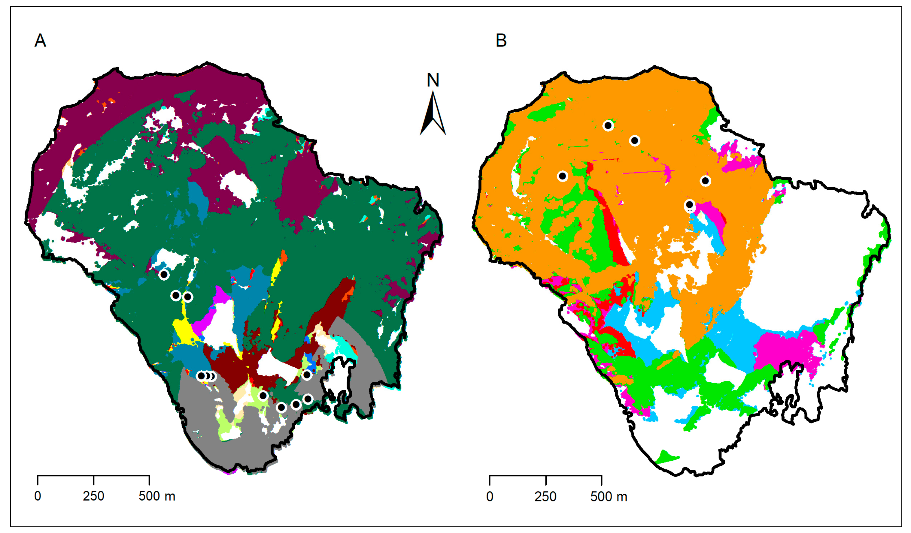
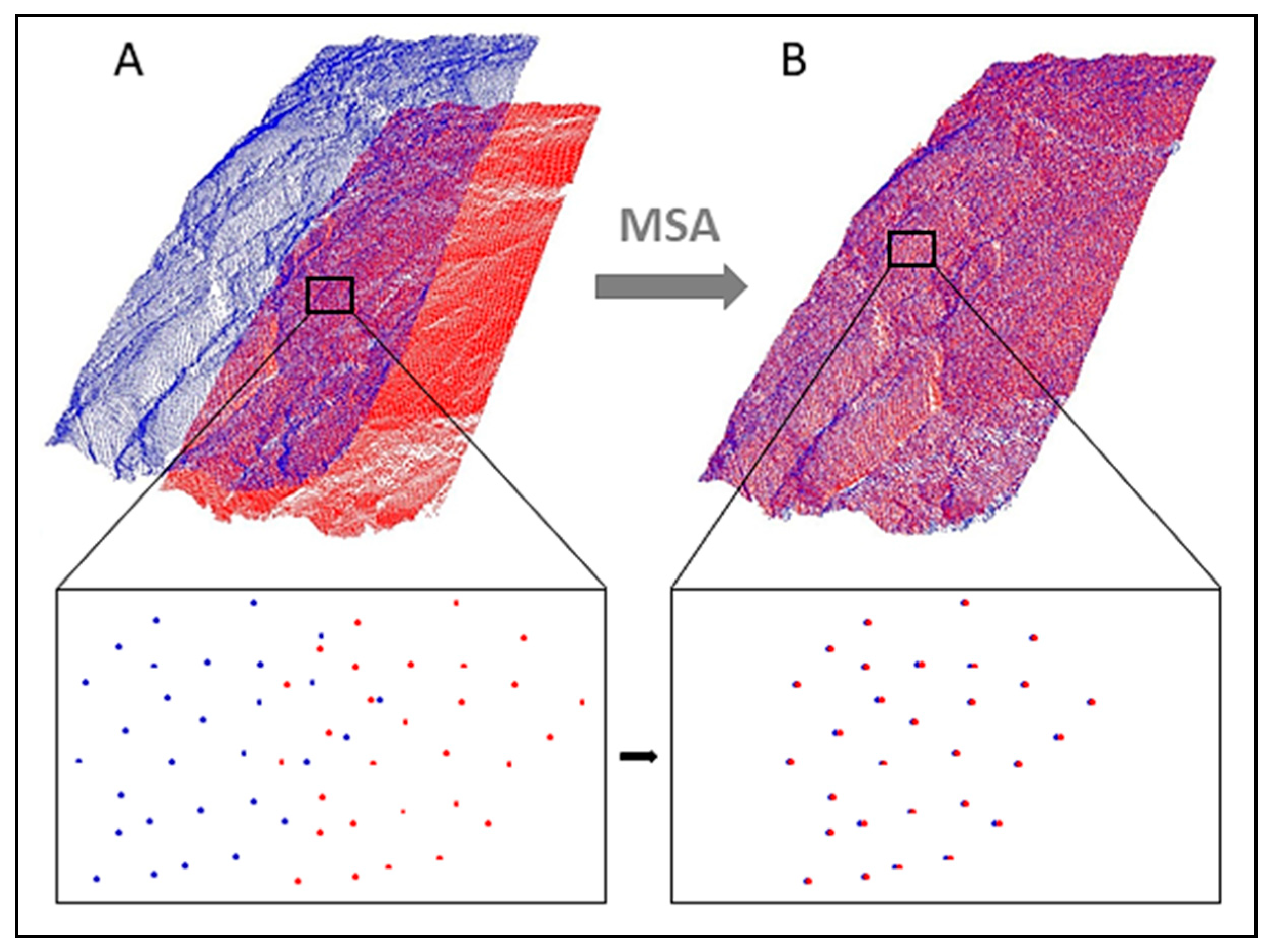
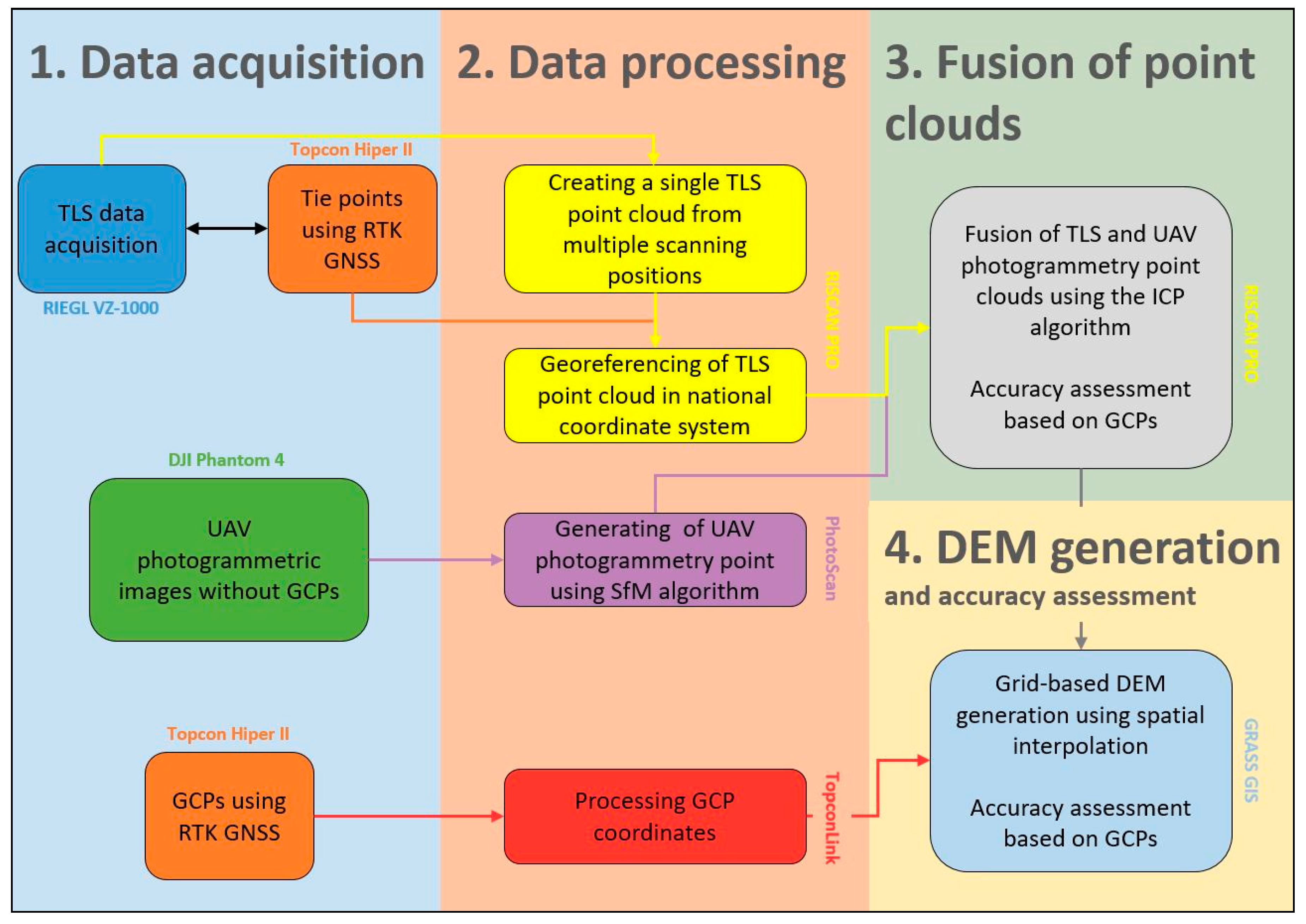
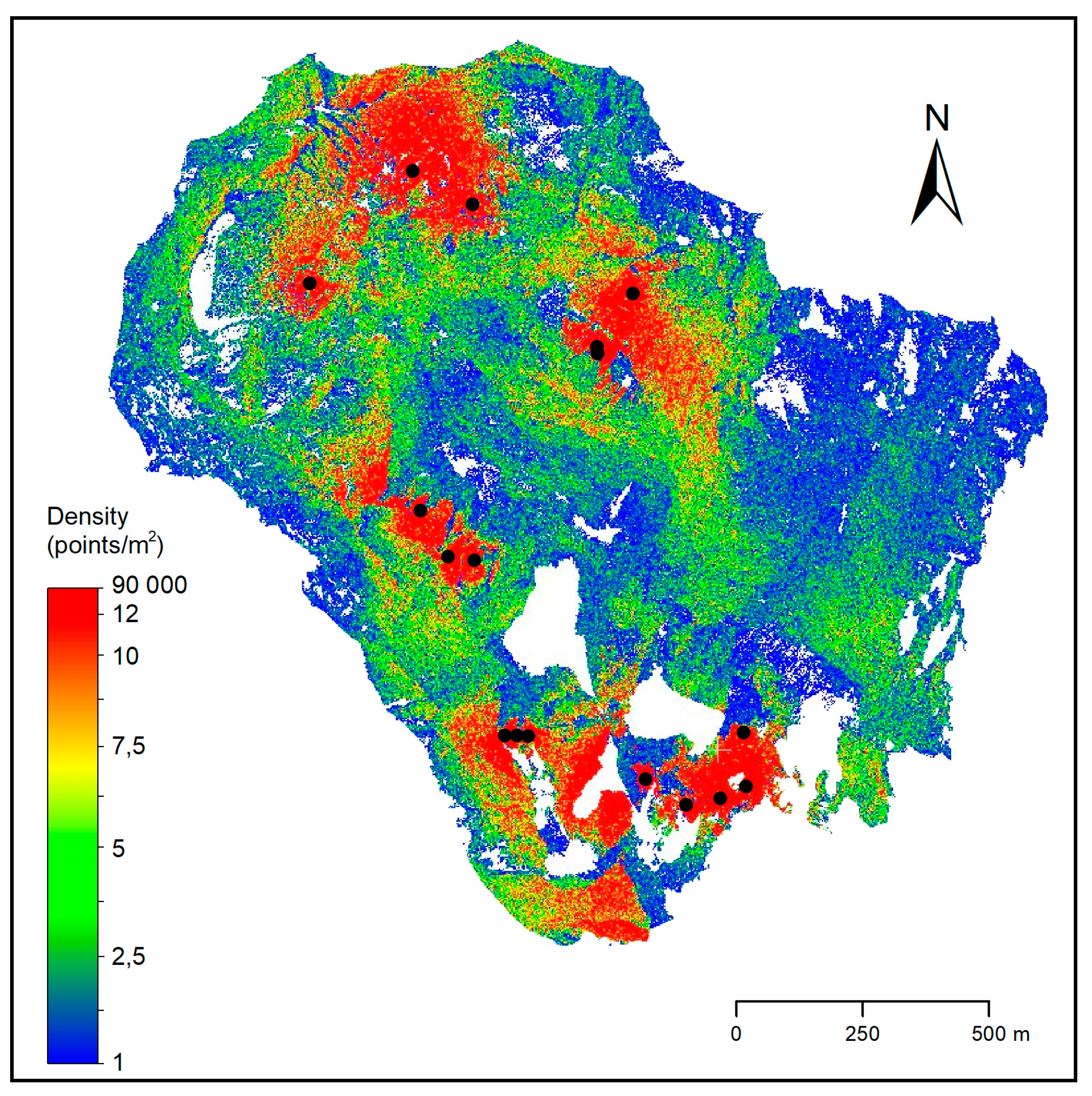
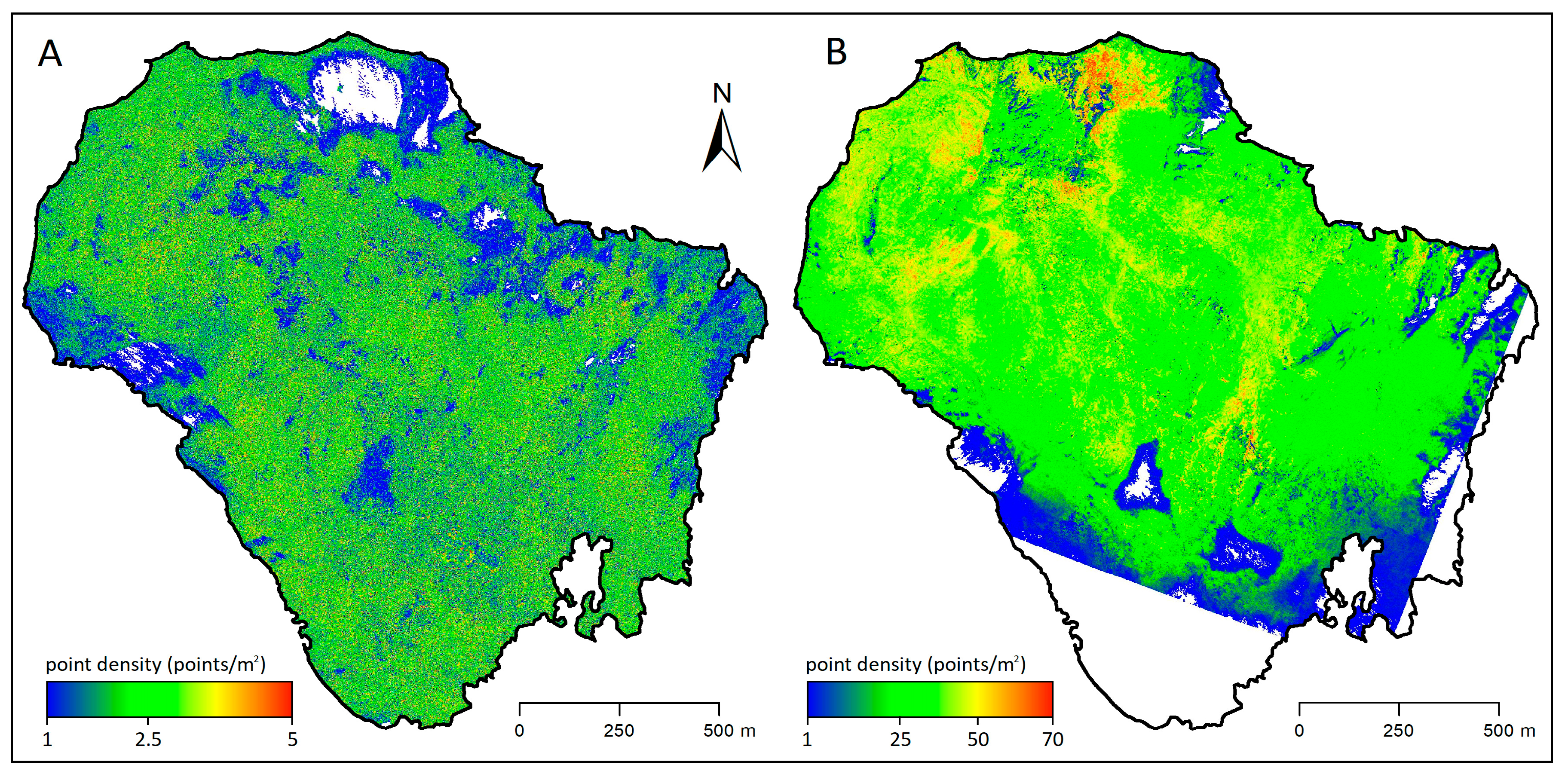
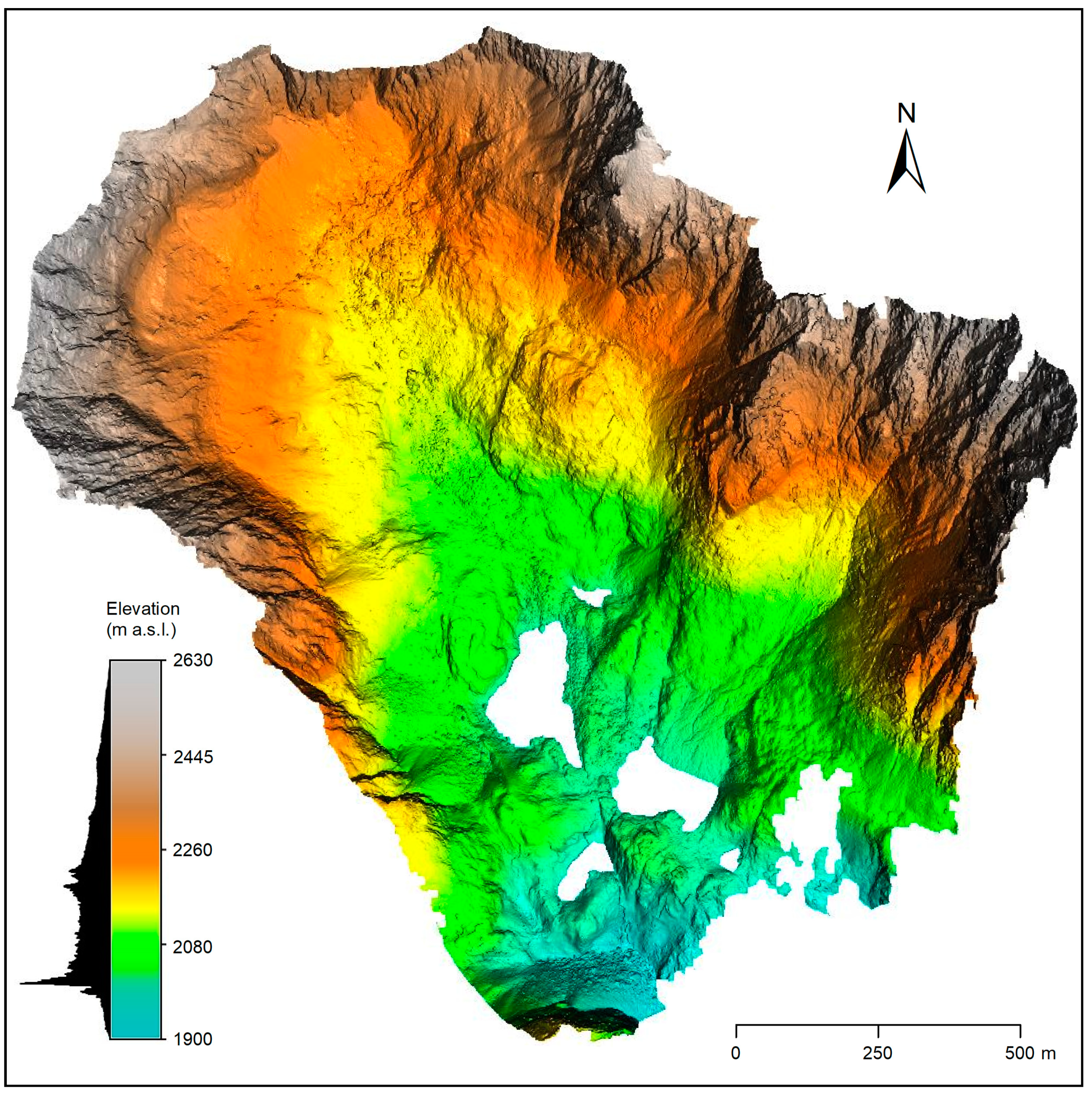
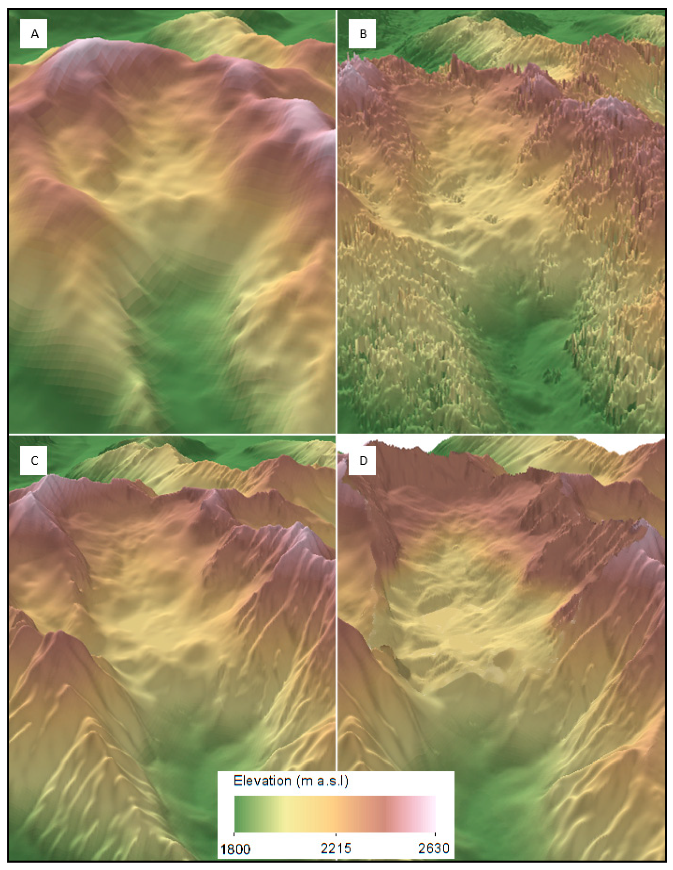
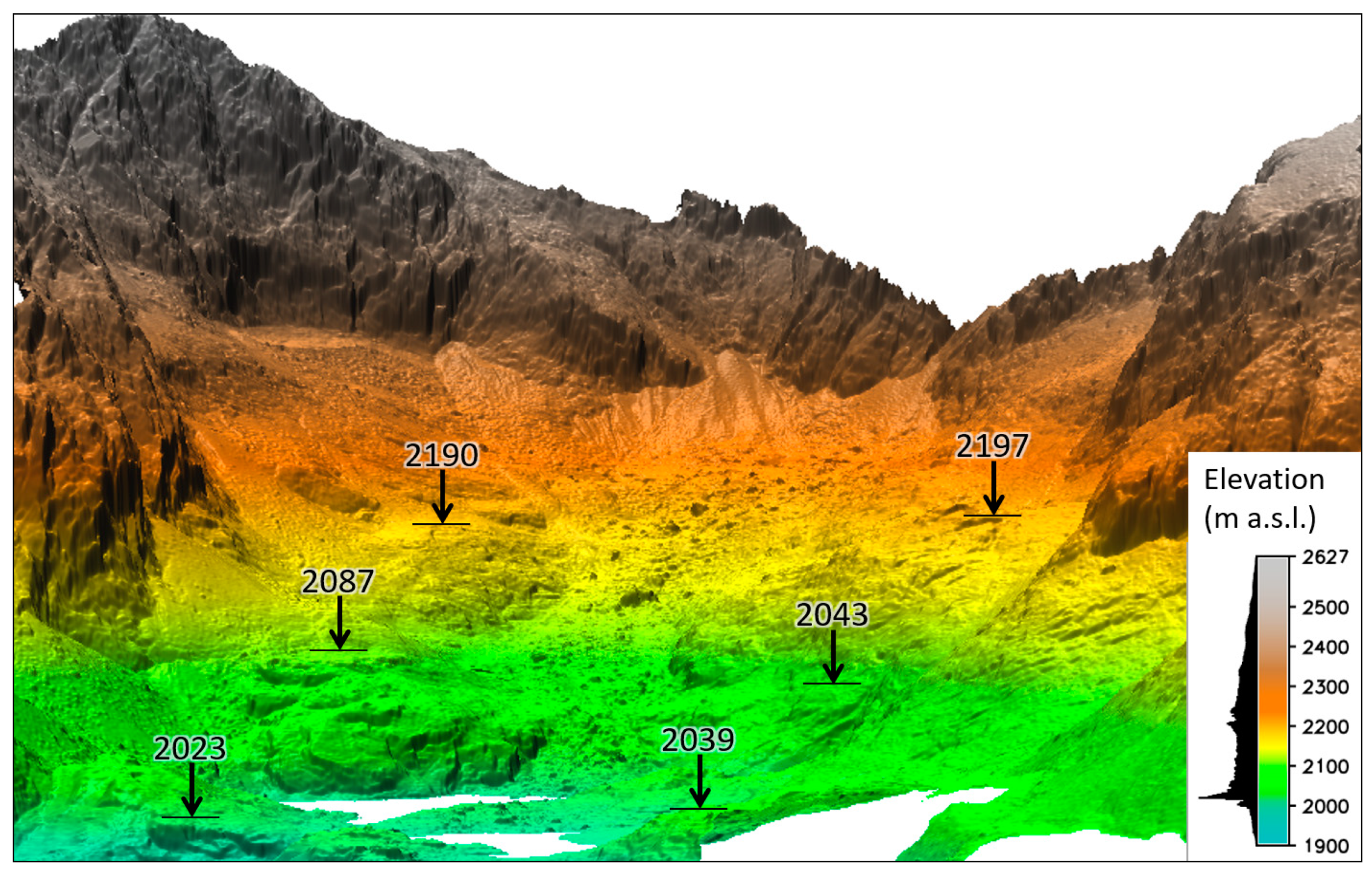
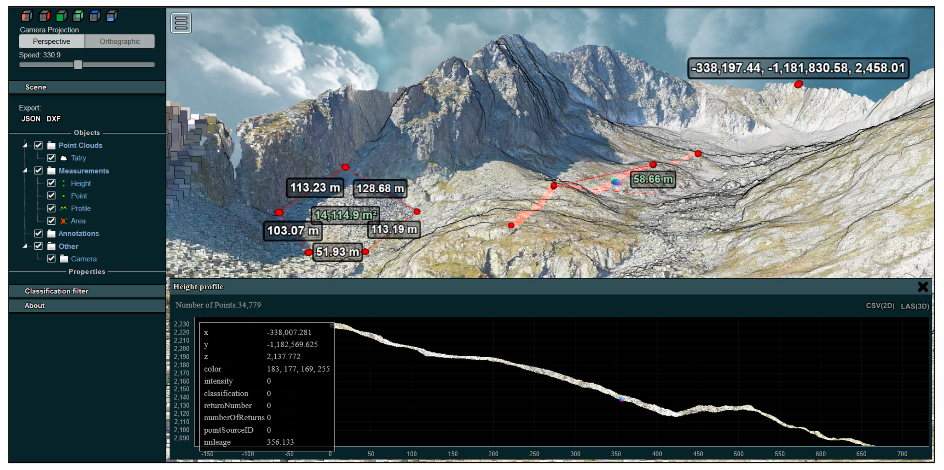
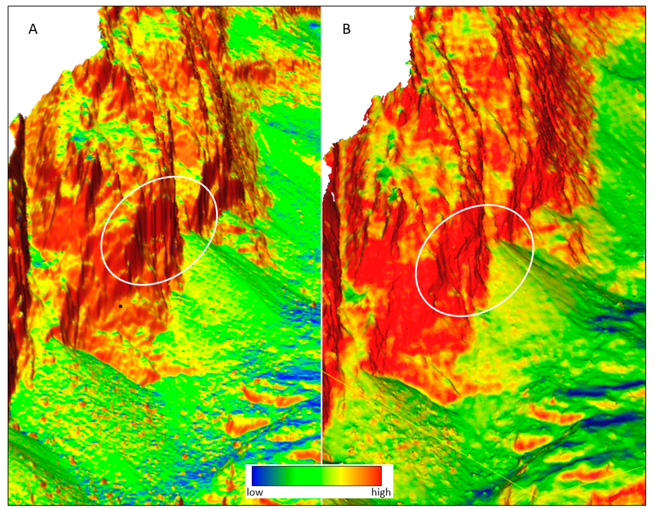
Table 1.
Summary statistics of cloud-to-cloud 3D distances between the GCPs and the final TLS-UAV-SfM point cloud and of the elevation differences between the GCPs and the final DEM (units in meters).
Table 1.
Summary statistics of cloud-to-cloud 3D distances between the GCPs and the final TLS-UAV-SfM point cloud and of the elevation differences between the GCPs and the final DEM (units in meters).
| Data | Final Point Cloud | Final DEM |
|---|---|---|
| Number of GCPs | 104 | 104 |
| Minimum | 0.003 | −2.137 |
| Maximum | 0.380 | 0.025 |
| Range | 0.377 | 2.162 |
| Mean | 0.114 | −0.461 |
| Mean of abs. values | 0.114 | 0.461 |
| Variance | 0.007 | 0.118 |
| Standard deviation | 0.086 | 0.342 |
| RMSE | 0.143 | 0.574 |
| 5th percentile | 0.011 | −1.114 |
| 1st quartile | 0.045 | −0.604 |
| Median | 0.102 | −0.366 |
| 3rd quartile | 0.170 | −0.245 |
| 95th percentile | 0.291 | −0.087 |
Table 2.
Summary statistics of vertical differences of SRTM, TanDEM-X and DMR3 DEM (DODs) calculated with respect to the TLS–UAV-SfM DEM for original resolutions of compared DEMs (elevation values in meters).
Table 2.
Summary statistics of vertical differences of SRTM, TanDEM-X and DMR3 DEM (DODs) calculated with respect to the TLS–UAV-SfM DEM for original resolutions of compared DEMs (elevation values in meters).
| Data | SRTM | TanDEM-X 12 m | DMR3 10 m |
|---|---|---|---|
| Number of DEM cells | 1940 | 18 634 | 20 645 |
| Minimum | −98.33 | −404.138 | −99.120 |
| Maximum | 85.56 | 95.123 | 53.971 |
| Range | 183.896 | 499.260 | 153.092 |
| Mean | −2.440 | −17.447 | −0.439 |
| Mean of abs. values | 14.044 | 21.364 | 4.447 |
| Variance | 449.728 | 2290.010 | 57.065 |
| Standard deviation | 21.207 | 47.854 | 7.554 |
| RMSE | 21.346 | 50.935 | 7.567 |
| 5th percentile | −36.134 | −128.525 | −10.311 |
| 1st quartile | −10.439 | −6.063 | −3.028 |
| Median | −3.365 | −0.267 | −0.367 |
| 3rd quartile | 5.059 | 1.113 | 1.935 |
| 95th percentile | 31.835 | 10.687 | 10.373 |
© 2019 by the authors. Licensee MDPI, Basel, Switzerland. This article is an open access article distributed under the terms and conditions of the Creative Commons Attribution (CC BY) license (http://creativecommons.org/licenses/by/4.0/).
Share and Cite
MDPI and ACS Style
Šašak, J.; Gallay, M.; Kaňuk, J.; Hofierka, J.; Minár, J. Combined Use of Terrestrial Laser Scanning and UAV Photogrammetry in Mapping Alpine Terrain. Remote Sens. 2019, 11, 2154. https://doi.org/10.3390/rs11182154
AMA Style
Šašak J, Gallay M, Kaňuk J, Hofierka J, Minár J. Combined Use of Terrestrial Laser Scanning and UAV Photogrammetry in Mapping Alpine Terrain. Remote Sensing. 2019; 11(18):2154. https://doi.org/10.3390/rs11182154
Chicago/Turabian StyleŠašak, Ján, Michal Gallay, Ján Kaňuk, Jaroslav Hofierka, and Jozef Minár. 2019. "Combined Use of Terrestrial Laser Scanning and UAV Photogrammetry in Mapping Alpine Terrain" Remote Sensing 11, no. 18: 2154. https://doi.org/10.3390/rs11182154
Note that from the first issue of 2016, this journal uses article numbers instead of page numbers. See further details here.