Evaluating Empirical Regression, Machine Learning, and Radiative Transfer Modelling for Estimating Vegetation Chlorophyll Content Using Bi-Seasonal Hyperspectral Images

Abstract

Different types of methods have been developed to retrieve vegetation attributes from remote sensing data, including conventional empirical regressions (i.e., linear regression (LR)), advanced empirical regressions (e.g., multivariable linear regression (MLR), partial least square regression (PLSR)), machine learning (e.g., random forest regression (RFR), decision tree regression (DTR)), and radiative transfer modelling (RTM, e.g., PROSAIL). Given that each algorithm has its own strengths and weaknesses, it is essential to compare them and evaluate their effectiveness. Previous studies have mainly used single-date multispectral imagery or ground-based hyperspectral reflectance data for evaluating the models, while multi-seasonal hyperspectral images have been rarely used. Extensive spectral and spatial information in hyperspectral images, as well as temporal variations of landscapes, potentially influence the model performance. In this research, LR, PLSR, RFR, and PROSAIL, representing different types of methods, were evaluated for estimating vegetation chlorophyll content from bi-seasonal hyperspectral images (i.e., a middle- and a late-growing season image, respectively). Results show that the PLSR and RFR generally performed better than LR and PROSAIL. RFR achieved the highest accuracy for both images. This research provides insights on the effectiveness of different models for estimating vegetation chlorophyll content using hyperspectral images, aiming to support future vegetation monitoring research.

1. Introduction

Vegetation biochemical and biophysical properties, such as chlorophyll content and leaf area index, are essential vegetation characteristics that influence plant physiological status, vegetation productivity, and ecosystem health [1,2]. As an example, chlorophyll controls the amount of solar radiation and CO₂ that a plant uses for photosynthesis, thus highly influencing vegetation photosynthetic capacity and productivity [3]. Investigation of vegetation properties is critical for understanding vegetation growth condition and supporting resource management [4]. Field measurements of vegetation properties are costly, labor-intensive, and limited to small areas [5]. In contrast, remote sensing is a low-cost and efficient tool for estimating vegetation properties and investigating their spatio-temporal variations over large areas [6,7]. Different approaches have been applied for estimating vegetation properties from remote sensing data, including conventional empirical regressions (i.e., linear regression (LR)), advanced empirical regressions (e.g., multivariable linear regression (MLR), partial least square regression (PLSR), principal component regression (PCR)), machine learning (e.g., random forest regression (RFR), decision tree regression (DTR), artificial neural networks (ANN)), and radiative transfer modelling (RTM, e.g., PROSPECT, PROSAIL) [5,8,9,10,11,12,13]. These approaches were developed using different theories and thus are expected to perform differently when estimating vegetation properties.

Previous research has attempted to compare various models for estimating vegetation properties. For instance, Powell et al. [14] compared RFR, reduced major axis regression, and gradient nearest neighbour imputation for estimating forest biomass using Landsat imagery. Darvishzadeh et al. [15] investigated PLSR and PROSAIL for retrieving grassland leaf area index (LAI) from HyMap data. Siegmann and Jarmer [16] evaluated performance of PLSR, support vector regression (SVR), and RFR for estimating wheat LAI using field-measured hyperspectral reflectance. Wang et al. [17] compared RFR, SVR, and ANN for investigating wheat biomass using multispectral HJ-CCD imagery. Reddy et al. [18] applied PLSR and RFR for modelling forest structural attributes (e.g., volume, tree height) using airborne multispectral imagery. Xing et al. [19] tested performance of PLSR, SVM, RFR, and ridge regression for estimating nutrition components (e.g., protein and sugar) in forage crops using a few field-based multispectral sensors and active sensors (e.g., laser). Yue et al. [13] examined ANN, MLR, DTR, PLSR, RFR, SVM, boosted binary regression tree (BBRT), and PCR for estimating wheat biomass using field-measured hyperspectral reflectance. In summary, most of these studies have compared advanced empirical regressions (e.g., PLSR, MLR) with machine learning methods (e.g., RFR, ANN), while less studies have compared these with two other commonly used approaches: conventional empirical regressions and radiative transfer modelling. The conventional empirical regression (e.g., LR using vegetation index) is the most widely used approach for retrieving vegetation information from remote sensing data owing to its easy application and fast computing. The advanced empirical regressions (e.g., PLSR) and machine learning approaches (e.g., RFR) are expected to outperform the conventional empirical regressions (e.g., LR) since they can use information from multiple predictor variables [20], however, it is unknown how much higher accuracy they can achieve. In many real-world practices, e.g., estimating crop properties in precision farming, the LR with acceptable accuracy is still preferred owing to its operational and computing advantages. Therefore, it is valuable to explore strategies for building well-performing LRs and comparing their accuracy with that of more advanced models. RTM is another approach used for investigating vegetation properties using remote sensing data. It describes the interaction of electromagnetic radiation with plants (reflection, transmission, absorption) using physical laws and simulates vegetation spectra at different wavelength ranges using vegetation biophysical and biochemical properties [21,22]. The RTM is a less often used approach due to model complexity and computing challenges. However, the RTM is physically-based, not sensor-, site-, or season-specific, and thus it is a more transferable approach than the empirical-based methods [5]. Therefore, it is valuable to compare RTM to other approaches and evaluate their accuracy and effectiveness.

Previous studies comparing different approaches have mainly utilized multispectral images or ground based hyperspectral reflectance data, while few studies have applied hyperspectral images to evaluate the performance of different models. The hyperspectral imagery records the spectral signal of ground features in hundreds of narrow spectral bands over a large area. The huge amount of spectral and spatial (i.e., image textural) information may influence the performance of different models, which has not been fully explored in previous studies. Moreover, most of previous studies have utilized single-date images for the comparison of different approaches, while less have used multi-temporal data. The phenological variations of vegetation (e.g., changes from homogeneous green canopies in the middle growing season to heterogeneous canopies with mixed green and senescent vegetation in the late growing season) also potentially influence the effectiveness of different models. It is thus critical to investigate if the models perform differently for images acquired from different seasons. In addition, most of previous model comparison studies attempted to investigate vegetation biophysical properties [14,15,16,17,18], such as vegetation structure and biomass, while few have focused on estimating vegetation biochemical properties (e.g., vegetation chlorophyll content). Different spectral features need to be utilized for investigating vegetation biochemical properties and model performance may vary depending on which spectral features are used. For instance, spectral signals in blue, red, and NIR ranges are critical for estimating canopy chlorophyll content (e.g., signals in blue and red capturing chlorophyll absorption features and signals in NIR reflecting vegetation density information). Models capable of selecting and utilizing spectral variables in these ranges can potentially achieve higher estimation accuracy. In this study, bi-seasonal high-spatial resolution hyperspectral images were acquired by a helicopter-based imaging system and utilized for estimating vegetation canopy chlorophyll content with different models. Specifically, LRs, PLSR, RFR, and a modified PROSAIL, which represent conventional empirical regression, advanced empirical regression, machine learning, and RTM, respectively, were selected and compared. Different types of information, such as vegetation indices (VIs), reflectance of each band, principal components (PCs), and textural variables were extracted from the hyperspectral images and applied into different models as predictor variables.

LR is the most widely used approach for estimating vegetation properties from remote sensing data [4]. One common practice is to establish a LR between targeted vegetation properties (e.g., chlorophyll content) and remote sensing variables (e.g., VIs) using sampling data, and then applying this LR for predictive purposes. A large number of broadband or narrowband VIs have been developed in previous studies to retrieve vegetation properties, such as the widely used Normalized Difference Vegetation Index (NDVI), Soil-Adjusted Vegetation Index (SAVI), and Atmospherically Resistant Vegetation Index (ARVI) [23,24,25,26]. Previous studies have also compared these VIs and evaluated their performance for estimating various vegetation properties (e.g., chlorophyll content, biomass) in different ecosystems (e.g., forests, grasslands, and croplands) [4,5,17,27,28,29,30]. In this research, 29 VIs that performed well in previous studies for estimating vegetation canopy chlorophyll content were selected and further evaluated [28,30]. In addition to VIs, previous studies indicated that image PCs can provide important information for investigating vegetation properties [31,32]. Therefore, PCs were also tested as predictor variables in LR for estimating vegetation chlorophyll content.

To estimate vegetation properties, LR is relatively easy to build in comparison with more advanced regression models and LR generally performs well with appropriate VIs and training samples (e.g., selecting VIs from previous studies, collecting samples in a wide data range). However, there are several problems associated with LR for the retrieval of vegetation properties, such as saturation of some VIs (e.g., NDVI for dense green canopies), being highly affected by sample data (e.g., extreme values), and VIs influenced by environment factors (e.g., soil background, view geometry, atmospheric condition) [33,34,35]. Advanced empirical regressions, such as PLSR, have been developed and utilized to deal with these problems and improve the stability of regression models [13,16]. PLSR is a bi-linear calibration method using data compression technique that reduces the number of collinear predictor variables to a few non-correlated latent variables [18,35]. These latent variables are generated to maximize information content from the original variables and to optimize their explanatory power for predictions [36]. PLSR is considered as an efficient method for feature extraction and dimension reduction without losing much information [18,37]. It combines features of principal component regression and stepwise multivariable regression, and is capable of tackling some common problems in regression models, such as collinearity, data noise, and over-fitting [13,37,38,39]. PLSR has been used in previous studies for estimating vegetation LAI, biomass, or nitrogen content [8,35,39,40]. In this study, PLSR was tested to estimate canopy chlorophyll content.

Random Forest is an ensemble modelling technique that builds a forest with a large number of regression trees using bootstrapped training data [41,42]. It is a robust and widely used prediction model for regression and classification [12,43]. It has many advantages over other regression models, such as being able to handle thousands of input variables and running efficiently on a large dataset, not being sensitive to noise or over-fitting, handling the collinearity problem, requiring a minimal number of parameters, and making no distribution assumptions about the predictor or response variables [13,17,44]. One essential feature of random forest is that the importance of predictor variables can be evaluated in the model, which is essential for researchers to understand the contributions of different variables to the regression or classification model [44]. This variable importance is assessed based on how much the prediction accuracy decreases when a variable is permuted while the others are left unchanged [45,46]. Random forest has been widely applied in the remote sensing field for classification [43,47], however, it has been less used for regression to estimate vegetation properties [17,33,34]. A few existing studies include estimating biomass [17], vegetation structure [44], and water content [48]. In this study, RFR is examined to investigate its performance at estimating vegetation canopy chlorophyll content.

PROSAIL is one of the most-widely applied canopy-level radiative transfer models, describing the spectral and directional variation of canopy reflectance in the solar domain [11]. It integrates the leaf-level PROSPECT model and canopy-level SAIL model. Specifically, it passes the output leaf reflectance and transmittance of the PROSPECT model into the SAIL model to simulate the whole spectro-directional canopy reflectance. Therefore, it links the canopy reflectance with leaf biochemical contents (e.g., leaf pigments, water, and dry matter), canopy architecture (e.g., LAI, leaf angle distribution, and relative leaf size), soil properties, illumination conditions, and viewing geometry [49]. The PROSAIL model has been applied successfully in different homogeneous ecosystems (e.g., forests and crops) for estimating vegetation biophysical and biochemical properties (e.g., LAI, leaf chlorophyll content) [11,50,51,52]. However, it was found to struggle with simulating spectra of heterogeneous canopies with mixed green and senescent vegetation [22,53], likely because the leaf-level PROSPECT model cannot sufficiently simulate spectra of senescent leaves [54]. A modified PROSPECT that is capable of tackling this problem was developed and applied in this study to generate a modified PROSAIL [54]. This modified PROSAIL is compared to regression models for estimating vegetation canopy chlorophyll content.

Canopy heterogeneity (i.e., mixed green and senescent vegetation) is an essential vegetation biophysical characteristic of an ecosystem, especially for heterogeneous grasslands or wetlands. Such heterogeneity may influence the retrieval of vegetation properties using remote sensing. As mentioned previously, high heterogeneity was found to bring considerable challenges to the PROSAIL model for simulating vegetation spectra in a grassland area [22,53]. In addition, it also affected the accuracy of empirical models (e.g., PLS) for estimating vegetation properties [55]. The influence of vegetation heterogeneity on the performance of different models (RTM-based or empirical models) for the estimation of vegetation properties have rarely been explored in previous research. Many studies estimating vegetation properties using different models have focused on homogeneous ecosystems, such as crops and forests, while less focused on heterogeneous ecosystems, such as grasslands and wetlands [14,56,57,58]. In this study, bi-seasonal hyperspectral images were acquired in a grassland area, which capture vegetation information with different level of heterogeneities. Specifically, one image was acquired in the middle growing season (i.e., June) that featured by homogeneous green canopies and the other image was acquired in the late growing season (i.e., August) that exhibited high heterogeneity (e.g., a mixture of green and senescent vegetation). These two images were used for evaluating effects of heterogeneity on the performance of models.

This study compared the performance of LR, PLSR, RFR, and a modified PROSAIL model for retrieving vegetation chlorophyll content from bi-seasonal hyperspectral images in a heterogeneous grassland area. Different image features, including VIs, spectral reflectance, PCs, and image textural variables were extracted from the images, aiming to acquire different types of information from the images and optimize the performance of different models. Contributions of different types of variables to different models (e.g., importance values of these variables) were also evaluated. Different optimization techniques were used in PLSR and RFR models for improving their performance. A modified PROSAIL model, which can accurately simulate reflectance of heterogeneous canopies, was adopted in this study and compared to other models. Factors influencing model performance were also discussed in order to provide insights with other researchers on the selection and optimization of different models.

2. Material and Methods

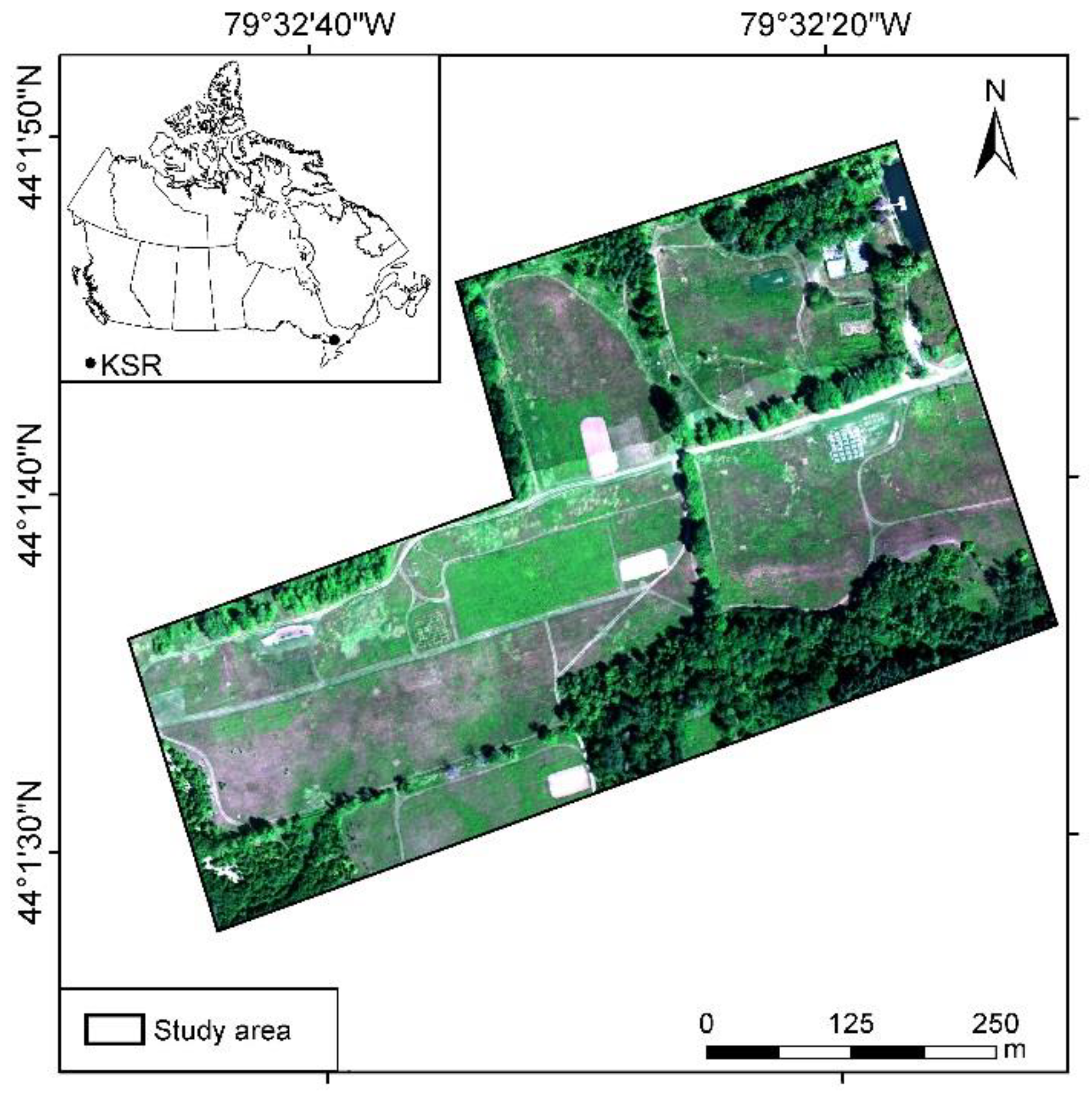
2.1. Study Area

This research was performed at Koffler Scientific Reserve (KSR), located in Southern Ontario, Canada (Figure 1). Grasslands in KSR mainly consist of temperate tall grasses with a height ranging from 10 to 50 cm during the growing season (May to September) [59]. Dominant grass species in this area are Awnless brome (Bromus inermis), Fescue (Festuca rubra L.), Goldenrod (Solidago canadensis L.), and Milkweed (Asclepias L.). The climate type in this area is temperate continental, with a mean temperature ranging from −10 °C (February) to 30 °C (July), and precipitation ranging from 20 mm (March) to 100 mm (July) [60]. The soil in this area is typically grey-brown podzolic soil.

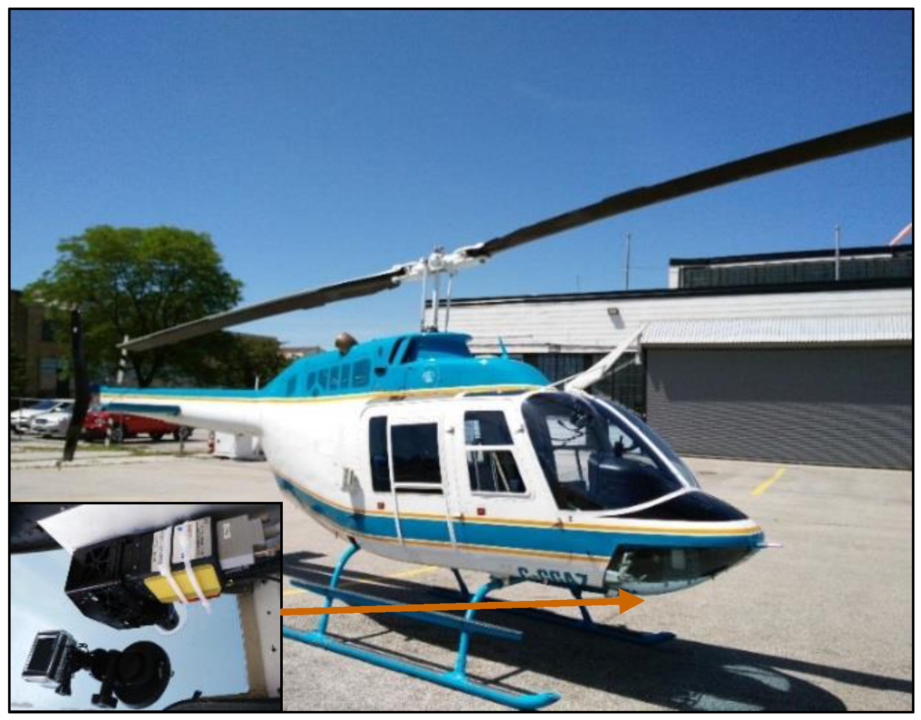
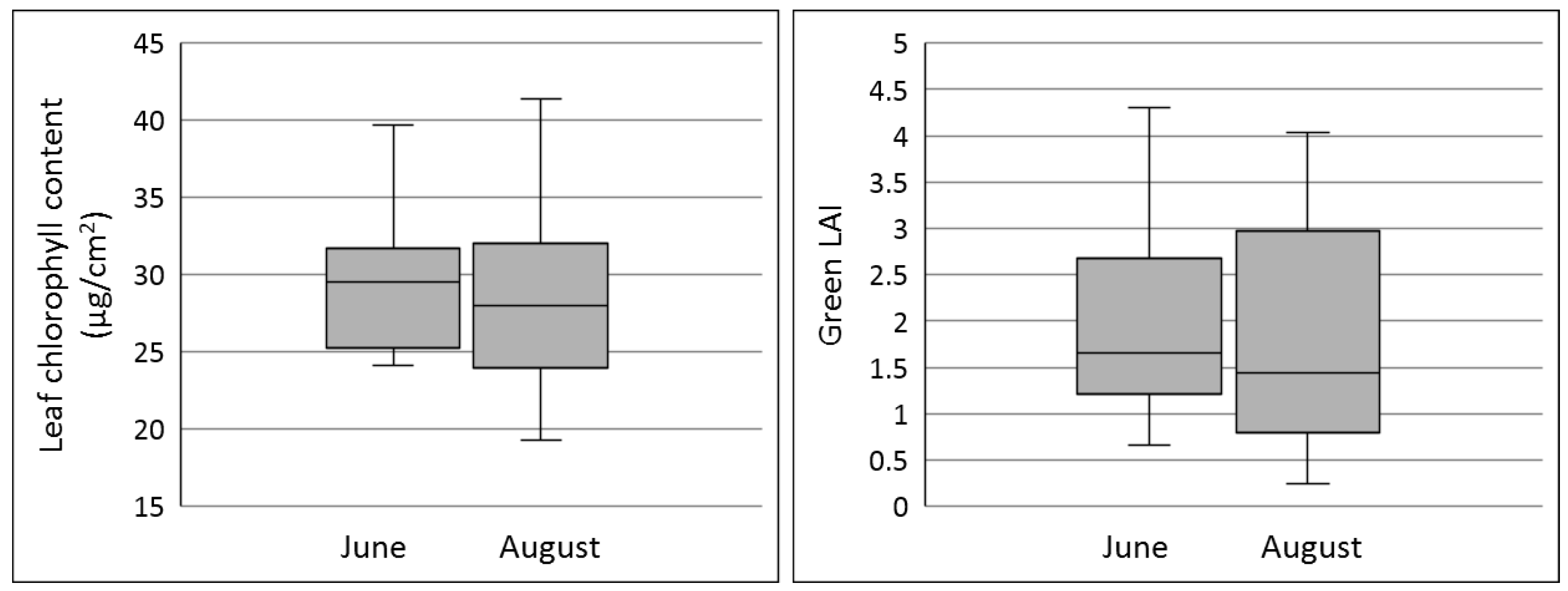
2.2. Hyperspectral Imagery Collection and Field Survey

Hyperspectral images were collected using a Micro-HyperSpec (Headwall Photonics Inc., Boston, MA, USA) that was mounted on a manned helicopter (Figure 2). This sensor is capable of collecting spectral signals in more than 300 bands ranging from 400 to 1000 nm. Two flight missions were conducted around noon on 14 June (middle growing season) and 26 August, 2016 (late growing season), aiming to capture the homogeneous and heterogeneous features of this grassland ecosystem, respectively. The weather conditions on both days were sunny and clear. The flights were operated at a height of 250 m and acquired imagery with a spatial resolution of 30 cm. The acquired images were radiometrically and geometrically corrected using SpectralView that was provided by the sensor manufacturer. The images were further atmospherically corrected in ENVI (Exelis Visual Information Solutions, Boulder, CO, USA) using an empirical line method [61,62]. Lastly, the images were resampled to 301 bands with a 2 nm interval from 400 to 1000 nm.

Field surveys were performed simultaneously with the flight missions. A total of 29 study sites were pre-selected in the study area for the field survey in June. The selection of sites was dependent on vegetation growing conditions, species composition, and topographic conditions. An extra five study sites were added for the field survey in August due to the increased variety of vegetation canopy features. The location of each site was obtained using a highly accurate Trimble GeoExplorer GPS (Trimble Navigation Limited, Sunnyvale, CA, USA). Field data collected at the study sites included spectral reflectance, LAI, vegetation height, species composition, and canopy photos. The spectral reflectance data were collected using an ASD spectroradiometer FieldSpec 3 in the range of 350–2500 nm (Analytical Spectral Devices Inc., Boulder, CO, USA). LAI was measured using an AccuPAR LP-80 ceptometer (Decagon Devices, Inc., Pullman, Washington, WA, USA). Leaf samples for each site were also collected and transported to a laboratory for measuring leaf reflectance and chlorophyll content. Leaf reflectance was acquired using Plant Probe (Analytical Spectral Devices, Inc., Boulder, CO, USA) that was connected to the ASD FieldSpec spectroradiometer, following the protocol provided by [63] and [64]. The measured reflectance data were used for evaluating the simulation results from radiative transfer models. Leaf chlorophyll was extracted using N, N-dimethylformamide (DMF) following a protocol proposed by [65]. Canopy chlorophyll content was then calculated using leaf chlorophyll content times LAI of green vegetation (i.e., green LAI) [2,5,66,67,68]. For the survey in June, the green LAI equals to the field-measured canopy LAI since the canopies were homogeneous green vegetation. For the survey in August, the canopies were heterogeneous with mixed green and senescent vegetation. The green LAI was calculated using field-measured canopy LAI times the percentage of green vegetation in this canopy. This percentage (e.g., 20%, 55%, or 100%) was manually estimated in the field using a quadrat (0.5 × 0.5 m). Statistics of measured leaf chlorophyll content and green LAI is shown in Figure 3. Correlations between canopy chlorophyll content and green LAI and correlations between canopy chlorophyll and leaf chlorophyll were calculated to evaluate the influence of green LAI and leaf chlorophyll on the variations of canopy chlorophyll.

2.3. Methods and Model Parameter Settings

LR, PLSR, RFR, and a modified PROSAIL were selected for comparison to evaluate their performance of estimating canopy chlorophyll content. Details of each model are described in below sections. A leave-one-out cross validation (LOOCV) was used for validating the models [13,33] and the coefficient of determination (R²), together with root mean square error (RMSE), were calculated and applied to describe performance of different models [13].

2.3.1. Linear Regression

LRs were built using different predictor variables to estimate canopy chlorophyll content. In this study, 29 narrowband VIs (

Table 1. Narrowband vegetation indices selected in this research. (R in the formula indicates reflectance, values indicate wavelength in nm).

Index	Full Name	Formula	References
BGI	Blue/Green Pigment Index	$R_{450}/R_{550}$	[70]
DVI	Difference Vegetation Index	$R_{800}-R_{680}$	[71]
GI	Greenness Index	$R_{554}/R_{677}$	[70]
GVI	Greenness Vegetation Index	$(R_{682}-R_{553})/\left(R_{682}+R_{553}\right)$	[72]
MCARI1	Modified Chlorophyll Absorption Ratio Index 1	$\left[\left(R_{750}-R_{705}\right)-0.2\left(R_{750}-R_{550}\right)\right]\left(R_{750}/R_{705}\right)$	[73]
MCARI2	Modified Chlorophyll Absorption Ratio Index 2	$\frac{1.5\left[1.2\left(R_{800}-R_{550}\right)-2.5\left(R_{670}-R_{550}\right)\right]}{\sqrt{{\left(2R_{800}+1\right)}^2-\left(6R_{800}-5\sqrt{R_{670}}\right)}-0.5}$	[74]
MRENDVI	Modified Red Edge Normalized Difference Vegetation Index	$\left(R_{750}-R_{705}\right)/\left(R_{750}+R_{705}-2R_{445}\right)$	[75]
MSAVI	Modified Soil Adjusted Vegetation Index	$0.5\left[2R_{800}+1-\sqrt{{\left(2R_{800}+1\right)}^2-8\left(R_{800}-R_{670}\right)}\right]$	[25]
mSR1	Modified Simple Ratio 1	$\frac{\frac{R_{800}}{R_{670}}-1}{\sqrt{\frac{R_{800}}{R_{670}}}+1}$	[76]
mSR2	Modified Simple Ratio 2	$\frac{\left(\frac{R_{750}}{R_{705}}\right)-1}{\sqrt{\left(\frac{R_{750}}{R_{705}}\right)+1}}$	[73]
mSR3	Modified Simple Ratio 3	$\left(R_{750}-R_{445}\right)/\left(R_{705}-R_{445}\right)$	[75]
MTCI	MERIS Terrestrial Chlorophyll Index	$\left(R_{754}-R_{709}\right)/\left(R_{709}-R_{681}\right)$	[77]
MTVI	Modified Triangular Vegetation Index	$\frac{1.5\left[1.2\left(R_{800}-R_{550}\right)-2.5\left(R_{670}-R_{550}\right)\right]}{\sqrt{{\left(2R_{800}+1\right)}^2-6R_{800}+5{\left(R_{670}\right)}^{0.5}-0.5}}$	[74]
NDRE	Normalized Difference Red-edge index	$\left(R_{790}-R_{720}\right)/\left(R_{790}+R_{720}\right)$	[78]
NDVI	Normalized Difference vegetation index	$\left(R_{682}-R_{553}\right)/\left(R_{682}+R_{553}\right)$	[72]
OSAVI1	Optimized Soil Adjusted Vegetation Index 1	$1.16\left(R_{800}-R_{670}\right)/\left(R_{800}+R_{670}+0.16\right)$	[79]
OSAVI2	Optimized Soil Adjusted Vegetation Index 2	$1.16\left(R_{750}-R_{705}\right)/\left(R_{750}+R_{705}+0.16\right)$	[73]
PPR	Plant Pigment Ratio	$\left(R_{550}-R_{450}\right)/\left(R_{550}+R_{450}\right)$	[80]
PRI	Photochemical Reflectance Index	$\left(R_{570}-R_{539}\right)/\left(R_{570}+R_{539}\right)$	[81]
RDVI	Renormalized Difference vegetation index	$\frac{R_{800}-R_{670}}{\sqrt{R_{800}+R_{670}}}$	[82]
RENDVI	Red Edge Normalized Difference Vegetation Index	$\left(R_{750}-R_{705}\right)/\left(R_{750}+R_{705}\right)$	[75,83]
REPI	Red Edge Position Index	$700+40\left({\mathsf{\rho }}_{\mathrm{REP}}-R_{700}\right)/\left(R_{740}-R_{700}\right)$ ${\mathsf{\rho }}_{\mathrm{REP}}=0.5\left(R_{670}+R_{780}\right)$	[84]
RRVI	Reciprocal Reflectance-based Vegetation Index	$R_{750-800}/R_{695-740}-1$	[85]
RGI	Red/Green Index	$R_{690}/R_{550}$	[70]
SPVI	Spectral Polygon Vegetation Index	$0.4\left[3.7\left(R_{800}-R_{670}\right)-1.2\left|R_{530}-R_{670}\right|\right]$	[86]
SR	Simple Ratio	$R_{800}/R_{675}$	[71]
TSAVI	Transformed Soil Adjusted Vegetation Index	$\frac{\alpha \left(R_{875}-\alpha R_{680}-\beta \right)}{\left[R_{680}+\alpha \left(R_{875-\beta }\right)+0.08\left(1+{\alpha }^2\right)\right]}$ $\alpha =1.062\beta =0.022$	[26]
VREI	Vogelmann Red Edge Index	$\left(R_{734}-R_{747}\right)/\left(R_{715}+R_{726}\right)$	[87]
ZM	Zarco and Miller	$R_{750}/R_{710}$	[51]

) that performed well in previous studies for estimating canopy chlorophyll content were used as predictor variables [28,30]. In addition, a preliminary test showed that PCs of all spectral bands can contribute to the estimation of canopy chlorophyll content and they were also used in previous studies for retrieving vegetation properties [69]. Therefore, top 10 PCs that can cover the majority of spectral band information (i.e., PC1 to PC10) were calculated and selected as predictor variables. Total 39 predictor variables were used to build LRs and their performances were later evaluated.

2.3.2. Partial Least Square Regression

The partial least square regression in Python with Scikit-Learn library was applied in this study [88]. The 29 VIs and 10 PCs used in LRs were also used as predictor variables in PLSR. In addition, since spectral bands may also contribute to the model prediction, reflectance values of the 301 bands were thus also used as predictor variables. These variables were named as Re + wavelength, such as Re550 and Re800. Moreover, image textural features (e.g., entropy, homogeneity) contain essential information describing vegetation structural patterns and spatial variations, which potentially can also contribute to the estimation of vegetation properties [55,89]. Therefore, eight textural variables, including mean, variance, homogeneity, contrast, dissimilarity, entropy, second moment, and correlation, were calculated for selected spectral bands in ENVI using a kernel size of 5 × 5 (close to the size of a study site). These textural variables were named as b + wavelength–variable type, such as b800-mean and b740-entropy. Calculating eight textural variables for all of the spectral bands are computationally challenging with much information overlap since some spectral bands are correlated. Therefore, seven bands that are most frequently used for calculating the VIs listed in Table 1, were selected for calculating image textural variables. Details of these seven bands can be found in Section 3.1. Overall, there were 29 VIs, 10 PCs, 301 reflectance, and 56 textural variables used as predictor variables in the PLSR.

The PLSR is capable of dealing with a large number of predictor variables by converting them into a few latent variables. The predicted residual error sum of squares (PRESS) statistics was applied to identify the optimal number of latent variables in PLSR that has the lowest model error. Since some predictor variables may not contribute to the regression model or may bring in noise, a backward feature elimination method was applied to eliminate the less promising variables and identify the model that achieves the highest accuracy [19,48]. The variable importance on projection (VIP) values were calculated in PLSR to evaluate effects of variables on the regression model [90]. The least important variables (i.e., with lowest VIP values) were progressively deleted and the model was consequently rebuilt. Thus, a series of models were established and then also validated. The model with the lowest RMSE was regarded as the best performing model [48].

2.3.3. Random Forest Regression

The random forest regression in Python with Scikit-Learn library was utilized in this study [88]. There are three essential parameters need to be determined in the RFR model: number of trees to grow (Ntree, default 100), number of predictor variables to test at each splitting node (Mtry, default all variables), and node size that is the minimum number of samples required to be at a leaf node (Nodesize, default 1) [34,44]. The Mtry and Nodesize values were kept as default as suggested in previous studies, while the Ntree was tested using 100, 200, 500, 1000, and 2000 to optimize the model performance (i.e., lowest RMSE) [33,34,41,46].

The predictor variables used in PLSR, including VIs, reflectance, PCs, and textural variables, were also used in RFR. Importance values of all predictor variables were calculated in RFR [44], and then the backward feature elimination method was applied to RFR to progressively remove the least important variables [19,33,34,41]. The model with the lowest RMSE was regarded as the optimal model.

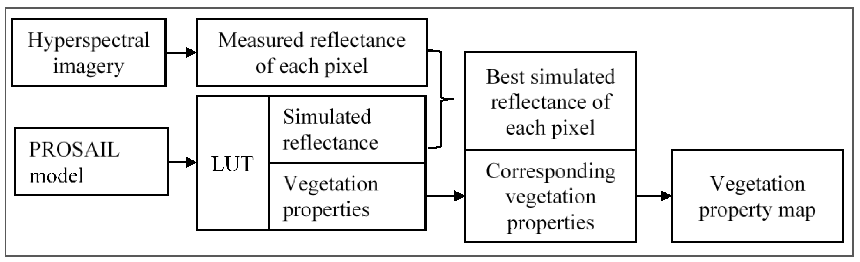
2.3.4. A Modified PROSAIL

The PROSAIL model was downloaded from this link (http://teledetection.ipgp.jussieu.fr/prosail/, accessed in June 2017, version 5B) and was operated in Matlab [11]. This original PROSAIL was found to suffer when simulating the spectra of heterogeneous canopies [22,53], likely because the leaf-level PROSPECT model cannot sufficiently simulate spectra of senescent leaves [54]. Therefore, a modified PROSPECT that is capable of tackling this problem was developed and applied in this study to generate a modified PROSAIL [54]. Parameters in PROSAIL include leaf chlorophyll content, leaf water content, leaf area index, solar and view geometry, and soil reflectance [9,11,54]. Vegetation canopy reflectance was extracted from hyperspectral imagery. A lookup table approach (LUT) was applied as the inversion method to estimate vegetation properties from the canopy reflectance data [50,91]. A brief workflow of the inversion is shown in Figure 4. A LUT was defined using all possible values within a value range for each parameter in the PROSAIL model. This value range was determined with prior knowledge from the literature [9,11,54]. For instance, the leaf chlorophyll content has a range of 0~100 µg/cm² and the leaf water content (i.e., equivalent water thickness) has a range of 0~0.05 cm. Then, the model calculated all possible combinations of values from different parameters and simulated reflectance correspondingly. This method covers all types of leaves and canopy structures, thus generating a dataset including all possible reflectance. With the measured canopy reflectance from hyperspectral imagery, a global search was performed in the LUT to identify parameter combinations that yield the best fit between measured and forward-simulated vegetation spectra. At last, vegetation properties, i.e., optimal parameter combinations, including leaf chlorophyll content and LAI, were determined.

3. Results and Discussion

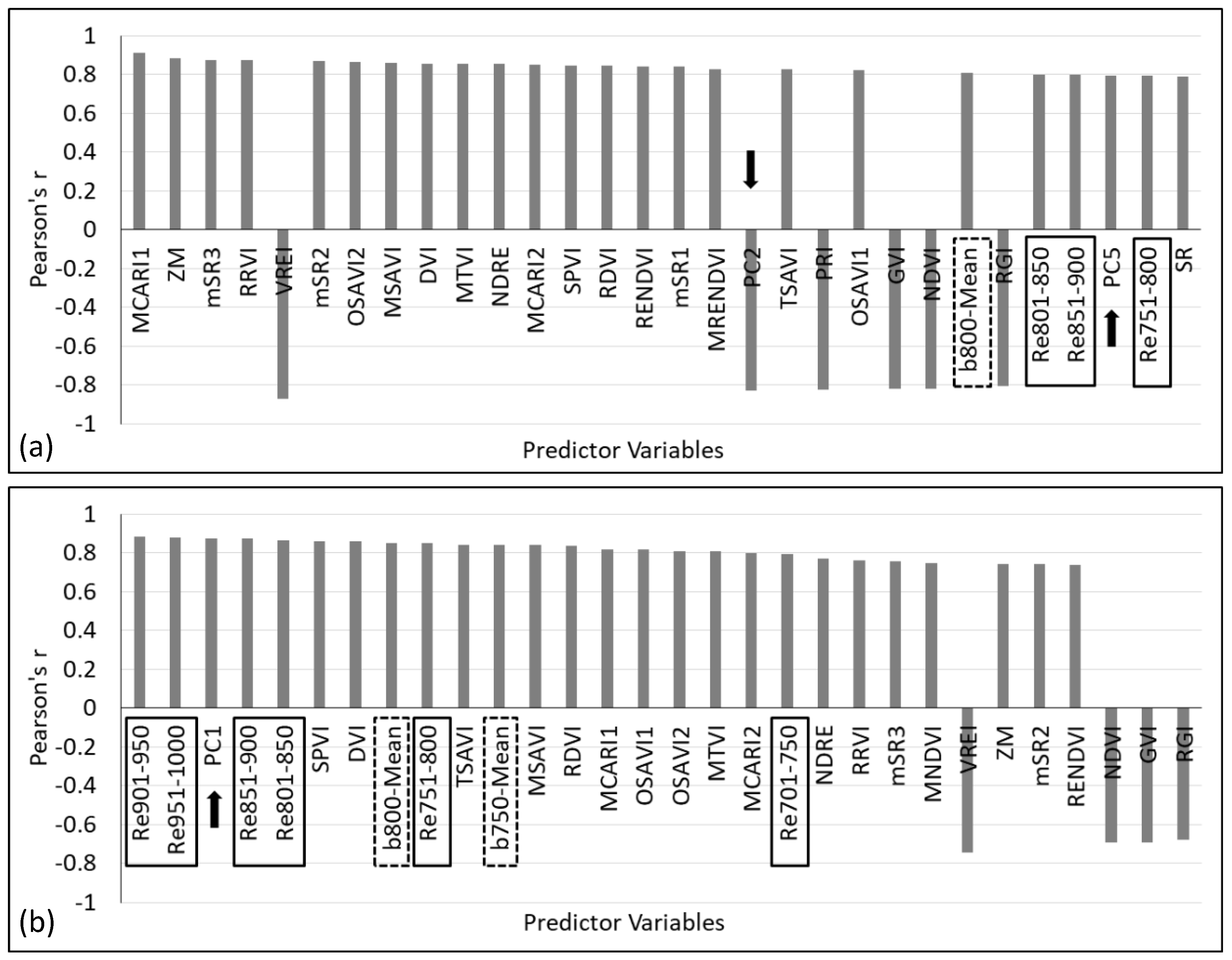
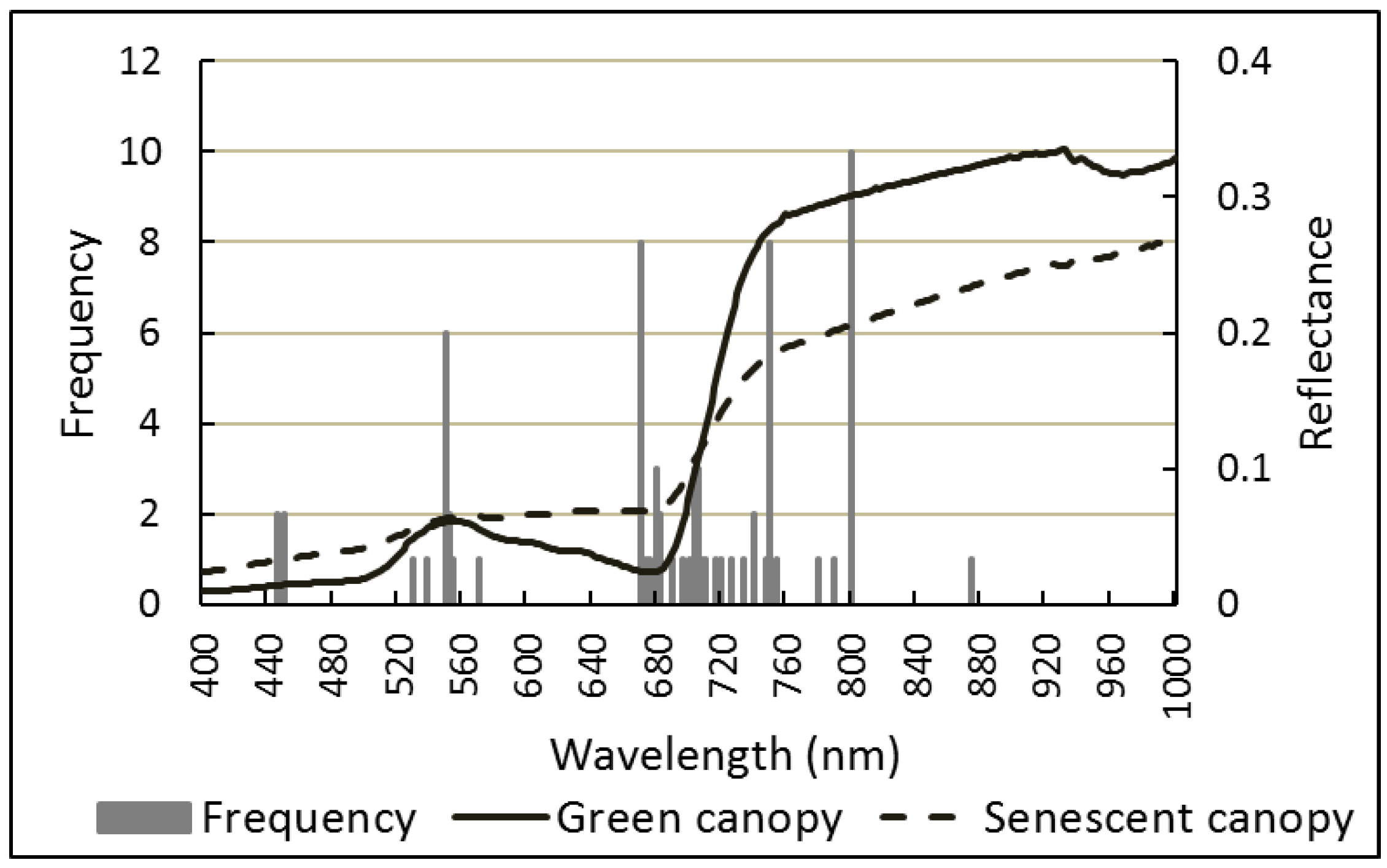
3.1. Analysis of Predictor Variables

The correlations between each predictor variable (e.g., VIs, reflectance, PCs, and textural variables) and canopy chlorophyll content were first examined and the top 30 strongest ones (or groups of neighboring reflectance) are illustrated in Figure 5. These top 30 strongest correlations have Pearson’s r values around 0.8. The corresponding top 30 predictor variables include VIs, PCs, reflectance, and textural variables, indicating these different types of variables can all potentially contribute to the estimation of canopy chlorophyll. For the June image that captured homogeneous green vegetation, the top 17 variables are all VIs that have Pearson’s r values over 0.8, such as MCARI1, ZM, and mSR3 (Figure 5a). The VIs were selected based on their good performance in previous studies for estimating canopy chlorophyll and thus their strong correlations were expected in this study. Several other types of predictor variables, such as PC2, b800-Mean, and Re801–850, have only slightly weaker correlations with canopy chlorophyll than the VIs.

To further understand which bands were used in the VIs listed in Table 1 and identify the most frequently used ones that may be important for estimating canopy chlorophyll, the frequencies of different bands used in VIs were calculated and plotted in Figure 6. The top four most often used bands are centered around 550, 670, 750, and 800 nm, which are in the high reflection range in green, the deep absorption portion in red, the increasing reflection part in red-edge, and the peak reflection range in NIR, respectively (Figure 6). The reflection strength in green and red is influenced by leaf chlorophyll, while the strength in NIR is related to leaf structure and LAI (i.e., canopy density) [28]. Bands in the blue ranges, such as those around 450 nm, also have high frequencies. In addition, the bands in the red-edge range, such as those between 700 and 750 nm (e.g., 704 nm, Figure 6), are also often used in VIs. It is reported that using red-edge bands in VIs can minimize the saturation problem of the indices, reduce the influences of atmospheric and water absorption and background noise, and mitigate the vegetation surface scattering and bidirectional reflectance distribution function (BRDF) effects [33]. Several VIs that have used red-edge bands, such as MCARI1, ZM, and mSR3, show very strong correlations with the canopy chlorophyll (Figure 5). Overall, seven bands, including 450,550,670,680,704,750, and 800 nm, are more frequently used in the VIs, indicating their importance for estimating chlorophyll. Images of these seven bands are utilized for producing textural variables mentioned in Section 2.3.2.

For the August image that is featured by senescent canopies (i.e., with mixed green and senescent vegetation and low canopy chlorophyll), the VIs have weaker correlations with canopy chlorophyll than the other types of predictor variables (Figure 5b). For instance, the top five variables (or groups of variables) are reflectance (e.g., Re901–950) and PC1. Only three VIs (i.e., SPVI, DVI, and TSAVI) are among the top 10. This indicates that the VIs have weaker correlations with chlorophyll of senescent canopies than that of green canopies. Many VIs are built based on low reflectance in the red and high reflectance in the NIR (as green canopy reflectance shown in Figure 6) to highlight the green vegetation information and chlorophyll signal. However, for senescent canopies, the reflectance is higher in red and lower in NIR (as senescent canopy reflectance shown in Figure 6). The effectiveness of VIs for highlighting the chlorophyll information of senescent canopies is lower and thus they have relatively weaker correlations compared to that of green canopies. In contrast, reflectance in the NIR (e.g., 800–1000 nm) has strong correlations with chlorophyll of senescent canopies (Figure 5b). This is probably because the reflectance strength in NIR is highly affected by LAI and the canopy chlorophyll content was calculated using LAI. Canopies with high LAI show high reflectance in NIR and also have high canopy chlorophyll content, which thus leads to the strong correlation between reflectance in NIR and the canopy chlorophyll content. The results suggest that it is important to evaluate the influence of LAI and leaf chlorophyll content on the variations of canopy chlorophyll content. We found that the correlations between LAI and canopy chlorophyll are very strong (e.g., Pearson’s r of 0.96 for the June survey and 0.97 for the August survey), while that between leaf chlorophyll and canopy chlorophyll are much weaker (e.g., Pearson’s r of 0.31 for the June survey and 0.28 for the August survey). These results demonstrated that LAI has much stronger influence on the variation in canopy chlorophyll content than the leaf chlorophyll content.

3.2. Optimization of PLSR and RFR

The importance of each predictor variable was evaluated in the PLSR and RFR, respectively, and a backward feature elimination method was used to remove less important variables from the model with the aim of identifying the best performing PLSR and RFR (i.e., with the lowest RMSE). The selected variables for the optimal PLSR and RFR of the June or August image (hereafter named PLSR-June, RFR-June, PLSR-August, and RFR-August) are listed in

Table 2. Selected variables in the optimal partial least square regression (PLSR) and random forest regression (RFR) for June and August images, respectively. Variables are grouped by types (e.g., vegetation indices (VIs), PCs). If a large number of variables of one type were selected, only the top five (e.g., with the highest importance in the model) are listed as examples.

	June Image		August Image
	PLSR	RFR	PLSR	RFR
Selected Variables	VIs: mSR3 VREI MTCI MCARI1 REPI (Total 27)   Reflectance: Re628-Re1000 (Total 167)   PCs: PC1, PC2, PC4, PC5   Textural: b550-Homogeneity b670-Second Moment b704-Entropy b750-Mean b800-Mean (Total 16)	VIs: NDRE RENDVI ZM RRVI MRENDVI (Total 14)   Reflectance: Re502   PCs: PC5   Textural: b680-Mean	VIs: SPVI DVI TSAVI MSAVI RDVI (Total 11)   Reflectance: Re714-Re1000 (Total 144)   PCs: PC1   Textural: b800-Meanb 750-Mean	VIs: TSAVI DVI NDRE MCARI1 MSAVI (Total 7)   Reflectance: Re802-Re1000 (Total 24)   PCs: PC3   Textural: b800-Mean b680-Correlation

. Different types of variables, including VIs, reflectance, PCs, and textural variables, are all among the selected variables of different models, indicating they can all contribute to model predictions.

Comparing the number of selected variables in PLSR and RFR, the PLSR needs to select more variables than the RFR does to achieve the optimal performance. For instance, the PLSR-June selected 27 VIs,167 reflectance, 4 PCs, and 16 textural variables to reach the highest accuracy, while the RFR-June selected 14 VIs, 1 reflectance, 1 PC, and 1 textural variable to achieve the best performance. Similar results can be found for the PLSR-August and RFR-August. This is because the PLSR and the RFR use different techniques to evaluate variable importance in the model and then select the variables based on their importance. Specifically, the PLSR considers the predictive power of variables when converting them to latent variables [36,90]. Therefore, the PLSR selected a large number of variables to gain the maximum predicting power, even when these variables may be correlated (e.g., the 167 reflectance in PLSR-June and the 144 reflectance in PLSR-August are intercorrelated, respectively). In contrast, the RFR selects the best performing variable for splitting nodes and growing trees and rates it as more important in the model [17,46]. Other variables that are correlated with this one will have limited contribution to the model and thus are rated as less important. Therefore, compared to PLSR, a smaller number of predictor variables are needed in the RFR model to achieve optimal model performance.

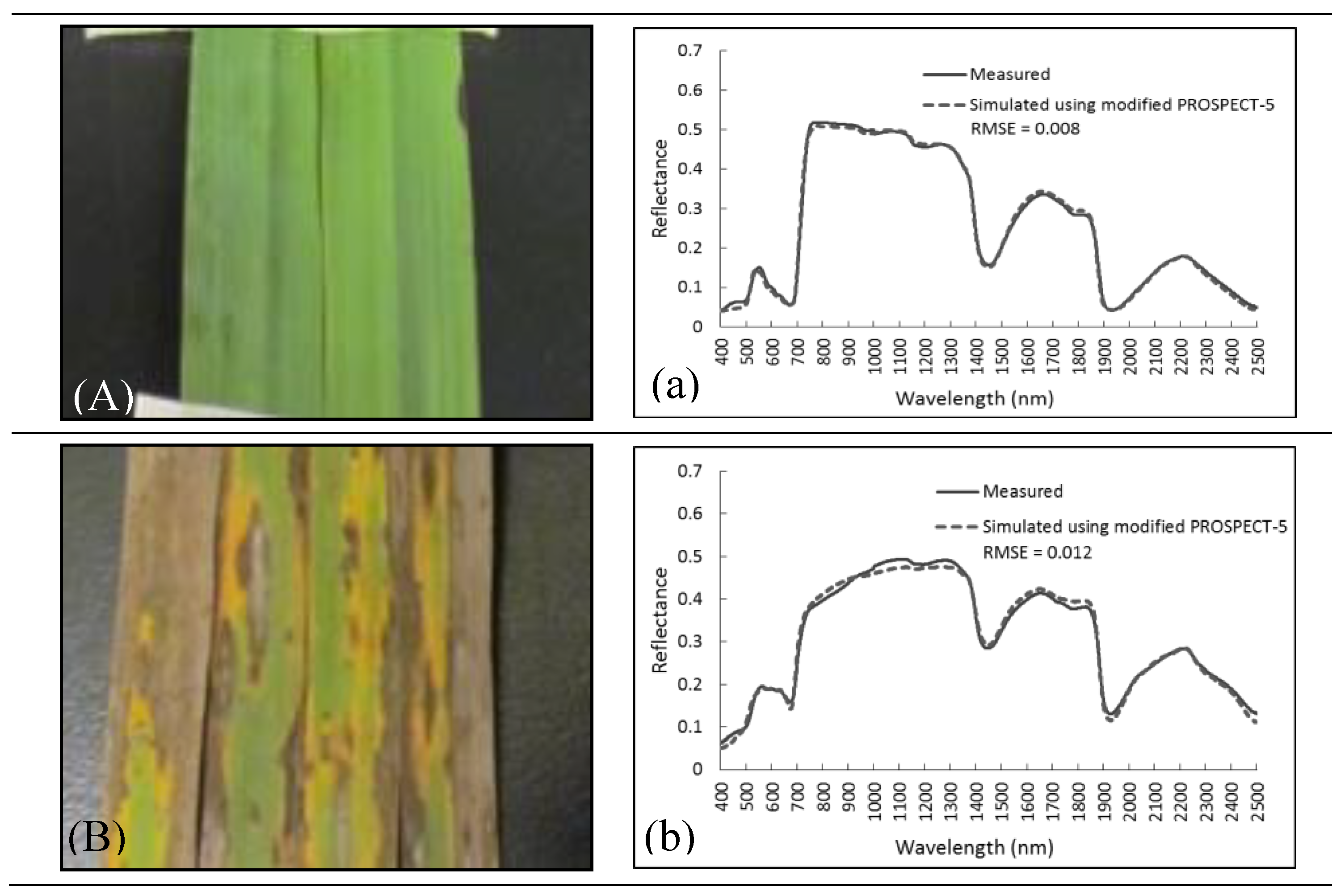
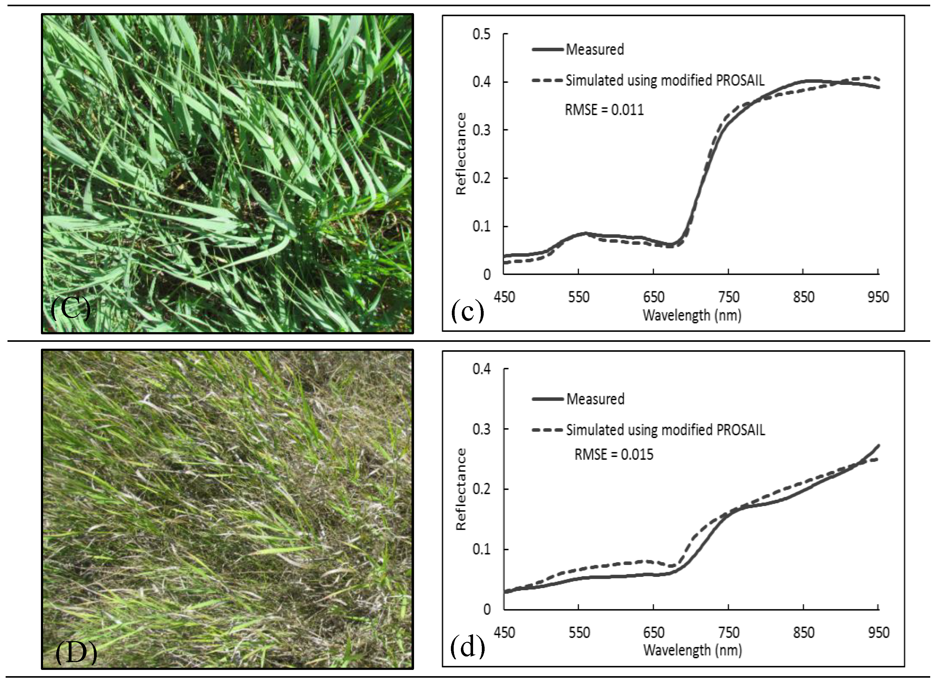
3.3. Forward Simulation Using PROSAIL

A modified PROSAIL model, which integrated a modified PROSPECT-5 model and SAIL model, was used for simulating vegetation spectra (e.g., leaf and canopy reflectance) and estimating vegetation properties (e.g., leaf chlorophyll content, LAI). The modified PROSPECT-5 model worked well for simulating reflectance of different types of leaves (e.g., green and senescent), achieving an average RMSE of 0.009 with a standard deviation of 0.004. Examples of leaf spectral simulations are shown in Figure 7a,b. The modified PROSAIL model also performed well for simulating reflectance of both green and mixed canopies, achieving an average RMSE of 0.029 with a standard deviation of 0.018. Examples of canopy spectral simulations are shown in Figure 7c,d. The effectiveness of PROSAIL for estimating vegetation properties are evaluated in the next sections.

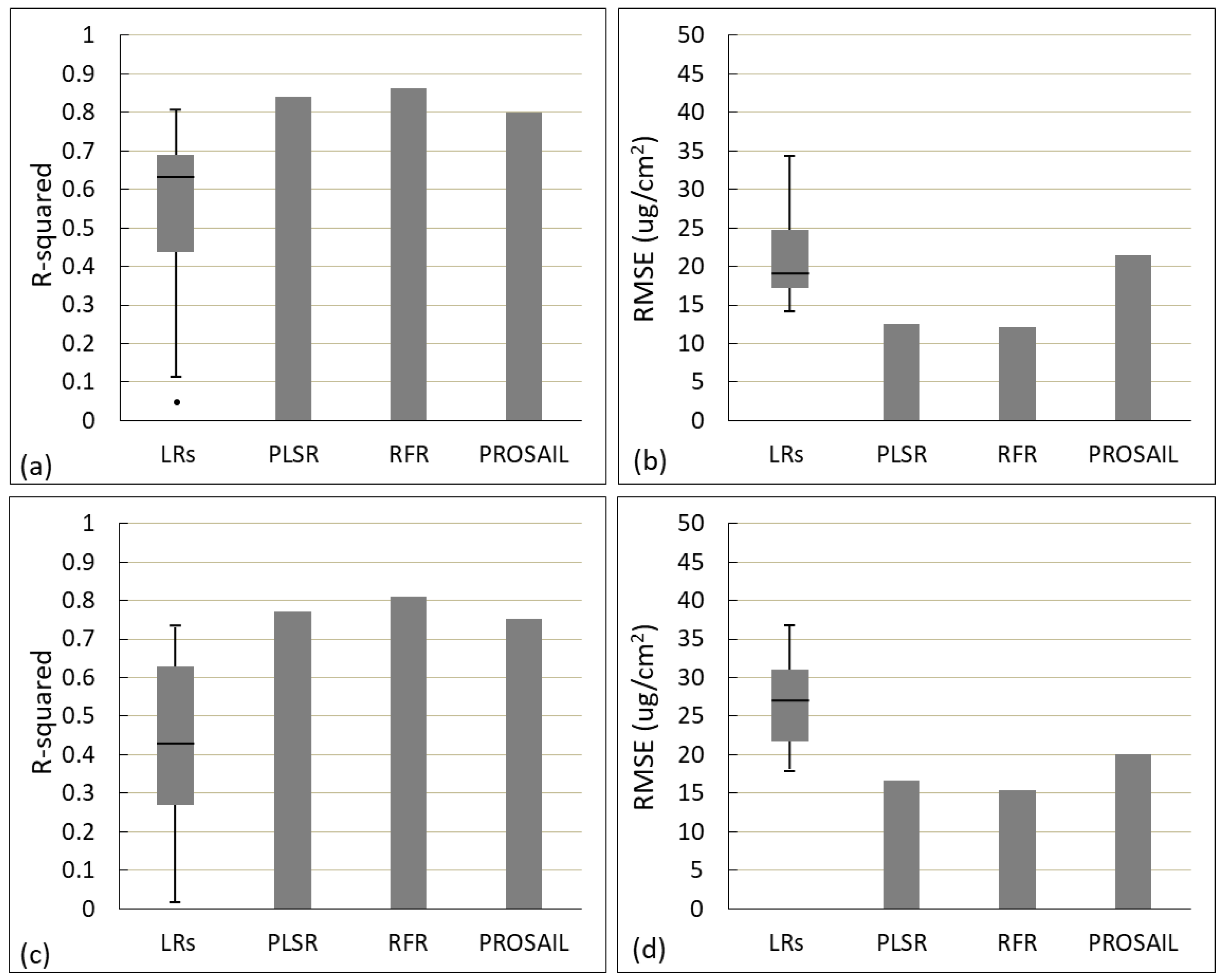
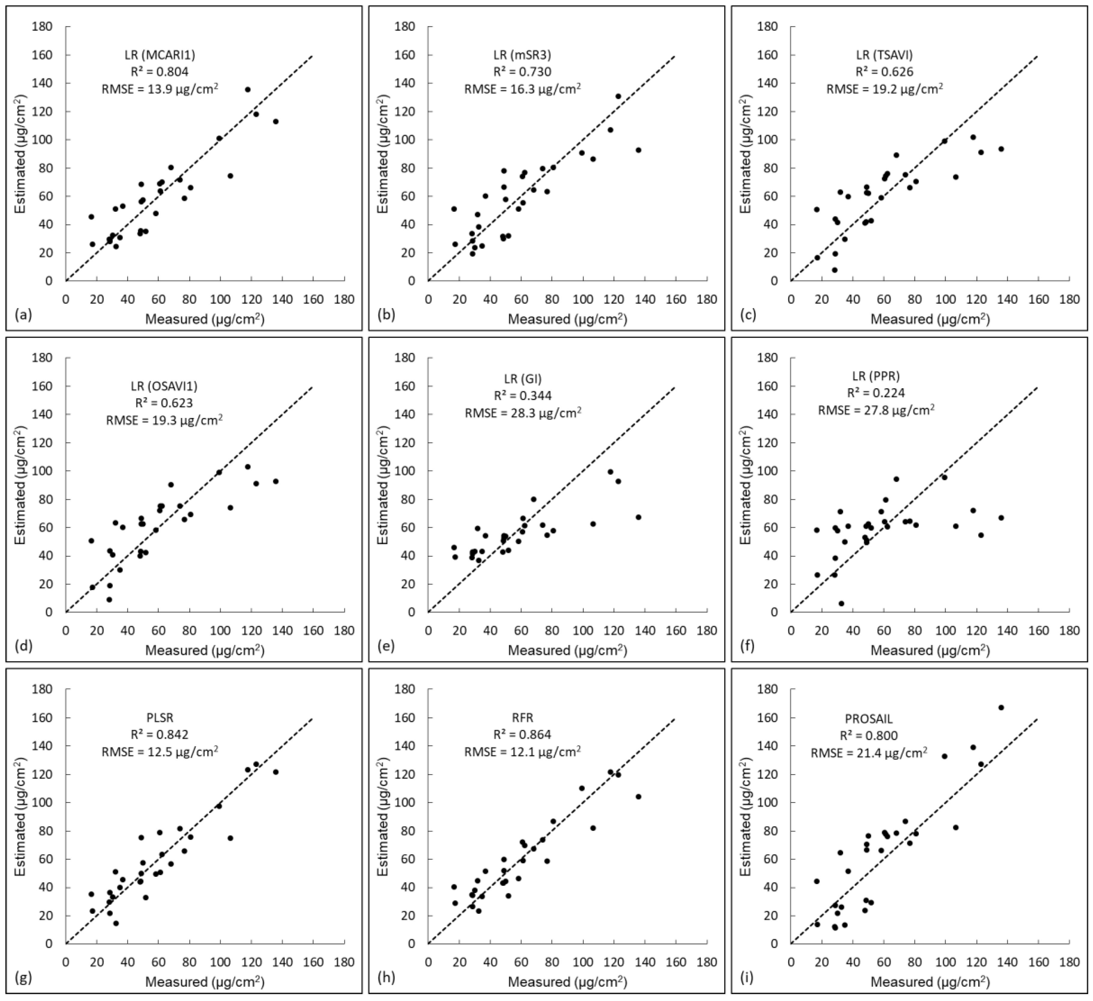
3.4. Result Comparison of Different Methods

LR, PLSR, RFR, and PROSAIL were utilized for estimating canopy chlorophyll content from images acquired in June and August, respectively. The validation results, including R² and RMSE, are shown in Figure 8. 39 LRs were built using 29 VIs and 10 PCs, and their accuracy values are described in boxplots in Figure 8. Overall, the best performing LRs, along with PLSR, RFR, and PROSAIL achieved good accuracies, such as R² ~ 0.82 and RMSE ~ 15.0 µg/cm² for the June image and R² ~ 0.75 and RMSE ~ 17.0 µg/cm² for the August image. The estimation accuracy for the August image is slightly lower than that of the June image, which is possibly due to vegetation senescence and reduced canopy chlorophyll content. Different models also have different performances for estimating canopy chlorophyll. For the June image, half of LRs achieved R² > 0.6 and RMSE < 20.0 µg/cm² (Figure 8a,b). A few top performing LRs included the ones using MCARI1 (R² = 0.80, RMSE = 13.9 µg/cm²), ZM (R² = 0.75, RMSE = 15.7 µg/cm²), and mSR3 (R² = 0.73, RMSE = 16.3 µg/cm²). For the August image, effectiveness of LRs are obviously lower than that for the June image. Only half of LRs achieved R² values higher than 0.4 and RMSE lower than 26.0 µg/cm² (Figure 8c,d). A few top performing LRs included the ones using PC1 (R² = 0.74, RMSE = 17.7 µg/cm²), SPVI (R² = 0.71, RMSE = 18.7 µg/cm²), and DVI (R² = 0.71, RMSE = 18.8 µg/cm²). The less efficient performance of LRs for the August image is probably due to the relatively low canopy chlorophyll content in the late growing season and the predictor variables (e.g., VIs) are not as sensitive to the canopy chlorophyll as that in June. While for the PLSR, RFR, and PROSAIL, the accuracies only vary slightly for the June or August images, indicating the higher stability of these three models over the LRs.

The PLSR achieved higher accuracies than the LRs, which is expected as it utilized multiple predictor variables in the model (Figure 8). However, its accuracy values are only slightly higher than that of the top-performing LRs. For instance, for the June image, the PLSR reached an R² of 0.84 and an RMSE of 12.5 µg/cm², while the LR using MCARI1 achieved an R² of 0.80 and an RMSE of 13.9 µg/cm² (Figure 8a,b). This indicates that the LRs with appropriate VIs can potentially achieve performances close to that of the advanced regression models (e.g., PLSR). When considering LRs for practical applications, it is thus likely best to compare a few VIs that performed well in previous studies and select the one with highest accuracy for building LR.

Hyperspectral information is critical for the good performance of LRs and PLSR. For instance, the PLSR achieved an R² of 0.77 and RMSE of 16.6 µg/cm² for the August image (Figure 8c,d). In contrast, in a previous study that was conducted in the same study area using multispectral image and PLSR [55], the accuracy of canopy chlorophyll estimation (R² = 0.31, RMSE = 18.6 µg/cm²) is much lower than that achieved in this study using the hyperspectral imagery. This is expected because the predictor variables extracted from the hyperspectral image (e.g., VIs and PCs) can provide more information than that extracted from the multispectral image. Previous studies have also suggested narrowband indices are more stable and sensitive to vegetation properties while broadband indices are more likely impacted by environmental factors (e.g., view geometry, atmospheric influences) [28,35,74,92].

The RFR performed the best, acquiring an R² of 0.86 and RMSE of 12.1 µg/cm² for the June image and an R² of 0.81 and RMSE of 15.4 µg/cm² for the August image (Figure 8). This is similar to the result in previous studies that RFR had a higher accuracy than that of other models for estimating vegetation properties [17,19]. The good performance of RFR is probably owning to its advantages in using randomly selected subset training data at each node and in selecting the best-performing predictor variable for splitting the node (thus not being sensitive to noise), as well as its ability to handle the collinearity problem [44]. However, random forest is a type of ‘black box’ since the tree structures are not clear and not easily understandable [44,45]. It is thus difficult to find how the variables are applied in the trees, which is a drawback of RFR.

The PROSAIL also performed well, achieving an R² of 0.80 and RMSE of 21.4 µg/cm² for the June image and an R² of 0.75 and RMSE of 20.1 µg/cm² for the August image (Figure 8). Compared to the regression models, the PROSAIL performed similarly well as the best performing LR, although not as well as the PLSR and RFR (Figure 8). One essential advantage of PROSAIL is that it can be transferred to different sites in different seasons (e.g., June and August in this study), while regression models are mostly not transferable (i.e., require collecting new training data). In addition, PROSAIL can generate a set of vegetation biophysical and biochemical properties at the same time, such as leaf chlorophyll content, leaf water content, and LAI, which can provide a more solid understanding of vegetation growth condition and physiological status. While the regression models, including LR, PLSR, and RFR, can only retrieve one vegetation property (i.e., one dependent variable) at a time.

Scatter plots of measured canopy chlorophyll contents against estimated values from different models that were built for the June image are shown in Figure 9 as examples, aiming to further evaluate performance of different models (e.g., over- or under-estimation). For the top performing LRs (e.g., R²~0.75, RMSE~15 µg/cm²), such as the ones built with MCARI1 or mSR3 (Figure 9a,b), no clear over- or under-estimation is observed. For the LRs established with TSAVI or OSAVI1 (Figure 9c,d), which have medium accuracy values (e.g., R² ~ 0.62, RMSE ~ 19 µg/cm²), under-estimation occurs for the measured chlorophyll higher than 100 µg/cm². This is probably due to the saturation problem of TSAVI and OSAVI1. These two indices are built with NIR and red bands (Table 1) and thus may suffer from the spectral saturation when the canopy is dense. Involving the red-edge bands, such as the top performing MCARI1 and mSR3, can probably mitigate this problem. The LRs built with GI or PPR have poor accuracy values (e.g., R² < 0.35, RMSE > 25 µg/cm²) and show clear over-estimation for measured chlorophyll lower than 70 µg/cm² and under-estimation when over 70 µg/cm² (Figure 9e,f). These two indices are generated with only visible bands, such as GI with green and red and PPR with green and blue. They cannot capture spectral variations in the NIR range that is sensitive to the canopy density and thus had poor performance. Therefore, when selecting VIs for building LRs, it is essential to select a variety of VIs that use bands in different spectral ranges (e.g., visible, red-edge, and NIR) and evaluate their performance. The PLSR and RFR used a wide range of VIs and thus did not suffer from over- or under-estimation (Figure 9g,h). The PROSAIL is a physically-based model and uses full spectrum information, and thus also did not experience obvious over- or under-estimation (Figure 9i).

4. Conclusions

LR, PLSR, RFR, and PROSAIL models were compared in this research for estimating vegetation canopy chlorophyll content from bi-seasonal hyperspectral images in a heterogeneous grassland area. Overall, the best performing LRs, along with PLSR, RFR, and PROSAIL, performed well in the estimation of canopy chlorophyll content, achieving R² ~ 0.80 and RMSE ~ 16.0 µg/cm². Accuracies of these four models in the August image is lower than that of the June image, especially for LRs, indicating the influence of vegetation phenological changes (e.g., vegetation senescence, increased heterogeneity, reduced chlorophyll content) on the performance of models. The PLSR and RFR had better performance than LRs and PROSAIL, while RFR is the best performing one with an R² of 0.86 and an RMSE of 12.1 µg/cm² for the June image and an R² of 0.81 and an RMSE of 15.4 µg/cm² for the August image. For ease of operation in practical projects for estimating canopy chlorophyll, one can use LRs by testing a couple of VIs that performed well in previous studies and selecting the one that has the best performance. It is also critical to select different VIs that are built with bands in different spectral ranges (e.g., visible, red edge, and NIR), since canopy chlorophyll is sensitive to different spectral ranges when it is high or low (i.e., different seasons). To achieve a higher accuracy and a more stable model, we suggest using PLSR or RFR. PROSAIL is a bit more complicated than the regression models and requires a set of parameters. However, the model itself is transferable and it can retrieve a wide range of vegetation biophysical and biochemical properties at the same time. PROSAIL is thus suggested if the model needs to be applied on different sites over different seasons or for retrieving a couple of vegetation properties. One should keep in mind that PROSAIL is not directly applicable to all ecosystems with various conditions (e.g., forests or crops, homogeneous or heterogeneous canopies). Appropriate model evaluations with necessary model modifications or parameter adjustments are strongly recommended.

Different types of image features, including VIs, reflectance, PCs, and textural variables, were applied in the PLSR and RFR as predictor variables and it was found that they can all contribute to model predictions (e.g., all the four types of variables were selected in the optimal models). Both PLSR and RFR are capable of dealing with a large number of variables and additional techniques (e.g., backward feature removal) can be applied to remove the less important variables and improve model efficiency and accuracy. The importance values of different variables evaluated by PLSR and RFR can help to understand their contributions to the models. The PLSR and RFR use different approaches to evaluate variable importance and thus the important variables that they selected are also different. The PLSR requires more variables than the RFR to achieve the optimal performance. RFR is a type of ‘black box’ since the tree structures are not clear and not easily understandable. Further research on understanding RFR results is warranted. For the images acquired in different seasons, the top important variables ranked by the models are different. As a result, variables selected in the optimal models are also different. This indicates that one predictor variable may have very different contributions to the models if using images acquired in different seasons.

References

1. Fourty, T.; Baret, F.; Jacquemoud, S.; Schmuck, G.; Verdebout, J. Leaf optical properties with explicit description of its biochemical composition: Direct and inverse problems. Remote Sens. Environ. 1996, 56, 104–117. [Google Scholar] [CrossRef]
2. Darvishzadeh, R.; Atzberger, C.; Skidmore, A.; Schlerf, M. Retrieval of vegetation biochemicals using a radiative transfer model and hyperspectral data. In Proceedings of the ISPRS Technical Commission VII Symposium—100 Years ISPRS—Advancing Remote Sensing Science—ISSN, Vienna, Austria, 5–7 July 2010; Volume 38, pp. 171–175. [Google Scholar]
3. Blackburn, G.A. Hyperspectral remote sensing of plant pigments. J. Exp. Bot. 2007, 58, 855–867. [Google Scholar] [CrossRef] [PubMed]
4. Croft, H.; Chen, J.M.; Zhang, Y. The applicability of empirical vegetation indices for determining leaf chlorophyll content over different leaf and canopy structures. Ecol. Complex. 2014, 17, 119–130. [Google Scholar] [CrossRef]
5. Haboudane, D.; Tremblay, N.; Miller, J.R.; Vigneault, P. Remote estimation of crop chlorophyll content using spectral indices derived from hyperspectral data. IEEE Trans. Geosci. Remote Sens. 2008, 46, 423–437. [Google Scholar] [CrossRef]
6. Lemaire, G.; Francois, C.; Soudani, K.; Berveiller, D.; Pontailler, J.; Breda, N.; Genet, H.; Davi, H.; Dufrene, E. Calibration and validation of hyperspectral indices for the estimation of broadleaved forest leaf chlorophyll content, leaf mass per area, leaf area index and leaf canopy biomass. Remote Sens. Environ. 2008, 112, 3846–3864. [Google Scholar] [CrossRef]
7. Croft, H.; Chen, J.M.; Zhang, Y.; Simic, A.; Noland, T.L.; Nesbitt, N.; Arabian, J. Evaluating leaf chlorophyll content prediction from multispectral remote sensing data within a physically-based modelling framework. ISPRS J. Photogramm. Remote Sens. 2015, 102, 85–95. [Google Scholar] [CrossRef]
8. Hansen, P.M.; Schjoerring, J.K. Reflectance measurement of canopy biomass and nitrogen status in wheat crops using normalized difference vegetation indices and partial least squares regression. Remote Sens. Environ. 2003, 86, 542–553. [Google Scholar] [CrossRef]
9. Feret, J.; Francois, C.; Asner, G.P.; Gitelson, A.A.; Martin, R.E.; Bidel, L.P.R.; Ustin, S.L.; le Maire, G.; Jacquemoud, S. PROSPECT-4 and 5: Advances in the leaf optical properties model separating photosynthetic pigments. Remote Sens. Environ. 2008, 112, 3030–3043. [Google Scholar] [CrossRef]
10. Zhang, Y.; Chen, J.M.; Miller, J.R.; Noland, T.L. Leaf chlorophyll content retrieval from airborne hyperspectral remote sensing imagery. Remote Sens. Environ. 2008, 112, 3234–3247. [Google Scholar] [CrossRef]
11. Jacquemoud, S.; Verhoef, W.; Baret, F.; Bacour, C.; Zarco-Tejada, P.J.; Asner, G.P.; Francois, C.; Ustin, S.L. PROSPECT plus SAIL models: A review of use for vegetation characterization. Remote Sens. Environ. 2009, 113, S56–S66. [Google Scholar] [CrossRef]
12. Belgiu, M.; Drăguţ, L. Random forest in remote sensing: A review of applications and future directions. ISPRS J. Photogramm. Remote Sens. 2016, 114, 24–31. [Google Scholar] [CrossRef]
13. Yue, J.; Feng, H.; Yang, G.; Li, Z. A comparison of regression techniques for estimation of above-ground winter wheat biomass using near-surface spectroscopy. Remote Sens. 2018, 10, 66. [Google Scholar] [CrossRef]
14. Powell, S.L.; Cohen, W.B.; Healey, S.P.; Kennedy, R.E.; Moisen, G.G.; Pierce, K.B.; Ohmann, J.L. Quantification of live aboveground forest biomass dynamics with Landsat time-series and field inventory data: A comparison of empirical modeling approaches. Remote Sens. Environ. 2010, 114, 1053–1068. [Google Scholar] [CrossRef]
15. Darvishzadeh, R.; Atzberger, C.; Skidmore, A.; Schlerf, M. Mapping grassland leaf area index with airborne hyperspectral imagery: A comparison study of statistical approaches and inversion of radiative transfer models. ISPRS J. Photogramm. Remote Sens. 2011, 66, 894–906. [Google Scholar] [CrossRef]
16. Siegmann, B.; Jarmer, T. Comparison of different regression models and validation techniques for the assessment of wheat leaf area index from hyperspectral data. Int. J. Remote Sens. 2015, 36, 4519–4534. [Google Scholar] [CrossRef]
17. Wang, L.; Zhou, X.; Zhu, X.; Dong, Z.; Guo, W. Estimation of biomass in wheat using random forest regression algorithm and remote sensing data. Crop J. 2016, 4, 212–219. [Google Scholar] [CrossRef] [Green Version]
18. Reddy, N.; Gebreslasie, M.; Ismail, R. A hybrid partial least squares and random forest approach to modelling forest structural attributes using multispectral remote sensing data. South Afr. J. Geomat. 2017, 6, 377–394. [Google Scholar] [CrossRef]
19. Xing, L.; Pittman, J.J.; Inostroza, L.; Butler, T.J.; Munoz, P. Improving predictability of multisensor data with nonlinear statistical methodologies. Crop. Sci. 2018, 58, 972. [Google Scholar] [CrossRef]
20. Schneider, A.; Hommel, G.; Blettner, M. Linear regression analysis: Part 14 of a series on evaluation of scientific publications. Dtsch. Rztebl. Int. 2010, 107, 776. [Google Scholar]
21. Jacquemoud, S.; Baret, F. PROSPECT—A model of leaf optical-properties spectra. Remote Sens. Environ. 1990, 34, 75–91. [Google Scholar] [CrossRef]
22. Darvishzadeh, R.; Skidmore, A.; Schlerf, M.; Atzberger, C. Inversion of a radiative transfer model for estimating vegetation LAI and chlorophyll in a heterogeneous grassland. Remote Sens. Environ. 2008, 112, 2592–2604. [Google Scholar] [CrossRef]
23. Rouse, J.W.; Haas, R.H.; Schell, J.A.; Deering, D.W.; Harlan, J.C. Monitoring the Vernal Advancement and Retrogradation (Greenwave Effect) of Natural Vegetation; NASA/GSFC, Type III; Final report; Green-belt, MD, USA, 1 November 1974. Available online: https://ntrs.nasa.gov/search.jsp?R=19740022555 (accessed on 12 August 2019).
24. Kaufman, Y.J.; Tanre, D. Atmospherically resistant vegetation index (ARVI) for EOS-MODIS. IEEE Trans. Geosci. Remote Sens. 1992, 30, 261–270. [Google Scholar] [CrossRef]
25. Qi, J.; Chehbouni, A.; Huete, A.R.; Kerr, Y.H.; Sorooshian, S. A modified soil adjusted vegetation index. Remote Sens. Environ. 1994, 48, 119–126. [Google Scholar] [CrossRef]
26. Baret, F.; Guyot, G.; Major, D.J. TSAVI: A vegetation index which minimizes soil brightness effects on LAI and APAR estimation. In Proceedings of the 12th Canadian Symposium on Remote Sensing Geoscience and Remote Sensing Symposium, Vancouver, BC, Canada, 10–14 July 1989; pp. 1355–1358. [Google Scholar]
27. Lu, B.; He, Y.; Tong, A. Evaluation of spectral indices for estimating burn severity in semiarid grasslands. Int. J. Wildland Fire 2016, 25, 147–157. [Google Scholar] [CrossRef]
28. Main, R.; Cho, M.A.; Mathieu, R.; O’Kennedy, M.M.; Ramoelo, A.; Koch, S. An investigation into robust spectral indices for leaf chlorophyll estimation. ISPRS J. Photogramm. Remote Sens. 2011, 66, 751–761. [Google Scholar] [CrossRef]
29. Peng, Y.; Gitelson, A.A. Remote estimation of gross primary productivity in soybean and maize based on total crop chlorophyll content. Remote Sens. Environ. 2012, 117, 440–448. [Google Scholar] [CrossRef]
30. Tong, A.; He, Y. Estimating and mapping chlorophyll content for a heterogeneous grassland: Comparing prediction power of a suite of vegetation indices across scales between years. ISPRS J. Photogramm. Remote Sens. 2017, 126, 146–167. [Google Scholar] [CrossRef]
31. Montalvo, M.; Guijarro, M.; Guerrero, J.M.; Ribeiro, Á. Identification of plant textures in agricultural images by principal component analysis. In International Conference on Hybrid Artificial Intelligence Systems; Springer: Cham, Switzerland, 2016; pp. 391–401. [Google Scholar]
32. Dronova, I.; Gong, P.; Wang, L.; Zhong, L. Mapping dynamic cover types in a large seasonally flooded wetland using extended principal component analysis and object-based classification. Remote Sens. Environ. 2015, 158, 193–206. [Google Scholar] [CrossRef]
33. Mutanga, O.; Adam, E.; Cho, M.A. High density biomass estimation for wetland vegetation using WorldView-2 imagery and random forest regression algorithm. Int. J. Appl. Earth Obs. 2012, 18, 399–406. [Google Scholar] [CrossRef]
34. Adam, E.; Mutanga, O.; Abdel Rahman, E.M.; Ismail, R. Estimating standing biomass in papyrus (Cyperus papyrus L.) swamp: Exploratory of in situ hyperspectral indices and random forest regression. Int. J. Remote Sens. 2014, 35, 693–714. [Google Scholar] [CrossRef]
35. Cho, M.A.; Skidmore, A.; Corsi, F.; van Wieren, S.E.; Sobhan, I. Estimation of green grass/herb biomass from airborne hyperspectral imagery using spectral indices and partial least squares regression. Int. J. Appl. Earth Obs. 2007, 9, 414–424. [Google Scholar] [CrossRef]
36. Feilhauer, H.; Asner, G.P.; Martin, R.E.; Schmidtlein, S. Brightness-normalized partial least squares regression for hyperspectral data. J. Quan. Spectrosc. Radiat. Transf. 2010, 111, 1947–1957. [Google Scholar] [CrossRef]
37. Wang, C.; Feng, M.; Yang, W.; Ding, G.; Xiao, L.; Li, G.; Liu, T. Extraction of sensitive bands for monitoring the winter wheat (Triticum aestivum) growth status and yields based on the spectral reflectance. PLoS ONE 2017, 12, e167679. [Google Scholar] [CrossRef] [PubMed]
38. Mehmood, T.; Ahmed, B. The diversity in the applications of partial least squares: An overview. J. Chemometr. 2016, 30, 4–17. [Google Scholar] [CrossRef]
39. Kiala, Z.; Odindi, J.; Mutanga, O. Potential of interval partial least square regression in estimating leaf area index. South Afr. J. Sci. 2017, 113, 40–48. [Google Scholar] [CrossRef]
40. Nguyen, H.T.; Lee, B. Assessment of rice leaf growth and nitrogen status by hyperspectral canopy reflectance and partial least square regression. Eur. J. Agron. 2006, 24, 349–356. [Google Scholar] [CrossRef]
41. Karlson, M.; Ostwald, M.; Reese, H.; Sanou, J.; Tankoano, B.; Mattsson, E. Mapping tree canopy cover and aboveground biomass in sudano-sahelian woodlands using Landsat 8 and random forest. Remote Sens. 2015, 7, 10017–10041. [Google Scholar] [CrossRef]
42. Breiman, L. Random forests. Mach. Learn. 2001, 45, 5–32. [Google Scholar] [CrossRef]
43. Lu, B.; He, Y. Species classification using Unmanned Aerial Vehicle (UAV)-acquired high spatial resolution imagery in a heterogeneous grassland. ISPRS J. Photogramm. Remote Sens. 2017, 128, 73–85. [Google Scholar] [CrossRef]
44. Yu, X.; Hyyppä, J.; Vastaranta, M.; Holopainen, M.; Viitala, R. Predicting individual tree attributes from airborne laser point clouds based on the random forests technique. ISPRS J. Photogramm. Remote Sens. 2011, 66, 28–37. [Google Scholar] [CrossRef]
45. Prasad, A.M.; Iverson, L.R.; Liaw, A. Newer classification and regression tree techniques: Bagging and random forests for ecological prediction. Ecosystems 2006, 9, 181–199. [Google Scholar] [CrossRef]
46. Abdel-Rahman, E.M.; Ahmed, F.B.; Ismail, R. Random forest regression and spectral band selection for estimating sugarcane leaf nitrogen concentration using EO-1 Hyperion hyperspectral data. Int. J. Remote Sens. 2013, 34, 712–728. [Google Scholar] [CrossRef]
47. Lawrence, R.L.; Wood, S.D.; Sheley, R.L. Mapping invasive plants using hyperspectral imagery and Breiman Cutler classifications (randomForest). Remote Sens. Environ. 2006, 100, 356–362. [Google Scholar] [CrossRef]
48. Ismail, R.; Mutanga, O. A comparison of regression tree ensembles: Predicting Sirex noctilio induced water stress in Pinus patula forests of KwaZulu-Natal, South Africa. Int. J. Appl. Earth Obs. Geoinf. 2010, 12, S45–S51. [Google Scholar] [CrossRef]
49. Jacquemoud, S.; Baret, F.; Hanocq, J.F. Modeling spectral and bidirectional soil reflectance. Remote Sens. Environ. 1992, 41, 123–132. [Google Scholar] [CrossRef]
50. Darvishzadeh, R.; Matkan, A.A.; Ahangar, A.D. Inversion of a radiative transfer model for estimation of rice canopy chlorophyll content using a lookup-table approach. IEEE J. Sel. Top. Appl. Earth Obs. Remote Sens. 2012, 5, 1222–1230. [Google Scholar] [CrossRef]
51. Zarco-Tejada, P.J.; Miller, J.R.; Noland, T.L.; Mohammed, G.H.; Sampson, P.H. Scaling-up and model inversion methods with narrowband optical indices for chlorophyll content estimation in closed forest canopies with hyperspectral data. IEEE Trans. Geosci. Remote Sens. 2001, 39, 1491–1507. [Google Scholar] [CrossRef] [Green Version]
52. González-Sanpedro, M.C.; Le Toan, T.; Moreno, J.; Kergoat, L.; Rubio, E. Seasonal variations of leaf area index of agricultural fields retrieved from Landsat data. Remote Sens. Environ. 2008, 112, 810–824. [Google Scholar] [CrossRef] [Green Version]
53. Atzberger, C.; Darvishzadeh, R.; Immitzer, M.; Schlerf, M.; Skidmore, A.; le Maire, G. Comparative analysis of different retrieval methods for mapping grassland leaf area index using airborne imaging spectroscopy. Int. J. Appl. Earth Obs. Geoinf. 2015, 43, 19–31. [Google Scholar] [CrossRef] [Green Version]
54. Proctor, C.; Lu, B.; He, Y. Determining the absorption coefficients of decay pigments in decomposing monocots. Remote Sens. Environ. 2017, 199, 137–153. [Google Scholar] [CrossRef]
55. Lu, B.; He, Y.; Liu, H.H.T. Mapping vegetation biophysical and biochemical properties using unmanned aerial vehicles-acquired imagery. Int. J. Remote Sens. 2018, 39, 5265–5287. [Google Scholar] [CrossRef]
56. Yue, J.; Yang, G.; Li, C.; Li, Z.; Wang, Y.; Feng, H.; Xu, B. Estimation of winter wheat above-ground biomass using unmanned aerial vehicle-based snapshot hyperspectral sensor and crop height improved models. Remote Sens. 2017, 9, 708. [Google Scholar] [CrossRef]
57. Zarco-Tejada, P.J.; Miller, J.R.; Harron, J.; Hu, B.; Noland, T.L.; Goel, N.; Mohammed, G.H.; Sampson, P. Needle chlorophyll content estimation through model inversion using hyperspectral data from boreal conifer forest canopies. Remote Sens. Environ. 2004, 89, 189–199. [Google Scholar] [CrossRef]
58. Vohland, M.; Mader, S.; Dorigo, W. Applying different inversion techniques to retrieve stand variables of summer barley with PROSPECT+SAIL. Int. J. Appl. Earth Obs. Geoinf. 2010, 12, 71–80. [Google Scholar] [CrossRef]
59. Lu, B.; He, Y. Optimal spatial resolution of Unmanned Aerial Vehicle (UAV)-acquired imagery for species classification in a heterogeneous grassland ecosystem. Gisci. Remote Sens. 2018, 55, 205–220. [Google Scholar] [CrossRef]
60. Historical Climate Data. Available online: http://climate.weather.gc.ca/ (accessed on 1 May 2017).
61. Lucieer, A.; Malenovský, Z.; Veness, T.; Wallace, L. HyperUAS-imaging spectroscopy from a multirotor unmanned aircraft system. J. Field Robot. 2014, 31, 571–590. [Google Scholar] [CrossRef]
62. Dao, P.D.; He, Y.; Lu, B. Maximizing the quantitative utility of airborne hyperspectral imagery for studying plant physiology: An optimal sensor exposure setting procedure and empirical line method for atmospheric correction. Int. J. Appl. Earth Obs. Geoinf. 2019, 77, 140–150. [Google Scholar] [CrossRef]
63. Middleton, E.M.; Chan, S.S.; Mesarch, M.A.; WalterShea, E.A. A revised measurement methodology for spectral optical properties of conifer needles. In Proceedings of the IGARSS’96. 1996 International Geoscience and Remote Sensing Symposium, Lincoln, NE, USA, 31 May 1996; Volume 2, pp. 1005–1009. [Google Scholar]
64. Noda, H.M.; Motohka, T.; Murakami, K.; Muraoka, H.; Nasahara, K.N. Accurate measurement of optical properties of narrow leaves and conifer needles with a typical integrating sphere and spectroradiometer. Plant Cell Environ. 2013, 36, 1903–1909. [Google Scholar] [CrossRef]
65. Minocha, R.; Martinez, G.; Lyons, B.; Long, S. Development of a standardized methodology for quantifying total chlorophyll and carotenoids from foliage of hardwood and conifer tree species. Can. J. For. Res. 2009, 39, 849–861. [Google Scholar] [CrossRef]
66. Ciganda, V.; Gitelson, A.; Schepers, J. Non-destructive determination of maize leaf and canopy chlorophyll content. J. Plant Physiol. 2009, 166, 157–167. [Google Scholar] [CrossRef] [Green Version]
67. Wong, K.K.L. Remote Sensing of Tall Grasslands: Estimating Vegetation Biochemical Contents at Multiple Spatial Scales and Investigating Vegetation Temporal Response to Climate Conditions. Ph.D. Thesis, University of Toronto, Toronto, ON, Canada, July 2013. [Google Scholar]
68. Gitelson, A.A.; Vina, A.E.S.; Ciganda, V.O.N.; Rundquist, D.C.; Arkebauer, T.J. Remote estimation of canopy chlorophyll content in crops. Geophys. Res. Lett. 2005, 32. [Google Scholar] [CrossRef] [Green Version]
69. Were, K.; Bui, D.T.; Dick, O.B.; Singh, B.R. A comparative assessment of support vector regression, artificial neural networks, and random forests for predicting and mapping soil organic carbon stocks across an Afromontane landscape. Ecol. Indic. 2015, 52, 394–403. [Google Scholar] [CrossRef]
70. Zarco-Tejada, P.J.; Berjon, A.; Lopez-Lozano, R.; Miller, J.R.; Martin, P.; Cachorro, V.; Gonzalez, M.R.; de Frutos, A. Assessing vineyard condition with hyperspectral indices: Leaf and canopy reflectance simulation in a row-structured discontinuous canopy. Remote Sens. Environ. 2005, 99, 271–287. [Google Scholar] [CrossRef]
71. Jordan, C.F. Derivation of leaf area index from quality of light on the forest floor. Ecology 1969, 50, 663–666. [Google Scholar] [CrossRef]
72. Gandia, S.; Fernández, G.; García, J.C.; Moreno, J. Retrieval of vegetation biophysical variables from CHRIS/PROBA data in the SPARC campaign. In Proceedings of the 2nd CHRIS/Proba Workshop, Frascati, Italy, 28–30 April 2004; Volume 578, pp. 40–48. [Google Scholar]
73. Wu, C.; Niu, Z.; Tang, Q.; Huang, W. Estimating chlorophyll content from hyperspectral vegetation indices: Modeling and validation. Agric. For. Meteorol. 2008, 148, 1230–1241. [Google Scholar] [CrossRef]
74. Haboudane, D.; Miller, J.R.; Pattey, E.; Zarco-Tejada, P.J.; Strachan, I.B. Hyperspectral vegetation indices and novel algorithms for predicting green LAI of crop canopies: Modeling and validation in the context of precision agriculture. Remote Sens. Environ. 2004, 90, 337–352. [Google Scholar] [CrossRef]
75. Sims, D.A.; Gamon, J.A. Relationships between leaf pigment content and spectral reflectance across a wide range of species, leaf structures and developmental stages. Remote Sens. Environ. 2002, 81, 337–354. [Google Scholar] [CrossRef]
76. Chen, J.M. Evaluation of vegetation indices and a modified simple ratio for boreal applications. Can. J. Remote Sens. 1996, 22, 229–242. [Google Scholar] [CrossRef]
77. Dash, J.; Curran, P.J. The MERIS terrestrial chlorophyll index. Int. J. Remote Sens. 2004, 25, 5403–5413. [Google Scholar] [CrossRef]
78. Barnes, E.M.; Clarke, T.R.; Richards, S.E.; Colaizzi, P.D.; Haberland, J.; Kostrzewski, M.; Waller, P.; Choi, C.; Riley, E.; Thompson, T.; et al. Coincident detection of crop water stress, nitrogen status and canopy density using ground-based multispectral data. In Proceedings of the Fifth International Conference on Precision Agriculture, Bloomington, MN, USA, 16–19 July 2000; pp. 1–15. [Google Scholar]
79. Rondeaux, G.; Steven, M.; Baret, F. Optimization of soil-adjusted vegetation indices. Remote Sens. Environ. 1996, 55, 95–107. [Google Scholar] [CrossRef]
80. Metternicht, G. Vegetation indices derived from high-resolution airborne videography for precision crop management. Int. J. Remote Sens. 2003, 24, 2855–2877. [Google Scholar] [CrossRef]
81. Filella, I.; Amaro, T.; Araus, J.L.; Peñuelas, J. Relationship between photosynthetic radiation-use efficiency of barley canopies and the photochemical reflectance index (PRI). Physiol. Plant. 1996, 96, 211–216. [Google Scholar] [CrossRef]
82. Roujean, J.L.; Breon, F.M. Estimating PAR absorbed by vegetation from bidirectional reflectance measurements. Remote Sens. Environ. 1995, 51, 375–384. [Google Scholar] [CrossRef]
83. Gitelson, A.; Merzlyak, M.N. Spectral reflectance changes associated with autumn senescence of Aesculus hippocastanum L. and Acer platanoides L. leaves. Spectral features and relation to chlorophyll estimation. J. Plant Physiol. 1994, 143, 286–292. [Google Scholar] [CrossRef]
84. Kanke, Y.; Raun, W.; Solie, J.; Stone, M.; Taylor, R. Red edge as a potential index for detecting differences in plant nitrogen status in winter wheat. J. Plant Nutr. 2012, 35, 1526–1541. [Google Scholar] [CrossRef]
85. Gitelson, A.A.; Gritz, Y.; Merzlyak, M.N. Relationships between leaf chlorophyll content and spectral reflectance and algorithms for non-destructive chlorophyll assessment in higher plant leaves. J. Plant Physiol. 2003, 160, 271–282. [Google Scholar] [CrossRef] [PubMed]
86. Vincini, M.; Frazzi, E.; D’Alessio, P. Angular dependence of maize and sugar beet VIs from directional CHRIS/Proba data. In Proceedings of the 4th ESA CHRIS PROBA Workshop, Esrin, Frascati, Italy, 19–21 September 2006; pp. 19–21. [Google Scholar]
87. Vogelmann, J.E.; Rock, B.N.; Moss, D.M. Red edge spectral measurements from sugar maple leaves. Int. J. Remote Sens. 1993, 14, 1563–1575. [Google Scholar] [CrossRef]
88. Pedregosa, F.; Varoquaux, G.E.L.; Gramfort, A.; Michel, V.; Thirion, B.; Grisel, O.; Blondel, M.; Prettenhofer, P.; Weiss, R.; Dubourg, V.; et al. Scikit-learn: Machine learning in Python. Mach. Learn. 2011, 12, 2825–2830. [Google Scholar]
89. Vaglio Laurin, G.; Puletti, N.; Hawthorne, W.; Liesenberg, V.; Corona, P.; Papale, D.; Chen, Q.; Valentini, R. Discrimination of tropical forest types, dominant species, and mapping of functional guilds by hyperspectral and simulated multispectral Sentinel-2 data. Remote Sens. Environ. 2016, 176, 163–176. [Google Scholar] [CrossRef] [Green Version]
90. Singh, A.; Serbin, S.P.; McNeil, B.E.; Kingdon, C.C.; Townsend, P.A. Imaging spectroscopy algorithms for mapping canopy foliar chemical and morphological traits and their uncertainties. Ecol. Appl. 2015, 25, 2180–2197. [Google Scholar] [CrossRef]
91. Atzberger, C.; Guerif, M.; Baret, F.; Werner, W. Comparative analysis of three chemometric techniques for the spectroradiometric assessment of canopy chlorophyll content in winter wheat. Comput. Electron. Agric. 2010, 73, 165–173. [Google Scholar] [CrossRef]
92. Thenkabail, P.S.; Smith, R.B.; De Pauw, E. Hyperspectral vegetation indices and their relationships with agricultural crop characteristics. Remote Sens. Environ. 2000, 71, 158–182. [Google Scholar] [CrossRef]
Figure 1. Study area. (Background is a hyperspectral image acquired on 26 August 2016 with bands 660, 550, and 480 nm color composition.).
Remotesensing 11 01979 g001
Figure 2. Hyperspectral sensor mounted on a helicopter.
Remotesensing 11 01979 g002
Figure 3. Statistics of the measured leaf chlorophyll and green leaf area index (LAI).
Remotesensing 11 01979 g003
Figure 4. A brief workflow of look up table (LUT) for inverting PROSAIL.
Remotesensing 11 01979 g004
Figure 5. Top 30 strongest correlations between predictor variables and canopy chlorophyll contents. (a) For image acquired in June. (b) For image acquired in August. Reflectance variables are highlighted with solid rectangles, textural variables with dashed rectangles, and principal components (PCs) with arrows. Each reflectance labelled in the figure is a group of neighboring reflectance variables that are highly correlated with each other, such as the Re801–850 includes reflectance from 801 to 850 nm.
Remotesensing 11 01979 g005
Figure 6. Frequency of wavelengths used in all the vegetation indices (listed in Table 1). The grey bars represent frequency of different wavelengths. The solid curve is a typical reflectance of green canopies and the dashed curve is of a senescent canopy (i.e., mixed green and senescent vegetation).
Remotesensing 11 01979 g006
Figure 7. Simulation results of PROSPECT and PROSAIL model. Figure (A,B) show leaves at different growth stages and corresponding measured and simulated reflectance are shown in Figure (a,b), respectively. Figure (C,D) show canopies at different growth stages and corresponding measured and simulated reflectance are shown in Figure (c,d), respectively.
Remotesensing 11 01979 g007aRemotesensing 11 01979 g007b
Figure 8. Validation results of the four selected models. Figure (a,b) are for the models with the June image, (c,d) are with the August image. LRs include 39 simple linear regressions built with each individual predictor variable.
Remotesensing 11 01979 g008
Figure 9. Scatter plots showing measured canopy chlorophyll content versus estimated values from different models built for the June image. Figure (af) show LRs built with different VIs and have accuracies from high to low. Figure (gi) show results of PLSR, RFR, and PROSAIL, respectively. P values for all correlations are less than 0.01.
Remotesensing 11 01979 g009