Potato Yield Prediction Using Machine Learning Techniques and Sentinel 2 Data


Remote Sensing Laboratory (LATUV), University of Valladolid, Paseo de Belen 11, 47011 Valladolid, Spain
*
Author to whom correspondence should be addressed.
Remote Sens. 2019, 11(15), 1745; https://doi.org/10.3390/rs11151745
Submission received: 24 June 2019
/
Revised: 22 July 2019
/
Accepted: 23 July 2019
/
Published: 24 July 2019
(This article belongs to the Special Issue GIS and Remote Sensing Application in Food Production and Food Security)
Abstract
:Traditional potato growth models evidence certain limitations, such as the cost of obtaining the input data required to run the models, the lack of spatial information in some instances, or the actual quality of input data. In order to address these issues, we develop a model to predict potato yield using satellite remote sensing. In an effort to offer a good predictive model that improves the state of the art on potato precision agriculture, we use images from the twin Sentinel 2 satellites (European Space Agency—Copernicus Programme) over three growing seasons, applying different machine learning models. First, we fitted nine machine learning algorithms with various pre-processing scenarios using variables from July, August and September based on the red, red-edge and infra-red bands of the spectrum. Second, we selected the best performing models and evaluated them against independent test data. Finally, we repeated the previous two steps using only variables corresponding to July and August. Our results showed that the feature selection step proved vital during data pre-processing in order to reduce multicollinearity among predictors. The Regression Quantile Lasso model (11.67% Root Mean Square Error, RMSE; R2 = 0.88 and 9.18% Mean Absolute Error, MAE) and Leap Backwards model (10.94% RMSE, R2 = 0.89 and 8.95% MAE) performed better when predictors with a correlation coefficient > 0.5 were removed from the dataset. In contrast, the Support Vector Machine Radial (svmRadial) performed better with no feature selection method (11.7% RMSE, R2 = 0.93 and 8.64% MAE). In addition, we used a random forest model to predict potato yields in Castilla y León (Spain) 1–2 months prior to harvest, and obtained satisfactory results (11.16% RMSE, R2 = 0.89 and 8.71% MAE). These results demonstrate the suitability of our models to predict potato yields in the region studied.
1. Introduction
The world population has been increasing exponentially since the mid-1920s, and stood at 7.7 billion people in October 2018 (www.worldometers.info), a figure which is projected to increase by a further three billion over the next five decades [1]. Global food demand will rise accordingly, and competition is expected for the fertile land and water resources required to produce more agricultural food products [2]. Rijsberman and Molden [3] point to the need to increase total food production by about 40%, while reducing the water resources used in agriculture by 10–20%. Yet these premises must face up to the prospect of certain anticipated climate change effects which may negatively impact crop production as well as other indispensable resources for agriculture, such as water availability [4]. Land, fossil energy and nutrients are other important resources that ensure food production, although their current consumption exceeds their global regeneration rate [5,6]. Precision Agriculture (PA) has emerged in an effort to meet major global challenges such as food security [7], the depletion of natural resources [8], and anthropogenic climate change [9]. The primary goal of PA is to optimize returns while reducing the potential impact of farming on the environment [10].
The use of new technologies, such as satellite data, Geographic Information Systems (GIS) or Global Positioning Systems (GPS), can improve crop yield production and its quality [1], helping to secure food supply for the future as well as reducing the negative impacts resulting from agricultural practices [11]. More specifically, satellite remote sensing data has many applications in agriculture: soil property detection [12], crop type classification [13], crop yield forecast [14], crop health monitoring [15], soil moisture retrieval [16] or weather data assessment [17]. Remote sensing offers vast amounts of information which can be considered big data [18], and can help to improve crop modelling and decision-making. Big data has been described by Wolfert et al. [19] as “massive volumes of data with a wide variety that can be captured, analysed and used for decision-making”, with said authors expecting big data to have a major impact on the agricultural sector. In order to improve the use of this data, given its size and variety, machine learning has emerged as an appropriate tool to identify rules and patterns in datasets [20], in addition to autonomously solving non-linear problems [21]. Many studies have demonstrated the usefulness of machine learning approaches to predict yield for various types of crops, enabling policymakers and farmers alike to take appropriate measures for marketing and storage [22,23,24]. However, tuber and root crops have thus far received little attention in model testing and model improvement [25].
The potato (Solanum tuberosum L.) is the third most important food crop after rice and wheat and is consumed by over a billion people [26]. The growing demand for potato, coupled with the decreasing availability of fertile land for expansion, implies the need for better crop protection and management practices in order to improve crop yields [27]. Traditionally, crop growth models have been used to identify the effects of management options such as planting dates, population density, irrigation timing and frequency, as well as fertiliser applications in different environmental conditions on crop growth and yield [28,29]. In this context, crop models may prove useful for improving yield predictions for the potato processing industry [29]. These classical potato models are mainly based on the response to nitrogen fertilizer [30], temperature, and daylight [31] or the incidence of solar radiation [32] and are often used to estimate yields during the growing season. There is a wide range of potato crop growth models in the literature such as SUBSTOR-Potato, LINTUL-Potato, SOLANUM, APSIMPotato, SPUDSIM, POMOD, SIMPOTATO or Potato Calculator [33,34,35]. However, most of these models have not been comprehensively tested to real field data and some have never even been used in a real application [36]. Their main limitations are the cost of obtaining the necessary input data required to run the models, the lack of spatial information in some instances, and the quality of the input data [37]. In remote sensing, multispectral satellite imagery can describe crop development for crop yield forecasting, across time and space, in a cost-effective manner [38]. Thus, satellites offer several options for reducing crop forecasting errors, particularly in data-sparse regions where input information is not available [39]. However, these models usually need to be calibrated to the regional conditions of the study area. Previous potato yield models based on remote sensing have mainly used vegetation indices, relying on the red or infrared bands of the spectrum, with accuracies ranging from 0.47 to 0.84 in terms of R2 [40,41]. However, the use of other vegetation indices based on spectral bands such as the red-edge (~700–780 µm) may improve the understanding of crop status [42]. For instance, some authors have related this spectral region to the chlorophyll content [43] or the canopy nitrogen status [44]. The current availability of free high spatial and temporal resolution satellite imagery (e.g., Sentinel 2 satellites) offers a major opportunity for crop monitoring and yield forecasting [45]. Thus, the increasing volume of data may help to develop better machine learning models for predicting potato yields. These data can be used by governments and supra-national bodies (such as the European Union) to rationalise policy adjustments [39].
In this study, we aim to improve current crop modelling techniques for predicting potato yield using high resolution Sentinel 2 imagery (European Space Agency—ESA), from a machine learning perspective. The study area is located within the Castilla y Leon region (Spain), which is the largest potato producer in the country [46]. Potatoes are a strategic crop in this region, with a total of 5200 potato producers and 20,658 ha cultivated [47].
2. Materials and Methods
2.1. Study Area
In this study, a total of 33 different sites were studied over three years in the province of Segovia, Spain (Figure 1). We selected these sites because they offer sub-field information on yield production and similar agricultural practices. In terms of management, agricultural practices were similar in all the areas under study; potato tubers of three different cultivars of medium-late maturity were sown following a ridge distribution with each plant spaced 0.33 m along the ridge. The distance between ridges was 0.75 m and the furrow depth was around 0.15 to 0.20 m. In the study area, potato crops are usually sown between mid-March and the end of April, and the harvest period generally spans from mid-September to late October. Sprinkler irrigation was used to supply water to the crop. According to the Koppen classification, the study area has a Mediterranean “cool dry-summer” climate (classified as Csb) [48], characterized by rainy winters and dry summers. Annual average precipitation across years is 430 mm, with July and August being the driest months during the year. Mean temperature is 11.9 °C, with January being the coldest month, and July and August the hottest months (https://es.climate-data.org).
2.2. Materials
Crop yield information corresponds to the total commercial weight obtained in each studied field-area during 2016, 2017 and 2018, and was provided by the potato producer (Table S1). Field geo-location was obtained using the “Sistema de Información Geográfica de parcelas agrícolas” (SIGPAC) from the regional government of Castilla y Leon [49], which delimits agricultural fields in digital format. These were then subsetted into smaller areas in accordance with the crop yield information provided, using ArcMap 10.4 software [50]. We were thus able to derive the following ratio: fresh matter (FM) yield in ton/ha. Potatoes presenting green parts, with a size below 28 mm (in diameter), deformed structures or physical damage were not harvested and were not taken into account as crop yield. Field evaluations reported that approximately 3–5% of the total production presented some kind of defect, such that those potatoes were not harvested. Henceforth, the term crop yield refers only to “commercial yield” (good quality potatoes that have passed the visual evaluation filter during harvest). For a total of 33 samples across three years, the minimum yield sample was 17.547 ton/ha, the maximum was 85.678 ton/ha, and the mean potato yield was 57.950 ton/ha, with a standard deviation of 16,747.
We downloaded 44 Sentinel-2 L1C images in an effort to cover the periods between tuberization and senescence (Table S2). The Sentinel satellites are twin-polar orbiting satellites that provide a revisit time of five days. They carry a Multi-Spectral Instrument which has 13 spectral bands: four bands at 10 m, six bands at 20 m, and three bands at 60 m spatial resolution [45]. Field observations were carried out to determine the beginning of tuberization, which occurred typically during July in the study area, while senescence occurs in September under normal circumstances. It was therefore deemed appropriate to select the study time between early July and late September for 2016, 2017 and 2018. The downloaded 44 Sentinel-2 images within this time range were atmospherically corrected using the SEN2COR algorithm from Top of Atmosphere (TOA) to Bottom of Atmosphere (BOA) reflectance [51]. Image bands were resampled using the nearest neighbour technique with the “Resample” function of the Raster package [52] in R software [53] in order to have 10 m pixel resolution in each band. Cloud cover was then automatically removed using the cloud mask layer provided for each Sentinel 2 image for all the available bands. In addition to the information of each image band, we computed seven vegetation indices to assess crop status. The Anthocyanin Reflectance Index “ARI2” [54] is sensitive to anthocyanin in plant foliage, the Carotenoid Reflectance Index “CRI2” [55] evaluates the carotenoid concentration relative to the chlorophyll content, the Inverted Red-Edge Chlorophyll Index “IRECI2” [56] estimates the canopy chlorophyll content, the Leaf Chlorophyll Content ”LCC” [57] is a non-destructive assessment of chlorophyll content expressed at unit leaf area, the Normalized Difference Vegetation Index “NDVI” [58] is a widely used vegetation index that quantifies green vegetation and phenology, the Plant Senescence Reflectance Index “PSRI” [59] quantifies plant senescence, and the Weighted Difference Vegetation Index “WDVI” [60] is a proxy of the Leaf Area Index “LAI” of green vegetation. The equations of these indices can be seen in Table S3.
2.3. Methods
2.3.1. Data Preparation
We used the R software [53] and ArcMap 10.4 [50] to pre-process the data and to build the models. We extracted the mean value of each Sentinel 2 band (vegetation indices included) for each field per year. Given the observed crop evolution on the field, we considered merging the values of the bands and vegetation indices into three larger groups, thereby giving the average values for July (beginning of tuberization), August (early senescence under non-normal conditions such as pests) and September (senescence). Sentinel 2 bands and indices for July, August and September were Band 2, Band 3, Band 4, Band 5, Band 6, Band 7, Band 8, Band 8a, Band 9, Band 11, Band 12, PSRI, CRI2, LCC, IRECI2, NDVI, WDVI and ARI2 (54 in total). After computing the average per phase, no missing values were present in the dataset and the dependent variable was crop yield.
2.3.2. Model Building
In machine learning, there is no single algorithm or solution that fits all data. As a result, it is quite common to work iteratively in order to find the best algorithms, hyper-parameters and solutions for machine learning problems [61]. In this context, we fitted the following machine learning algorithms for regression problems (Generalised Linear Model “glm” [62], Linear Regression with Backwards Selection “LeapBack” [63], Quantile Regression with LASSO penalty “rqlasso” [64], Support Vector Machine Linear “svmLinear” [65], Support Vector Machine Radial “svmRadial” [66], Random Forest “rf” [67], Multivariate adaptive regression splines “MARS” [68], k-Nearest Neighbours “kknn” [69] and Model Averaged Neural Network "avNNet" [70]) using the CARET package [71], and ran them with four different pre-processing options (1: Scale, Center and Principal Component Analysis; 2: Scale and Center; 3: Center; 4: None). Additionally, we used the algorithms Cubist “cubist” and ensemble Cubist “cubist_committee” from the Cubist package [72] without any pre-processing. In all, we built 38 models, named as follows: Algorithm name_number (corresponding to the pre-process method, as described before). In order to reduce collinearity, we removed predictor variables which presented an absolute correlation coefficient > 0.75 [73,74] using the “FindCorrelation” function of the caret package. The k-fold cross-validation resampling technique was used to evaluate each model (k = 10) due to the limited samples in our dataset [75]. RMSE and MAE were used to measure model accuracies and both metrics were converted to percent RMSE (% RMSE) and percent MAE (% MAE) by dividing the RMSE or MAE by the mean of the observed yield (57.950 ton/ha) across years [76]. We only selected models with RMSE < 9 ton.FM/ha (<15% RMSE) and R2 > 0.80 [17,41,77]. The most adequate algorithms and pre-processing steps were thus identified.
Second, we ran the best performing models using different feature selection scenarios to address collinearity among predictors. These were fitted using a k-fold cross-validation technique over 80 % of the dataset. In order to provide an unbiased evaluation of the final models, the holdout dataset was set at 20%. We thus ensured that data samples used over the training-testing phase were independent from the holdout set of the evaluation phase. This process was repeated ten times using arbitrarily chosen seeds (ensuring repeatable results) to average the evaluation results. We explored the influence of collinearity among variable predictors in terms of correlation coefficients: 0.5 (Scenario A), 0.75 (Scenario B), 0.90 (Scenario C) and without any prior feature selection process (Scenario D). Finally, we addressed the statistical significance of each variable in the final models.
2.3.3. Crop Yield Prediction One Month Prior to Harvest
We simulated yield prediction one month prior to harvest time (end of August) removing September predictors from the original dataset. The same step-wise method as in Section 2.3.2 was followed, and only the best performing model was selected. Even though the optimal timing for crop yield forecasting would be two months prior to harvest [39], the same authors acknowledge that only one month before provides more realistic results given that uncertainty tends to decline towards the end of the season.
3. Results
We compared 38 models with different pre-process options to evaluate the performance of ten machine learning algorithms. The k-fold cross-validation technique was used to evaluate the algorithms’ predictive performance. In general, most of the proposed models obtained RMSE values <12 ton/ha, which is less than 20% error compared to mean yield. MAE scores presented values between 6.5 and 9.5 ton/ha, representing error values <16 % of the yield average. The rqlasso_2, LeapBack_2-3 and svmRadial_3 algorithms proved to be the best approaches for modelling our potato yields (Table 1). Hyper-parameter tuning was performed by means of cross-validation. The minimum RMSE value was used to select the optimal hyper-parameters so that each model was automatically optimized to provide maximum model accuracy.
We selected the models which met the proposed criteria (RMSE < 9 ton/ha and R2 > 0.80): rqlasso_2, LeapBack_3, LeapBack_2 and svmRadial_3. These were run again, this time using 80 % of the original dataset to train and test the models by k-fold cross-validation (k = 10), and the remaining 20% to independently evaluate them. Table 2 summarizes these four model performances for different feature selection scenarios. Given the ability of the rqlasso and LeapBack algorithms to carry out feature selection by their own methods, we also explored a no-feature-selection scenario in which the original dataset was included (scenario D).
Table 2 shows the performance obtained by each model following a different feature selection process in terms of the correlation coefficient. LeapBack_2 and LeapBack_3 presented similar values, indicating that the pre-process action of “Scale and Center” or just “Center” over predictors made no difference for this algorithm (henceforth, we will only refer to LeapBack_2, although the same comments could be applied to LeapBack_3). The average RMSE across models indicated that the best feature selection was scenario B, which involved using ten variables out of 56 (Figure 2 and Table S4). Table S5 shows variable importance for the rqlasso_2 model (the caret package does not support variable importance for the svm or Leapbackwards algorithms). The second and third best scenarios were A with six predictors and D with 56 predictors, respectively. The worst performing scenario was C with 18 predictors.
Under scenario B, the best model performance in terms of RMSE was obtained by LeapBack_2 model (nvmax = 3) with values of RMSE = 6.866 ton/ha (11.84 % RMSE), R2 = 0.89 and MAE = 5.512 ton/ha (9.51% MAE), closely followed by the rqlasso_2 model (lambda = 0.1) with RMSE = 7.093 ton/ha (12.24% RMSE), R2 = 0.90 and MAE = 5.653 ton/ha (9.75% MAE). The most relevant variables in the LeapBack_2 model were band 8 (July), LCC index (July) and the wdvi index (August). As regards the rqlasso_2 model, these were band 8 (July), band 6 (September) and the LCC index in September, July and August (decreasing order of importance). Even though svmRadial_3 presented worse results than the aforementioned models, its performance greatly improved as the predictor number increased. In scenario D, the best results across scenarios and models were obtained by svmRadial_3 with RMSE = 6.781 ton/ha (11.7% RMSE), R2 = 0.93 and MAE = 5.012 ton/ha (8.64% MAE). The optimal tuning parameters were sigma = 0.01085 and C = 1. To jointly represent predicted yield versus actual yield (Figure 3), we took the overall of individual predictions per model in their best scenario and in terms of R2 (Table 2).
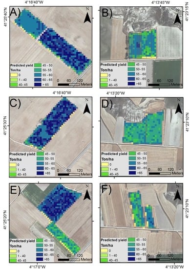
We used the svmRadial_3 model to generate the predicted yield maps of the studied potato fields across 2016, 2017 and 2018 on a pixel basis (Figure 4). According to Table 2, this model obtained the highest performance in terms of R2 (0.93). These maps showed a variation in yields across fields as represented by the eight classes. In general, the predicted yield per pixel ranged from 43 to 80 Ton/ha, with mean values around 59 Ton/ha. It can be observed that the low-yield class (0 Ton/ha) was mainly distributed across some field boundaries given the influence of other crop types or roads in the pixel reflectance.
Finally, we made a pre-harvest prediction of potato yield using only feature variables corresponding to July and August. The best trade-off in terms of RMSE and R2 was obtained by the random forest algorithm with different pre-processing: rf_3 (RMSE = 8.751 ton/ha, R2 = 0.84 and MAE = 7.399 ton/ha), rf_4 (RMSE = 8.765 ton/ha, R2 = 0.83 and MAE = 7.046 ton/ha) and rf_2 (RMSE = 8.916 ton/ha, R2 = 0.84 and MAE = 6.717 ton/ha). The latter models were fitted with 80 % of the original dataset using k-fold cross-validation (k = 10), and then evaluated against the remaining 20 % holdout dataset. In this case, the pre-processing options applied displayed minimal influence across these three model results, such that we selected rf_3 due to its having shown the lowest RMSE score during the selection process. In addition, the number of variables selected in each scenario proved to be critical (Figure 5). In general, predicted results were less close to actual yields compared to those involving September data (Table 2). Nevertheless, rf_3 offered promising results in scenario B with RMSE = 6.470 ton/ha (11.16% RMSE), MAE = 5.052 ton/ha (8.71% MAE) and R2 = 0.89. Scenarios A and C provided quite similar scores, whereas scenario D was the worst performing one. Therefore, the best choice to predict potato yield prior to harvest was the random forest with “center” pre-processing (rf_3) and the “mtry” hyper-parameter = 5.
In order to graphically display the fitness of our methodology using only variables from July and August, we represented the actual and modelled yields.
4. Discussion
Crop yield prediction is of major importance in global and local markets as it enables early decision-making, improves agricultural commodity practices and allows market prices to be modelled [78,79]. In this work, we first evaluated ten different machine learning algorithms with different pre-processing options to compare model performances in potato crops. These results highlight the advantages of pre-processing methods such as “scale” and “center” when the ranges of values or magnitudes differ greatly across predictors [80]. At this initial stage, we used the cross-validation resampling method due to the limited number of observations [81]. In general, linear regression algorithms (rqlasso, LeapBack) obtained better results than non-linear ones (svmRadial or random forest). This may explain the use of linear models for crop yield prediction in previous works [41], although crop yield differs spatially and temporally with non-linear behaviour [82]. Nevertheless, non-linear models such as svmRadial also obtained satisfactory results in terms of R2 (0.85) and RMSE (8.949 ton/ha). We agree with other authors [83,84] that crop yield prediction requires testing both linear and non-linear approaches, since model predictive ability depends upon sample number and data quality.
Second, we selected the best performing models (rqlasso_2, LeapBack_2-3 and svmRadial_3) and compared their scores against various scenarios. It was found that removing all the predictors whose correlation coefficient was > 0.50 improved the model performance for rqlasso and LeapBack in terms of RMSE. In contrast, svmRadial in scenarios C and D outperformed its results in scenarios A and B, demonstrating its improvement when more predictors are included in this model. All of these models were evaluated against a hold-out dataset, which was not included in the train-test phase in order to avoid overfitting in the model [85,86]. Since the rqlasso and LeapBack algorithms can inherently perform feature selection methods identifying the best model that contains a given number of predictors [87], we also evaluated the models without any kind of feature selection (Table 2, Scenario D). These results showed very good performance for svmRadial_3 in terms of R2 = 0.93, MAE = 5.012 ton/ha (8.64% MAE) and RMSE = 6.781 ton/ha (11.70% RMSE). The rqlasso_2 and LeapBack_2 models performed more poorly as the number of predictors increased. Based on the results presented, we suggest the use of correlation coefficients to remove collinearity among variables when using rqlasso and LeapBack. Although these models have inherent methods to automatically reduce variables, they performed worse when the number of predictors was larger and no prior feature selection was applied. These algorithms tend to select a useful set of predictors depending on the penalty term they use, but not necessarily the most important variables to explain our data [88]. In contrast, svmRadial_3 performed better when the number of predictors was larger (scenario D), which concurs with the results obtained by Joachims [89]. Although in this case, this model may not be suitable for potato yield estimation/prediction since the multi-collinearity is not addressed properly. According to Joachims [89], support vector machine models use overfitting protection that can be tuned through the regularisation parameter C. This is a penalty parameter of the error term that determines the trade-off between smooth decision boundary and classifying the training points correctly. Although some works describe the benefits of applying feature selection procedures to improve predictive performance [90,91], we did not observe it for svmRadial_3. This may be explained by the sample size of the dataset, as suggested by Jain and Zongker [92], or by the inner regularization parameters that support-vector machine algorithms have [89]. Typically, prediction errors around 10-15 % RMSE are found in crop yield prediction literature [76,93,94]. Focusing more specifically on potato crop modelling, Hartz and Moore [95] tested a multiple linear model based on temperature and insolation in the laboratory with an accuracy of R2 = 0.93. Bala and Islam [40] used vegetation indices derived from TERRA satellite imagery to predict potato yield, and obtained the following correlation coefficients (R2): 0.84 (NDVI), 0.72 (LAI) and 0.80 (fPAR—the fraction of photosynthetically active radiation). More recent approaches, such as Al-Gaadi et al. [41], predicted potato yield using Sentinel 2 and Landsat 8 satellites, and obtained R2 values between 0.39 and 0.65. Some of our fitted models outperform previous approaches based on satellite imagery for predicting potato yield, such as svmRadial_3 (R2 = 0.93 and RMSE = 6.781 ton/ha).
Pre-harvest results emphasized the need to build several machine learning models with different pre-processing and feature selection methods to optimize model results. The rf_3 performed very well under scenario B: R2 = 0.89, RMSE = 6.470 ton/ha (11.16 % RMSE) and MAE = 5.052 ton/ha (8.71% MAE). Nevertheless, some extreme events or abnormal crop conditions in September such as diseases, pest outbreaks or water stress, can influence modelled yields causing yield overestimation, as already stated by other authors [76]. To the best of our knowledge, no one has yet attempted to make pre-harvest predictions in potato crops using satellite data. In addition, there is a demand for crop modelling tools which are able to offer a better knowledge of crop productivity. These techniques can help to alleviate extreme weather-related events that trigger food insecurity since such events may reduce food supply and the incomes of households working in the agricultural sector, particularly in food insecure regions [96].
Table S5 shows the variable importance for the rqlasso_2 (July, August and September variables) and rf_3 models (July and August variables) under scenario B. The most important variables were Band8_July, Band6_Sept, LCC_Sept, LCC_July and LCC_Aug for rqlasso_2; while Band5_Aug and LCC_Aug were the most informative for rf_3. In both models, the LCC index proved to be key given its capacity to retrieve an approximation of the chlorophyll content at leaf level. As a result, it provides information about photosynthetic capacity and plant functioning [97]. Band5_Aug and Band6_Sept also had high scores given these spectral bands’ sensitivity to chlorophyll in the red-edge, which shows them to be convenient proxies for operationally estimating biophysical parameters from Sentinel-2 [98]. Band8_July achieved the highest score of influence in rqlasso_2. Near-infrared leaf reflectance is not affected by changes in chlorophyll content, with very low leaf absorption and transmittance reaching maximum values [99]. Nevertheless, near-infrared reflectance values can detect significant differences between healthy and diseased potato plants [100]. We did not find any clear evidence to attest which month was more informative, either in the rqlasso_2 or in the rf_3.
This study confirms the feasibility of our machine learning models based on Sentinel 2 imagery and how it outperforms previous efforts in potato yield prediction. We have developed a step-wise methodology to find and build the best performing models for our study region over a three-year period. The proposed Sentinel 2 bands and indices can be used effectively to model potato crops for predicting yields in the study area, and the method can be extended to other sites in Castilla y Leon that have a similar phenological cycle for the potato. The use of this methodology in other parts of the world would require a deep understanding of tuberization and senescence dates in order to adequately build and fit the proposed models.
5. Conclusions
This study has shown the possibility of predicting potato yields using Sentinel 2 imagery and machine learning techniques for three different growing years. The use of Sentinel 2 imagery provides high spatial and temporal resolutions when compared to previous approaches, and our fitted machine learning models have proved their usefulness for modelling potato yield. In general, pre-processing techniques, such as “centering” and “scaling”, improved the model results, while the impact of feature selection methods differed depending on the algorithms. Regression quantile lasso (rqLasso: 11.67% RMSE, R2 = 0.88 and 9.18% MAE) and Leap Backwards (LeapBack: 10.94% RMSE, R2 = 0.89 and 8.95% MAE) performed better when highly correlated predictors (correlation coefficient > 0.5) were removed from the dataset. In contrast, the support vector machine radial obtained higher scores when feature selection methods were not applied at all (svmRadial: R2 = 0.93, 8.64% MAE and 11.7% RMSE). In addition, we developed a model to predict potato yield prior to harvest using the rf_3 model (R2 = 0.84, 13.55% RMSE and 10.31% MAE). The latter method evidences greater uncertainty, given the possible occurrence of certain extreme events or abnormal crop conditions in September such as diseases, pest outbreaks or water stress that cannot be included in the model and would overestimate crop yields.
The study results improve the current state of the art for potato yield modelling using satellite imagery at very high spatial and temporal resolution. More robust results may be obtained by using a larger number of samples in the original dataset. In addition, cloud cover remains an obstacle in passive remote sensing, and entails the loss of information for some areas and days. Future attempts should aim to increase the number of samples, widen the geographical area and extend the number of years studied so that models have better generalization capacity.
Supplementary Materials
The following are available online at https://www.mdpi.com/2072-4292/11/15/1745/s1. Table S1: list of survey fields with total yield (ton), area (ha), yield per area (ton.FM/ha), harvesting and sowing dates; Table S2: list of satellite images downloaded for July, August, and September from 2016 to 2018; Table S3: formulations used to obtain vegetation indices: Anthocyanin Reflectance Index, Carotenoid Reflectance Index, Inverted Red-Edge Chlorophyll Index, Leaf Chlorophyll Content, Normalized Difference Vegetation Index, Plant Senescence Reflectance Index and Weighted Difference Vegetation Index; Table S4: selected predictor variables included in each scenario; Table S5: variable importance for the rqlasso_2 (July, August and September variables) and rf_3 models (July and August variables) under scenario B. All measures of importance are scaled to have a maximum value of 100, such that the highest scores represent the most important variables in the model.
Author Contributions
Conceptualization, D.G.; Methodology, D.G., P.S.; Formal Analysis, D.G.; Validation, D.G. and P.S.; Data Curation, D.G., J.S. and J.L.C., Writing—Original Draft Preparation, D.G., Writing—Review & Editing, D.G., P.S., J.L.C., J.S.; Supervision, J.S. and J.L.C.; Project Administration, J.S.
Funding
This research did not receive any specific grant from funding agencies in the public, commercial, or not-for-profit sectors.
Acknowledgments
Crop yield production was facilitated by the potato grower, to whom we are grateful for his cooperation in this research. In addition, we thank the anonymous reviewers for their constructive comments, which have helped us enormously to improve the manuscript and to render its final form.
Conflicts of Interest
All authors declare that they have no conflict of interest.
References
- Seelan, S.K.; Laguette, S.; Casady, G.M.; Seielstad, G.A. Remote sensing applications for precision agriculture: A learning community approach. Remote Sens. Environ. 2003, 88, 157–169. [Google Scholar] [CrossRef]
- Lotze-Campen, H.; Müller, C.; Bondeau, A.; Rost, S.; Popp, A.; Lucht, W. Global food demand, productivity growth, and the scarcity of land and water resources: A spatially explicit mathematical programming approach. Agric. Econ. 2008, 39, 325–338. [Google Scholar] [CrossRef]
- Rijsberman, F.R.; Molden, D. Balancing water uses: Water for food and water for nature. In Thematic Background Paper, Proceedings of the International Conference on Freshwater, Bonn, Germany, 3–7 December 2001; IWRA: Paris, France, 2001; Available online: https://cdn.atria.nl/epublications/2001/Balancing_water_uses.pdf (accessed on 15 April 2019).
- Nelson, G.C.; Valin, H.; Sands, R.D.; Havlík, P.; Ahammad, H.; Deryng, D.; Kyle, P. Climate change effects on agriculture: Economic responses to biophysical shocks. Proc. Natl. Acad. Sci. USA 2014, 111, 3274–3279. [Google Scholar] [CrossRef] [PubMed]
- Bindraban, P.S.; van der Velde, M.; Ye, L.; Van den Berg, M.; Materechera, S.; Kiba, D.I.; Hoogmoed, W. Assessing the impact of soil degradation on food production. Curr. Opin. Environ. Sustain. 2012, 4, 478–488. [Google Scholar] [CrossRef]
- Conijn, J.G.; Bindraban, P.S.; Schröder, J.J.; Jongschaap, R.E.E. Can our global food system meet food demand within planetary boundaries? Agric. Ecosyst. Environ. 2018, 251, 244–256. [Google Scholar] [CrossRef]
- Windfuhr, M.; Jonsén, J. Food Sovereignty: Towards Democracy in Localized Food Systems. 2005. Available online: http://agris.fao.org/agris-search/search.do?recordID=GB2013202621 (accessed on 15 April 2019).
- Doran, J.W. Soil health and global sustainability: Translating science into practice. Agric. Ecosyst. Environ. 2002, 88, 119–127. [Google Scholar] [CrossRef]
- Fischer, G.; Shah, M.; Tubiello, F.N.; Van Velhuizen, H. Socio-economic and climate change impacts on agriculture: An integrated assessment, 1990–2080. Philos. Trans. R. Soc. Lond. B Biol. Sci. 2005, 360, 2067–2083. [Google Scholar] [CrossRef] [PubMed]
- Zarco-Tejada, P.; Hubbard, N.; Loudjani, P. Precision Agriculture: An Opportunity for EU Farmers—Potential Support with the CAP 2014–2020. Jt. Res. Cent. (JRC) Eur. Comm. 2014. Available online: http://www.europarl.europa.eu/RegData/etudes/note/join/2014/529049/IPOL-AGRI_NT%282014%29529049_EN.pdf (accessed on 15 April 2019).
- Gebbers, R.; Adamchuk, V.I. Precision agriculture and food security. Science 2010, 327, 828–831. [Google Scholar] [CrossRef]
- Chen, F.; Kissel, D.E.; West, L.T.; Adkins, W. Field-scale mapping of surface soil organic carbon using remotely sensed imagery. Soil Sci. Soc. Am. J. 2000, 64, 746–753. [Google Scholar] [CrossRef]
- Wardlow, B.D.; Egbert, S.L.; Kastens, J.H. Analysis of time-series MODIS 250 m vegetation index data for crop classification in the US Central Great Plains. Remote Sens. Environ. 2007, 108, 290–310. [Google Scholar] [CrossRef]
- Singh, R.K.; Budde, M.E.; Senay, G.B.; Rowland, J. A Novel Approach for Forecasting Crop Production and Yield Using Remotely Sensed Satellite Images. In AGU Fall Meeting Abstracts, 2017. Available online: http://adsabs.harvard.edu/abs/2017AGUFMIN54A..03S (accessed on 12 February 2019).
- Shakoor, N.; Lee, S.; Mockler, T.C. High throughput phenotyping to accelerate crop breeding and monitoring of diseases in the field. Curr. Opin. Plant Biol. 2017, 38, 184–192. [Google Scholar] [CrossRef] [PubMed]
- Mohanty, B.P.; Cosh, M.H.; Lakshmi, V.; Montzka, C. Soil moisture remote sensing: State-of-the-science. Vadose Zone J. 2017, 16, 1. [Google Scholar] [CrossRef]
- Sharma, L.K.; Bali, S.K.; Dwyer, J.D.; Plant, A.B.; Bhowmik, A. A case study of improving yield prediction and sulfur deficiency detection using optical sensors and relationship of historical potato yield with weather data in Maine. Sensors 2017, 17, 1095. [Google Scholar] [CrossRef] [PubMed]
- Huang, Y.; Chen, Z.X.; Tao, Y.U.; Huang, X.Z.; Gu, X.F. Agricultural remote sensing big data: Management and applications. J. Integr. Agric. 2018, 17, 1915–1931. [Google Scholar] [CrossRef]
- Wolfert, S.; Ge, L.; Verdouw, C.; Bogaardt, M.J. Big data in smart farming—A review. Agric. Syst. 2017, 153, 69–80. [Google Scholar] [CrossRef]
- Zhang, D. Advances in machine learning applications in software engineering. Igi Glob. 2006. [Google Scholar] [CrossRef]
- Chlingaryan, A.; Sukkarieh, S.; Whelan, B. Machine learning approaches for crop yield prediction and nitrogen status estimation in precision agriculture: A review. Comput. Electron. Agric. 2018, 151, 61–69. [Google Scholar] [CrossRef]
- Dahikar, S.S.; Rode, S.V. Agricultural crop yield prediction using artificial neural network approach. Int. J. Innov. Res. Electr. Electron. Instrum. Control Eng. 2014, 2, 683–686. Available online: https://pdfs.semanticscholar.org/7c68/a32212c1f86f535f4c1658ff68399d0a9ddd.pdf (accessed on 15 April 2019).
- Pantazi, X.E.; Moshou, D.; Alexandridis, T.; Whetton, R.L.; Mouazen, A.M. Wheat yield prediction using machine learning and advanced sensing techniques. Comput. Electron. Agric. 2016, 121, 57–65. [Google Scholar] [CrossRef]
- Veenadhari, S.; Misra, B.; Singh, C.D. Machine learning approach for forecasting crop yield based on climatic parameters. In Proceedings of the International Conference on IEEE Computer Communication and Informatics (ICCCI), Coimbatore, Tamilnadu, 3–5 January 2014; pp. 1–5. [Google Scholar] [CrossRef]
- Raymundo, R.; Asseng, S.; Robertson, R.; Petsakos, A.; Hoogenboom, G.; Quiroz, R.; Wolf, J. Climate change impact on global potato production. Eur. J. Agron. 2018, 100, 87–98. [Google Scholar] [CrossRef]
- Devaux, A.; Kromann, P.; Ortiz, O. Potatoes for sustainable global food security. Potato Res. 2014, 57, 185–199. [Google Scholar] [CrossRef]
- Bowen, W.; Cabrera, H.; Barrera, V.H.; Baigorria, G. Simulating the Response of Potato to Applied Nitrogen. CIP Program Report 1997–1998. 1999; pp. 381–386. Available online: http://repositorio.iniap.gob.ec/handle/41000/2784 (accessed on 29 May 2019).
- Molahlehi, L.; Steyn, J.M.; Haverkort, A.J. Potato crop response to genotype and environment in a subtropical highland agro-ecology. Potato Res. 2013, 56, 237–258. [Google Scholar] [CrossRef]
- Machakaire, A.T.; Steyn, J.M.; Caldiz, D.O.; Haverkort, A.J. Forecasting yield and tuber size of processing potatoes in South Africa using the LINTUL-potato-DSS model. Potato Res. 2016, 59, 195–206. [Google Scholar] [CrossRef]
- Bélanger, G.; Walsh, J.R.; Richards, J.E.; Milburn, P.H.; Ziadi, N. Comparison of three statistical models describing potato yield response to nitrogen fertilizer. Agron. J. 2000, 92, 902–908. [Google Scholar] [CrossRef]
- Kooman, P.L.; Haverkort, A.J. Modelling development and growth of the potato crop influenced by temperature and daylength: LINTUL-POTATO. In Potato Ecology and Modelling of Crops under Conditions Limiting Growth; Springer: Dordrecht, The Netherlands, 1995; pp. 41–59. [Google Scholar] [Green Version]
- Manrique, L.A.; Kinry, J.R.; Hodges, T.; Axness, D.S. Dry matter production and radiation interception of potato. Crop Sci. 1991, 31, 1044–1049. [Google Scholar] [CrossRef]
- Fleisher, D.H.; Condori, B.; Quiroz, R.; Alva, A.; Asseng, S.; Barreda, C.; Bindi, M.; Boote, K.J.; Ferrise, R.; Franke, A.C. A potato model intercomparison across varying climates and productivity levels. Glob. Chang. Biol. 2017, 23, 1258–1281. [Google Scholar] [CrossRef] [PubMed]
- Raymundo, R.; Asseng, S.; Cammarano, D.; Quiroz, R. Potato, sweet potato, and yam models for climate change: A review. Field Crop. Res. 2014, 166, 173–185. [Google Scholar] [CrossRef]
- Saue, T.; Kadaja, J. Water limitations on potato yield in Estonia assessed by crop modelling. Agric. For. Meteorol. 2014, 194, 20–28. [Google Scholar] [CrossRef]
- Borus, D.; Parsons, D.; Boersma, M.; Brown, H.; Mohammed, C. Improving the prediction of potato productivity: APSIM-Potato model parameterization and evaluation in Tasmania, Australia. Aust. J. Crop Sci. 2018, 12, 32. [Google Scholar] [CrossRef]
- Basu, S.K.; Kumar, N. Modelling and Simulation of Diffusive Processes; Springer International: Basel, Switzerlan, 2016. [Google Scholar]
- Awad, M.M. Toward Precision in Crop Yield Estimation Using Remote Sensing and Optimization Techniques. Agriculture 2019, 9, 54. [Google Scholar] [CrossRef]
- Hoefsloot, P.; Ines, A.V.; Dam, J.C.V.; Duveiller, G.; Kayitakire, F.; Hansen, J. Combining crop models and remote sensing for yield prediction: Concepts, applications and challenges for heterogeneous smallholder environments. In Proceedings of the Report of CCFAS-JRC Workshop at Joint Research Centre, Ispra, Italy, 13–14 June 2012; Joint Research Center Technical Report. Publications Office of the European Union: Luxembourg, 2012. Available online: http://publications.jrc.ec.europa.eu/repository/bitstream/JRC77375/lbna25643enn.pdf (accessed on 29 May 2019).
- Bala, S.K.; Islam, A.S. Correlation between potato yield and MODIS-derived vegetation indices. Int. J. Remote Sens. 2009, 30, 2491–2507. [Google Scholar] [CrossRef]
- Al-Gaadi, K.A.; Hassaballa, A.A.; Tola, E.; Kayad, A.G.; Madugundu, R.; Alblewi, B.; Assiri, F. Prediction of potato crop yield using precision agriculture techniques. PLoS ONE 2016, 11, e0162219. [Google Scholar] [CrossRef] [PubMed]
- Clevers, J.G.; Gitelson, A.A. Remote estimation of crop and grass chlorophyll and nitrogen content using red-edge bands on Sentinel-2 and-3. Int. J. Appl. Earth Obs. Geoinf. 2013, 23, 344–351. [Google Scholar] [CrossRef]
- Zheng, T.; Liu, N.; Wu, L.; Li, M.; Sun, H.; Zhang, Q.; Wu, J. Estimation of Chlorophyll Content in Potato Leaves Based on Spectral Red Edge Position. IFAC-PapersOnLine 2018, 51, 602–606. [Google Scholar] [CrossRef]
- Jongschaap, R.E.; Booij, R. Spectral measurements at different spatial scales in potato: Relating leaf, plant and canopy nitrogen status. Int. J. Appl. Earth Obs. Geoinf. 2004, 5, 205–218. [Google Scholar] [CrossRef]
- European Space Agency—ESA. Mission Sentinel 2, Overview. 2016. Available online: https://sentinel.esa.int/web/sentinel/missions/sentinel-2 (accessed on 4 May 2019).
- Statista. 2017. Available online: https://es.statista.com/estadisticas/510906/produccion-de-patatas-en-espana-por-comunidad-autonoma/ (accessed on 2 May 2019).
- JCyL—Junta de Castilla y Leon. 2015. Available online: http://www.jcyl.es/web/jcyl/AgriculturaGanaderia/es/Plantilla100Detalle/1246464862173/_/1284142623007/Comunicacion?plantillaObligatoria=PlantillaContenidoNoticiaHome (accessed on 31 October 2018).
- Kottek, M.; Grieser, J.; Beck, C.; Rudolf, B.; Rubel, F. World map of the Köppen-Geiger climate classification updated. Meteorol. Z. 2006, 15, 259–263. [Google Scholar] [CrossRef]
- JCyL—Junta de Castilla y Leon. 2018. Available online: http://datosabiertos.jcyl.es/web/jcyl/set/es/cartografia/SIGPAC/1284225645888 (accessed on 15 August 2018).
- ESRI. ArcGIS Desktop: Release 10.4; Environmental Systems Research Institute: Redlands, CA, USA, 2014. [Google Scholar]
- Louis, J.; Debaecker, V.; Pflug, B.; Main-Korn, M.; Bieniarz, J.; Mueller-Wilm, U.; Gascon, F. Sentinel-2 Sen2Cor: L2A Processor for Users. Living Planet Symp. 2016, 740, 91. Available online: https://elib.dlr.de/107381/1/LPS2016_sm10_3louis.pdf (accessed on 15 April 2019).
- Hijmans, R.J.; van Etten, J. Raster: Geographic data analysis and modeling. R Pack. Vers. 2014, 2, 8. Available online: https://rdrr.io/cran/raster/f/inst/doc/rasterfile.pdf (accessed on 24 June 2019).
- R Core Team. R: A Language and Environment for Statistical Computing; R Foundation for Statistical Computing: Vienna, Austria, 2017; Available online: https://www.R-project.org/ (accessed on 4 May 2019).
- Gitelson, A.A.; Merzlyak, M.N.; Chivkunova, O.B. Optical properties and nondestructive estimation of anthocyanin content in plant leaves. Photochem. Photobiol. 2001, 74, 38–45. [Google Scholar] [CrossRef]
- Gitelson, A.A.; Zur, Y.; Chivkunova, O.B.; Merzlyak, M.N. Assessing Carotenoid Content in Plant Leaves with Reflectance Spectroscopy. Photochem. Photobiol. 2002, 75, 272–281. [Google Scholar] [CrossRef]
- Frampton, W.J.; Dash, J.; Watmough, G.; Milton, E.J. Evaluating the capabilities of Sentinel-2 for quantitative estimation of biophysical variables in vegetation. ISPRS J. Photogramm. Remote Sens. 2013, 82, 83–92. [Google Scholar] [CrossRef] [Green Version]
- Haboudane, D.; Miller, J.R.; Tremblay, N.; Zarco-Tejada, P.J.; Dextraze, L. Integrated narrow-band vegetation indices for prediction of crop chlorophyll content for application to precision agriculture. Remote Sens. Environ. 2002, 81, 416–426. [Google Scholar] [CrossRef]
- Rouse, J.W.; Haas, R.H.; Schell, J.A.; Deering, J.A. Monitoring vegetation systems in the Great Plains with ERTS. In Proceedings of the Third Symposium on Significant Results Obtained with ERTS-1, Washington, DC, USA, 10–14 December 1973; pp. 309–317. [Google Scholar]
- Merzlyak, M.N.; Gitelson, A.A.; Chivkunova, O.B.; Rakitin, V.Y. Non-destructive optical detection of pigment changes during leaf senescence and fruit ripening. Physiol. Plant. 1999, 106, 135–141. [Google Scholar] [CrossRef] [Green Version]
- Clevers, J.G.P.W. Application of a weighted infrared-red vegetation index for estimating leaf area index by correcting for soil moisture. Remote Sens. Environ. 1989, 29, 25–37. [Google Scholar] [CrossRef]
- Agakov, F.; Bonilla, E.; Cavazos, J.; Franke, B.; Fursin, G.; O’Boyle, M.F.; Williams, C.K. Using machine learning to focus iterative optimization. In Proceedings of the International Symposium on Code Generation and Optimization, New York, NY, USA, 26–29 March 2006; IEEE Computer Society: Washington, DC, USA, 2006; pp. 295–305. [Google Scholar]
- Nelder, J.A.; Wedderburn, R.W. Generalized linear models. J. R. Stat. Soc. Ser. A (Gen.) 1972, 135, 370–384. [Google Scholar] [CrossRef]
- Lumley, T.; Lumley, M.T. Package ‘leaps’. Regression Subset Selection. Thomas Lumley Based on Fortran Code by Alan Miller. 2017. Available online: https://cran.r-project.org/web/packages/leaps/index.html (accessed on 3 May 2019).
- Tibshirani, R. Regression shrinkage and selection via the lasso. J. R. Stat. Soc. Ser. B (Methodol.) 1996, 58, 267–288. [Google Scholar] [CrossRef]
- Cortes, C.; Vapnik, V. Support-vector networks. Mach. Learn. 1995, 20, 273–297. [Google Scholar] [CrossRef]
- Scholkopf, B.; Sung, K.K.; Burges, C.J.; Girosi, F.; Niyogi, P.; Poggio, T.; Vapnik, V. Comparing support vector machines with Gaussian kernels to radial basis function classifiers. IEEE Trans. Signal Process. 1997, 45, 2758–2765. [Google Scholar] [CrossRef]
- Breiman, L. Random forests. Mach. Learn. 2001, 45, 5–32. [Google Scholar] [CrossRef]
- Friedman, J.H. Multivariate Adaptive Regression Splines. Ann. Stat. 1991, 19, 1–67. [Google Scholar] [CrossRef]
- Hechenbichler, K.; Schliep, K. Weighted k-nearest-neighbor techniques and ordinal classification. LMU 2004. [CrossRef]
- Burton, T.A. Averaged neural networks. Neural Netw. 1993, 6, 677–680. [Google Scholar] [CrossRef]
- Kuhn, M. Caret package. J. Stat. Softw. 2008, 28, 1–26. Available online: http://www.math.chalmers.se/Stat/Grundutb/GU/MSA220/S18/caret-JSS.pdf (accessed on 15 April 2019).
- Kuhn, M.; Weston, S.; Keefer, C.; Coulter, N.; Quinlan, R. Cubist: Rule-and Instance-Based Regression Modeling. R Package Version 0.0. 15. 2013. Available online: http://www2.uaem.mx/r-mirror/web/packages/Cubist/Cubist.pdf (accessed on 15 April 2019).
- Brownlee, J. Feature Selection with the Caret R Package. 2014. Available online: https://machinelearningmastery.com/feature-selection-with-the-caret-r-package/ (accessed on 2 November 2018).
- Perez-Riverol, Y.; Kuhn, M.; Vizcaíno, J.A.; Hitz, M.P.; Audain, E. Accurate and fast feature selection workflow for high-dimensional omics data. PLoS ONE 2017, 12, e0189875. [Google Scholar] [CrossRef] [PubMed]
- Brownlee, J. A Gentle Introduction to k-Fold Cross-Validation. 2018. Available online: https://machinelearningmastery.com/k-fold-cross-validation/ (accessed on 2 November 2018).
- Mkhabela, M.S.; Bullock, P.; Raj, S.; Wang, S.; Yang, Y. Crop yield forecasting on the Canadian Prairies using MODIS NDVI data. Agric. For. Meteorol. 2011, 151, 385–393. [Google Scholar] [CrossRef]
- Akhand, K.; Nizamuddin, M.; Roytman, L.; Kogan, F. Using remote sensing satellite data and artificial neural network for prediction of potato yield in Bangladesh. Int. Soc. Opt. Photon. 2016, 9975, 997508. [Google Scholar] [CrossRef]
- Idso, S.B.; Reginato, R.J.; Hatfield, J.L.; Walker, G.K.; Jackson, R.D.; Pinter, P.J., Jr. A generalization of the stress-degree-day concept of yield prediction to accommodate a diversity of crops. Agric. Meteorol. 1980, 21, 205–211. [Google Scholar] [CrossRef]
- Peng, Y.H.; Hsu, C.S.; Huang, P.C. Developing crop price forecasting service using open data from Taiwan markets. In Proceedings of the 2015 Conference on Technologies and Applications of Artificial Intelligence (TAAI), Tainan, Taiwan, 20–22 November 2015; pp. 172–175. [Google Scholar] [CrossRef]
- Guyon, I.; Elisseeff, A. An introduction to variable and feature selection. J. Mach. Learn. Res. 2003, 3, 1157–1182. Available online: http://www.jmlr.org/papers/volume3/guyon03a/guyon03a.pdf (accessed on 15 April 2019).
- Picard, R.R.; Cook, R.D. Cross-validation of regression models. J. Am. Stat. Assoc. 1984, 79, 575–583. [Google Scholar] [CrossRef]
- Drummond, S.T.; Sudduth, K.A.; Joshi, A.; Birrell, S.J.; Kitchen, N.R. Statistical and neural methods for site–specific yield prediction. Trans. ASAE 2003, 46, 5. [Google Scholar] [CrossRef]
- Li, A.; Liang, S.; Wang, A.; Qin, J. Estimating crop yield from multi-temporal satellite data using multivariate regression and neural network techniques. Photogramm. Eng. Remote Sens. 2007, 73, 1149–1157. [Google Scholar] [CrossRef]
- Sayago, S.; Bocco, M. Crop yield estimation using satellite images: Comparison of linear and non-linear models. AgriScientia 2018, 1, 1–9. [Google Scholar] [CrossRef]
- Hawkins, D.M. The problem of overfitting. J. Chem. Inf. Comput. Sci. 2004, 44, 1–12. [Google Scholar] [CrossRef] [PubMed]
- Perrone, M.P.; Cooper, L.N. When networks disagree: Ensemble methods for hybrid neural networks (No. TR-61). Brown Univ. Provid. Ri Inst. Brain Neural Syst. 1992. Available online: https://apps.dtic.mil/dtic/tr/fulltext/u2/a260121.pdf (accessed on 15 April 2019).
- James, G.; Witten, D.; Hastie, T.; Tibshirani, R. An Introduction to Statistical Learning; Springer: Berlin/Heidelberg, Germany, 2013; p. 112. [Google Scholar]
- Friedman, J.; Hastie, T.; Tibshirani, R. The Elements of Statistical Learning; Springer: Berlin/Heidelberg, Germany, 2001. [Google Scholar]
- Joachims, T. Text categorization with support vector machines: Learning with many relevant features. In Proceedings of the European conference on machine learning, Vienna, Austria, 12–14 July 1982; Springer: Berlin/Heidelberg, Germany, 1982; pp. 137–142. [Google Scholar] [CrossRef]
- Blum, A.L.; Langley, P. Selection of relevant features and examples in machine learning. Artif. Intell. 1997, 97, 245–271. [Google Scholar] [CrossRef] [Green Version]
- Guyon, I.; Weston, J.; Barnhill, S.; Vapnik, V. Gene selection for cancer classification using support vector machines. Mach. Learn. 2002, 46, 389–422. [Google Scholar] [CrossRef]
- Jain, A.; Zongker, D. Feature selection: Evaluation, application, and small sample performance. IEEE Trans. Pattern Anal. Mach. Intell. 1997, 19, 153–158. [Google Scholar] [CrossRef]
- Baez-Gonzalez, A.D.; Kiniry, J.R.; Maas, S.J.; Tiscareno, M.L.; Macias, C.J.J.L.; Mendoza, J.L.; Manjarrez, J.R. Large-area maize yield forecasting using leaf area index based yield model. Agron. J. 2005, 97, 418–425. [Google Scholar] [CrossRef]
- Launay, M.; Guerif, M. Assimilating remote sensing data into a crop model to improve predictive performance for spatial applications. Agric. Ecosyst. Environ. 2005, 111, 321–339. [Google Scholar] [CrossRef]
- Hartz, T.K.; Moore, F.D. Prediction of potato yield using temperature and insolation data. Am. Potato J. 1978, 55, 431–436. [Google Scholar] [CrossRef]
- Brown, M.E. Satellite remote sensing in agriculture and food security assessment. Procedia Environ. Sci. 2015, 29, 307. [Google Scholar] [CrossRef]
- Kooistra, L.; Clevers, J.G. Estimating potato leaf chlorophyll content using ratio vegetation indices. Remote Sens. Lett. 2016, 7, 611–620. [Google Scholar] [CrossRef] [Green Version]
- Delegido, J.; Verrelst, J.; Alonso, L.; Moreno, J. Evaluation of sentinel-2 red-edge bands for empirical estimation of green LAI and chlorophyll content. Sensors 2011, 11, 7063–7081. [Google Scholar] [CrossRef] [PubMed]
- Gogoi, N.K.; Deka, B.; Bora, L.C. Remote sensing and its use in detection and monitoring plant diseases: A review. Agric. Rev. 2018, 39, 4. [Google Scholar] [CrossRef]
- Duarte-Carvajalino, J.; Alzate, D.; Ramirez, A.; Santa-Sepulveda, J.; Fajardo-Rojas, A.; Soto-Suárez, M. Evaluating Late Blight Severity in Potato Crops Using Unmanned Aerial Vehicles and Machine Learning Algorithms. Remote Sens. 2018, 10, 1513. [Google Scholar] [CrossRef]
Figure 1.
Location of the study fields (pink colour) in the municipality of Cuellar (in red colour), Castilla y León (Spain).
Figure 1.
Location of the study fields (pink colour) in the municipality of Cuellar (in red colour), Castilla y León (Spain).

Figure 2.
Performance of rqlasso_2, LeapBack_2, LeapBack_3 and svmRadial_3 models in terms of RSME, MAE and R2 for scenario B.
Figure 2.
Performance of rqlasso_2, LeapBack_2, LeapBack_3 and svmRadial_3 models in terms of RSME, MAE and R2 for scenario B.

Figure 3.
Comparison between predicted and actual yields using (a) rqlasso_2 (scenario B), (b) LeapBack_2 (scenario B), and (c) svmRadial_3 (scenario D) with the July, August and September predictors. Graph values are the overall amount of individual predictions over ten iterations per model.
Figure 3.
Comparison between predicted and actual yields using (a) rqlasso_2 (scenario B), (b) LeapBack_2 (scenario B), and (c) svmRadial_3 (scenario D) with the July, August and September predictors. Graph values are the overall amount of individual predictions over ten iterations per model.

Figure 4.
Maps of predicted potato yield for svmRadial_3 under scenario D across the study period: (A,B) 2016, (C,D) 2017, (E,F) 2018.
Figure 4.
Maps of predicted potato yield for svmRadial_3 under scenario D across the study period: (A,B) 2016, (C,D) 2017, (E,F) 2018.

Figure 5.
Random forest model (rf_3) with “center” pre-processing across four feature selection scenarios, with July and August predictors.
Figure 5.
Random forest model (rf_3) with “center” pre-processing across four feature selection scenarios, with July and August predictors.

Figure 6.
Comparison between predicted and actual yields using the random forest model (rf_3) with July and August predictor variables under scenario B.
Figure 6.
Comparison between predicted and actual yields using the random forest model (rf_3) with July and August predictor variables under scenario B.


Table 1.
The twenty models selected based on performance, statistical analysis indices of RMSE, R2, and MAE, and the optimum tuning values that yield the smallest RMSE score.
Table 1.
The twenty models selected based on performance, statistical analysis indices of RMSE, R2, and MAE, and the optimum tuning values that yield the smallest RMSE score.
| No | Model | RMSE | R2 | MAE | Best Tuning Par. |
|---|---|---|---|---|---|
| 1 | rqlasso_2 | 7.374 | 0.84 | 6.562 | lambda = 0.0001 |
| 2 | LeapBack_3 | 8.239 | 0.89 | 6.489 | nvmax = 2 |
| 3 | LeapBack_2 | 8.278 | 0.84 | 6.617 | nvmax = 2 |
| 4 | svmRadial_3 | 8.949 | 0.85 | 7.263 | Sigma = 0.0574157 and C = 1 |
| 5 | rqlasso_1 | 9.019 | 0.78 | 7.740 | lambda = 0.1 |
| 6 | rqlasso_4 | 9.046 | 0.85 | 7.409 | lambda = 0.1 |
| 7 | LeapBack_4 | 9.050 | 0.85 | 7.402 | nvmax = 2 |
| 8 | rqlasso_3 | 9.086 | 0.81 | 7.416 | lambda = 0.1 |
| 9 | cubist_Ensemble | 9.168 | 0.38 | 6.550 | - |
| 10 | glm_1 | 9.228 | 0.77 | 7.786 | - |
| 11 | rf_3 | 9.234 | 0.84 | 7.386 | Mtry = 6 |
| 12 | svmLinear_4 | 9.577 | 0.76 | 7.967 | C = 1 |
| 13 | svmLinear_2 | 9.618 | 0.73 | 7.539 | C = 1 |
| 14 | rf_2 | 9.643 | 0.80 | 7.366 | Mtry = 6 |
| 15 | glm_3 | 9.753 | 0.82 | 7.922 | - |
| 16 | svmLinear_3 | 9.761 | 0.87 | 7.423 | C = 1 |
| 17 | rf_1 | 9.787 | 0.80 | 8.201 | Mtry = 6 |
| 18 | mars_1 | 9.813 | 0.77 | 7.824 | nprune = 2 and degree = 1 |
| 19 | kknn_4 | 9.933 | 0.75 | 8.658 | kmax = 9, distance = 2 and kernel = optimal |
| 20 | svmRadial_2 | 9.937 | 0.71 | 7.605 | Sigma = 0.0873 and C = 1 |
Table 2.
Model performance for each of the proposed scenarios (A, B, C and D) based on RMSE (ton/ha), R2, and MAE (ton/ha). Average * is the mean score value for all the models with the exception of LeapBack_3, given that model results are identical to LeapBack_2.
Table 2.
Model performance for each of the proposed scenarios (A, B, C and D) based on RMSE (ton/ha), R2, and MAE (ton/ha). Average * is the mean score value for all the models with the exception of LeapBack_3, given that model results are identical to LeapBack_2.
| Feature Selection | Corr. < 0.5 | Corr. < 0.75 | Corr. < 0.90 | No Feature Selection | ||||||||
|---|---|---|---|---|---|---|---|---|---|---|---|---|
| Scenario | A | B | C | D | ||||||||
| RMSE | R2 | MAE | RMSE | R2 | MAE | RMSE | R2 | MAE | RMSE | R2 | MAE | |
| rqlasso_2 | 6.768 | 0.88 | 5.320 | 7.093 | 0.90 | 5.653 | 8.456 | 0.89 | 6.326 | 7.844 | 0.86 | 5.730 |
| svmRadial_3 | 9.125 | 0.72 | 6.804 | 7.710 | 0.83 | 5.769 | 7.370 | 0.89 | 5.242 | 6.781 | 0.93 | 5.015 |
| LeapBack_2 | 6.341 | 0.89 | 5.192 | 6.866 | 0.89 | 5.512 | 10.455 | 0.75 | 8.502 | 8.319 | 0.81 | 6.981 |
| LeapBack_3 | 6.341 | 0.89 | 5.192 | 6.866 | 0.89 | 5.512 | 10.455 | 0.75 | 8.502 | 8.319 | 0.81 | 6.981 |
| Average * | 7.411 | 0.83 | 5.772 | 7.223 | 0.87 | 5.645 | 8.760 | 0.84 | 6.690 | 7.648 | 0.87 | 5.909 |
© 2019 by the authors. Licensee MDPI, Basel, Switzerland. This article is an open access article distributed under the terms and conditions of the Creative Commons Attribution (CC BY) license (http://creativecommons.org/licenses/by/4.0/).
Share and Cite
MDPI and ACS Style
Gómez, D.; Salvador, P.; Sanz, J.; Casanova, J.L. Potato Yield Prediction Using Machine Learning Techniques and Sentinel 2 Data. Remote Sens. 2019, 11, 1745. https://doi.org/10.3390/rs11151745
AMA Style
Gómez D, Salvador P, Sanz J, Casanova JL. Potato Yield Prediction Using Machine Learning Techniques and Sentinel 2 Data. Remote Sensing. 2019; 11(15):1745. https://doi.org/10.3390/rs11151745
Chicago/Turabian StyleGómez, Diego, Pablo Salvador, Julia Sanz, and Jose Luis Casanova. 2019. "Potato Yield Prediction Using Machine Learning Techniques and Sentinel 2 Data" Remote Sensing 11, no. 15: 1745. https://doi.org/10.3390/rs11151745
Note that from the first issue of 2016, this journal uses article numbers instead of page numbers. See further details here.