Optimal Cyanobacterial Pigment Retrieval from Ocean Colour Sensors in a Highly Turbid, Optically Complex Lake

 , ,
, ,
Abstract
:
1. Introduction
2. Materials and Methods
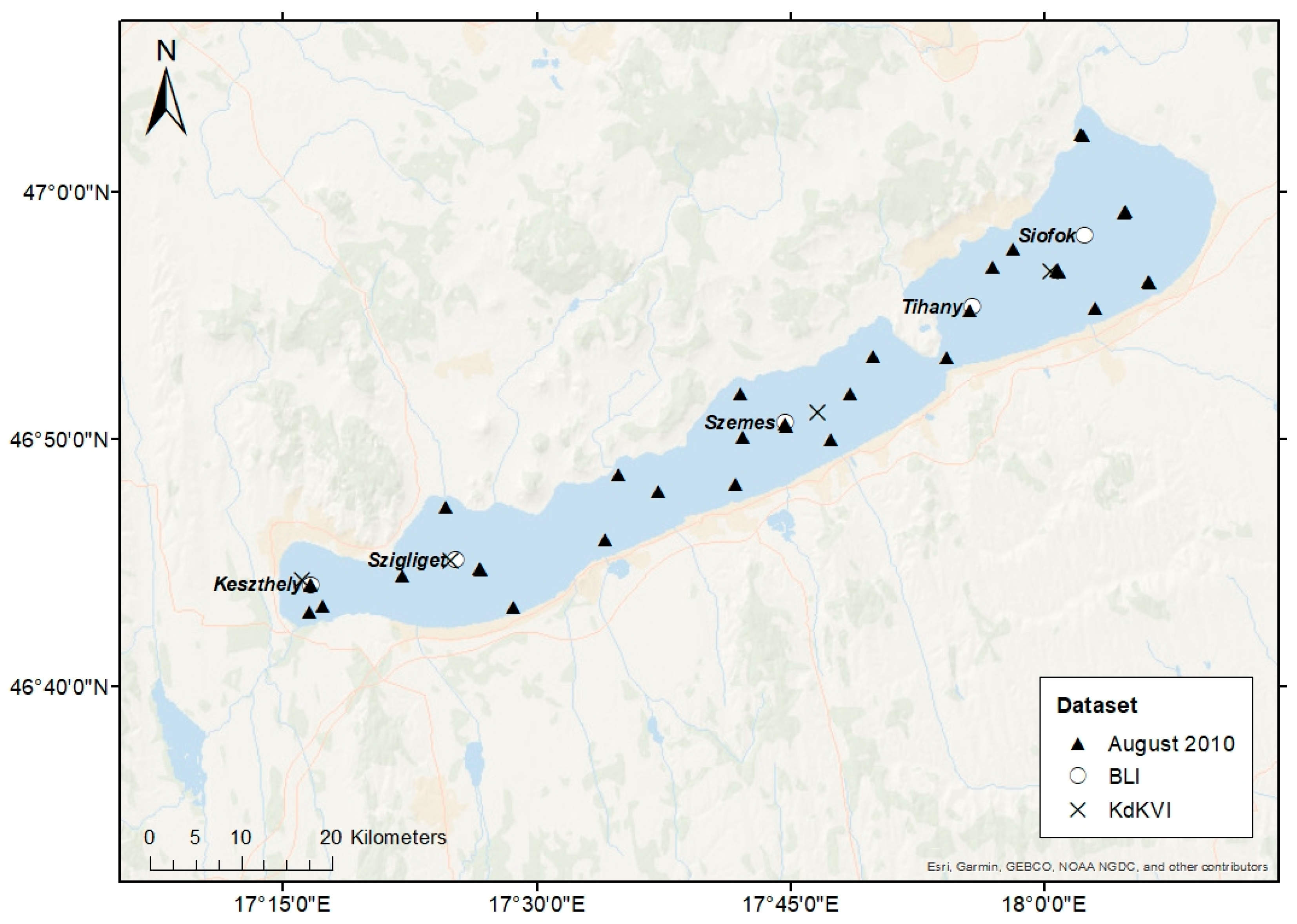
2.1. Study Site
2.2. Validation Datasets
2.2.1. Chlorophyll-a
2.2.2. Phycocyanin
2.2.3. Phytoplankton Biomass
2.2.4. Measurement of Absorption and Backscattering Coefficients
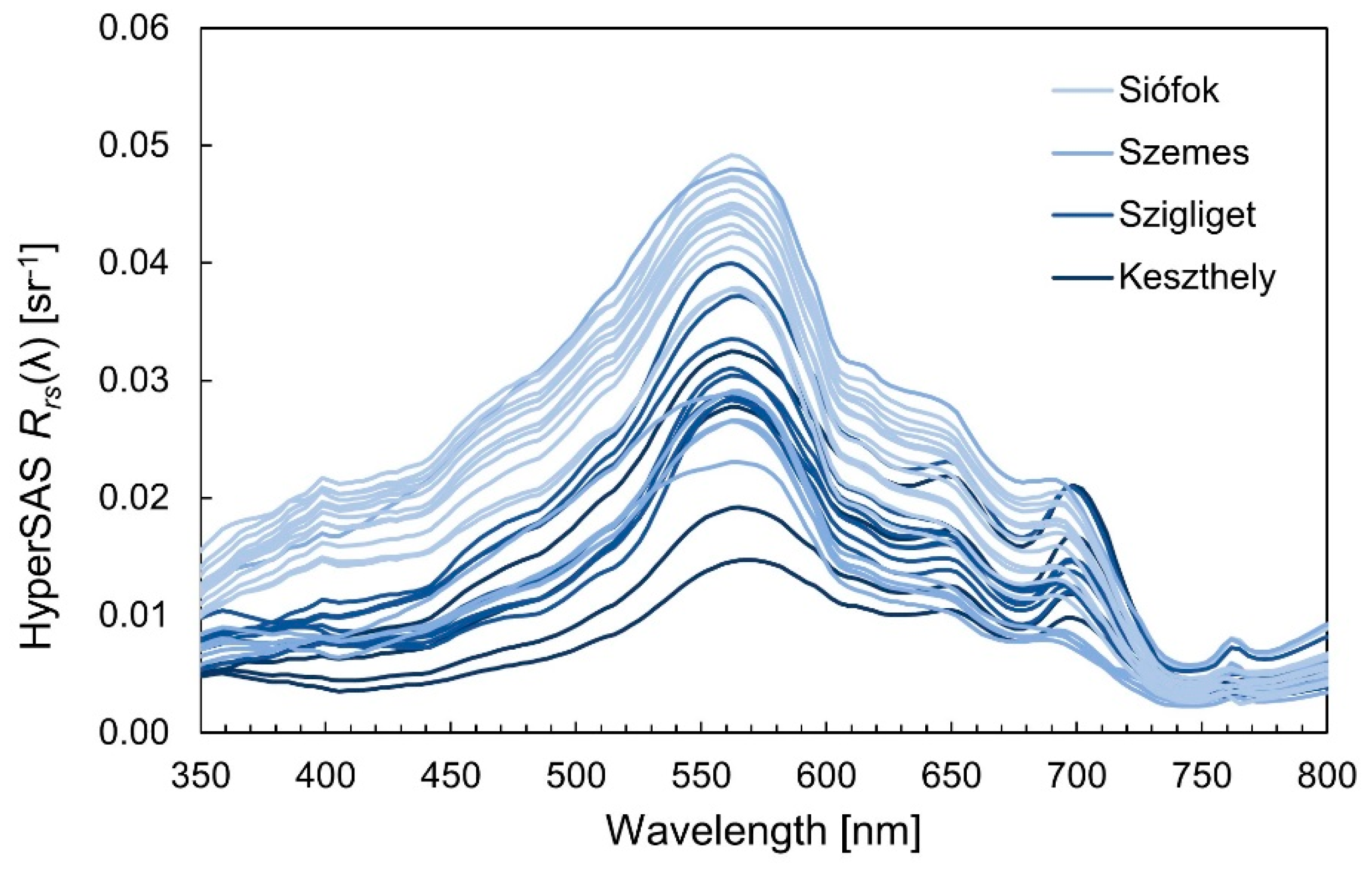
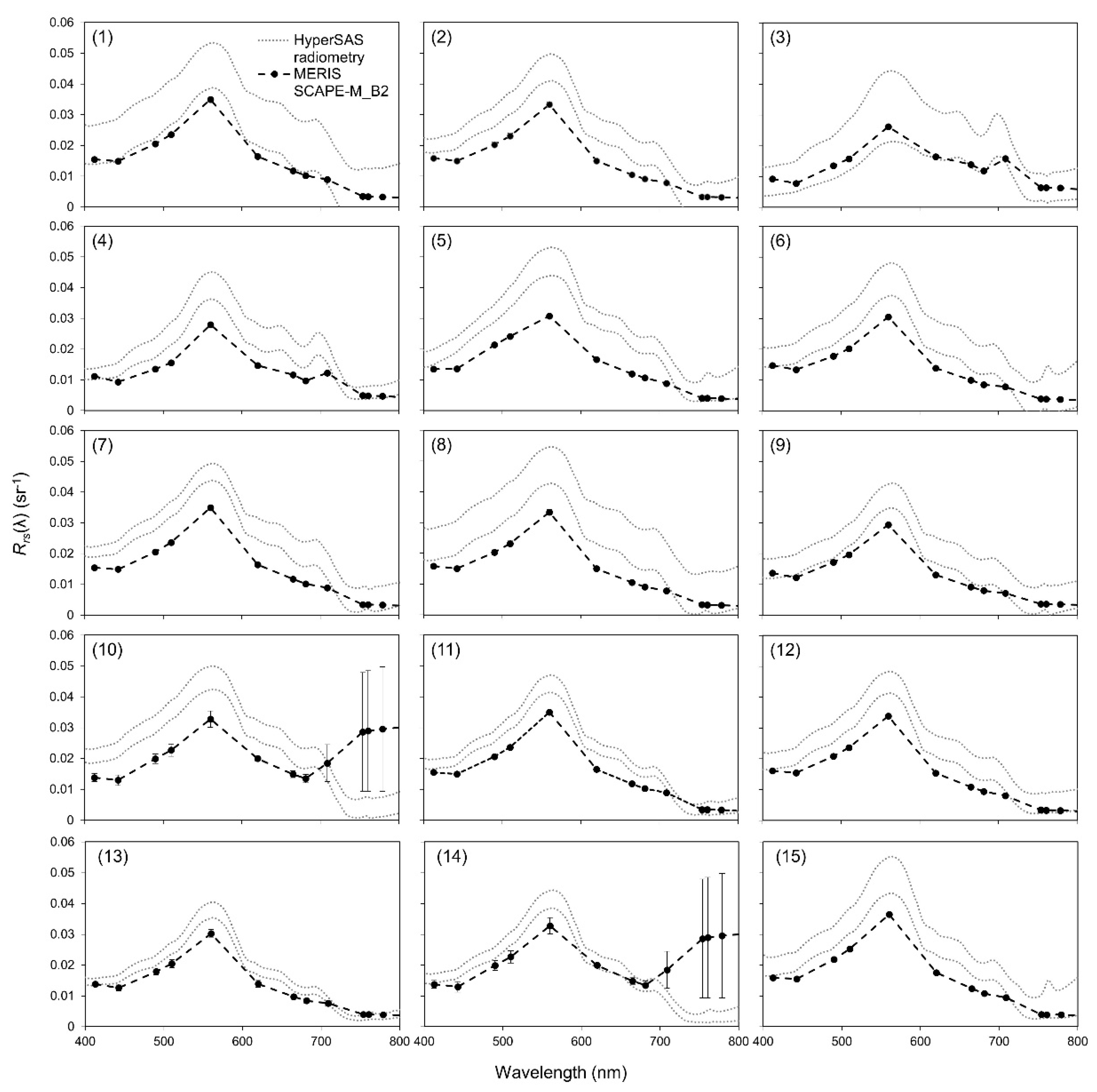
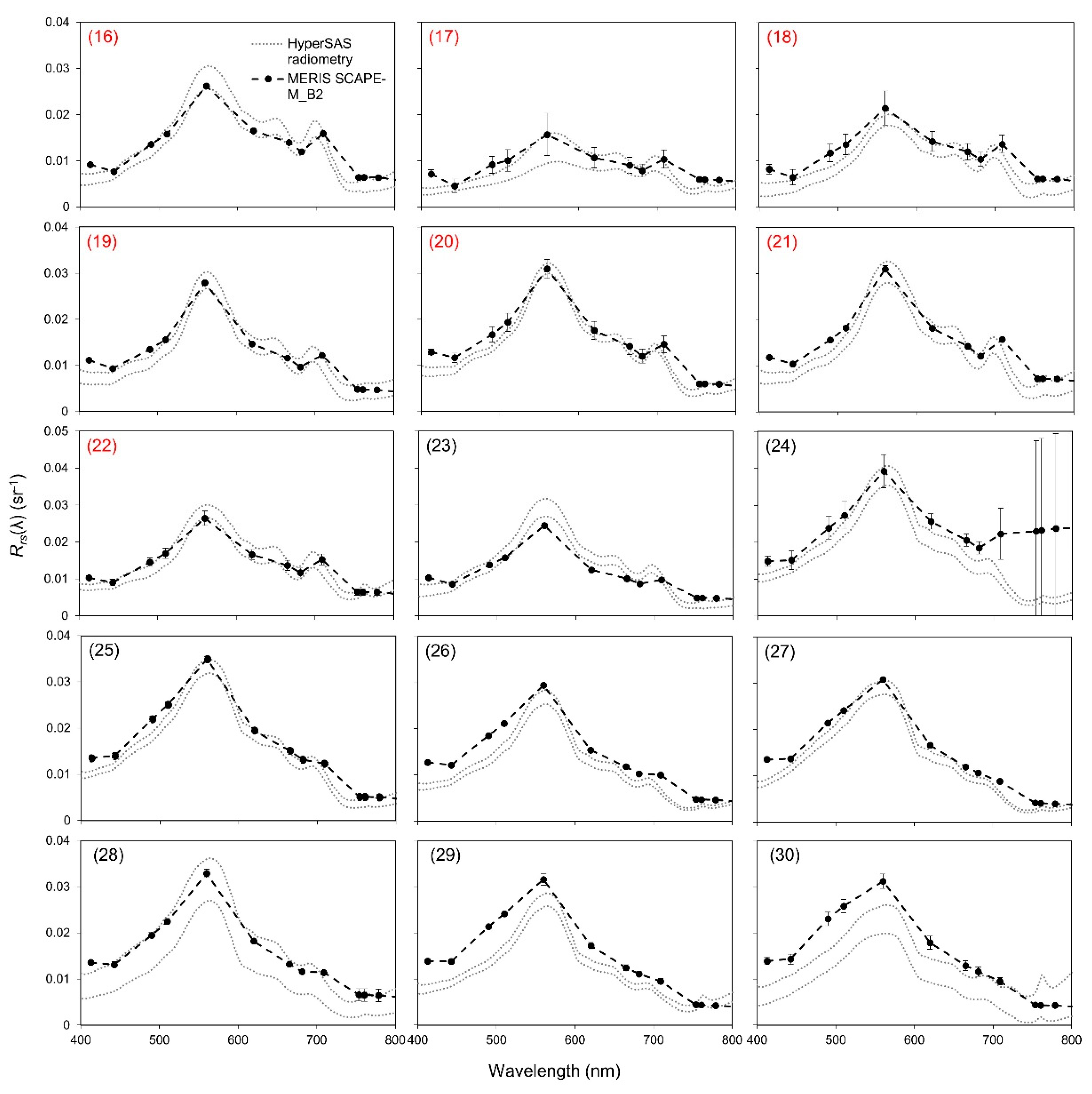
2.2.5. In Situ Radiometry
2.3. MERIS Data Processing
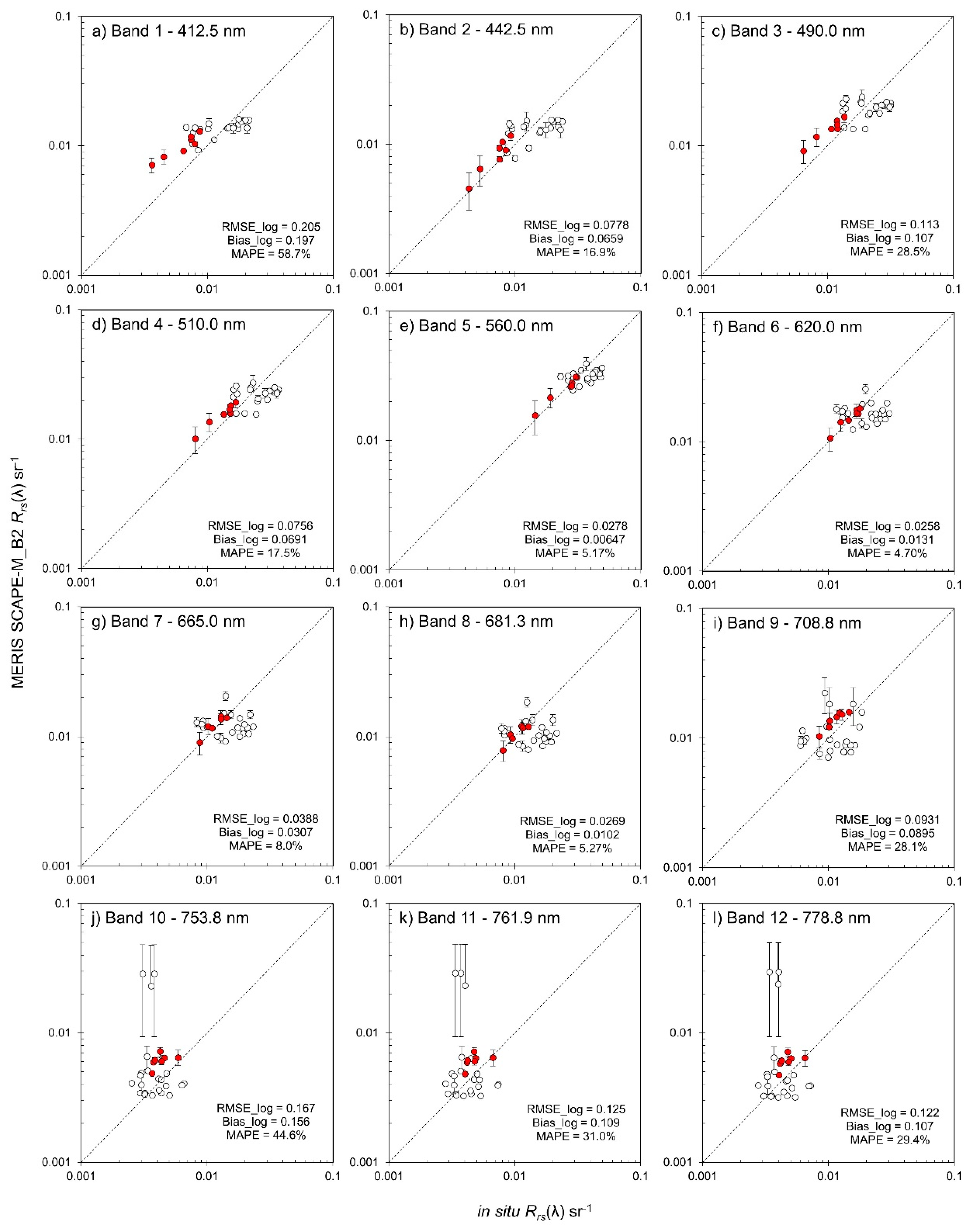
2.3.1. Validation of Atmospheric Correction
2.3.2. Validation Matchup Data
2.3.3. Algorithm Implementation and Performance Assessment
3. Results
3.1. Pigments and Cell Counts
3.2. Validation of Atmospheric Correction
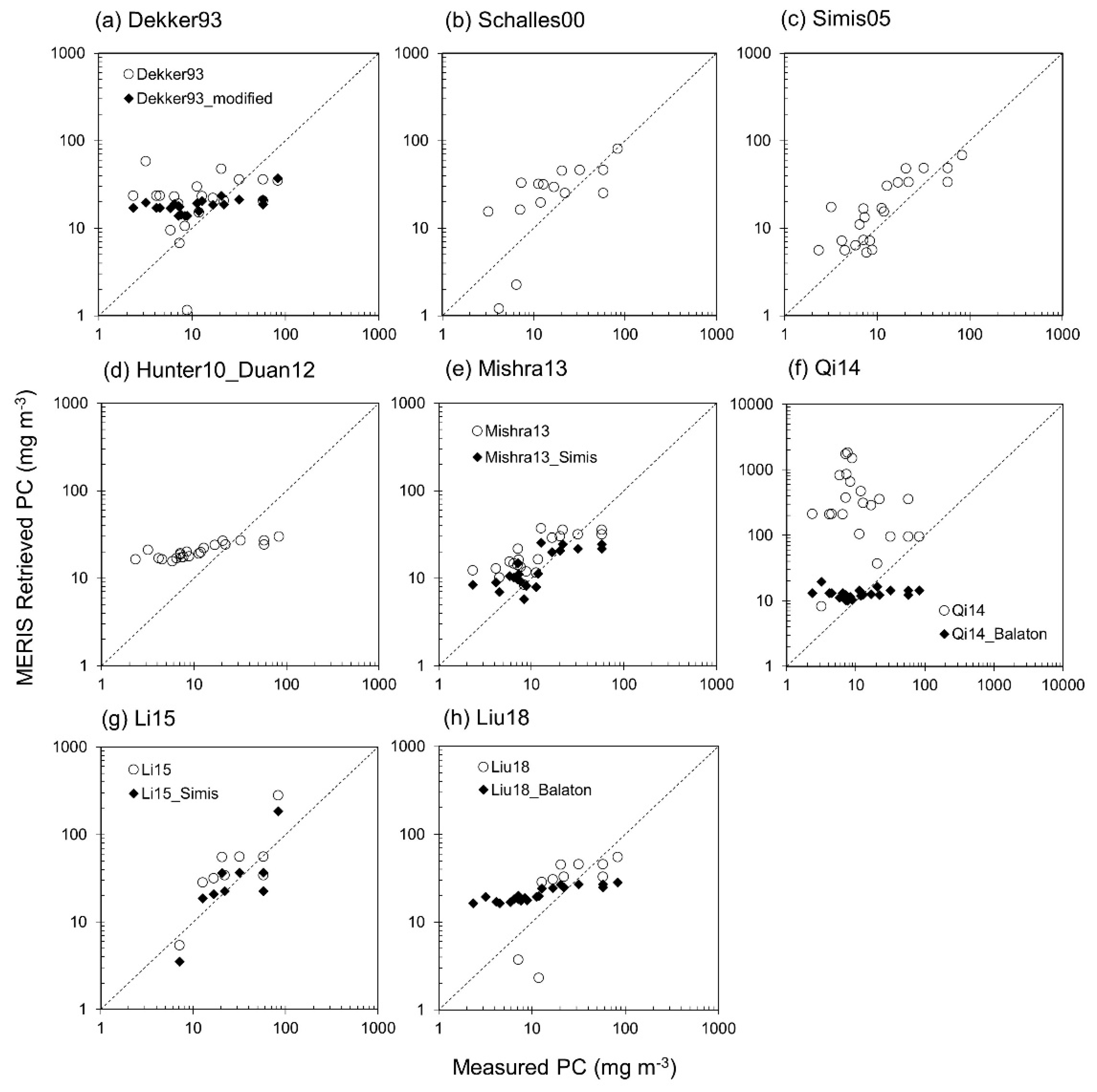
3.3. Phycocyanin Algorithm Performance
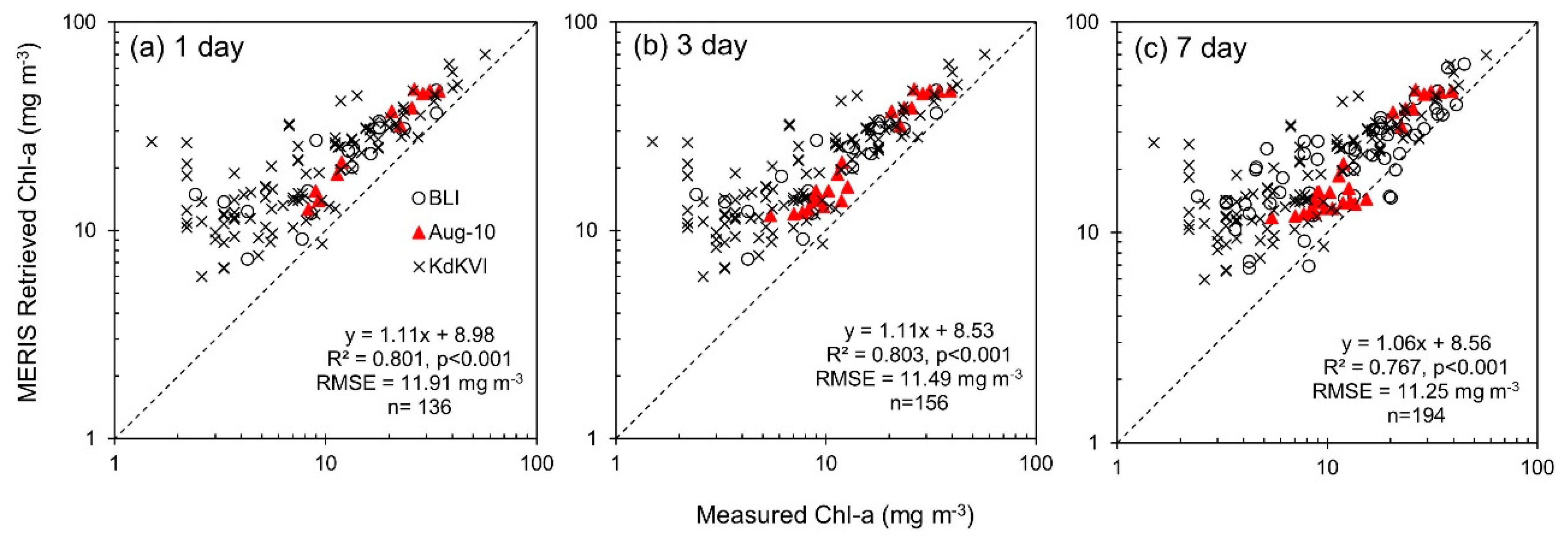
3.4. Chlorophyll-a Retrieval
3.5. Phycocyanin Retrieval
3.6. IOP Retrieval
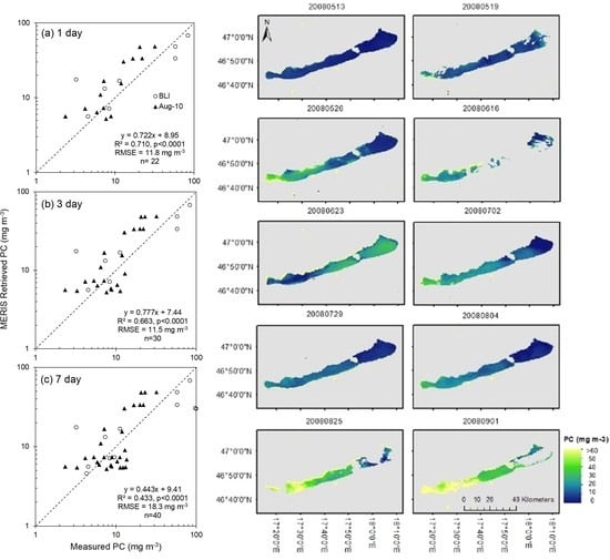
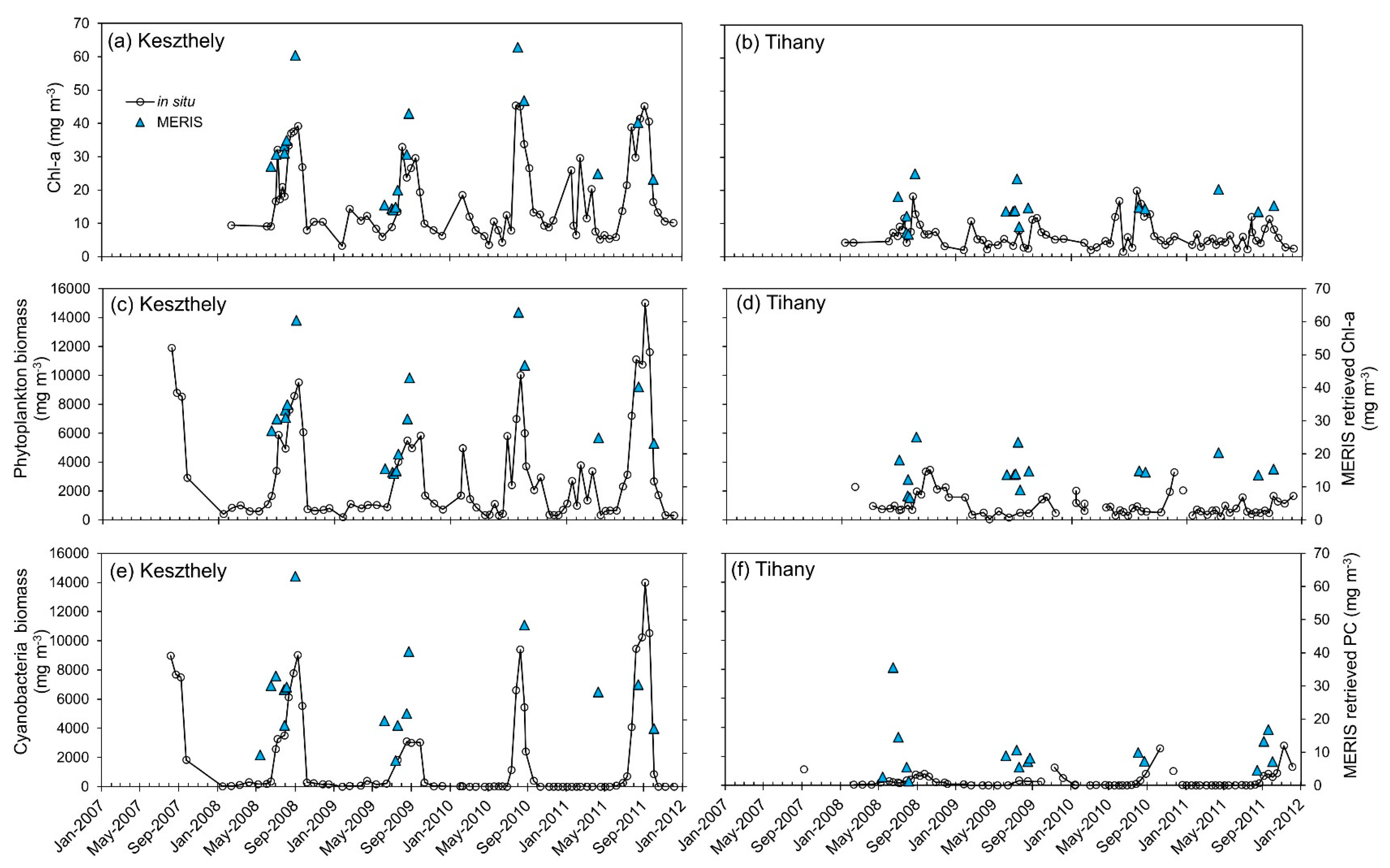
3.7. Time Series Analysis
4. Discussion
4.1. Algorithm Performance
4.2. Biomass Retrieval
4.3. Temporal Window for Validation
4.4. Impact of Dataset and Sampling Methods on Validation
4.5. Sources of Error Explained with IOP Measurements
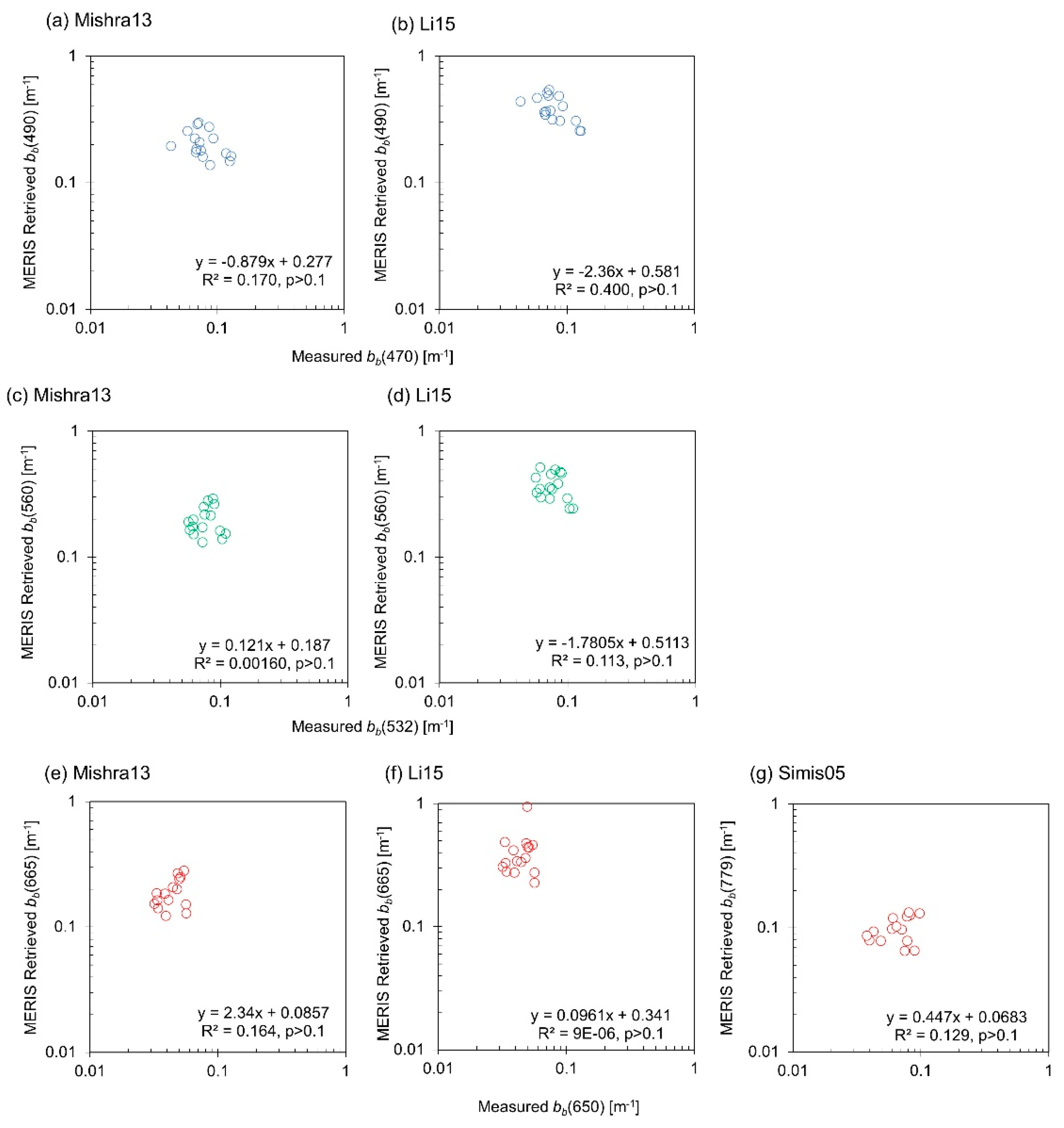
4.6. Applicability of Pigment Algorithms
5. Conclusions
Author Contributions
Funding
Acknowledgments
Conflicts of Interest
Appendix A. MERIS Phycocyanin Algorithms
Appendix A1. Dekker93
Appendix A2. Schalles00
Appendix A3. Gons05 and Simis05
Appendix A4. Hunter10_Duan
Appendix A5. Mishra13
Appendix A6. Qi14
Appendix A7. Li15
Appendix A8. Liu18
Appendix B. Validation Assessment Results

| Model | b mg m−3 | m | R2 | p | RMSE mg m−3 | RMSE log | Bias mg m−3 | Bias log | MAPE % | MdAPE % | SMAPE % |
|---|---|---|---|---|---|---|---|---|---|---|---|
| Dekker93 | 18.1 | 0.218 | 0.0992 | 0.153 | 21.6 | 0.444 | 3.94 | 0.148 | 224 | 84.4 | 88.3 |
| Dekker93_modified | 15.6 | 0.172 | 0.576 | <0.0001 | 17.5 | 0.354 | 0.614 | 0.0542 | 142 | 69.3 | 72.3 |
| Schalles00 | 4.58 | 0.822 | 0.595 | <0.0001 | 14.6 | 0.370 | 1.35 | 0.238 | 124 | 111 | 112 |
| Simis05 | 8.95 | 0.722 | 0.710 | <0.0001 | 11.8 | 0.272 | 3.92 | 0.147 | 77.0 | 50.8 | 48.2 |
| Hunter10_Duan12 | 17.9 | 0.160 | 0.662 | <0.0001 | 17.8 | 0.356 | 2.66 | 0.107 | 153 | 114 | 77.0 |
| Mishra13 | 17.3 | 0.0522 | 0.00836 | 0.686 | 22.9 | 0.330 | 0.0987 | 0.230 | 104 | 87.0 | 66.1 |
| Mishra13_Simis | 11.8 | 0.0358 | 0.00836 | 0.686 | 22.3 | 0.246 | −5.62 | 0.0664 | 61.2 | 53.2 | 58.2 |
| Qi14 | 632 | −7.68 | 0.0910 | 0.172 | 715 | 1.55 | 475 | 1.38 | 6197 | 3512 | 158 |
| Qi14_Balaton | 12.6 | 0.0211 | 0.0433 | 0.352 | 21.1 | 0.403 | −5.18 | 0.0563 | 101 | 52.8 | 64.4 |
| Li15 | −26.2 | 2.55 | 0.716 | <0.0001 | 46.3 | 0.503 | 1.84 | 0.0349 | 205 | 170 | 141 |
| Li15_Simis | −17.2 | 1.67 | 0.716 | <0.0001 | 26.4 | 0.523 | −5.00 | −0.147 | 150 | 131 | 136 |
| Liu18 | −6.40 | 0.906 | 0.634 | <0.0001 | 16.5 | 0.841 | −8.10 | −0.305 | 184 | 122 | 134 |
| Liu18_Balaton | 18.3 | 0.150 | 0.634 | <0.0001 | 18.0 | 0.354 | 2.88 | 0.088 | 155 | 113 | 78.2 |
| Model | b mg m−3 | m | R2 | p | RMSE mg m−3 | RMSE log | Bias mg m−3 | Bias log | MAPE % | MdAPE % | SMAPE % |
|---|---|---|---|---|---|---|---|---|---|---|---|
| Dekker93 | 15.0 | 0.543 | 0.0719 | 0.267 | 17.84 | 0.467 | 10.2 | 0.295 | 251 | 92.0 | 90.5 |
| Dekker93_modified | 15.7 | 0.187 | 0.281 | 0.0195 | 9.52 | 0.328 | 7.11 | 0.198 | 155 | 86.6 | 69.5 |
| Schalles00 | −4.16 | 1.78 | 0.554 | 0.117 | 13.57 | 0.405 | 4.01 | 0.357 | 139 | 124 | 124 |
| Simis05 | −0.146 | 1.69 | 0.793 | <0.0001 | 10.7 | 0.286 | 7.09 | 0.191 | 85.1 | 53.0 | 51.1 |
| Hunter10_Duan12 | 15.5 | 0.407 | 0.770 | <0.0001 | 10.4 | 0.346 | 9.28 | 0.255 | 168 | 134 | 76.0 |
| Mishra13 | 9.66 | 0.793 | 0.440 | <0.001 | 9.76 | 0.355 | 7.69 | 0.296 | 119 | 110 | 62.8 |
| Mishra13_Simis | 4.90 | 0.715 | 0.605 | <0.001 | 5.14 | 0.224 | 1.90 | 0.120 | 59.5 | 36.3 | 48.2 |
| Qi14 | 734 | −18.3 | 0.0588 | 0.317 | 766 | 1.66 | 532 | 1.54 | 7144 | 4595 | 173 |
| Qi14_Balaton | 12.3 | 0.0452 | 0.0225 | 0.539 | 7.66 | 0.339 | 2.28 | 0.172 | 105 | 43.8 | 54.0 |
| Li15 | −26.0 | 2.82 | 0.697 | <0.0001 | 20.2 | 0.561 | −6.90 | 0.00889 | 222 | 171 | 155 |
| Li15_Simis | −17.1 | 1.85 | 0.697 | <0.0001 | 13.6 | 0.587 | −8.14 | −0.173 | 162 | 146 | 147 |
| Liu18 | −21.9 | 2.51 | 0.814 | <0.0001 | 15.3 | 0.965 | −5.96 | −0.349 | 208 | 138 | 149 |
| Liu18_Balaton | 15.7 | 0.417 | 0.814 | <0.0001 | 10.6 | 0.340 | 9.56 | 0.247 | 170 | 129 | 77.4 |
| Match-up Interval | n | x | y | b mg m−3 | m | R2 | p | RMSE mg m−3 | RMSE log | Bias mg m−3 | Bias log | MAPE % | MdAPE % | SMAPE % | |
|---|---|---|---|---|---|---|---|---|---|---|---|---|---|---|---|
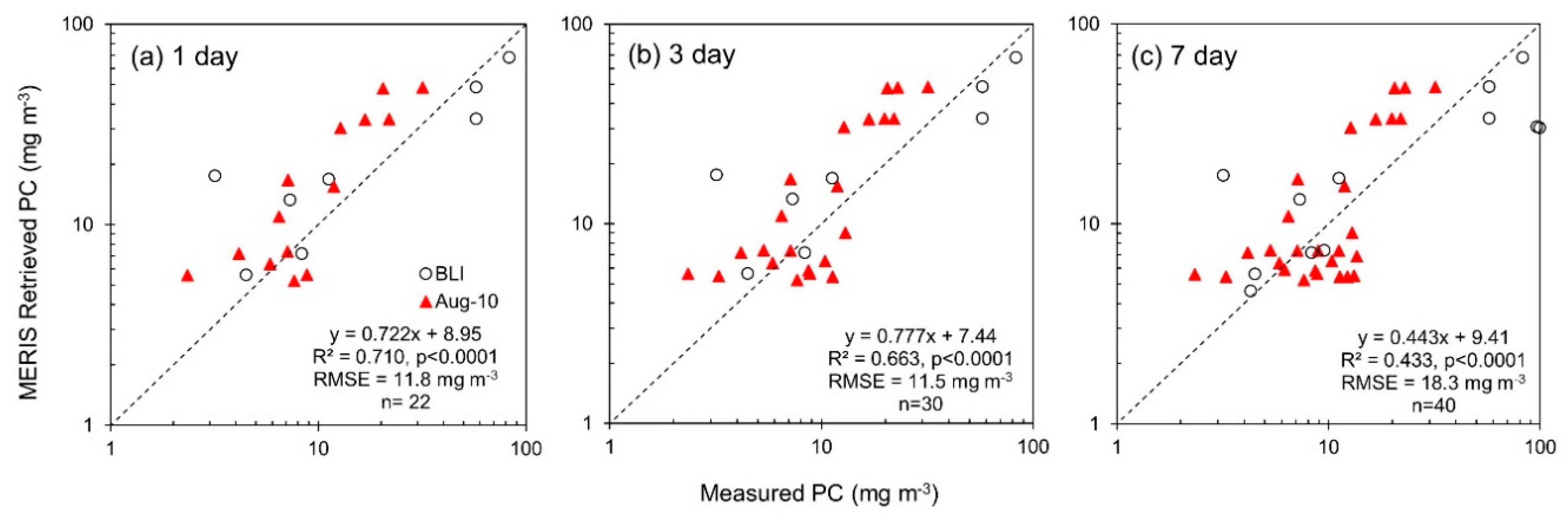
| PC | 1 day | 22 | Measured PC | MERIS Retrieved PC | 8.95 | 0.722 | 0.710 | <0.0001 | 11.8 | 0.272 | 3.92 | 0.147 | 77.0 | 50.8 | 48.2 |
| 3 day | 30 | Measured PC | MERIS Retrieved PC | 7.44 | 0.777 | 0.663 | <0.0001 | 11.5 | 0.261 | 3.77 | 0.110 | 71.0 | 50.6 | 48.5 | |
| 7 day | 40 | Measured PC | MERIS Retrieved PC | 9.41 | 0.443 | 0.433 | <0.0001 | 18.3 | 0.273 | −1.30 | 0.0218 | 63.0 | 49.5 | 49.8 | |
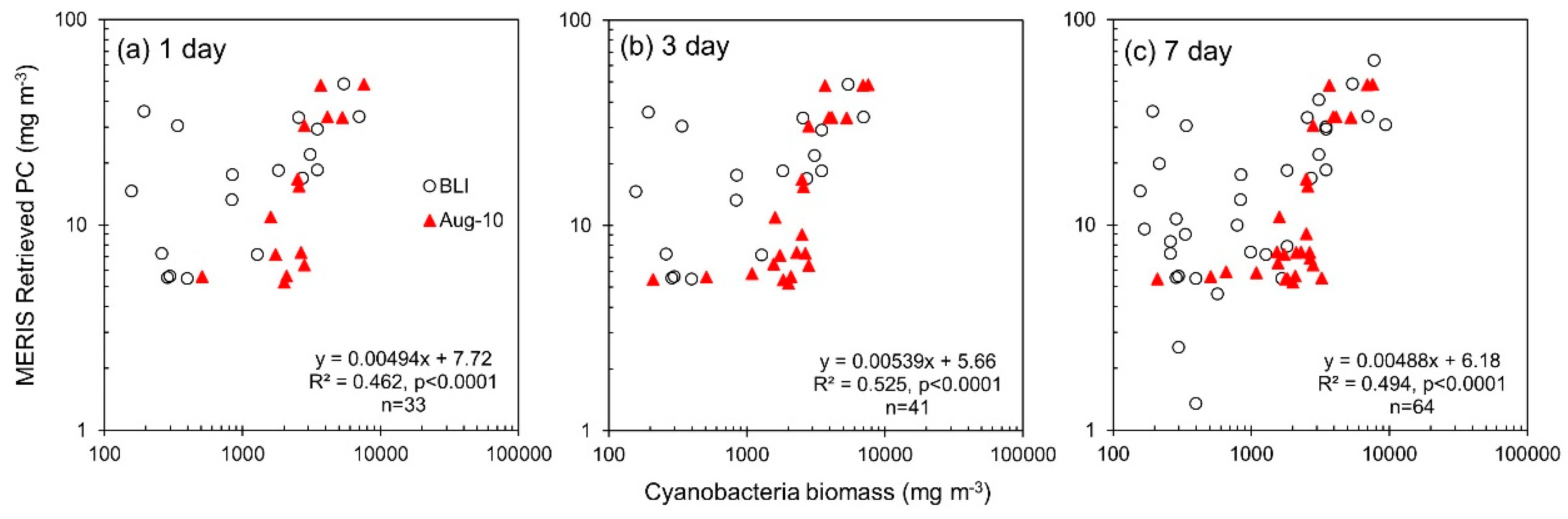
| 1 day | 33 | Cyanobacteria biomass | MERIS Retrieved PC | 7.72 | 0.00494 | 0.462 | <0.0001 | - | - | - | - | - | - | - | |
| 3 day | 41 | Cyanobacteria biomass | MERIS Retrieved PC | 5.66 | 0.00539 | 0.525 | <0.0001 | - | - | - | - | - | - | - | |
| 7 day | 64 | Cyanobacteria biomass | MERIS Retrieved PC | 6.18 | 0.00488 | 0.494 | <0.0001 | - | - | - | - | - | - | - | |
| Chl-a | 1 day | 136 | Measured Chl-a | MERIS Retrieved Chl-a | 8.98 | 1.11 | 0.801 | <0.0001 | 11.9 | 0.394 | 10.4 | 0.329 | 151 | 86.4 | 68.5 |
| 3 day | 156 | Measured Chl-a | MERIS Retrieved Chl-a | 8.53 | 1.11 | 0.803 | <0.0001 | 11.5 | 0.382 | 9.97 | 0.319 | 143 | 82.2 | 66.6 | |
| 7 day | 194 | Measured Chl-a | MERIS Retrieved Chl-a | 8.56 | 1.06 | 0.767 | <0.0001 | 11.2 | 0.369 | 9.38 | 0.296 | 132 | 74.2 | 63.0 | |
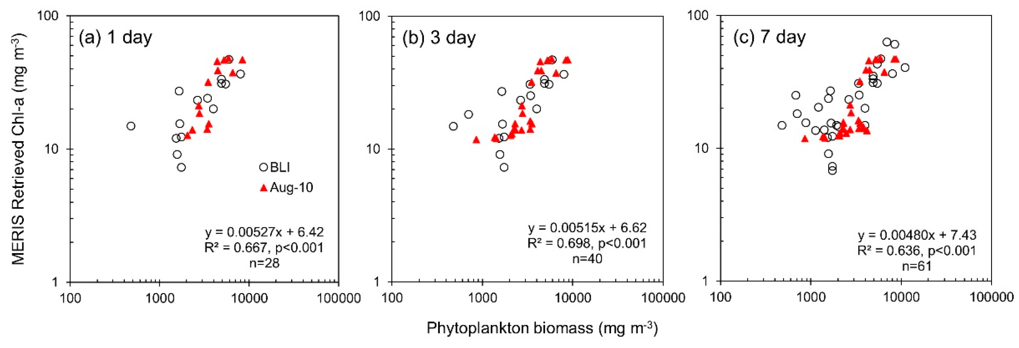
| 1 day | 28 | Phytoplankton biomass | MERIS Retrieved Chl-a | 6.42 | 0.00527 | 0.667 | <0.0001 | - | - | - | - | - | - | - | |
| 3 day | 40 | Phytoplankton biomass | MERIS Retrieved Chl-a | 6.62 | 0.00515 | 0.698 | <0.0001 | - | - | - | - | - | - | - | |
| 7 day | 61 | Phytoplankton biomass | MERIS Retrieved Chl-a | 7.43 | 0.00480 | 0.636 | <0.0001 | - | - | - | - | - | - | - |
| Match-up Interval | n | x | y | b mg m−3 or m−1 | m | R2 | p | RMSE mg m−3 or m−1 | RMSE log | Bias mg m−3 or m−1 | Bias log | MAPE % | MdAPE % | SMAPE % | |
|---|---|---|---|---|---|---|---|---|---|---|---|---|---|---|---|
| PC | 1 day | 14 | Measured PC | MERIS Retrieved PC | −1.28 | 1.77 | 0.836 | <0.0001 | 11.7 | 0.254 | 7.79 | 0.174 | 71.6 | 61.2 | 49.9 |
| 3 day | 22 | Measured PC | MERIS Retrieved PC | −4.15 | 1.87 | 0.799 | <0.0001 | 11.3 | 0.246 | 6.18 | 0.189 | 65.4 | 52.6 | 49.7 | |
| 7 day | 28 | Measured PC | MERIS Retrieved PC | −5.95 | 1.85 | 0.718 | <0.0001 | 10.3 | 0.248 | 3.89 | 0.042 | 59.3 | 52.0 | 49.4 | |
| 1 day | 14 | Cyanobacteria biomass | MERIS Retrieved PC | −2.48 | 0.00737 | 0.660 | <0.001 | - | - | - | - | - | - | - | |
| 3 day | 22 | Cyanobacteria biomass | MERIS Retrieved PC | −3.04 | 0.00743 | 0.745 | <0.0001 | - | - | - | - | - | - | - | |
| 7 day | 28 | Cyanobacteria biomass | MERIS Retrieved PC | −3.88 | 0.00731 | 0.709 | <0.0001 | - | - | - | - | - | - | - | |
| Chl-a | 1 day | 13 | Measured Chl-a | MERIS Retrieved Chl-a | 2.22 | 1.45 | 0.943 | <0.0001 | 12.2 | 0.203 | 10.9 | 0.199 | 58.9 | 52.7 | 45.0 |
| 3 day | 23 | Measured Chl-a | MERIS Retrieved Chl-a | 2.38 | 1.38 | 0.930 | <0.0001 | 10.2 | 0.198 | 8.71 | 0.189 | 55.9 | 52.7 | 42.6 | |
| 7 day | 29 | Measured Chl-a | MERIS Retrieved Chl-a | 0.995 | 1.41 | 0.906 | <0.0001 | 9.19 | 0.185 | 7.36 | 0.167 | 50 | 50.6 | 38.1 | |
| 1 day | 13 | Phytoplankton biomass | MERIS Retrieved Chl-a | 3.24 | 0.00633 | 0.656 | <0.001 | - | - | - | - | - | - | - | |
| 3 day | 23 | Phytoplankton biomass | MERIS Retrieved Chl-a | 3.88 | 0.00588 | 0.736 | <0.0001 | - | - | - | - | - | - | - | |
| 7 day | 29 | Phytoplankton biomass | MERIS Retrieved Chl-a | 2.22 | 0.00587 | 0.682 | <0.0001 | - | - | - | - | - | - | - | |
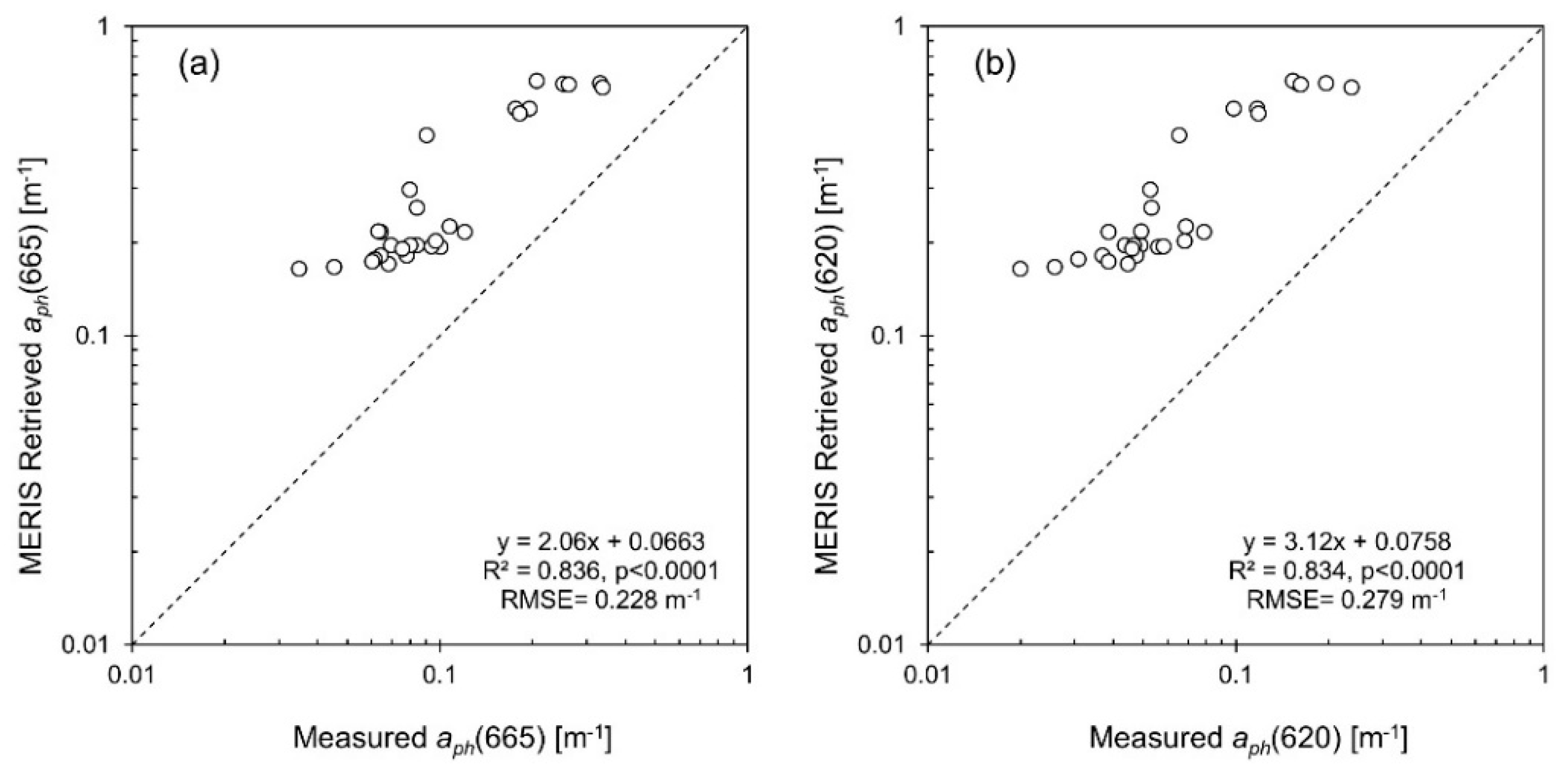
| aph (665) | 7 day | 29 | Measured aph(665) | MERIS Retrieved aph(665) | 0.0663 | 2.06 | 0.836 | <0.0001 | 0.228 | 0.444 | 0.197 | 0.430 | 178 | 175 | 90.6 |
| aph (620) | 7 day | 29 | Measured aph(620) | MERIS Retrieved aChla+PC (620) | 0.0758 | 3.12 | 0.834 | <0.0001 | 0.279 | 0.645 | 0.242 | 0.635 | 346 | 332 | 123 |
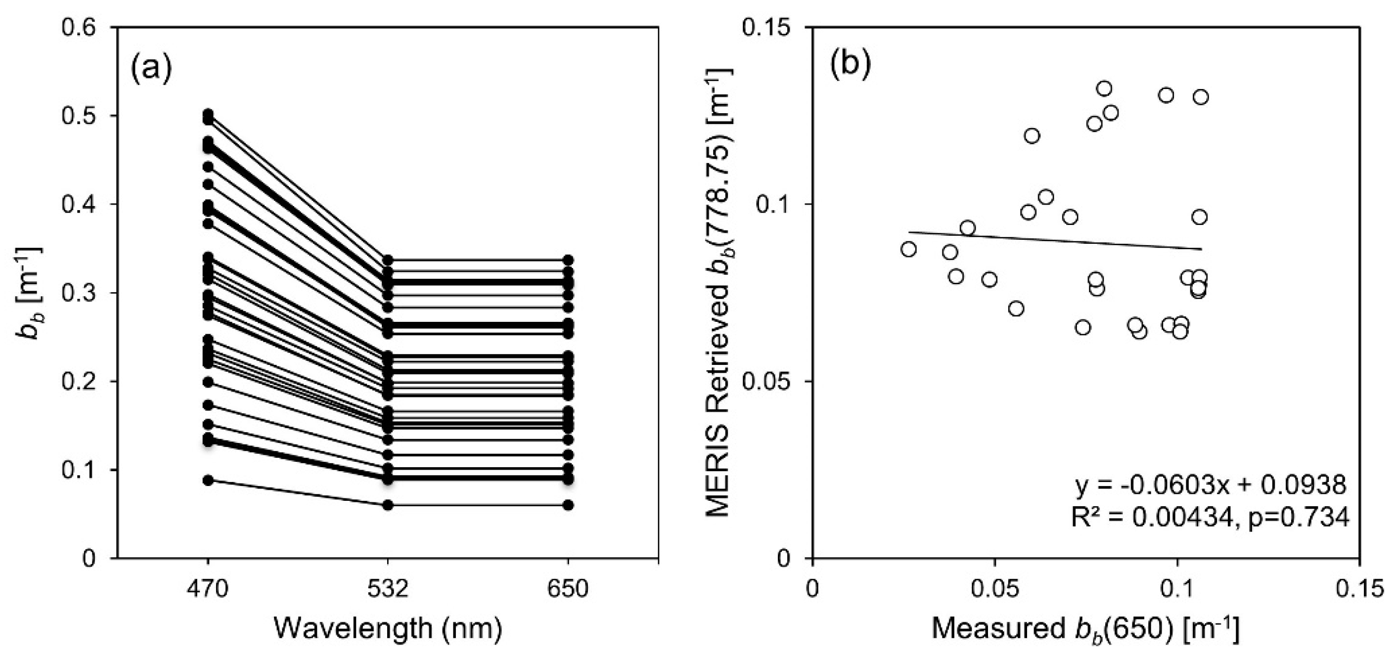
| bb (λ) | 7 day | 29 | Measured bb(650) | MERIS Retrieved bb(778.75) | 0.0938 | −0.0603 | 0.00434 | 0.734 | - | - | - | - | - | - | - |
| Match-up Interval | n | x | y | b mg m−3 | m | R2 | p | RMSE mg m−3 | RMSE log | Bias mg m−3 | Bias log | MAPE % | MdAPE % | SMAPE % | |
|---|---|---|---|---|---|---|---|---|---|---|---|---|---|---|---|
| PC | 1 day | 8 | Measured PC | MERIS Retrieved PC | 6.94 | 0.664 | 0.910 | <0.001 | 12.1 | 0.301 | −2.86 | 0.100 | 86.4 | 33.1 | 45.4 |
| 3 day | 8 | Measured PC | MERIS Retrieved PC | 6.94 | 0.664 | 0.910 | <0.001 | 12.1 | 0.301 | −2.86 | 0.100 | 86.4 | 33.1 | 45.4 | |
| 7 day | 12 | Measured PC | MERIS Retrieved PC | 9.55 | 0.379 | 0.580 | <0.01 | 29.5 | 0.324 | −13.4 | −0.026 | 71.7 | 33.1 | 50.7 | |
| 1 day | 19 | Cyanobacteria biomass | MERIS Retrieved PC | 11.2 | 0.00421 | 0.405 | <0.01 | - | - | - | - | - | - | - | |
| 3 day | 19 | Cyanobacteria biomass | MERIS Retrieved PC | 11.2 | 0.00421 | 0.405 | <0.01 | - | - | - | - | - | - | - | |
| 7 day | 36 | Cyanobacteria biomass | MERIS Retrieved PC | 10.1 | 0.00430 | 0.474 | <0.0001 | - | - | - | - | - | - | - | |
| Chl-a | 1 day | 18 | Measured Chl-a | MERIS Retrieved Chl-a | 8.26 | 1.03 | 0.810 | <0.0001 | 9.73 | 0.331 | 8.60 | 0.271 | 109 | 70.6 | 57.5 |
| 3 day | 20 | Measured Chl-a | MERIS Retrieved Chl-a | 8.81 | 1.02 | 0.798 | <0.0001 | 10.2 | 0.337 | 9.09 | 0.281 | 112 | 76.5 | 59.9 | |
| 7 day | 52 | Measured Chl-a | MERIS Retrieved Chl-a | 9.12 | 0.950 | 0.723 | <0.0001 | 10.7 | 0.334 | 8.33 | 0.249 | 107 | 61.5 | 55.7 | |
| 1 day | 15 | Phytoplankton biomass | MERIS Retrieved Chl-a | 8.27 | 0.00438 | 0.692 | <0.001 | - | - | - | - | - | - | - | |
| 3 day | 17 | Phytoplankton biomass | MERIS Retrieved Chl-a | 9.82 | 0.00417 | 0.660 | <0.0001 | - | - | - | - | - | - | - | |
| 7 day | 37 | Phytoplankton biomass | MERIS Retrieved Chl-a | 10.3 | 0.00432 | 0.640 | <0.0001 | - | - | - | - | - | - | - |
| Match-up Interval | n | x | y | b mg m−3 | m | R2 | p | RMSE mg m−3 | RMSE log | Bias mg m−3 | Bias log | MAPE % | MdAPE % | SMAPE % | |
|---|---|---|---|---|---|---|---|---|---|---|---|---|---|---|---|
| Chl-a | 1 day | 105 | Measured Chl-a | MERIS Retrieved Chl-a | 9.52 | 1.09 | 0.784 | <0.0001 | 12.2 | 0.421 | 10.6 | 0.355 | 169 | 101 | 73.3 |
| 3 day | 113 | Measured Chl-a | MERIS Retrieved Chl-a | 9.27 | 1.09 | 0.786 | <0.0001 | 12.0 | 0.416 | 10.4 | 0.352 | 165 | 101 | 72.7 | |
| 7 day | 113 | Measured Chl-a | MERIS Retrieved Chl-a | 9.27 | 1.09 | 0.786 | <0.0001 | 12.0 | 0.416 | 10.4 | 0.352 | 165 | 101 | 72.7 |
| Match-up Interval | n | x | y | b mg m−3 | m | R2 | p | RMSE mg m−3 | RMSE log | Bias mg m−3 | Bias log | MAPE % | MdAPE % | SMAPE % | |
|---|---|---|---|---|---|---|---|---|---|---|---|---|---|---|---|
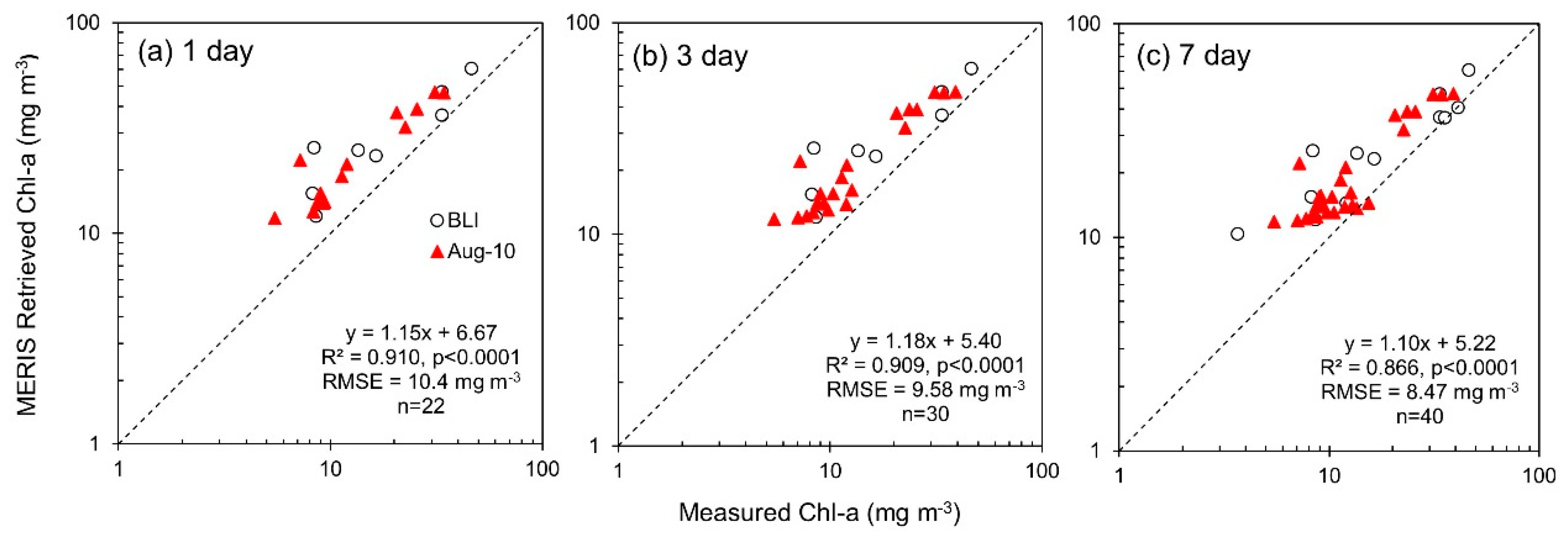
| Chl-a | 1 day | 22 | Measured Chl-a | MERIS Retrieved Chl-a | 6.67 | 1.15 | 0.910 | <0.0001 | 10.4 | 0.241 | 9.33 | 0.216 | 70.0 | 51.9 | 48.0 |
| 3 day | 30 | Measured Chl-a | MERIS Retrieved Chl-a | 5.40 | 1.18 | 0.909 | <0.0001 | 9.58 | 0.222 | 8.39 | 0.199 | 62.7 | 50.9 | 44.3 | |
| 7 day | 40 | Measured Chl-a | MERIS Retrieved Chl-a | 5.22 | 1.10 | 0.866 | <0.0001 | 8.47 | 0.211 | 6.84 | 0.174 | 55.9 | 50.1 | 39.2 |


References
- Verpoorter, C.; Kutser, T.; Seekell, D.A.; Tranvik, L.J. A global inventory of lakes based on high-resolution satellite imagery. Geophys. Res. Lett. 2014, 41, 6396–6402. [Google Scholar] [CrossRef]
- Bastviken, D.; Tranvik, L.J.; Downing, J.A.; Crill, P.M.; Enrich-Prast, A. Freshwater Methane Emissions Offset the Continental Carbon Sink. Science 2011, 331, 50. [Google Scholar] [CrossRef] [PubMed]
- Cole, J.J.; Prairie, Y.T.; Caraco, N.F.; McDowell, W.H.; Tranvik, L.J.; Striegl, R.G.; Duarte, C.M.; Kortelainen, P.; Downing, J.A.; Middelburg, J.J.; et al. Plumbing the Global Carbon Cycle: Integrating Inland Waters into the Terrestrial Carbon Budget. Ecosystems 2007, 10, 172–185. [Google Scholar] [CrossRef] [Green Version]
- Smith, V.H. Eutrophication of freshwater and coastal marine ecosystems a global problem. Environ. Sci. Pollut. Res. 2003, 10, 126–139. [Google Scholar] [CrossRef]
- Fink, G.; Alcamo, J.; Flörke, M.; Reder, K. Phosphorus Loadings to the World’s Largest Lakes: Sources and Trends. Glob. Biogeochem. Cycles 2018, 32, 617–634. [Google Scholar] [CrossRef]
- Paerl, H.W.; Hall, N.S.; Calandrino, E.S. Controlling harmful cyanobacterial blooms in a world experiencing anthropogenic and climatic-induced change. Sci. Total Environ. 2011, 409, 1739–1745. [Google Scholar] [CrossRef] [PubMed]
- Downing, J.A.; Watson, S.B.; McCauley, E. Predicting Cyanobacteria dominance in lakes. Can. J. Fish. Aquat. Sci. 2001, 58, 1905–1908. [Google Scholar] [CrossRef]
- Ferber, L.R.; Levine, S.N.; Lini, A.; Livingston, G.P. Do cyanobacteria dominate in eutrophic lakes because they fix atmospheric nitrogen? Freshw. Biol. 2004, 49, 690–708. [Google Scholar] [CrossRef]
- Horváth, H.; Kovács, A.W.; Riddick, C.; Présing, M. Extraction methods for phycocyanin determination in freshwater filamentous cyanobacteria and their application in a shallow lake. Eur. J. Phycol. 2013, 48, 278–286. [Google Scholar] [CrossRef] [Green Version]
- Présing, M.; Preston, T.; Takátsy, A.; Sprőber, P.; Kovács, A.W.; Vörös, L.; Kenesi, G.; Kóbor, I. Phytoplankton nitrogen demand and the significance of internal and external nitrogen sources in a large shallow lake (Lake Balaton, Hungary). Hydrobiologia 2008, 599, 87–95. [Google Scholar] [CrossRef]
- Schindler, D.W. Evolution of Phosphorus Limitation in Lakes. Science 1977, 195, 260–262. [Google Scholar] [CrossRef] [PubMed] [Green Version]
- Smith, V.H. Low Nitrogen to Phosphorus Ratios Favor Dominance by Blue-Green Algae in Lake Phytoplankton. Science 1983, 221, 669–671. [Google Scholar] [CrossRef] [PubMed] [Green Version]
- Antenucci, J.P.; Ghadouani, A.; Burford, M.A.; Romero, J.R. The long-term effect of artificial destratification on phytoplankton species composition in a subtropical reservoir. Freshw. Biol. 2005, 50, 1081–1093. [Google Scholar] [CrossRef]
- Reynolds, C.S.; Huszar, V.; Kruk, C.; Naselli-Flores, L.; Melo, S. Towards a functional classification of the freshwater phytoplankton. J. Plankton Res. 2002, 24, 417–428. [Google Scholar] [CrossRef]
- Paerl, H.W.; Huisman, J. Climate change: a catalyst for global expansion of harmful cyanobacterial blooms. Environ. Microbiol. Rep. 2009, 1, 27–37. [Google Scholar] [CrossRef]
- Wagner, C.; Adrian, R. Cyanobacteria dominance: Quantifying the effects of climate change. Limnol. Oceanogr. 2009, 54, 2460–2468. [Google Scholar] [CrossRef]
- Codd, G.A.; Morrison, L.F.; Metcalf, J.S. Cyanobacterial toxins: risk management for health protection. Toxicol. Appl. Pharmacol. 2005, 203, 264–272. [Google Scholar] [CrossRef]
- Palmer, S.C.J.; Kutser, T.; Hunter, P.D. Remote sensing of inland waters: Challenges, progress and future directions. Remote Sens. Environ. 2015, 157, 1–8. [Google Scholar] [CrossRef] [Green Version]
- Gons, H.J.; Rijkeboer, M.; Ruddick, K.G. A chlorophyll-retrieval algorithm for satellite imagery (Medium Resolution Imaging Spectrometer) of inland and coastal waters. J. Plankton Res. 2002, 24, 947–951. [Google Scholar] [CrossRef] [Green Version]
- Kutser, T. Quantitative detection of chlorophyll in cyanobacterial blooms by satellite remote sensing. Limnol. Oceanogr. 2004, 49, 2179–2189. [Google Scholar] [CrossRef]
- Tyler, A.N.; Svab, E.; Preston, T.; Présing, M.; Kovács, W.A. Remote sensing of the water quality of shallow lakes: A mixture modelling approach to quantifying phytoplankton in water characterized by high-suspended sediment. Int. J. Remote Sens. 2006, 27, 1521–1537. [Google Scholar] [CrossRef]
- Duan, H.; Ma, R.; Hu, C. Evaluation of remote sensing algorithms for cyanobacterial pigment retrievals during spring bloom formation in several lakes of East China. Remote Sens. Environ. 2012, 126, 126–135. [Google Scholar] [CrossRef]
- Hunter, P.D.; Tyler, A.N.; Carvalho, L.; Codd, G.A.; Maberly, S.C. Hyperspectral remote sensing of cyanobacterial pigments as indicators for cell populations and toxins in eutrophic lakes. Remote Sens. Environ. 2010, 114, 2705–2718. [Google Scholar] [CrossRef] [Green Version]
- Kutser, T. Passive optical remote sensing of cyanobacteria and other intense phytoplankton blooms in coastal and inland waters. Int. J. Remote Sens. 2009, 30, 4401–4425. [Google Scholar] [CrossRef]
- Kutser, T.; Metsamaa, L.; Strömbeck, N.; Vahtmäe, E. Monitoring cyanobacterial blooms by satellite remote sensing. Estuar. Coast. Shelf Sci. 2006, 67, 303–312. [Google Scholar] [CrossRef]
- Li, L.; Li, L.; Shi, K.; Li, Z.; Song, K. A semi-analytical algorithm for remote estimation of phycocyanin in inland waters. Sci. Total Environ. 2012, 435–436, 141–150. [Google Scholar] [CrossRef] [PubMed]
- Ruiz-Verdú, A.; Simis, S.G.H.; de Hoyos, C.; Gons, H.J.; Peña-Martínez, R. An evaluation of algorithms for the remote sensing of cyanobacterial biomass. Remote Sens. Environ. 2008, 112, 3996–4008. [Google Scholar] [CrossRef]
- Simis, S.G.H.; Peters, S.W.M.; Gons, H.J. Remote sensing of the cyanobacterial pigment phycocyanin in turbid inland water. Limnol. Oceanogr. 2005, 50, 237–245. [Google Scholar] [CrossRef]
- Song, K.; Li, L.; Tedesco, L.; Clercin, N.; Hall, B.; Li, S.; Shi, K.; Liu, D.; Sun, Y. Remote estimation of phycocyanin (PC) for inland waters coupled with YSI PC fluorescence probe. Environ. Sci. Pollut. Res. 2013, 20, 5330–5340. [Google Scholar] [CrossRef]
- Hunter, P.; Tyler, A.; Presing, M.; Kovacs, A.; Preston, T. Spectral discrimination of phytoplankton colour groups: The effect of suspended particulate matter and sensor spectral resolution. Remote Sens. Environ. 2008, 112, 1527–1544. [Google Scholar] [CrossRef]
- Dekker, A.G. Detection of Optical Water Quality Parameters for Eutrophic Waters by High Resolution Remote Sensing. Ph.D. Thesis, Proefschrift Vrije Universiteit (Free University), Amsterdam, The Netherlands, 1993. [Google Scholar]
- Schalles, J.F.; Yacobi, Y.Z. Remote detection and seasonal patterns of phycocyanin, carotenoid and chlorophyll pigments in eutrophic waters. Ergeb. Limnol. 2000, 55, 153–168. [Google Scholar]
- Gons, H.J. Optical Teledetection of Chlorophyll a in Turbid Inland Waters. Environ. Sci. Technol. 1999, 33, 1127–1132. [Google Scholar] [CrossRef]
- Gons, H.J.; Rijkeboer, M.; Ruddick, K.G. Effect of a waveband shift on chlorophyll retrieval from MERIS imagery of inland and coastal waters. J. Plankton Res. 2005, 27, 125–127. [Google Scholar] [CrossRef]
- Le, C.; Li, Y.; Zha, Y.; Wang, Q.; Zhang, H.; Yin, B. Remote sensing of phycocyanin pigment in highly turbid inland waters in Lake Taihu, China. Int. J. Remote Sens. 2011, 32, 8253–8269. [Google Scholar] [CrossRef]
- Randolph, K.; Wilson, J.; Tedesco, L.; Li, L.; Pascual, D.L.; Soyeux, E. Hyperspectral remote sensing of cyanobacteria in turbid productive water using optically active pigments, chlorophyll a and phycocyanin. Remote Sens. Environ. 2008, 112, 4009–4019. [Google Scholar] [CrossRef]
- Simis, S.G.H.; Ruiz-Verdú, A.; Domínguez-Gómez, J.A.; Peña-Martinez, R.; Peters, S.W.M.; Gons, H.J. Influence of phytoplankton pigment composition on remote sensing of cyanobacterial biomass. Remote Sens. Environ. 2007, 106, 414–427. [Google Scholar] [CrossRef]
- Wheeler, S.M.; Morrissey, L.A.; Levine, S.N.; Livingston, G.P.; Vincent, W.F. Mapping cyanobacterial blooms in Lake Champlain’s Missisquoi Bay using QuickBird and MERIS satellite data. J. Gt. Lakes Res. 2012, 38, 68–75. [Google Scholar] [CrossRef]
- Mishra, S.; Mishra, D.R.; Lee, Z.; Tucker, C.S. Quantifying cyanobacterial phycocyanin concentration in turbid productive waters: A quasi-analytical approach. Remote Sens. Environ. 2013, 133, 141–151. [Google Scholar] [CrossRef]
- Qi, L.; Hu, C.; Duan, H.; Cannizzaro, J.; Ma, R. A novel MERIS algorithm to derive cyanobacterial phycocyanin pigment concentrations in a eutrophic lake: Theoretical basis and practical considerations. Remote Sens. Environ. 2014, 154, 298–317. [Google Scholar] [CrossRef]
- Li, L.; Li, L.; Song, K. Remote sensing of freshwater cyanobacteria: An extended IOP Inversion Model of Inland Waters (IIMIW) for partitioning absorption coefficient and estimating phycocyanin. Remote Sens. Environ. 2015, 157, 9–23. [Google Scholar] [CrossRef]
- Liu, G.; Simis, S.G.H.; Li, L.; Wang, Q.; Li, Y.; Song, K.; Lyu, H.; Zheng, Z.; Shi, K. A Four-Band Semi-Analytical Model for Estimating Phycocyanin in Inland Waters From Simulated MERIS and OLCI Data. IEEE Trans. Geosci. Remote Sens. 2018, 56, 1374–1385. [Google Scholar] [CrossRef]
- Matthews, M.W. A current review of empirical procedures of remote sensing in inland and near-coastal transitional waters. Int. J. Remote Sens. 2011, 32, 6855–6899. [Google Scholar] [CrossRef]
- Li, L.; Song, K. Bio-optical Modeling of Phycocyanin. In Bio-optical Modeling and Remote Sensing of Inland Waters; Elsevier: Amsterdam, The Netherlands, 2017; pp. 233–262. ISBN 978-0-12-804644-9. [Google Scholar]
- Yan, Y.; Bao, Z.; Shao, J. Phycocyanin concentration retrieval in inland waters: A comparative review of the remote sensing techniques and algorithms. J. Gt. Lakes Res. 2018, 44, 748–755. [Google Scholar] [CrossRef]
- Blix, K.; Pálffy, K.; Tóth, V.R.; Eltoft, T. Remote Sensing of Water Quality Parameters over Lake Balaton by Using Sentinel-3 OLCI. Water 2018, 10, 1428. [Google Scholar] [CrossRef]
- Mouw, C.B.; Greb, S.; Aurin, D.; DiGiacomo, P.M.; Lee, Z.; Twardowski, M.; Binding, C.; Hu, C.; Ma, R.; Moore, T.; et al. Aquatic color radiometry remote sensing of coastal and inland waters: Challenges and recommendations for future satellite missions. Remote Sens. Environ. 2015, 160, 15–30. [Google Scholar] [CrossRef]
- Tyler, A.N.; Hunter, P.D.; Spyrakos, E.; Groom, S.; Constantinescu, A.M.; Kitchen, J. Developments in Earth observation for the assessment and monitoring of inland, transitional, coastal and shelf-sea waters. Sci. Total Environ. 2016, 572, 1307–1321. [Google Scholar] [CrossRef] [PubMed] [Green Version]
- Ogashawara, I.; Mishra, D.; Mishra, S.; Curtarelli, M.; Stech, J. A Performance Review of Reflectance Based Algorithms for Predicting Phycocyanin Concentrations in Inland Waters. Remote Sens. 2013, 5, 4774–4798. [Google Scholar] [CrossRef] [Green Version]
- Beck, R.; Xu, M.; Zhan, S.; Liu, H.; Johansen, R.; Tong, S.; Yang, B.; Shu, S.; Wu, Q.; Wang, S.; et al. Comparison of Satellite Reflectance Algorithms for Estimating Phycocyanin Values and Cyanobacterial Total Biovolume in a Temperate Reservoir Using Coincident Hyperspectral Aircraft Imagery and Dense Coincident Surface Observations. Remote Sens. 2017, 9, 538. [Google Scholar] [CrossRef]
- Riddick, C.A.L.; Hunter, P.D.; Tyler, A.N.; Martinez-Vicente, V.; Horváth, H.; Kovács, A.W.; Vörös, L.; Preston, T.; Présing, M. Spatial variability of absorption coefficients over a biogeochemical gradient in a large and optically complex shallow lake: LIGHT ABSORPTION IN LAKE BALATON. J. Geophys. Res. Oceans 2015, 120, 7040–7066. [Google Scholar] [CrossRef]
- Aulló-Maestro, M.E.; Hunter, P.; Spyrakos, E.; Mercatoris, P.; Kovács, A.; Horváth, H.; Preston, T.; Présing, M.; Torres Palenzuela, J.; Tyler, A. Spatio-seasonal variability of chromophoric dissolved organic matter absorption and responses to photobleaching in a large shallow temperate lake. Biogeosciences 2017, 14, 1215–1233. [Google Scholar] [CrossRef] [Green Version]
- Iwamura, T.; Nagai, H.; Ichimura, S.-E. Improved Methods for Determining Contents of Chlorophyll, Protein, Ribonucleic Acid, and Deoxyribonucleic Acid in Planktonic Populations. Int. Revue ges. Hydrobiol. Hydrogr. 1970, 55, 131–147. [Google Scholar] [CrossRef]
- Palmer, S.C.J.; Hunter, P.D.; Lankester, T.; Hubbard, S.; Spyrakos, E.; Tyler, A.N.; Présing, M.; Horváth, H.; Lamb, A.; Balzter, H.; et al. Validation of Envisat MERIS algorithms for chlorophyll retrieval in a large, turbid and optically-complex shallow lake. Remote Sens. Environ. 2015, 157, 158–169. [Google Scholar] [CrossRef] [Green Version]
- Sarada, R.; Pillai, M.G.; Ravishankar, G.A. Phycocyanin from Spirulina sp: influence of processing of biomass on phycocyanin yield, analysis of efficacy of extraction methods and stability studies on phycocyanin. Process Biochem. 1999, 34, 795–801. [Google Scholar] [CrossRef]
- Siegelman, H.; Kycia, J.H. Algal biliproteins. In Handbook of Phycological Methods: Physiological and Biochemical Methods; Hellebust, J.A., Craigie, J.S., Eds.; Cambridge University Press: New York, NY, USA, 1978; pp. 71–79. [Google Scholar]
- Utermöhl, H. Zur Vervollkommnung der quantitativen Phytoplankton-Methodik; Schweizerbart: Stuttgart, Germany, 1958. [Google Scholar]
- Németh, J.; Vörös, L. Koncepció és módszertan felszíni vizek algológiai monitoringjához [Concepts and methodics for algological monitoring of surface water]. In Környezetés természetvédelmi kutatások; Katona, S., Ed.; Országos Környezet és Termeszetvédelmi Hivatal: Budapest, Hungary, 1986; ISBN 978-963-02-4647-7. [Google Scholar]
- Tassan, S.; Ferrari, G.M. Measurement of light absorption by aquatic particles retained on filters: determination of the optical pathlength amplification by the ‘transmittance-reflectance’ method. J. Plankton Res. 1998, 20, 1699–1709. [Google Scholar] [CrossRef]
- Wet Labs, Inc. ECO 3-Measurement Sensor (Triplet); Wet Labs, Inc.: Philomath, Oregon, 2010; pp. 1–23. [Google Scholar]
- Slade, W.H.; Boss, E. Spectral attenuation and backscattering as indicators of average particle size. Appl. Opt. 2015, 54, 7264. [Google Scholar] [CrossRef]
- Sullivan, J.M.; Twardowski, M.S.; Ronald, J.; Zaneveld, V.; Moore, C.C. Measuring optical backscattering in water. In Light Scattering Reviews 7: Radiative Transfer and Optical Properties of Atmosphere and Underlying Surface; Kokhanovsky, A.A., Ed.; Springer Praxis Books; Springer: Berlin, Heidelberg, Germany, 2013; pp. 189–224. ISBN 978-3-642-21907-8. [Google Scholar]
- Röttgers, R.; McKee, D.; Woźniak, S.B. Evaluation of scatter corrections for ac-9 absorption measurements in coastal waters. Methods Oceanogr. 2013, 7, 21–39. [Google Scholar] [CrossRef]
- Zhang, X.; Hu, L.; He, M.-X. Scattering by pure seawater: Effect of salinity. Opt. Express 2009, 17, 5698. [Google Scholar] [CrossRef]
- Mueller, J.L.; Davis, C.; Arnone, R.; Frouin, R.; Carder, K.; Lee, Z.P.; Steward, R.G.; Hooker, S.; Mobley, C.D.; McLean, S. Above-Water Radiance and Remote Sensing Reflectance Measurement and Analysis Protocols. In Ocean Optics Protocols for Satellite Ocean Color Sensor Validation; Fargion, G.S., Mueller, J.L., Eds.; NASA: Greenbelt, Maryland, 2000; Chapter 10; p. 184. [Google Scholar]
- Mueller, J.L.; Morel, A.; Frouin, R.; Davis, C.; Arnone, R.; Carder, K.; Lee, Z.P.; Steward, R.G.; Hooker, S.; Mobley, C.D.; et al. Radiometric Measurements and Data Analysis Protocols. In Ocean Optics Protocols for Satellite Color Sensor Validation; Mueller, J.L., Fargion, G.S., McClain, C.R., Eds.; NASA: Greenbelt, Maryland, 2003; Volume III, p. 78. [Google Scholar]
- Guanter, L.; Ruiz-Verdú, A.; Odermatt, D.; Giardino, C.; Simis, S.; Estellés, V.; Heege, T.; Domínguez-Gómez, J.A.; Moreno, J. Atmospheric correction of ENVISAT/MERIS data over inland waters: Validation for European lakes. Remote Sens. Environ. 2010, 114, 467–480. [Google Scholar] [CrossRef] [Green Version]
- Domínguez Gómez, J.A.; Alonso Alonso, C.; Alonso García, A. Remote sensing as a tool for monitoring water quality parameters for Mediterranean Lakes of European Union water framework directive (WFD) and as a system of surveillance of cyanobacterial harmful algae blooms (SCyanoHABs). Environ. Monit. Assess. 2011, 181, 317–334. [Google Scholar] [CrossRef]
- Agha, R.; Cirés, S.; Wörmer, L.; Domínguez, J.A.; Quesada, A. Multi-scale strategies for the monitoring of freshwater cyanobacteria: Reducing the sources of uncertainty. Water Res. 2012, 46, 3043–3053. [Google Scholar] [CrossRef]
- Jaelani, L.M.; Matsushita, B.; Yang, W.; Fukushima, T. Evaluation of four MERIS atmospheric correction algorithms in Lake Kasumigaura, Japan. Int. J. Remote Sens. 2013, 34, 8967–8985. [Google Scholar] [CrossRef]
- Medina-Cobo, M.; Domínguez, J.A.; Quesada, A.; de Hoyos, C. Estimation of cyanobacteria biovolume in water reservoirs by MERIS sensor. Water Res. 2014, 63, 10–20. [Google Scholar] [CrossRef] [PubMed]
- Yang, W.; Matsushita, B.; Chen, J.; Fukushima, T. A Relaxed Matrix Inversion Method for Retrieving Water Constituent Concentrations in Case II Waters: The Case of Lake Kasumigaura, Japan. IEEE Trans. Geosci. Remote Sens. 2011, 49, 3381–3392. [Google Scholar] [CrossRef]
- Yang, W.; Matsushita, B.; Chen, J.; Fukushima, T. Estimating constituent concentrations in case II waters from MERIS satellite data by semi-analytical model optimizing and look-up tables. Remote Sens. Environ. 2011, 115, 1247–1259. [Google Scholar] [CrossRef] [Green Version]
- Goyens, C.; Jamet, C.; Schroeder, T. Evaluation of four atmospheric correction algorithms for MODIS-Aqua images over contrasted coastal waters. Remote Sens. Environ. 2013, 131, 63–75. [Google Scholar] [CrossRef]
- Jamet, C.; Loisel, H.; Kuchinke, C.P.; Ruddick, K.; Zibordi, G.; Feng, H. Comparison of three SeaWiFS atmospheric correction algorithms for turbid waters using AERONET-OC measurements. Remote Sens. Environ. 2011, 115, 1955–1965. [Google Scholar] [CrossRef]
- Dall’Olmo, G.; Gitelson, A.A.; Rundquist, D.C. Towards a unified approach for remote estimation of chlorophyll-a in both terrestrial vegetation and turbid productive waters: UNIFIED APPROACH FOR CHLOROPHYLL ESTIMATION. Geophys. Res. Lett. 2003, 30. [Google Scholar] [CrossRef]
- Seegers, B.N.; Stumpf, R.P.; Schaeffer, B.A.; Loftin, K.A.; Werdell, P.J. Performance metrics for the assessment of satellite data products: an ocean color case study. Opt. Express 2018, 26, 7404. [Google Scholar] [CrossRef]
- Spyrakos, E.; O’Donnell, R.; Hunter, P.D.; Miller, C.; Scott, M.; Simis, S.G.H.; Neil, C.; Barbosa, C.C.F.; Binding, C.E.; Bradt, S.; et al. Optical types of inland and coastal waters: Optical types of inland and coastal waters. Limnol. Oceanogr. 2017, 63, 846–870. [Google Scholar] [CrossRef]
- Binding, C.E.; Greenberg, T.A.; McCullough, G.; Watson, S.B.; Page, E. An analysis of satellite-derived chlorophyll and algal bloom indices on Lake Winnipeg. J. Gt. Lakes Res. 2018, 44, 436–446. [Google Scholar] [CrossRef]
- Salem, S.; Strand, M.; Higa, H.; Kim, H.; Kazuhiro, K.; Oki, K.; Oki, T. Evaluation of MERIS Chlorophyll-a Retrieval Processors in a Complex Turbid Lake Kasumigaura over a 10-Year Mission. Remote Sens. 2017, 9, 1022. [Google Scholar] [CrossRef]
- Neil, C.; Spyrakos, E.; Hunter, P.D.; Tyler, A.N. A global approach for chlorophyll-a retrieval across optically complex inland waters based on optical water types. Remote Sens. Environ. 2019, 229, 159–178. [Google Scholar] [CrossRef]
- McKee, D.; Röttgers, R.; Neukermans, G.; Calzado, V.S.; Trees, C.; Ampolo-Rella, M.; Neil, C.; Cunningham, A. Impact of measurement uncertainties on determination of chlorophyll-specific absorption coefficient for marine phytoplankton. J. Geophys. Res. Oceans 2014, 119, 9013–9025. [Google Scholar] [CrossRef] [Green Version]
- Lee, Z.; Carder, K.L.; Arnone, R.A. Deriving inherent optical properties from water color: a multiband quasi-analytical algorithm for optically deep waters. Appl. Opt. 2002, 41, 5755. [Google Scholar] [CrossRef] [PubMed]
- Gurlin, D.; Gitelson, A.A.; Moses, W.J. Remote estimation of chl-a concentration in turbid productive waters — Return to a simple two-band NIR-red model? Remote Sens. Environ. 2011, 115, 3479–3490. [Google Scholar] [CrossRef]
- Lunetta, R.S.; Schaeffer, B.A.; Stumpf, R.P.; Keith, D.; Jacobs, S.A.; Murphy, M.S. Evaluation of cyanobacteria cell count detection derived from MERIS imagery across the eastern USA. Remote Sens. Environ. 2015, 157, 24–34. [Google Scholar] [CrossRef]
- Hunter, P.D.; Tyler, A.N.; Willby, N.J.; Gilvear, D.J. The spatial dynamics of vertical migration by Microcystis aeruginosa in a eutrophic shallow lake: A case study using high spatial resolution time-series airborne remote sensing. Limnol. Oceanogr. 2008, 53, 2391–2406. [Google Scholar] [CrossRef]
- Kovács, A.W.; Tóth, V.R.; Vörös, L. Light-dependent germination and subsequent proliferation of N2-fixing cyanobacteria in a large shallow lake. Ann. Limnol. Int. J. Limnol. 2012, 48, 177–185. [Google Scholar] [CrossRef]
- Bricaud, A.; Babin, M.; Morel, A.; Claustre, H. Variability in the chlorophyll-specific absorption coefficients of natural phytoplankton: Analysis and parameterization. J. Geophys. Res. 1995, 100, 13321. [Google Scholar] [CrossRef]
- Simis, S.G.H.; Kauko, H.M. In vivo mass-specific absorption spectra of phycobilipigments through selective bleaching: Selective bleaching of phytoplankton pigments. Limnol. Oceanogr. Methods 2012, 10, 214–226. [Google Scholar] [CrossRef]
- Yacobi, Y.Z.; Köhler, J.; Leunert, F.; Gitelson, A. Phycocyanin-specific absorption coefficient: Eliminating the effect of chlorophylls absorption: Phycocyanin-specific absorption coefficient. Limnol. Oceanogr. Methods 2015, 13, e10015. [Google Scholar] [CrossRef]
- Gons, H.J.; Auer, M.T.; Effler, S.W. MERIS satellite chlorophyll mapping of oligotrophic and eutrophic waters in the Laurentian Great Lakes. Remote Sens. Environ. 2008, 112, 4098–4106. [Google Scholar] [CrossRef]
- Gordon, H.R.; Brown, O.B.; Jacobs, M.M. Computed Relationships Between the Inherent and Apparent Optical Properties of a Flat Homogeneous Ocean. Appl. Opt. 1975, 14, 417. [Google Scholar] [CrossRef] [PubMed]
- Mittenzwey, K.-H.; Ullrich, S.; Gitelson, A.A.; Kondratiev, K.Y. Determination of chlorophyll a of inland waters on the basis of spectral reflectance. Limnol. Oceanogr. 1992, 37, 147–149. [Google Scholar] [CrossRef]


| Matchup Window | Parameter | Dataset | n | Min | Max | Mean | St Dev | Units |
|---|---|---|---|---|---|---|---|---|
| ±1 day | Chl-a | August 2010 | 13 | 8.31 | 34.4 | 19.1 | 9.60 | mg m−3 |
| BLI | 18 | 2.43 | 33.8 | 13.4 | 9.39 | mg m−3 | ||
| KdKVI | 105 | 1.50 | 57.0 | 12.1 | 10.5 | mg m−3 | ||
| PC | August 2010 | 14 | 2.34 | 31.8 | 11.8 | 8.26 | mg m−3 | |
| BLI | 8 | 3.20 | 83.1 | 29.2 | 31.7 | mg m−3 | ||
| Phytoplankton biomass | August 2010 | 13 | 2047 | 8368 | 4240 | 1840 | mg m−3 | |
| BLI | 15 | 482 | 8078 | 3334 | 2158 | mg m−3 | ||
| Cyanobacteria biomass | August 2010 | 14 | 510 | 7590 | 2996 | 1762 | mg m−3 | |
| BLI | 19 | 158 | 7050 | 1848 | 1975 | mg m−3 | ||
| ±3 days | Chl-a | August 2010 | 23 | 5.45 | 39.1 | 16.7 | 10.1 | mg m−3 |
| BLI | 20 | 2.43 | 33.8 | 13.2 | 9.06 | mg m−3 | ||
| KdKVI | 113 | 1.50 | 57.0 | 12.0 | 10.3 | mg m−3 | ||
| PC | August 2010 | 22 | 2.34 | 31.8 | 11.8 | 7.57 | mg m−3 | |
| BLI | 8 | 3.20 | 83.1 | 29.2 | 31.7 | mg m−3 | ||
| Phytoplankton biomass | August 2010 | 23 | 859 | 8794 | 3670 | 2098 | mg m−3 | |
| BLI | 17 | 482 | 8078 | 3184 | 2117 | mg m−3 | ||
| Cyanobacteria biomass | August 2010 | 22 | 210 | 7590 | 2831 | 1845 | mg m−3 | |
| BLI | 19 | 158 | 7050 | 1848 | 1975 | mg m−3 | ||
| ±4 days (IOPs only) | aph(665) | August 2010 | 29 | 0.035 | 0.339 | 0.123 | 0.084 | m−1 |
| aph(620) | August 2010 | 29 | 0.020 | 0.238 | 0.078 | 0.055 | m−1 | |
| bb(650) | August 2010 | 29 | 0.027 | 0.108 | 0.080 | 0.025 | m−1 | |
| ±7 days | Chl-a | August 2010 | 29 | 5.45 | 39.1 | 15.7 | 9.22 | mg m−3 |
| BLI | 52 | 2.43 | 45.1 | 15.8 | 11.5 | mg m−3 | ||
| KdKVI | 113 | 1.50 | 57.0 | 12.0 | 10.3 | mg m−3 | ||
| PC | August 2010 | 28 | 2.34 | 31.8 | 11.6 | 6.80 | mg m−3 | |
| BLI | 12 | 3.20 | 99.6 | 37.0 | 39.2 | mg m−3 | ||
| Phytoplankton biomass | August 2010 | 29 | 859 | 8794 | 3549 | 1914 | mg m−3 | |
| BLI | 32 | 482 | 11097 | 3371 | 2638 | mg m−3 | ||
| Cyanobacteria biomass | August 2010 | 28 | 210 | 7590 | 2654 | 1708 | mg m−3 | |
| BLI | 36 | 0 | 9449 | 1856 | 2340 | mg m−3 |
| Model | Formula(e) | Reference(s) |
|---|---|---|
| Dekker93 | [31] | |
| Dekker93_modified | [23,31,76] | |
| Schalles00 | [32] | |
| Simis05 | , where δ = 0.84 and = 0.24, and , where a*pc(620) = 0.007 m2 mg−1. | [28,37] |
| Hunter10_Duan | [22,23] | |
| Mishra13 | , where ψ1 = achla(665)/achla(620) and ψ2 = apc(665)/apc(620), and , where a*pc = 0.0048 m2 mg−1. | [39] |
| Mishra13_Simis | As in Mishra13 except a*pc = 0.007 m2 mg−1. | [37,39] |
| Qi14 | , where a = 3.87 and b = 1154. | [40] |
| Qi14_Balaton | As in Qi14 except calibrated to Lake Balaton, where a = 21.26 and b = −139.3. | [40] |
| Li15 | Where C1 and C2 are wavelength dependent regression coefficients outlined in Table A1 in Li et al. [41]. where a*pc(620) = 0.0046 m2mg−1. | [41] |
| Li15_Simis | As in Li et al. (2015) except a*pc(620) = 0.0007 m2mg−1. | [37,41] |
| Liu18 | Four band semi-analytical algorithm for PC where m = 462.5 and B = 22.598. | [42] |
| Liu18_Balaton | As in Liu18 except calibrated to Lake Balaton, where m = 76.7 and B = 23.09. | [42] |
| Error Metric | Formula |
|---|---|
| RMSE | |
| Bias | |
| MAPE | |
| MdAPE | |
| SMAPE |
© 2019 by the authors. Licensee MDPI, Basel, Switzerland. This article is an open access article distributed under the terms and conditions of the Creative Commons Attribution (CC BY) license (http://creativecommons.org/licenses/by/4.0/).
Share and Cite
Riddick, C.A.L.; Hunter, P.D.; Domínguez Gómez, J.A.; Martinez-Vicente, V.; Présing, M.; Horváth, H.; Kovács, A.W.; Vörös, L.; Zsigmond, E.; Tyler, A.N. Optimal Cyanobacterial Pigment Retrieval from Ocean Colour Sensors in a Highly Turbid, Optically Complex Lake. Remote Sens. 2019, 11, 1613. https://doi.org/10.3390/rs11131613
Riddick CAL, Hunter PD, Domínguez Gómez JA, Martinez-Vicente V, Présing M, Horváth H, Kovács AW, Vörös L, Zsigmond E, Tyler AN. Optimal Cyanobacterial Pigment Retrieval from Ocean Colour Sensors in a Highly Turbid, Optically Complex Lake. Remote Sensing. 2019; 11(13):1613. https://doi.org/10.3390/rs11131613
Chicago/Turabian StyleRiddick, Caitlin A.L., Peter D. Hunter, José Antonio Domínguez Gómez, Victor Martinez-Vicente, Mátyás Présing, Hajnalka Horváth, Attila W. Kovács, Lajos Vörös, Eszter Zsigmond, and Andrew N. Tyler. 2019. "Optimal Cyanobacterial Pigment Retrieval from Ocean Colour Sensors in a Highly Turbid, Optically Complex Lake" Remote Sensing 11, no. 13: 1613. https://doi.org/10.3390/rs11131613