Inherent Optical Properties in Lake Taihu Derived from VIIRS Satellite Observations


1
National Oceanic and Atmospheric Administration, National Environmental Satellite, Data, and Information Service, Center for Satellite Applications and Research, E/RA3, 5830 University Research Ct., College Park, MD 20740, USA
2
Cooperative Institute for Research in the Atmosphere at Colorado State University, Fort Collins, CO 80523, USA
3
State Key Laboratory of Lake Science and Environment, Nanjing Institute of Geography and Limnology, Chinese Academy of Sciences, Nanjing 210008, China
*
Author to whom correspondence should be addressed.
Remote Sens. 2019, 11(12), 1426; https://doi.org/10.3390/rs11121426
Submission received: 29 April 2019
/
Revised: 4 June 2019
/
Accepted: 11 June 2019
/
Published: 15 June 2019
(This article belongs to the Section Ocean Remote Sensing)
Abstract
:Using in situ remote sensing reflectance and inherent optical property (IOP) measurements, a near-infrared (NIR)-based IOP algorithm is developed and tuned for Lake Taihu, in order to derive the particle backscattering coefficient bbp(λ), total absorption coefficient at(λ), dissolved and detrital absorption coefficient adg(λ), and phytoplankton absorption coefficient aph(λ), with satellite observations from the Visible Infrared Imaging Radiometer Suite (VIIRS) onboard the Suomi National Polar-orbiting Partnership (SNPP). The IOP algorithm for Lake Taihu has a reasonably good accuracy. In fact, the determination coefficients between the retrieved and in situ IOPs are 0.772, 0.638, and 0.487 for at(λ), adg(λ), and aph(λ), respectively. The IOP products in Lake Taihu that have been derived from VIIRS-SNPP observations show significant spatial and temporal variations. Southern Lake Taihu features enhanced bbp(λ) and adg(λ), while northern Lake Taihu shows higher aph(λ). The seasonal and interannual variability of adg(λ) and bbp(λ) in Lake Taihu is quantified and characterized with the highest bbp(λ) and adg(λ) in the winter, and the lowest in the summer. In the winter, bbp(443) and adg(443) can reach over ~1.5 and ~5.0 m−1, respectively, while they are ~0.5–1.0 and ~2.0 m−1 in the summer. This study shows that in Lake Taihu adg(λ) is the most significant IOP, while aph(λ) is the least in terms of the IOP values and contributions to remote sensing reflectance. The highest bbp(λ) and adg(λ) occurred in the winter between 2017–2018, and the lowest bbp(λ) and adg(λ) occurred in the summer of 2014. In comparison, the seasonal and interannual variability of mean aph(λ) for Lake Taihu is less significant, even though enhanced seasonal and interannual variability can be found in some parts of Lake Taihu, such as in the northern Lake Taihu region.

1. Introduction
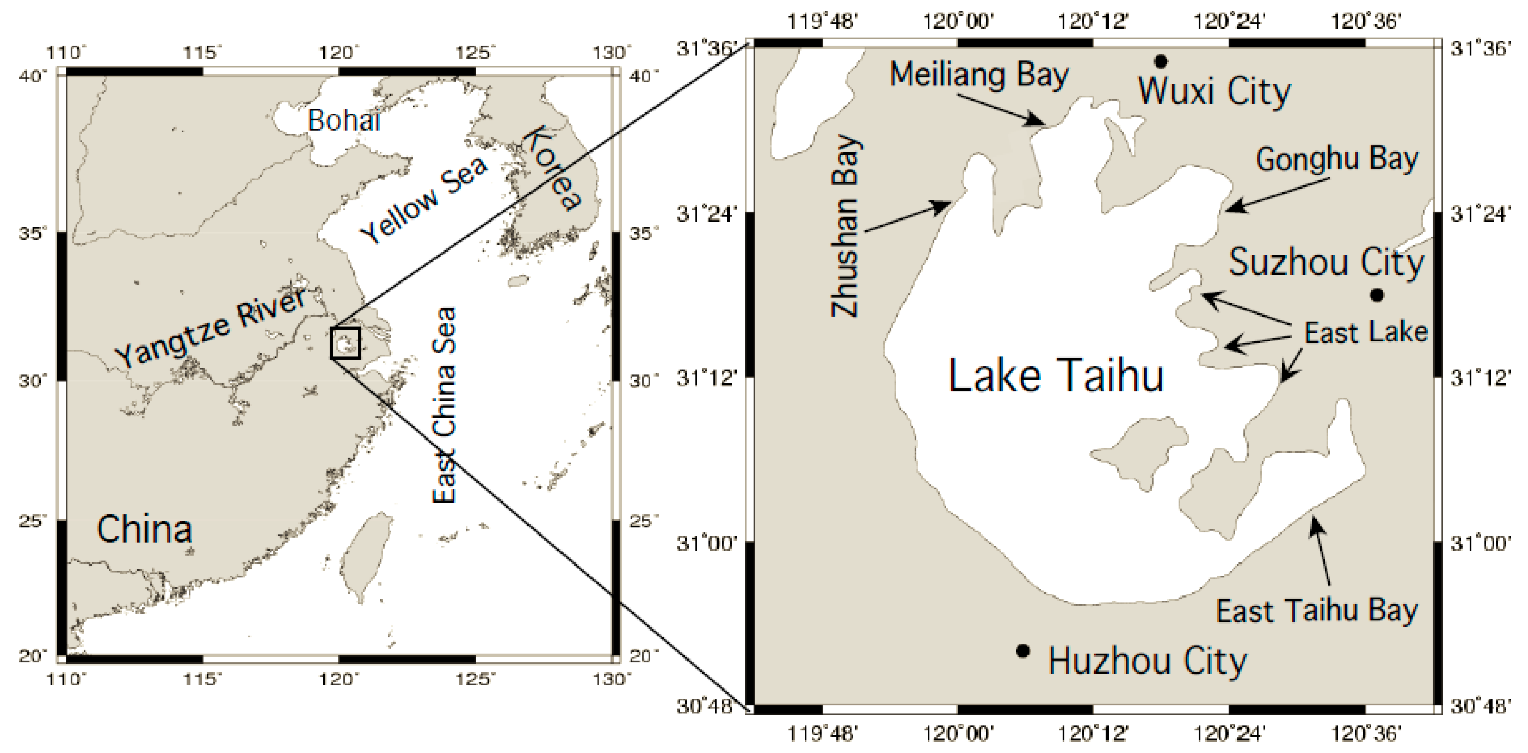
Lake Taihu is China’s third largest fresh water lake, and it is located in the Yangtze River Delta (Figure 1). It covers an area of ~2300 km2 with an average water depth of ~2 m. Lake Taihu features constantly turbid waters and frequent breakouts of algal blooms in the spring-summer. For example, a massive blue-green algae bloom broke out in the spring of 2007 and became an environmental crisis, which polluted the water supply for nearby urbanized and heavily populated regions [1,2,3].
Numerous studies have been conducted with both in situ measurements and satellite ocean color observations in order to develop satellite algorithms for geophysical and biological parameter retrievals, study the environmental changes, and to characterize and quantify the physical, biological, and biogeochemical dynamics, such as water quality, phytoplankton algal blooms, lake eutrophication, chlorophyll-a (Chl-a) concentration, water diffuse attenuation coefficient at the wavelength of 490 nm Kd(490) [4] or at the domain of photosynthetically available radiation (PAR) Kd(PAR) [5], primary production and color dissolved organic matters (CDOM), etc. Using the Moderate Resolution Imaging Spectroradiometer (MODIS) observations, Wang et al. [2] analyzed the massive blue-green algae bloom event during the spring of 2007, and derived the water properties for water quality monitoring, assessments, and management in Lake Taihu [2]. The intense blooms of cyanobacteria (primarily Microcystis aeruginosa) in Lake Taihu were also characterized with MODIS observations [6]. The annual frequency of significant blooms was found to increase from the time period of 2000–2004 to 2006–2008 [6]. The total suspended matter (TSM) concentration can also be retrieved and evaluated in Lake Taihu with satellite observations [7,8]. The long-term variability of the TSM concentration in Lake Taihu was characterized and quantified [7].
In recent years, the environment in Lake Taihu has been deteriorating significantly [9]. The water quality in northern Lake Taihu is getting worse due to urban pollutant discharge. The eutrophication in eastern Lake Taihu is caused by intensive aquaculture [9]. Climate variability and poor lake management are attributed to the crisis of the blue-green algal bloom in 2007. Similar to the lakes in the middle and low reaches of the Yangtze River, Lake Taihu also experienced eutrophication and the corresponding ecosystem responses, including the extinction of underwater plants and frequent cyanobacterial blooms [10]. The annual average total nitrogen concentration in Lake Taihu is ~2–3 mg L−1, and the phosphorus concentration is ~0.2 mg L−1, with significant spatial and temporal variations. The phytoplankton growth in Lake Taihu is controlled by nitrogen and phosphorus inputs, as well as by climatic factors [6,11].
In Lake Taihu, Chl-a concentration typically peaks in the summer and reaches its minimum in the winter. The maximum primary production usually occurs in the spring and summer seasons [12]. The CDOM shows the spatial and seasonal dynamics in Lake Taihu [13]. CDOM absorption is significantly higher in the winter than in the summer [14]. This is caused by the degradation and release of fixed carbon in the phytoplankton and the underwater vegetation [15]. The spectral slope for the exponential decrease of the CDOM absorption ag(λ) is ~0.015 nm−1 [16] with seasonal variations. The backscattering spectra from the blue to near-infrared (NIR) wavelengths in Lake Taihu are flat [17]. In fact, they are highly related to the TSM concentrations [7,17,18]. Shi et al. [7] show that TSM concentrations in Lake Taihu have significant spatial and temporal variability. Seasonal changes in the TSM concentration for all parts of Lake Taihu are in the range of 25–80 mg L−1. The TSM in southern Lake Taihu can reach over ~100 mg L−1 in the wintertime, while low TSM concentrations of ~20–30 mg L−1 are located in the northern parts of Lake Taihu, such as Meiliang Bay and Gonghu Bay [7].
The lake water inherent optical properties (IOPs) include the absorption and scattering of the pure water, color dissolved and detrital organic matter, and particles in the water column. These are the intrinsic optical properties, which determine the normalized water-leaving radiance spectra nLw(λ), that can be measured or retrieved from the in situ or satellite radiometry sensors [19,20,21,22]. In comparison to these nLw(λ) spectra, retrievals of biological and biogeochemical parameters such as Chl-a, TSM, Kd(490) and IOPs can provide comprehensive information about the constituents in the water column, and interaction between different constituents in order for researchers to better understand the ecosystem dynamics in both regional and global ocean waters [23,24].
For the global ocean, several algorithms were developed in order to retrieve IOPs, i.e., the particle backscattering coefficient bbp(λ), the absorption coefficient of the phytoplankton aph(λ), etc. In the Garver-Siegel-Maritorena (GSM) IOP algorithm [19,25], a nonlinear least-square scheme is used in order to best fit the modeled remote sensing reflectance Rrs(λ) with Rrs(λ) spectra from the satellite or in situ measurements. This IOP algorithm uses a fixed bbp(λ) power law slope η, and a constant exponential degradation slope S for the dissolved and detrital matters (adg(λ)). In the Quasi-Analytical Algorithm (QAA) [21], a couple of empirical formulae are used first to compute backscattering coefficients at a reference wavelength bbp(λ0) and the bbp(λ) power law slope η. Then total absorption at(λ) is further decomposed into aph(λ) and adg(λ) using the empirical formulae with at(410), at(443), as well as remote sensing reflectance beneath the surface rrs(λ) at the blue and green bands. On the other hand, the generalized IOP (GIOP) algorithm is a generic IOP algorithm, which allows the researcher to specify the modeling assumption for the IOP parameters, construct and develop new semi-analytical IOP algorithms, and tune into regional IOP algorithms [22].
These three IOP retrieval algorithms generally work well in the open ocean and less-turbid coastal and inland waters. However, significant errors with these three IOP algorithms can occur in turbid coastal and inland waters, such as Lake Taihu. Specifically, for the QAA algorithm, rrs(λ) in the blue and green bands are the major inputs to estimate the bbp(λ0) and bbp(λ) power law slope η. The saturation of the rrs(λ) in the visible bands over highly turbid waters shows that rrs(λ) loses its sensitivity to the change of bbp(λ) [26,27,28], thereby resulting in significant errors in coastal and inland turbid waters, such as those in Lake Taihu.
Satellite-measured nLw(λ) spectra at the red and NIR wavelengths are rarely used in the open ocean, since their values are close to 0. However, over turbid coastal and inland waters, nLw(λ) spectra feature enhanced nLw(λ) at the red and NIR wavelengths [2,28,29,30]. This spectral feature of the coastal and inland waters is caused by the strong water absorption at the red and NIR wavelengths [31,32], as well as a significant decrease of absorptions by CDOM at the red and NIR wavelengths and the near zero absorption of the phytoplankton at the NIR wavelengths [21,33]. Thus, nLw(λ) spectra at the red and NIR wavelengths can provide unique information to address the complexity of turbid coastal and inland waters, while the spectral features at the traditional blue and green wavelengths often fail. Over coastal and inland water regions, Chl-a [34], Kd(490) [4,35], TSM [7,36,37], the floating algae index [38] and normalized difference algae index [39], can all be produced using the optical measurements at the red and NIR wavelengths from the in situ and satellite observations. These products from the ocean color observations can be used to study the long-term environmental variability, characterize and quantify the coastal and lake ecosystems, evaluate the dynamics of the coastal environment, and monitor the natural hazards and environmental events.
In Lake Taihu, several studies were conducted in order to develop an improved algorithm to accurately retrieve the IOPs. By shifting the wavelength reference for bbp(λ0) from 551 nm or 640 nm to 701 nm in the QAA algorithm, the IOP retrievals in Lake Taihu are improved [40]. Another study shows an improved QAA algorithm with double-reference bands, and divides the entire Lake Taihu into two types of waters using the spectral slopes of remote sensing reflectance between 677 and 701 nm [41].
Even though these two algorithms showed some improvements in comparison with the QAA retrievals, they are in situ focused, and are not designed to be applied to the satellite observations in Lake Taihu.
Recent studies [42,43,44] show that the semi-analytical radiance model [20] can be simplified for the nLw(λ) at the NIR wavelengths because the sea water absorption aw(λ) is normally ~1–2 orders higher than the other IOP components at the NIR wavelengths. Consequently, the bbp(λ) spectra for all wavelengths between the short blue and NIR can be computed analytically from bbp(λ) values at the two NIR bands (745 and 862 nm) in coastal and inland turbid waters [42]. In comparison, the bbp(λ) spectra derived from other IOP algorithms, e.g., QAA [21], significantly underestimate the true bbp(λ) values. Shi and Wang [42] suggest that the NIR-based bbp(λ) retrievals in turbid coastal and inland waters can be extended to the second step of the QAA IOP algorithm to further derive other IOP components, i.e., decompose the total absorption at(λ) into phytoplankton absorption aph(λ) and absorption coefficient adg(λ) for the dissolved and detrital matters in the water column.
In this study, in situ IOP measurements in Lake Taihu are used to tune the NIR-based IOP algorithm for satellite ocean color observations from the Visible Infrared Imaging Radiometer Suite (VIIRS) onboard the Suomi National Polar-orbiting Partnership (SNPP). The performance of the IOP algorithm is evaluated and analyzed. This IOP algorithm is then applied to VIIRS observations between 2012 and 2018 to derive IOP bbp(λ), aph(λ), and adg(λ) products in Lake Taihu. Climatology, seasonal variability of bbp(λ), aph(λ), and adg(λ) are computed, characterized, and quantified. Time series of bbp(λ), aph(λ), and adg(λ) in Lake Taihu between 2012 and 2018 are also evaluated.
2. In Situ Data and VIIRS-SNPP Data
2.1. In Situ Measurements of Rrs(λ), aph(λ), and adg(λ)
During the period between 2006 and 2007, extensive in situ measurement campaigns were conducted by the Nanjing Institute of Geography and Limnology, Chinese Academy of Sciences. Five cruises were carried out in 7–9 January 2006, 29 July–1 August 2006, 12–15 October 2006, 7–9 January 2007, and 25–27 April 2007. In each cruise, 50 stations covering the entire Lake Taihu (Figure 1) were set up. The measurements included hyperspectral remote sensing reflectance for wavelengths between 350 and 1050 nm, Kd(PAR), TSM concentration, Chl-a, detrital particle absorption coefficient ad(λ), CDOM absorption coefficient ag(λ), and phytoplankton absorption coefficient aph(λ) between 300 and 750 nm. The absorption coefficient of dissolved and detrital matter adg(λ) is the sum of ad(λ) and ag(λ). It is noted that no bbp(λ) was measured in these experiments due to technical difficulties in measuring the backscattering coefficient in the turbid shallow waters.
The optical measurements and the water samples were taken at depths of 50 cm below the water surface. In situ remote sensing reflectance and PAR at each station were measured under low wind conditions between local time 8:30–16:30. At each station, an ASD field spectrometer (Analytical Devices, Inc., Boulder, CO, USA) was used to measure the downwelling irradiance and upwelling radiance. To reduce the radiance measurement error and increase the signal-to-noise ratio (SNR), the radiance was measured 10 times at each station. The downwelling irradiance and upwelling radiances are used to compute the remote sensing reflectance Rrs(λ). The protocols and the procedures to measure and compute the reflectance, PAR, Kd(PAR), and IOP properties are detailed in [35,45]. Note that nLw(λ) spectra and remote sensing reflectance just below the surface rrs(λ) can be directly converted from the remote sensing reflectance Rrs(λ) as shown in Appendix A.
The quantitative filter technique (QFT) was used to determine the detrital absorption coefficient ad(λ) and phytoplankton absorption coefficient aph(λ). Methanol was used to partition the absorption of detritus and phytoplankton. Water samples were first filtered through a 47-mm-diameter Whatman 0.70 μm GF/F filter, and then re-filtered through a 25-mm-diameter 0.22 μm Millipore filter to measure CDOM absorption ag(λ). The absorption coefficients of ad(λ) and aph(λ) were measured with a Shimadzu UV-2401PC UV-Vis spectrophotometer. Details of the measurement process were described by Zhang et al. [14].
In this study, these in situ measurements are used to tune and validate the NIR-based IOP algorithm for the VIIRS-SNPP observations, in order to develop a satellite-based IOP algorithm to retrieve the IOP properties from the VIIRS-derived nLw(λ) spectra for Lake Taihu. Assuming that the biogeochemical parameters that determine the spectra of IOPs, such as the particle size distribution, composition, texture, and refractive index, do not change with time, the in situ tuned IOP algorithm for the VIIRS-SNPP is still valid, even though these in situ measurements were taken prior to the SNPP launch in late 2011.
2.2. VIIRS-SNPP Satellite Observations
Launched on 28 October 2011, VIIRS-SNPP provides continuous observations of Earth’s atmosphere, land and ocean [46], similar to the data derived from the Moderate Resolution Imaging Spectroradiometer (MODIS) onboard the Aqua and Terra satellites [47]. The reflective solar bands in VIIRS for ocean color observations are similar to MODIS, in order to produce continued and consistent global ocean color products. Specifically, the nominal central wavelengths of the visible bands (M1–M5) for the VIIRS ocean color observations are 410, 443, 486, 551, and 671 nm, with a bandwidth of 20 nm and a spatial resolution of 750 m. The nominal central wavelengths for the two NIR bands (M6 and M7) are 745 and 862 nm, and the wavelengths for the three shortwave infrared (SWIR) bands (M8, M10, and M11) are 1238, 1601, and 2257 nm. The measurements at the NIR and SWIR bands are used to carry out an atmospheric correction in the satellite ocean color data processing [48,49,50].
As a key product suite derived from VIIRS, ocean color Environmental Data Records (EDR) are derived using the Multi-Sensor Level-1 to Level-2 (MSL12) ocean color data processing software package from Sensor Data Records (SDR) (or Level-1B) [51]. In particular, the SWIR-based and NIR-SWIR combined atmospheric correction algorithms are used in turbid coastal and inland waters in order to derive accurate nLw(λ) spectra from the short blue to the NIR wavelengths. A couple of studies have already shown that good quality nLw(λ) spectra can be achieved for both the open ocean and coastal regions from MODIS-Aqua, VIIRS-SNPP, etc. [2,49,52,53]. Previous studies have also shown that the SWIR-based atmospheric correction with MODIS can be used to drive nLw(λ) spectra with good accuracy in Lake Taihu [2,54]. Specifically, the mean ratios and standard deviations of nLw(λ) between the satellite retrievals and the in situ measurements are 1.074 ± 0.206 and 0.950 ± 0.153 at the wavelengths of 443 and 555 nm, respectively [2]. In this study, a total of 3813 VIIRS-SNPP granules over Lake Taihu between 2012 and 2018 are used to derive nLw(λ) spectra with the NIR-SWIR atmospheric correction in MSL12. These nLw(λ) spectra are further used to derive the IOPs using the NIR-based IOP algorithm.
3. The NIR-Based IOP Algorithm in Lake Taihu and Its Performance
3.1. The NIR-Based IOP Algorithm
To compute the IOPs using the nLw(λ) spectra from the VIIRS observations, it is critical to accurately estimate bbp(λ) in the first step. In QAA, the total absorption coefficients at(λ) at the reference green/red wavelengths are empirically estimated. The reference at(λ0) is then applied to the water-leaving reflectance model to calculate bbp(λ0) at the green/red wavelengths. Following the bbp(λ0) and the empirical power law slope η of bbp(λ) calculated from Rrs(λ) in the visible bands, bbp(λ) spectra are consequently estimated. The at(λ) spectra are then further derived from the surface remote-sensing reflectance model with the known bbp(λ).
Following the retrievals of the bbp(λ) and at(λ) spectra, these at(λ) spectra are further decomposed into the dissolved and detrital absorption coefficient adg(λ) and the phytoplankton absorption coefficient aph(λ) in the second step. Further details of the decomposition procedure are shown in Appendix A.
The aw(λ) spectrum shows aw(λ) is significantly enhanced at the NIR wavelengths [31]. Thus, aw(λ) is one to two orders higher than the absorption coefficients of the other constituents at the NIR wavelengths in turbid coastal and inland waters, i.e., aw(λ) >> aph(λ), ag(λ), and ad(λ). Thus, bb(λ)/[a(λ)+bb(λ)] can be approximated as
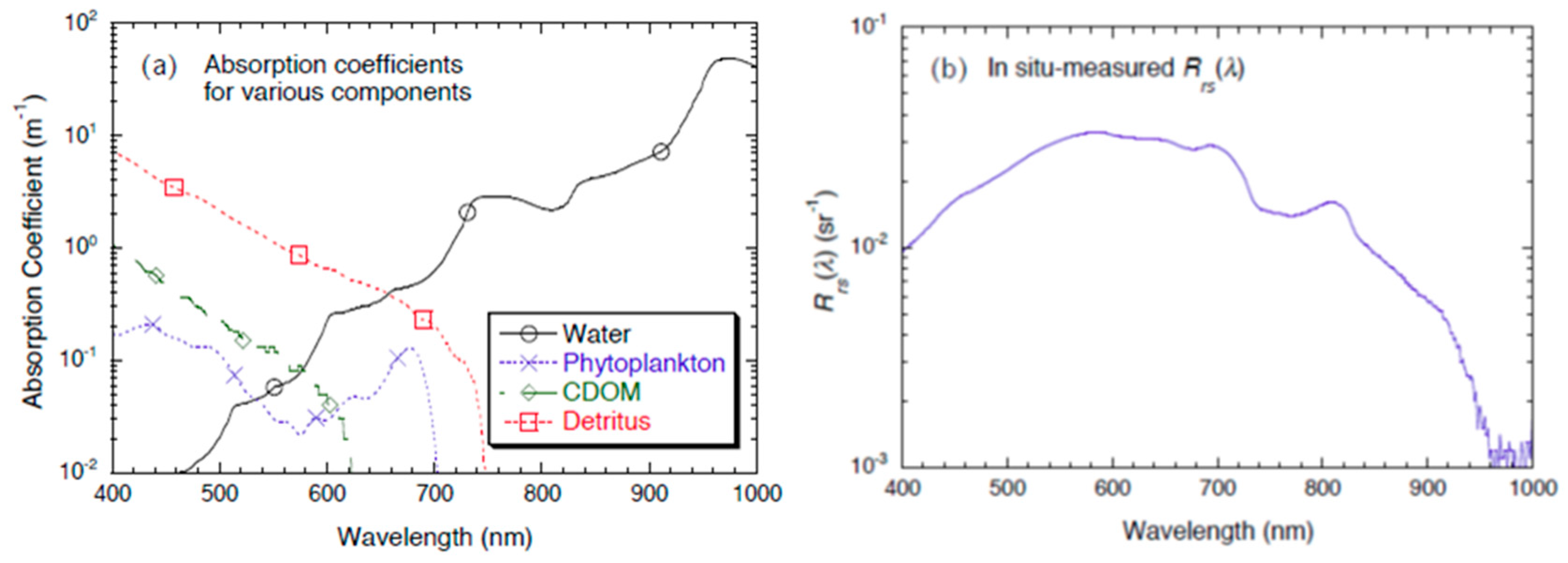
Figure 2a shows the in situ measurements of these aph(λ), ad(λ), and ag(λ) spectra in comparison with aw(λ) at [31.387°N, 120.267°E] measured on 7 January 2007, in Lake Taihu. The remote sensing reflectance Rrs(λ) spectrum (Figure 1b) peaks at the red wavelength, and the Rrs(λ) values are ~0.015 sr−1 and ~0.010 sr−1 at 745 and 862 nm, respectively. This suggests that Lake Taihu is a typical turbid inland lake. The aph(λ), ad(λ), and ag(λ) spectra at this station indeed show that aw(λ) at the NIR wavelengths is significantly higher than the other three IOP components, even though aph(λ), ad(λ), and ag(λ) are the dominant IOPs in the visible bands. Results in Figure 2a demonstrate that Equation 1 is a valid assumption for turbid coastal and inland waters. Thus, it can be used to derive the IOPs for coastal and inland waters.
In a recent study, Shi and Wang [42] demonstrated that the NIR-based bbp(λ) algorithm can be safely used for highly turbid waters with nLw(745) and nLw(862) < ~6 and 4 mW cm−2 μm−1 sr−1, respectively. In Lake Taihu, the MODIS and VIIRS observations show that nLw(859) or nLw(862) < ~2 mW cm−2 μm−1 sr−1 for all seasons [2,7]. This further shows that Equation 1 is valid for all seasons in Lake Taihu. Thus, this IOP algorithm can be applied to all VIIRS-SNPP observations between 2012 and 2018, in order to characterize and quantify the spatial and temporal IOP variations over Lake Taihu.
With this assumption, bbp(λ) at the two NIR bands can be analytically estimated, and the bbp(λ) power law slope η and bbp(λ) in the visible bands can be consequently calculated. In a recent study, Shi and Wang [42] demonstrated that bbp(λ) can be derived with good accuracy using the NIR-based backscattering algorithm and bbp(λ) data for global turbid coastal waters can be produced [42].
Following bbp(λ) retrievals in turbid coastal and inland waters like Lake Taihu, derived bbp(λ) data can be further extended to calculate at(λ) spectra with the remote-sensing reflectance model [20]. The other IOPs such as aph(λ) and adg(λ) are then further derived following a similar approach to step 2 of the QAA algorithm, i.e., to decompose at(λ) into aph(λ) and adg(λ). Note that the coefficients and formulae to decompose at(λ) into aph(λ) and adg(λ) in QAA are empirical, and default coefficients are tuned with in situ data for the global applications. IOP parameters such as the exponential decay slope S for adg(λ) can vary significantly from one region to another due to the difference of the particle size distribution, texture and composition, and particle refractive index [42]. As an example, the exponential decay slope S for adg(λ) can range from 0.008 to 0.018 [22]. Thus, it is necessary to re-tune it for Lake Taihu with the in situ IOP and nLw(λ) measurements, in order to optimize the coefficients and formulae in the second step in order to decompose at(λ) further into aph(λ) and adg(λ).
3.2. Performance of the NIR-Based IOP Algorithm in Lake Taihu
The default values in the quadratic equation for the remote sensing reflectance model in Gordon et al. [20] are 0.0949 for g1 and 0.0794 for g2 (see Appendix A). In this study, we optimize the retrievals of IOPs from the remote sensing reflectance in Lake Taihu by tuning g1 and g2 in order to obtain the best matches between retrieved at(λ) and the in situ at(λ) for VIIRS-SNPP application. We also use the in situ IOP and nLw(λ) measurements to recalculate the exponential decay slope S for adg(λ) as a function of nLw(410) and nLw(443) in Lake Taihu to further decompose at(λ) into aph(λ) and adg(λ) from VIIR-SNPP observations.
Following the procedure as described in Appendix A, we used the in situ measurements of adg(λ) and aph(λ) to tune the coefficients g1 and g2 of the quadratic formula in Gordon et al. (1988), so as to optimize the retrievals of at(λ) from the remote sensing reflectance in Lake Taihu. In this study, the values for the tuned g1 and g2 are 0.0626 and 0.0289, respectively.
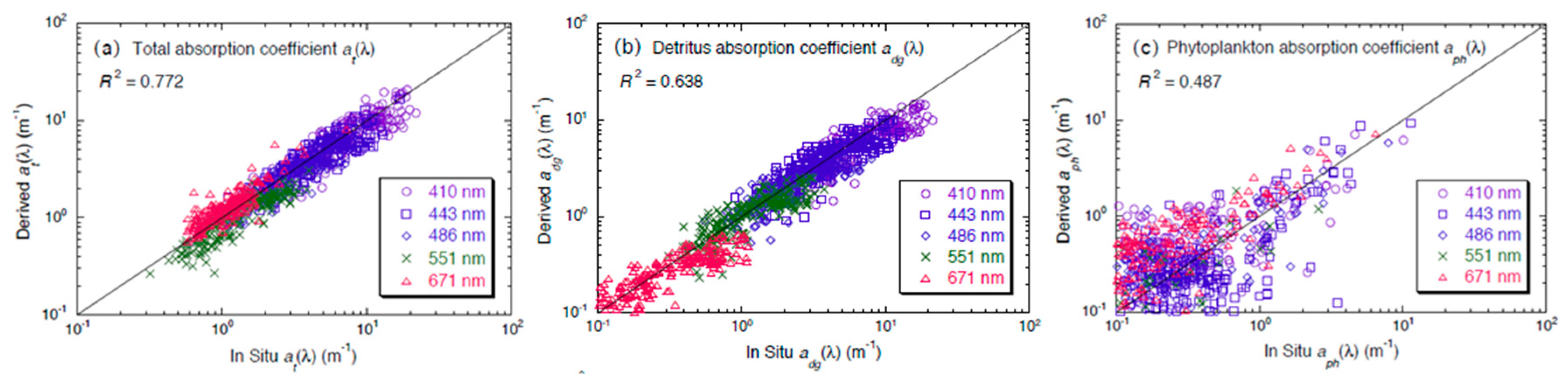
We also tune the coefficients and formulae to decompose the at(λ) into aph(λ) and adg(λ) using the in situ IOP and nLw(λ) data in Lake Taihu. It is found that the exponential slope S0 in Equation (A12) of Appendix A is set to 0.01056 in order to produce the best matches between the derived aph(λ) and adg(λ) using the in situ Rrs(λ) spectra and in situ aph(λ) and adg(λ) measurements. Details of the IOP algorithm for VIIRS-SNPP are described in Appendix A. Figure 3 shows the scatter plots of the derived IOP data versus the in situ IOP measurements for IOP parameters of at(λ) (Figure 3a), aph(λ) (Figure 3b), and adg(λ) (Figure 3c). In general, the in situ at(λ) measurements in Lake Taihu match well with at(λ) retrievals using the in situ Rrs(λ) spectra. The coefficient of determination R2 for these two at(λ) is 0.772 (Table 1). Table 1 also shows that these at(λ) retrievals have good performances for all the VIIRS bands with the best R2 of 0.810 for at(486).
The mean ratio of at(λ) between retrievals and the in situ at(λ) data is 0.970 ± 0.233 (Table 2). The ratios of at(λ) are also generally good at most of the VIIRS bands. The ratio of at(671) is 1.118 ± 0.276. The relatively high at(671) ratio and standard deviation (STD) can be attributed to the significantly small at(671) values in Lake Taihu. It is noted that there are no results for bbp(λ), because there are no in situ bbp(λ) data, due to the difficulty of the bbp(λ) measurement in turbid waters like Lake Taihu. Since the radiance model shows that bbp(λ) can be determined from at(λ) and Rrs(λ), the good match between retrievals and the in situ at(λ) data suggests that bbp(λ) retrievals from the IOP algorithm are expected to match the true bbp(λ) values.
Figure 3b shows the matchup (scatter plot) results for the IOP parameter adg(λ). The coefficient of determination for the match between the derived and in situ-measured aag(λ) data is 0.638 (Table 1). The mean adg(λ)/adgi(λ) for all the VIIRS bands are 0.948 ± 0.298. Table 1 and Table 2 also show that adg(λ) retrievals from the remote sensing reflectance have good accuracies for all of the VIIRS bands.
Lower accuracies and higher uncertainties can be found for aph(λ) retrievals even though fair comparison results are shown in the aph(λ) scatter plot between derived and in situ-measured aph(λ) data (Figure 3c). The coefficient of determination R2 for these two aph(λ) is 0.487 (Table 1), and the mean ratio of the derived/in situ in aph (λ) for all VIIRS bands is 1.196 ± 0.728 (Table 2). In comparison to the matchup plot of adg(λ) in Figure 3b, a large uncertainty can be found for aph(λ) retrievals, especially when aph(λ) is lower than ~1 m−1.
It is noted that the IOP retrievals show significant improvements in comparison to the un-tuned original IOP algorithm. The R2 values for the un-tuned IOP algorithm are 0.578, 0.302, and 0.251, while the IOP ratios are 1.02 ± 0.285, 0.56 ± 0.243, and 2.24 ± 1.19 for at(λ), adg(λ), and aph(λ), respectively. The IOP algorithm from Lee et al. [21] has a performance similar to the un-tuned original IOP algorithm. This suggests that it is necessary to tune the IOP algorithm in Lake Taihu in order to produce accurate IOP products for characterizing and quantifying the IOP dynamics in Lake Taihu, and the tuned IOP algorithm with g1 and g2 of 0.0626 and 0.0289, respectively, is optimal for Lake Taihu.
Even though there are no in situ measurements of bbp(λ) due to the technical difficulties, a conversion was also conducted to use the in situ Rrs(λ) spectra and at(λ) to further compute the corresponding bbp(λ) at the VIIRS bands using the tuned quadratic Equation (A3). As expected, the derived “in situ bbp(λ)” match well with the bbp(λ) retrievals at the corresponding VIIRS bands from the IOP algorithm. The coefficient of determination R2 for these two bbp(λ) is 0.779, and the IOP ratio of derived/in situ bbp(λ) is 1.010 ± 0.216.
The IOP in situ measurements for tuning the IOP algorithms were collected across Lake Taihu, and covered all four seasons. Thus, all variations of the parameters are related to the IOPs, such as particle size distribution, particle type, shapes, refractive index, a*ph(λ) spectral shapes, a*dg(λ) spectral shapes, etc., have already been included in this in situ dataset. Correspondingly, the IOP algorithm tuned with the in situ dataset should be insensitive to the changes of these IOP parameters. Consequently, the tuned IOP algorithm can be applied to the entire Lake Taihu and for all seasons to derive the IOP properties, in order to study the IOP spatial variability and temporal dynamics from the satellite observations. The IOP retrieval accuracy should be comparable to the IOP accuracy as described in Table 1 and Table 2.
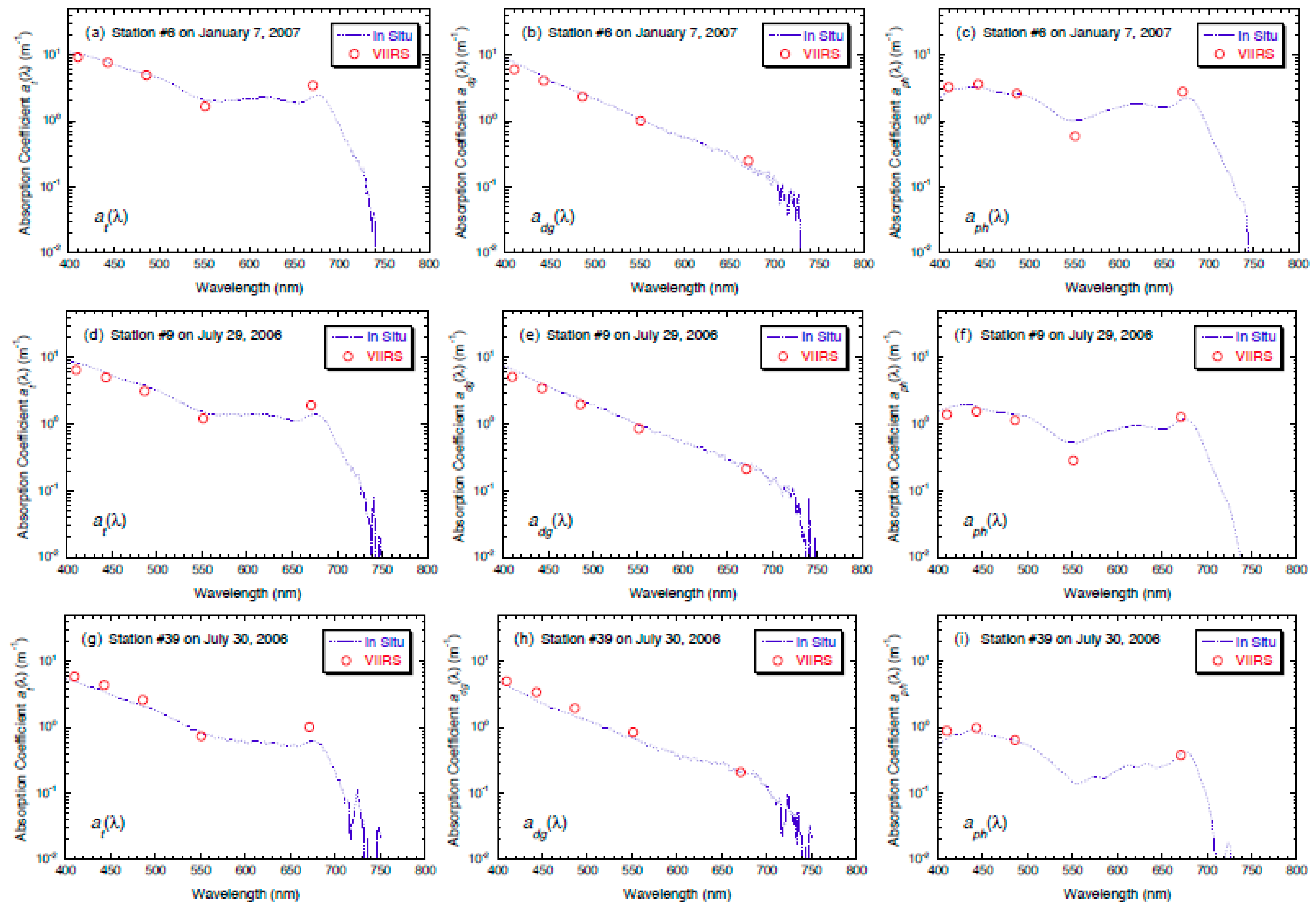
Retrievals of at(λ), adg(λ), and aph(λ) at the VIIRS bands are also compared with the corresponding in situ data at different stations. Figure 4 provides the examples of these comparisons at various measurement stations. At station #06 [31.504°N, 120.179°E] on 7 January 2007, retrieved at(λ) generally match the in situ at(λ) spectrum in the blue and green bands (Figure 4a). The curvature of the derived adg(λ) spectrum matches well with the in situ data (Figure 4b). Similarly, aph(λ) retrievals also show a good match with the in situ aph(λ) (Figure 4c).
Figure 4. shows at(λ), adg(λ), and aph(λ) retrievals in comparison with the corresponding in situ measurements at station #09 [31.506°N, 120.146°E] on 29 July 2006. The at(λ) retrievals generally match well with in situ at(λ), except that a notable underestimation in the derived at(λ) at the 410 nm band is observed (Figure 4d). Similarly, adg(λ) retrievals also show a good match with the in situ measurements (Figure 4e). The derived aph(λ) data are consistent with the aph(λ) measurements (Figure 4f). At station #39 on 30 July 2006, at(λ), adg(λ), and aph(λ) retrievals also show good matches with those from the in situ measurements (Figure 4g–i).
4. IOPs from VIIRS-SNPP Observations between 2012–2018
4.1. Climatology IOPs between 2012 and 2018
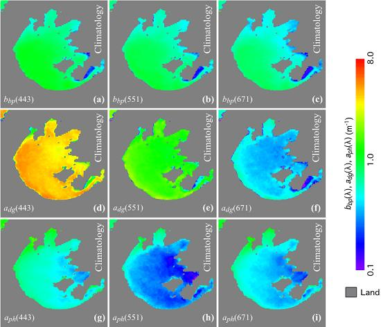
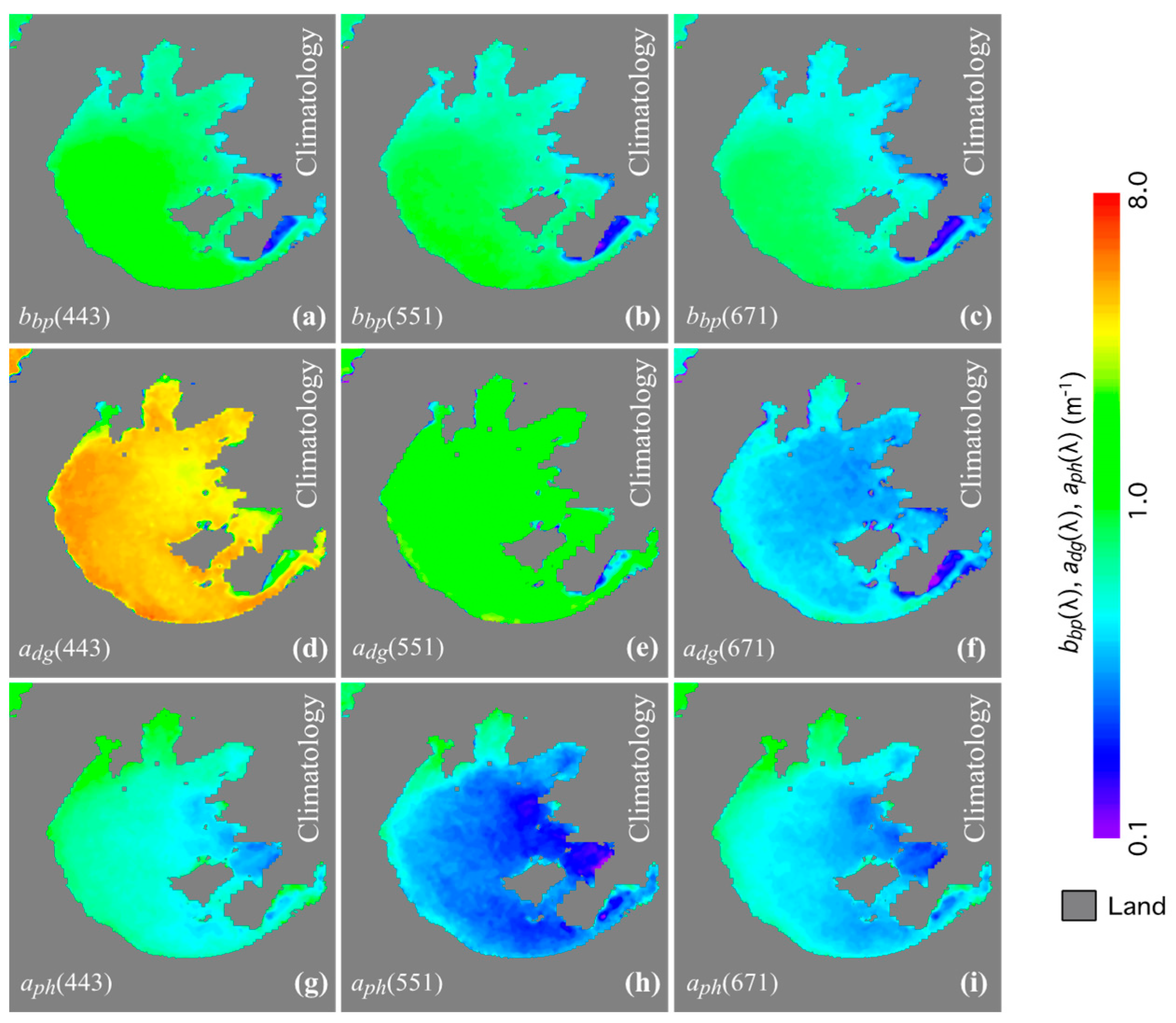
Figure 5 shows the VIIRS-SNPP-derived climatology bbp(λ) (Figure 5a–c), adg(λ) (Figure 5d–f), and aph(λ) (Figure 5g–i) at the bands 443, 551, and 671 nm from observations between 2012 and 2018. For each pixel, the climatology value is calculated as the median value of all the valid IOPs for this pixel from the VIIRS observations between 2012 and 2018. Of the three IOPs, aph(λ) is the lowest one in comparison with the corresponding bbp(λ) and adg(λ). In general, bbp(λ), adg(λ), and aph(λ) are not in phase with each other in terms of the spatial distributions and the spectral variations. At the bands 443 and 551 nm, adg(443) and adg(551) are the dominant IOPs in the three IOPs for most of Lake Taihu. At the VIIRS red band 671 nm, bbp(671) for Lake Taihu is generally larger than adg(671) and aph(671), except for northern Lake Taihu.
For bbp(λ), enhanced bbp(λ) can be found in southern and southwestern Lake Taihu, while relatively low bbp(λ) is found in the northern part of Lake Taihu. The spatial distribution of bbp(λ) is consistent with the TSM in Lake Taihu [7]. It is also noted that bbp(λ) slowly decreases spectrally from bbp(443) to bbp(671). In fact, this also suggests that the bbp(λ) spectral power law slope η is slightly positive and close to 0 [7].
The IOP parameter adg(λ) data are composed of ad(λ) from the non-algae detrital particles and ag(λ) from the dissolved matters. Lake Taihu is featured with enhanced adg(443), having values over ~4 m−1 in the eastern and southern regions of the lake. The adg(λ) decreases exponentially from adg(443) to adg(671). The spatial pattern of adg(λ) is not the same as the spatial pattern of bbp(λ) in Lake Taihu, even though both ad(λ) and bbp(λ) are proportional to the TSM concentration, i.e., TSM × specific ad*(λ) or bbp*(λ). Specifically, in Gonghu Bay, adg(λ) is significantly pronounced, while bbp(λ) in these regions are relatively low in comparison to those in southern Lake Taihu. This further implies that the ag(λ) in Meiliang Bay and Zhushan Bay are higher than those in the other parts of Lake Taihu.
In comparison to adg(λ) and bbp(λ), aph(λ) is usually low for most regions of Lake Taihu. However, pronounced aph(λ) can indeed be observed with aph(443) over ~1 m−1 in northern Lake Taihu, such as Meiliang Bay and Zhushan Bay, while no enhanced adg(443) is observed. The enhanced aph(443) is consistent with reports of algal blooms in those regions [55].
4.2. Seasonal Variability of IOPs in Lake Taihu
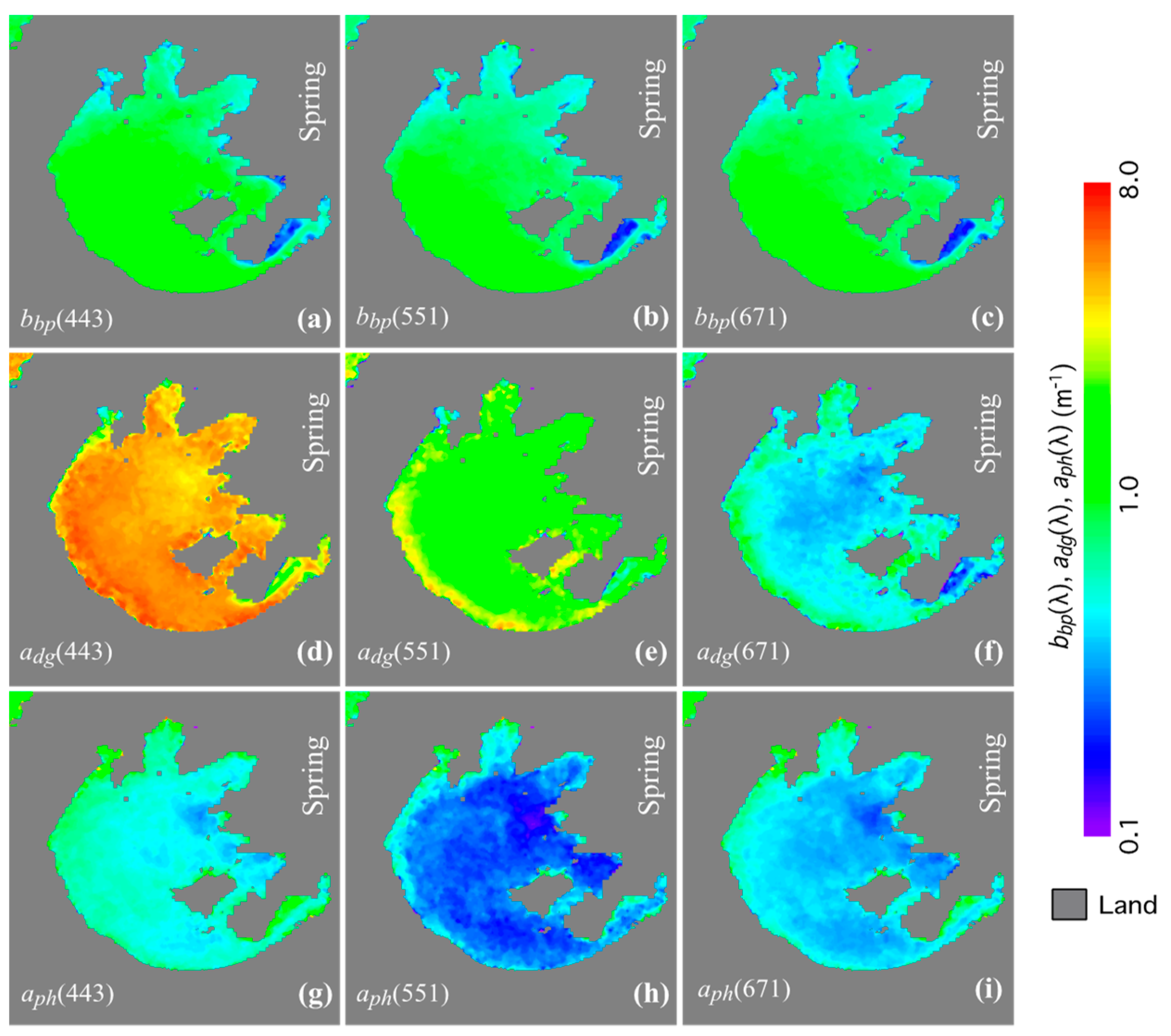
In Lake Taihu, seasonal variations of IOPs are significant. Figure 6 shows the bbp(λ), adg(λ), and aph(λ) in the spring season. Spatial distributions in bbp(λ) in the spring (Figure 6a–c) are similar to those of the climatology bbp(λ) with highs in southern Lake Taihu and lows in northern Lake Taihu. Enhanced adg(λ) (Figure 6d–f) can be found for the entire lake with adg(443) larger than ~4 m−1. In the near-shore region of Lake Taihu, Zhushan Bay, and Meiliang Bay, aph(443) can reach over ~1 m−1, while it is ~0.5 m−1 for most of Lake Taihu.
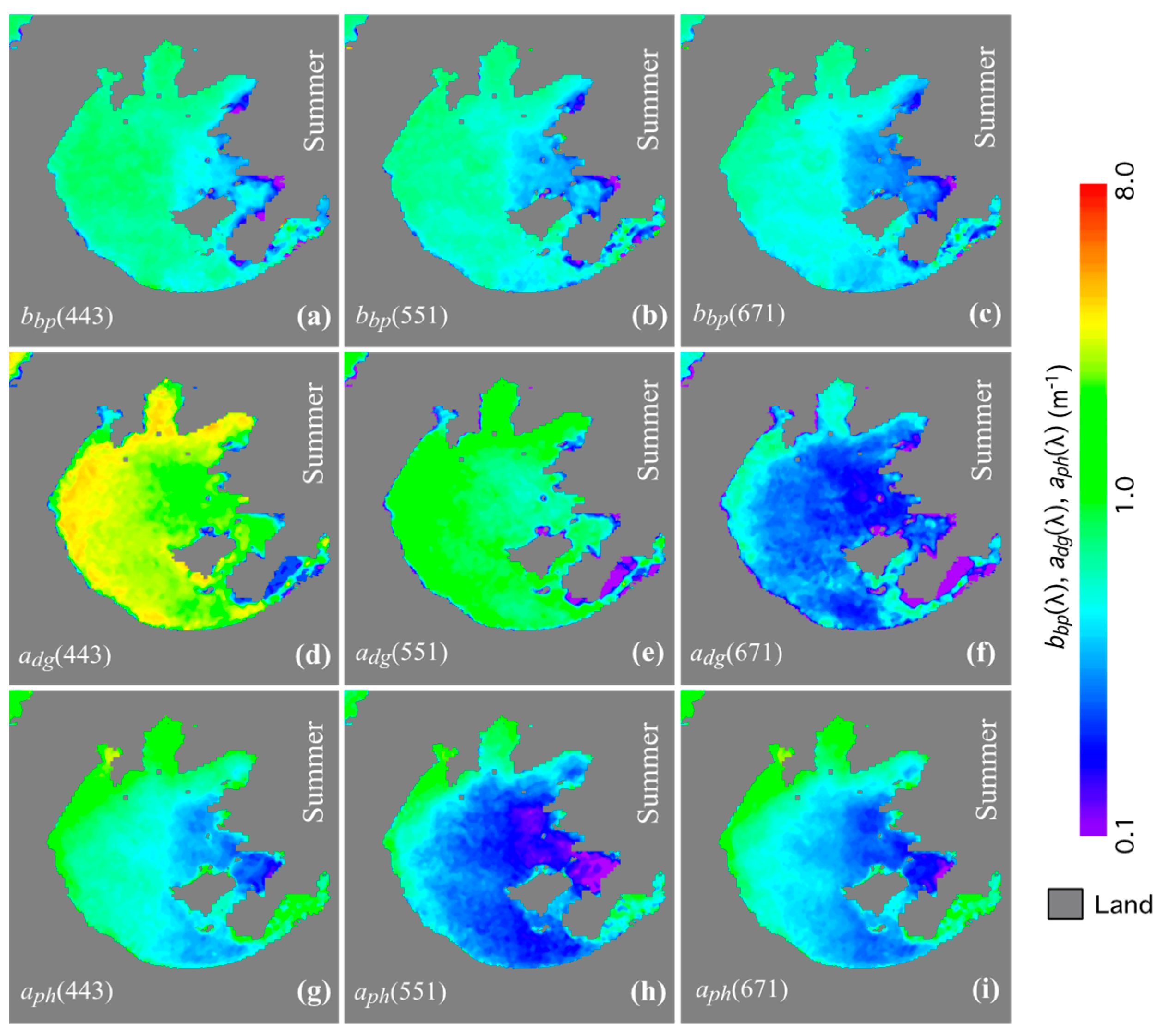
The summer season is the least turbid season in Lake Taihu, with the lowest bbp(λ) (Figure 7a–c). In the summer, adg(λ) also shows a significant drop in comparison with adg(λ) in the other seasons (Figure 7d–f). In fact, adg(443) in Lake Taihu is ~2–3 m−1, which is less than half of the adg(443) in the spring season. The values of aph(λ) in the summer are generally larger than those in the spring. Enhanced aph(λ) can also be found in the western coastal region and northern region of Lake Taihu.
It is noted that a large portion of the data noise in aph(λ) from a single observation can be filtered out when tens of aph(λ) observations are used to produce the seasonal IOPs. The previous study [12] also shows that a peak Chl-a occurs in the summer season. The in situ data from 2006–2007 in the lake show that the average aph(443) in the spring, summer, autumn, and winter were 1.22, 1.45, 0.95, and 0.34 m−1, respectively, while the corresponding VIIRS values from 2012–2018 are 0.65, 0.76, 0.59, and 0.46 m−1, respectively. The in situ mean adg(443) for the spring, summer, autumn, and winter were 3.12, 2.50, 2.77, and 6.92 m−1, respectively, compared with the corresponding VIIRS-derived mean adg(443) from 2012–2018 for these four seasons of 4.51, 2.14, 3.94, and 5.72 m−1. Thus, the seasonal variations in IOPs from the in situ data in Lake Taihu qualitatively agree with the IOP retrievals from VIIRS-SNPP measurements, and further demonstrate that aph(λ) and adg(λ) products from these VIIRS observations are reliable, and can be used to study the spatial and temporal dynamics of phytoplankton in Lake Taihu.
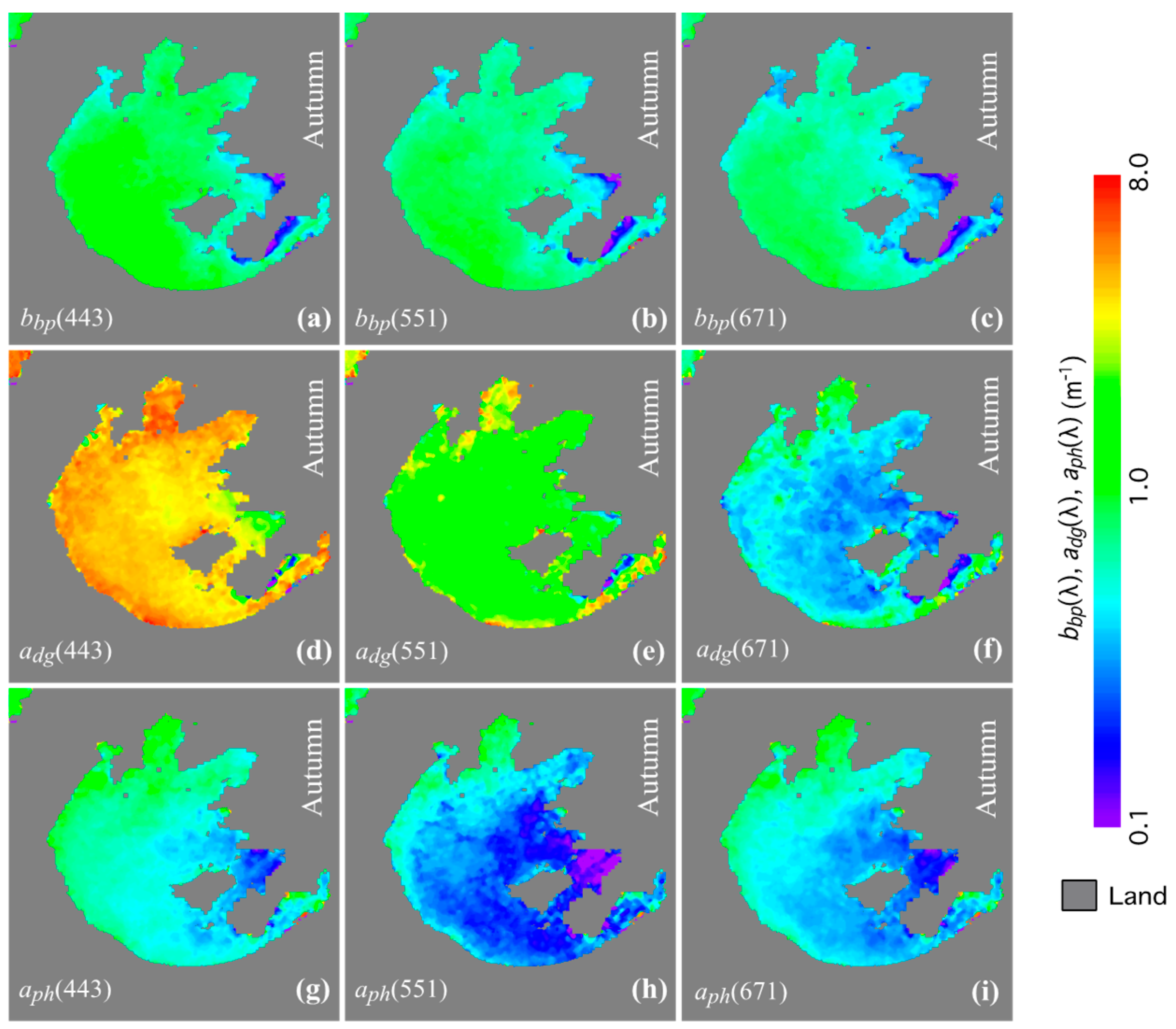
Figure 8 shows the IOP spatial distributions in the autumn season. A broad increase of bbp(λ) can be found in the autumn in comparison to the summer season (Figure 8a–c). Similarly, adg(λ) also shows significant increase in the summer (Figure 8d–f) with enhanced adg(λ) in the western coastal region and northern Lake Taihu. Also, it is noted that the spatial patterns of adg(λ) are not exactly the same as those of bbp(λ) in this and other seasons. This can be attributed to the contribution of ag(λ) in this season. In comparison to the changes of bbp(λ) and adg(λ) from the summer to autumn, the change of aph(λ) from the summer to autumn is less significant for most of Lake Taihu. In Zhushan Bay and Meiliang Bay, aph(λ) decreases from the summer to autumn.
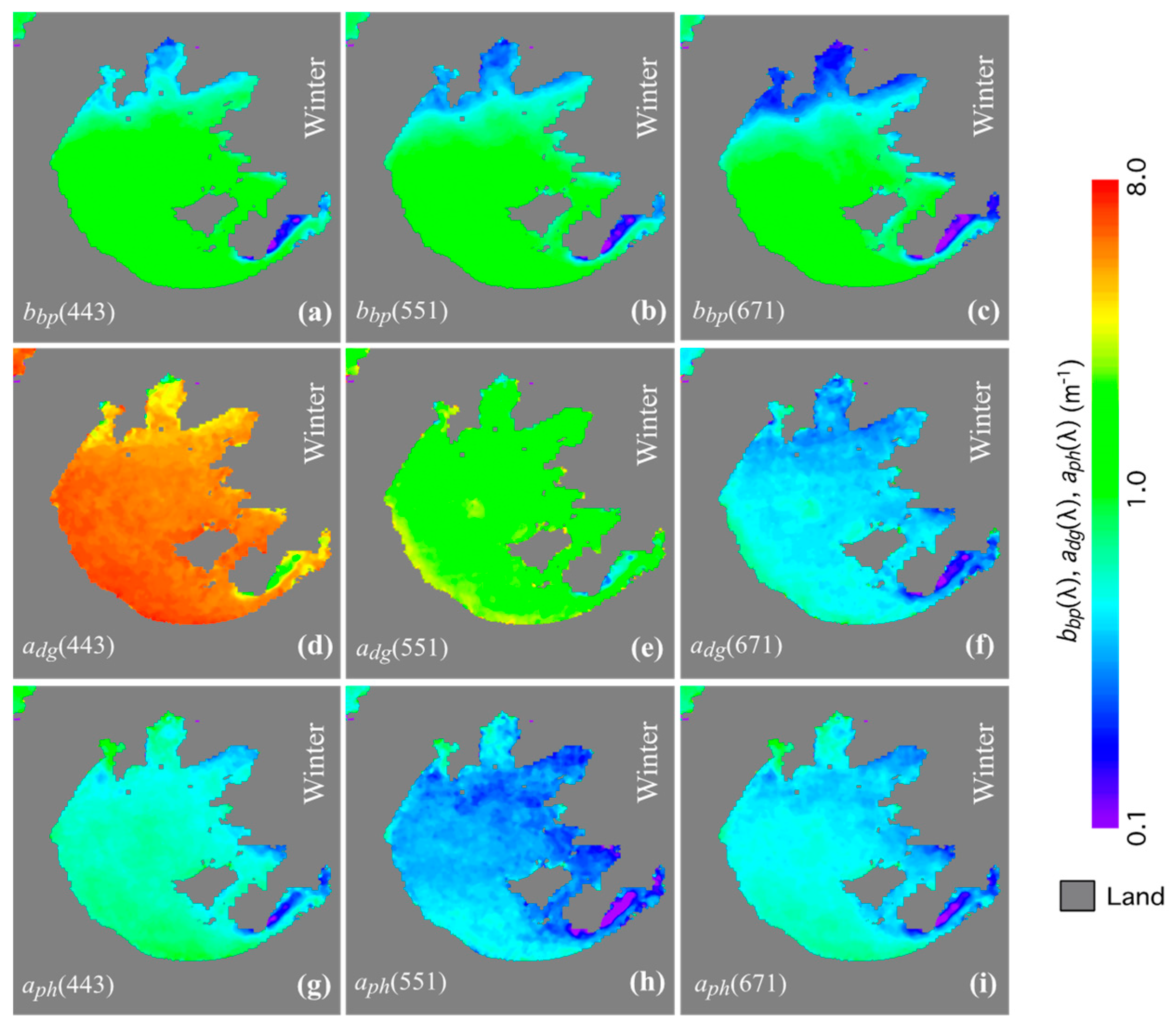
The highest bbp(λ) and adg(λ) can be found in the winter season (Figure 9a–f). In southern Lake Taihu, bbp(443) and adg(443) reach over ~1.5 m−1 and above 4–5 m−1, respectively. On the other hand, bbp(λ) is ~1 m−1, and adg(λ) is significantly smaller than the corresponding bbp(λ) in northern Lake Taihu. Furthermore, aph(λ) is flat for the entire Lake Taihu, and no enhanced aph(λ) can be found in northern Lake Taihu.
4.3. Time Series of IOPs in Lake Taihu between 2012 and 2018
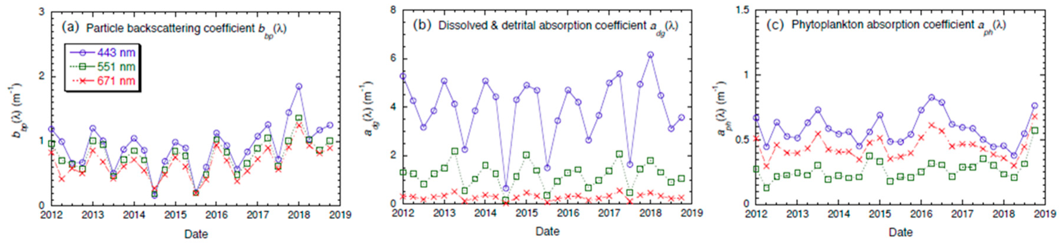
Figure 10 shows the IOP variations in Lake Taihu between 2012 and 2018. Of IOPs bbp(λ), adg(λ), and aph(λ), adg(λ) is the most prominent one. This is also evident in Figure 5, Figure 6, Figure 7, Figure 8 and Figure 9. Specifically, adg(443) is significantly larger than the corresponding bbp(443) and aph(443). In the seven-year period, bbp(λ) changed between ~0.3 and 2 m−1 with the notable seasonal variability. As shown in Figure 6, Figure 7, Figure 8 and Figure 9, the highest bbp(λ) occurred in the winter season and the lowest bbp(λ) in the summer season. Interannual variability was also significant in these seven years. In the summers of 2014 and 2015, the bbp(λ) was only ~0.3–0.4 m−1. The highest bbp(λ) occurred in the winter between 2017 and 2018 with bbp(443) over ~2 m−1 in Lake Taihu. Note that there is also an increasing trend for bbp(443) in the period of 2016–2018.
Overall, bbp(λ) and adg(λ) show similar seasonal and interannual trends in Lake Taihu (Figure 10b). In comparison to bbp(λ), adg(λ) shows more seasonal and interannual variabilities between 2012 and 2018. In the winter season, adg(443) reached over ~4 m−1, with the maximum adg(443) over ~6.0 m−1 in the winter between 2017 and 2018. The low adg(443) occurred in the summer season with adg(443) ~2.0 m−1 for most summers between 2012 and 2018. However, in the summer of 2014, adg(443) was only ~0.5 m−1.
In comparison to bbp(λ) and adg(λ), the phytoplankton absorption coefficient aph(λ) is the least significant IOP in terms of the magnitude and its contribution to the reflectance in the IOP model (Figure 10c). Seasonal and interannual variabilities in aph(λ) are not as significant as bbp(λ) and adg(λ), e.g., aph(443) ranging between 0.5 and 1.0 m−1. In the summer of 2013 and the spring-summer of 2016, aph(443) reached ~1.0 m−1. This suggests that the phytoplankton blooms in the summer of 2013 and the spring-summer of 2016 were more significant than in the other years.
5. Discussion
The nLw(λ) spectra in this study are derived using the SWIR-based atmospheric correction algorithm from the VIIRS observations. This is similar to the SWIR-based atmospheric correction algorithm for the MODIS observations [2]. In fact, the same MSL12 ocean color data processing system has been used in both studies. We examined the nLw(λ) climatology derived from VIIRS observations [7] and MODIS observations in Lake Taihu [2,28], and concluded that the climatology nLw(λ) spectra from these two studies are very close/similar in terms of both the magnitudes and the spatial patterns. This shows that VIIRS-derived nLw(λ) spectra are reliable, and can be used to produce the IOP products in Lake Taihu.
On the other hand, nLw(λ) bias in highly turbid waters may indeed occur in the blue band. It can reach up to ~0.5 mW cm−2 μm−1 sr−1 at the blue band for extremely turbid waters like Hangzhou Bay [27], and much less at the other bands. The water reflectance spectra in Lake Taihu [7,28] suggest that the winter is the only season when the low biased nLw(443) can occur. VIIRS-derived nLw(443) may be biased low ~ < 0.2 mW cm−2 μm−1 sr−1 with the SWIR-based atmosphere correction algorithm. The assessment of the nLw(λ) in Lake Taihu implies that there should be little bias for bbp(λ), at(λ), adg(λ), and aph(λ) in the spring, summer, and autumn seasons.
In the winter season, however, no or insignificant bias is expected for the bbp(λ) product since bbp(λ) is derived directly from nLw(λ) at the NIR wavelengths. However, VIIRS-derived at(443), adg(443), and aph(443) may be biased high, within ~10%.
It has long been a challenge to derive the IOP products from satellite ocean color observations in turbid coastal and inland waters. This challenge comes from two issues, i.e., an atmospheric correction for deriving accurate nLw(λ) spectra, and a valid IOP algorithm to retrieve IOPs in turbid coastal and inland waters. In the studies by Wang et al. [2,54], it has been shown that the SWIR-based atmospheric correction algorithm can be used to derive good quality nLw(λ) spectra from satellite observations. On the other hand, an NIR-based algorithm was proposed, developed, validated, and demonstrated to derive the backscattering coefficient bbp(λ) in turbid coastal and inland waters [42]. Based on the retrievals of bbp(λ) with the NIR-based algorithm, this study shows that the other IOPs such as adg(λ) and aph(λ) can also be subsequently retrieved after tuning and optimizing the coefficients in the procedure to decompose at(λ) into adg(λ) and aph(λ) with the in situ measurements. With the in situ IOP data, we developed the IOP algorithm in Lake Taihu from the VIIRS-SNPP observations. The comparison between IOP data derived from the NIR-based IOP algorithm and the in situ measurements shows that at(λ), adg(λ), and aph(λ) can be calculated with reasonable accuracy in Lake Taihu. A high determination coefficient between the derived at(λ) and in situ-measured at(λ) also suggests that bbp(λ) retrievals from the NIR-based IOP algorithm should also be reasonably accurate.
In this NIR-based IOP algorithm, the bbp(λ) spectral slope η is computed from bbp(745) and bbp(862), as shown in Equation A8 in Appendix A. Even though it is not an input/output parameter, η is critical in defining the spectral shapes of the IOPs and in determining the accuracy of the IOP retrievals. In Lake Taihu, the η calculated from the in situ Rrs(λ) range between −0.2 and 2.5 with the mean η of 1.13. Seasonal change of η is significant. Low η ~ 0 normally occurs in the winter season with enhanced Rrs(λ), while η is generally high in the summer and autumn seasons with low Rrs(λ). Examination of the VIIRS-SNPP observations also shows the similar seasonal variability in Lake Taihu.
The spatial patterns and temporal variations of the IOPs in Lake Taihu are driven by the physical and biogeochemical dynamics in Lake Taihu. In northern Lake Taihu, the enhanced aph(λ) in the summer and autumn seasons can be attributed to the frequent occurrence of the cyanobacterial blooms in that region [10]. In the spring and winter seasons, the enhanced bbp(λ) in southern and western Lake Taihu is consistent with the enhanced TSM concentrations caused by the sediment resuspensions due to high winds in these two seasons [7]. The spatial and temporal variations of adg(λ) in Lake Taihu are also driven by the physical and biogeochemical changes. The enhanced adg(λ) in the spring and winter seasons can be attributed to the high TSM in the water column [7] and degradation and release of fixed carbon in the phytoplankton and the underwater vegetation [15].
Both ad(λ) and bbp(λ) are proportional to the TSM concentration. Figure 5, Figure 6, Figure 7, Figure 8, Figure 9 and Figure 10 show that the changes of adg(λ) and bbp(λ) are different from each other. The main reason for the difference of the changes in adg(λ) and bbp(λ) is the role of ag(λ). In a turbid region like southern Lake Taihu, the ad(λ), which is proportional to the TSM concentration just like bbp(λ), is dominant in the adg(λ). However, in the less turbid waters of northern Lake Taihu, e.g., Meiliang Bay, ag(λ) is significantly enhanced due to a high CDOM centration from the phytoplankton decay. Thus, ag(λ) can be larger than ad(λ) in this region. This leads to the different changes in adg(λ) and bbp(λ).
It is also noted that no obvious seasonality of mean aph(λ) in the entire Lake Taihu shown in Figure 10c does not necessarily represent the regional aph(λ) seasonality in Lake Taihu. Figure 6, Figure 7, Figure 8 and Figure 9 clearly show that the northern and northwestern Lake Taihu regions experience notable seasonal variations of aph(λ). Enhanced aph(λ) can be observed in the summer-autumn seasons, while low aph(λ) occurs in the winter season. In the summer, aph(443) reaches over ~1.5 m−1, while aph(443) is generally below ~0.5 m−1 in the winter season.
Even though one of the purposes in this study is to develop the IOP algorithm for satellite observations in Lake Taihu, the approach for the regional NIR-based IOP algorithm can be further expanded to develop similar regional IOP algorithms for other coastal and inland water regions from a broad global perspective. On the other hand, the particles in Lake Taihu, the Yangtze River Estuary, and the Hangzhou Bay are all from the Yangtze River [56]. Thus, the nLw(λ) spectral shapes for these waters are similar [28]. Since the coefficients, such as the exponential decay coefficient S, are determined by the mineral type, composition, texture, particle refractive index, etc., this further implies that the particle type and composition for these waters are similar. Thus, the IOP algorithm for Lake Taihu in this study can be correspondingly applied to the other similar waters, such as the Yangtze River Estuary and Hangzhou Bay, in order to decompose at(λ) into adg(λ) and aph(λ) in those regions.
6. Conclusions
In this study, we applied the NIR-based IOP algorithm to VIIRS-SNPP observations to characterize and quantify the dynamics of the bbp(λ), adg(λ), and aph(λ) in Lake Taihu. In Lake Taihu, bbp(λ), adg(λ), and aph(λ) show significant spatial variability in the period between 2012 and 2018. The southern Lake Taihu region features enhanced bbp(λ) and adg(λ), while aph(λ) in northern Lake Taihu is significantly higher than those in the other regions. Of the three IOPs bbp(λ), adg(λ), and aph(λ), adg(λ) is the most significant IOP, while aph(λ) is the least one in terms of the IOP magnitude. Enhanced adg(λ) in northern Lake Taihu also implies that the CDOM absorption coefficient ag(λ) plays an important role.
This study also shows the significant temporal variability of bbp(λ) and adg(λ) in Lake Taihu in the period between 2012 and 2018. The highest bbp(λ) and adg(λ) occurred in the winter and the lowest bbp(λ) and adg(λ) occurred in the summer. In the winter, bbp(443) and adg(443) could reach over 1.5 and 5.0 m−1, respectively, while they are ~0.5–1.0 and ~2.0 m−1 in the summer. The highest bbp(λ) and adg(λ) occurred in the winter between 2017–2018, and the lowest bbp(λ) and adg(λ) occurred in the summer of 2014. In comparison to bbp(λ) and adg(λ), both the seasonal and interannual variations of aph(λ) are small.
Author Contributions
W.S. carried out the main research work for developing the algorithm, obtaining the results, and analyzing the data. M.W. suggested the topic, and contributed to the algorithm development. Y.Z. provided the in situ measurements, and helped validate the algorithm.
Funding
This work was supported by the Joint Polar Satellite System (JPSS) funding and NOAA Product Development, Readiness, and Application (PDRA)/Ocean Remote Sensing (ORS) Program funding. The collection of in situ data in Lake Taihu (Y. Zhang) was supported by the National Natural Science Foundation of China (Project Nos: 41621002, 41771472, and 41771514).
Acknowledgments
The VIIRS ocean color data and calibration/validation results can be found at the NOAA Ocean Color Team website (https://www.star.nesdis.noaa.gov/sod/mecb/color/) and VIIRS mission-long global ocean color data are freely available through the NOAA CoastWatch website (https://coastwatch.noaa.gov/). The views, opinions, and findings contained in this paper are those of the authors and should not be construed as an official NOAA or U.S. Government position, policy, or decision.
Conflicts of Interest
The authors declare no conflict of interest.
Appendix A
A NIR-Based IOP Algorithm for VIIRS-SNPP in Lake Taihu
The NIR-based IOP algorithm in Lake Taihu includes two steps. The first step is to derive the bbp(λ) and at(λ) spectra from the NIR to visible using nLw(λ) at the 745 and 862 nm bands. The second step is to decompose at(λ) into bbp(λ) and at(λ) following the procedure as shown in version 5 of the Quasi-Analytical Algorithm (QAA) [21], and tune the coefficients for Lake Taihu.
Step 1: Compute bbp(λ) and at(λ) from the VIIRS-SNPP nLw(λ)
Satellite-measured nLw(λ) product can be directly converted to the remote sensing reflectance in the IOP algorithm development, i.e.,
where nLw(λ) is the normalized water-leaving radiance and F0(λ) is the extraterrestrial solar irradiance. Above water remote sensing reflectance Rrs(λ) can be used to compute the subsurface remote sensing reflectance rrs(λ),
Rrs(λ) = nLw(λ)/F0(λ)
rrs(λ) = Rrs(λ)/(0.52 + 1.7 Rrs(λ))
In Gordon et al. [20], the subsurface remote sensing reflectance rrs(λ) is related to the IOPs as following,
where the original values in Gordon at al. [20] g1 = 0.0949 and g2 = 0.0794. These two values were computed from the in situ measurements. Coefficients a(λ) and bb(λ) are the total absorption at(λ) and backscattering coefficients, respectively. They are calculated as
where aw(λ), aph(λ), and adg(λ) are the absorption coefficients for the water, phytoplankton, and detrital and dissolve matters, respectively. bbw(λ) and bbp(λ) are the backscattering coefficients for the water and particles, respectively.
at(λ) = aw(λ) + aph(λ) + adg(λ)
bb(λ) = bbw(λ) + bbp(λ)
In the coastal and inland waters like Lake Taihu as shown in Figure 1 and demonstrated in Shi and Wang [42], the following assumption becomes valid at the NIR wavelengths, i.e.,
aw(λ) >> aph(λ), ag(λ), and ad(λ)
Following Equations (A3) and (A7), bbp(745) and bbp(862) are calculated from rrs(745) and rrs(862), then the bb(λ) power law slope η is calculated as a function of bbp(745) and bbp(862) as
After η is calculated, bbp(λ) is derived as
Consequently, at(λ) is calculated from the known bbp(λ) and rrs(λ) from Equation (A3). In this study, iterations with different combinations of g1 and g2 are applied to Equation 1 to derive the corresponding at(λ) from the in situ normalized water-leaving reflectance measurements. The deviation of the ratios between the retrieved at(λ) and in situ at(λ) is calculated with all available in situ Rrs(λ) and IOP measurements. The optimized g1 and g2 for Lake Taihu are selected as the pair with the ratio closest to 1.0. In this study, the values for the tuned g1 and g2 are 0.0626 and 0.0289, respectively. These two values are used as the regional IOP algorithm in Lake Taihu to derive the IOP properties from the VIIRS-SNPP observations.
Step 2: Decompose at(λ) into adg(λ) and aph(λ)
To decompose at(λ) into adg(λ) and aph(λ), ζ (aph(410)/aph(443)) is estimated with the empirical equation
Then, ξ (adg(410)/adg(443)) is assumed to follow the exponential decay function with coefficient S,
S is formulated as an empirical function of ,
The default of S0 is 0.015. In Lake Taihu, the in situ adg(λ) and show that the regionally optimized value of S0 is ~0.01056 nm−1. Thus, S0 is set to be 0.01056 nm−1 for the IOP algorithm in Lake Taihu.
After and are determined, adg(443) then can be calculated as:
Consequently, adg(λ), and aph(λ) are calculated with the following equations,
aph(λ) = at(λ) − adg(λ) − aw(λ).
References
- Guo, L. Ecology—Doing battle with the green monster of Taihu Lake. Science 2007, 317, 1166. [Google Scholar] [CrossRef] [PubMed]
- Wang, M.; Shi, W.; Tang, J.W. Water property monitoring and assessment for China’s inland Lake Taihu from MODIS-Aqua measurements. Remote Sens. Environ. 2011, 115, 841–854. [Google Scholar] [CrossRef]
- Qin, B.Q.; Zhu, G.W.; Gao, G.; Zhang, Y.L.; Li, W.; Paerl, H.W.; Carmichael, W.W. A drinking water crisis in Lake Taihu, China: Linkage to climatic variability and lake management. Environ. Manag. 2010, 45, 105–112. [Google Scholar] [CrossRef] [PubMed]
- Wang, M.; Son, S.; Harding, L.W. Retrieval of diffuse attenuation coefficient in the Chesapeake Bay and turbid ocean regions for satellite ocean color applications. J. Geophys. Res. Oceans 2009, 114. [Google Scholar] [CrossRef]
- Son, S.; Wang, M. Diffuse attenuation coefficient of the photosynthetically available radiation K-d(PAR) for global open ocean and coastal waters. Remote Sens. Environ. 2015, 159, 250–258. [Google Scholar] [CrossRef]
- Hu, C.M.; Lee, Z.P.; Ma, R.H.; Yu, K.; Li, D.Q.; Shang, S.L. Moderate Resolution Imaging Spectroradiometer (MODIS) observations of cyanobacteria blooms in Taihu Lake, China. J. Geophys. Res. Oceans 2010, 115. [Google Scholar] [CrossRef] [Green Version]
- Shi, W.; Zhang, Y.; Wang, M. Deriving total suspended matter concentration from the near-infrared-based inherent optical properties over turbid waters: A case study in Lake Taihu. Remote Sens. 2018, 10, 333. [Google Scholar] [CrossRef]
- Zhou, W.; Wang, S.; Zhou, Y.; Troy, A. Mapping the concentrations of total suspended matter in Lake Tailm, China, using Landsat-5 TM data. Int. J. Remote Sens. 2006, 27, 1177–1191. [Google Scholar] [CrossRef]
- Qin, B.Q.; Xu, P.Z.; Wu, Q.L.; Luo, L.C.; Zhang, Y.L. Environmental issues of Lake Taihu, China. Hydrobiologia 2007, 581, 3–14. [Google Scholar] [CrossRef]
- Zhu, M.Y.; Zhu, G.W.; Zhao, L.L.; Yao, X.; Zhang, Y.L.; Gao, G.; Qin, B.Q. Influence of algal bloom degradation on nutrient release at the sediment-water interface in Lake Taihu, China. Environ. Sci. Pollut. Res. 2013, 20, 1803–1811. [Google Scholar] [CrossRef]
- Xu, H.; Paerl, H.W.; Qin, B.Q.; Zhu, G.W.; Gao, G. Nitrogen and phosphorus inputs control phytoplankton growth in eutrophic Lake Taihu, China. Limnol. Oceanogr. 2010, 55, 420–432. [Google Scholar] [CrossRef]
- Zhang, Y.L.; Qin, B.Q.; Liu, M.L. Temporal—Spatial variations of chlorophyll a and primary production in Meiliang Bay, Lake Taihu, China from 1995 to 2003. J. Plankton Res. 2007, 29, 707–719. [Google Scholar] [CrossRef]
- Zhang, Y.L.; Yin, Y.; Liu, X.H.; Shi, Z.Q.; Feng, L.Q.; Liu, M.L.; Zhu, G.W.; Gong, Z.J.; Qin, B.Q. Spatial-seasonal dynamics of chromophoric dissolved organic matter in Lake Taihu, a large eutrophic, shallow lake in China. Org. Geochem. 2011, 42, 510–519. [Google Scholar] [CrossRef]
- Zhang, Y.L.; Zhang, B.; Wang, X.; Li, J.S.; Feng, S.; Zhao, Q.H.; Liu, M.L.; Qin, B.Q. A study of absorption characteristics of chromophoric dissolved organic matter and particles in Lake Taihu, China. Hydrobiologia 2007, 592, 105–120. [Google Scholar] [CrossRef]
- Zhang, Y.L.; van Dijk, M.A.; Liu, M.L.; Zhu, G.W.; Qin, B.Q. The contribution of phytoplankton degradation to chromophoric dissolved organic matter (CDOM) in eutrophic shallow lakes: Field and experimental evidence. Water Res. 2009, 43, 4685–4697. [Google Scholar] [CrossRef]
- Zhang, Y.L.; Qin, B.Q. Variations in spectral slope in lake taihu, a large subtropical shallow lake in China. J. Great Lakes Res. 2007, 33, 483–496. [Google Scholar] [CrossRef]
- Ma, R.H.; Pan, D.L.; Duan, H.T.; Song, Q.J. Absorption and scattering properties of water body in Taihu Lake, China: Backscattering. Int. J. Remote Sens. 2009, 30, 2321–2335. [Google Scholar] [CrossRef]
- Zhang, B.; Li, J.; Shen, Q.; Chen, D. A bio-optical model based method of estimating total suspended matter of Lake Taihu from near-infrared remote sensing reflectance. Environ. Monit. Assess. 2008, 145, 339–347. [Google Scholar] [CrossRef]
- Garver, S.A.; Siegel, D.A. Inherent optical property inversion of ocean color spectra and its biogeochemical interpretation.1. Time series from the Sargasso Sea. J. Geophys. Res. Oceans 1997, 102, 18607–18625. [Google Scholar] [CrossRef]
- Gordon, H.R.; Brown, O.B.; Evans, R.H.; Brown, J.W.; Smith, R.C.; Baker, K.S.; Clark, D.K. A semianalytic radiance model of ocean color. J. Geophys. Res. Atmos. 1988, 93, 10909–10924. [Google Scholar] [CrossRef]
- Lee, Z.P.; Carder, K.L.; Arnone, R.A. Deriving inherent optical properties from water color: A multiband quasi-analytical algorithm for optically deep waters. Appl. Opt. 2002, 41, 5755–5772. [Google Scholar] [CrossRef] [PubMed]
- Werdell, P.J.; Franz, B.A.; Bailey, S.W.; Feldman, G.C.; Boss, E.; Brando, V.E.; Dowell, M.; Hirata, T.; Lavender, S.J.; Lee, Z.P.; et al. Generalized ocean color inversion model for retrieving marine inherent optical properties. Appl. Opt. 2013, 52, 2019–2037. [Google Scholar] [CrossRef] [PubMed]
- Hu, C.M.; Lee, Z.P.; Muller-Karger, F.E.; Carder, K.L.; Walsh, J.J. Ocean color reveals phase shift between marine plants and yellow substance. IEEE Geosci. Remote Sens. Lett. 2006, 3, 262–266. [Google Scholar] [CrossRef]
- Siegel, D.A.; Maritorena, S.; Nelson, N.B.; Hansell, D.A.; Lorenzi-Kayser, M. Global distribution and dynamics of colored dissolved and detrital organic materials. J. Geophys. Res. Oceans 2002, 107. [Google Scholar] [CrossRef]
- Maritorena, S.; Siegel, D.A.; Peterson, A.R. Optimization of a semianalytical ocean color model for global-scale applications. Appl. Opt. 2002, 41, 2705–2714. [Google Scholar] [CrossRef]
- Shen, F.; Salama, M.S.; Zhou, Y.X.; Li, J.F.; Su, Z.B.; Kuang, D.B. Remote-sensing reflectance characteristics of highly turbid estuarine waters—A comparative experiment of the Yangtze River and the Yellow River. Int. J. Remote Sens. 2010, 31, 2639–2654. [Google Scholar] [CrossRef]
- Shi, W.; Wang, M. An assessment of the black ocean pixel assumption for MODIS SWIR bands. Remote Sens. Environ. 2009, 113, 1587–1597. [Google Scholar] [CrossRef]
- Shi, W.; Wang, M. Ocean reflectance spectra at the red, near-infrared, and shortwave infrared from highly turbid waters: A study in the Bohai Sea, Yellow Sea, and East China Sea. Limnol. Oceanogr. 2014, 59, 427–444. [Google Scholar] [CrossRef]
- Doron, M.; Belanger, S.; Doxaran, D.; Babin, M. Spectral variations in the near-infrared ocean reflectance. Remote Sens. Environ. 2011, 115, 1617–1631. [Google Scholar] [CrossRef]
- Ruddick, K.G.; De Cauwer, V.; Park, Y.J.; Moore, G. Seaborne measurements of near infrared water-leaving reflectance: The similarity spectrum for turbid waters. Limnol. Oceanogr. 2006, 51, 1167–1179. [Google Scholar] [CrossRef] [Green Version]
- Hale, G.M.; Querry, M.R. Optical constants of water in the 200 nm to 200 μm wavelength region. Appl. Opt. 1973, 12, 555–563. [Google Scholar] [CrossRef] [PubMed]
- Kou, L.H.; Labrie, D.; Chylek, P. Refractive-indexes of water and ice in the 0.65- to 2.5-μM spectral range. Appl. Opt. 1993, 32, 3531–3540. [Google Scholar] [CrossRef] [PubMed]
- Roesler, C.S.; Perry, M.J.; Carder, K.L. Modeling in situ phytoplankton absorption from total absorption-spectra in productive inland marine waters. Limnol. Oceanogr. 1989, 34, 1510–1523. [Google Scholar] [CrossRef]
- Gitelson, A.A.; Schalles, J.F.; Hladik, C.M. Remote chlorophyll-a retrieval in turbid, productive estuaries: Chesapeake Bay case study. Remote Sens. Environ. 2007, 109, 464–472. [Google Scholar] [CrossRef]
- Zhang, Y.; Liu, X.H.; Yin, Y.; Wang, M.Z.; Qin, B.Q. A simple optical model to estimate diffuse attenuation coefficient of photosynthetically active radiation in an extremely turbid lake from surface reflectance. Opt. Express 2012, 20, 20482–20493. [Google Scholar] [CrossRef] [PubMed]
- Miller, R.L.; McKee, B.A. Using MODIS Terra 250 m imagery to map concentrations of total suspended matter in coastal waters. Remote Sens. Environ. 2004, 93, 259–266. [Google Scholar] [CrossRef]
- Zhang, M.; Tang, J.W.; Dong, Q.; Song, Q.T.; Ding, J. Retrieval of total suspended matter concentration in the Yellow and East China Seas from MODIS imagery. Remote Sens. Environ. 2010, 114, 392–403. [Google Scholar] [CrossRef]
- Hu, C. A novel ocean color index to detect floating algae in the global oceans. Remote Sens. Environ. 2009, 113, 2118–2129. [Google Scholar] [CrossRef]
- Shi, W.; Wang, M. Green macroalgae blooms in the Yellow Sea during the spring and summer of 2008. J. Geophys. Res. Oceans 2009, 114. [Google Scholar] [CrossRef] [Green Version]
- Le, C.F.; Li, Y.M.; Zha, Y.; Sun, D.Y.; Yin, B. Validation of a quasi-analytical algorithm for highly turbid eutrophic water of Meiliang Bay in Taihu Lake, China. IEEE Trans. Geosci. Remote Sens. 2009, 47, 2492–2500. [Google Scholar]
- Pan, H.Z.; Lyu, H.; Wang, Y.N.; Jin, Q.; Wang, Q.; Li, Y.M.; Fu, Q.H. An improved approach to retrieve IOPs based on a quasi-analytical algorithm (QAA) for turbid eutrophic inland water. IEEE J. Sel. Top. Appl. Earth Obs. Remote Sens. 2015, 8, 5177–5189. [Google Scholar] [CrossRef]
- Shi, W.; Wang, M. Characterization of particle backscattering of global highly turbid waters from VIIRS ocean color observations. J. Geophys. Res. Oceans 2017, 122, 9255–9275. [Google Scholar] [CrossRef]
- Shi, W.; Wang, M. A blended inherent optical property algorithm for global satellite ocean color observations. Limnol. Oceanogr.: Methods 2009. [Google Scholar] [CrossRef]
- Shi, W.; Wang, M. Characterization of suspended particle size distribution in global highly turbid waters from VIIRS measurements. J. Geophys. Res. Oceans 2019, 124. [Google Scholar] [CrossRef]
- Zhang, Y.L.; Feng, L.Q.; Li, J.S.; Luo, L.C.; Yin, Y.; Liu, M.L.; Li, Y.L. Seasonal-spatial variation and remote sensing of phytoplankton absorption in Lake Taihu, a large eutrophic and shallow lake in China. J. Plankton Res. 2010, 32, 1023–1037. [Google Scholar] [CrossRef] [Green Version]
- Goldberg, M.D.; Kilcoyne, H.; Cikanek, H.; Mehta, A. Joint Polar Satellite System: The United States next generation civilian polar-orbiting environmental satellite system. J. Geophys. Res. Atmos. 2013, 118, 13463–13475. [Google Scholar] [CrossRef]
- Salomonson, V.V.; Barnes, W.L.; Maymon, P.W.; Montgomery, H.E.; Ostrow, H. MODIS—Advanced facility instrument for studies of the Earth as a system. IEEE Trans. Geosci. Remote Sens. 1989, 27, 145–153. [Google Scholar] [CrossRef]
- Gordon, H.R.; Wang, M. Retrieval of water-leaving radiance and aerosol optical-thickness over the oceans with SeaWiFS—A preliminary algorithm. Appl. Opt. 1994, 33, 443–452. [Google Scholar] [CrossRef]
- Wang, M.; Shi, W. The NIR-SWIR combined atmospheric correction approach for MODIS ocean color data processing. Opt. Express 2007, 15, 15722–15733. [Google Scholar] [CrossRef] [Green Version]
- Wang, M. Remote sensing of the ocean contributions from ultraviolet to near-infrared using the shortwave infrared bands: Simulations. Appl. Opt. 2007, 46, 1535–1547. [Google Scholar] [CrossRef]
- Wang, M.; Liu, X.; Tan, L.; Jiang, L.; Son, S.; Shi, W.; Rausch, K.; Voss, K. Impacts of VIIRS SDR performance on ocean color products. J. Geophys. Res. Atmos. 2013, 118, 10347–10360. [Google Scholar] [CrossRef]
- Wang, M.; Son, S.; Shi, W. Evaluation of MODIS SWIR and NIR-SWIR atmospheric correction algorithms using SeaBASS data. Remote Sens. Environ. 2009, 113, 635–644. [Google Scholar] [CrossRef]
- Barnes, M.; Cannizzaro, J.P.; English, D.C.; Hu, C. Validation of VIIRS and MODIS reflectance data in coastal and oceanic waters: An assessment of methods. Remote Sens. Environ. 2019, 220, 110–123. [Google Scholar] [CrossRef]
- Wang, M.; Son, S.; Zhang, Y.; Shi, W. Remote sensing of water optical property for China’s inland Lake Taihu using the SWIR atmospheric correction with 1640 and 2130 nm bands. IEEE J. Sel. Top. Appl. Earth Observ. Remote Sens. 2013, 6, 2505–2516. [Google Scholar] [CrossRef]
- Duan, H.T.; Ma, R.H.; Xu, X.F.; Kong, F.X.; Zhang, S.X.; Kong, W.J.; Hao, J.Y.; Shang, L.L. Two-Decade Reconstruction of Algal Blooms in China’s Lake Taihu. Environ. Sci. Technol. 2009, 43, 3522–3528. [Google Scholar] [CrossRef] [PubMed]
- Milliman, J.D.; Shen, H.T.; Yang, Z.S.; Meade, R.H. Transport and deposition of river sediment in the Changjiang estuary and adjacent continental-shelf. Cont. Shelf Res. 1985, 4, 37–45. [Google Scholar] [CrossRef]
Figure 1.
Maps of China’s inland Lake Taihu. The major regions in Lake Taihu are also marked.

Figure 2.
In situ measurements of (a) aph(λ), ad(λ), and ag(λ) and (b) remote sensing reflectance Rrs(λ) at the location [31.387°N, 120.267°E] measured at 13:10 PM local time on 7 January 2007 in Lake Taihu. The corresponding Chl-a and total suspended matter (TSM) were 14.5 mg m−3 and 90.30 g m−3, respectively.

Figure 3.
Comparisons of the near-infrared (NIR)-based inherent optical property (IOP) retrievals and in-situ measurements at the Visible Infrared Imaging Radiometer Suite (VIIRS) spectral bands for IOP of (a) at(λ), (b) adg(λ), and (c) aph(λ).
Figure 3.
Comparisons of the near-infrared (NIR)-based inherent optical property (IOP) retrievals and in-situ measurements at the Visible Infrared Imaging Radiometer Suite (VIIRS) spectral bands for IOP of (a) at(λ), (b) adg(λ), and (c) aph(λ).

Figure 4.
Spectra of the retrieved and in-situ at(λ), adg(λ), and aph(λ) for (a–c) at station #06 [31.504°N, 120.179°E] on 7 January 2007, (d–f) at station #09 [31.506°N, 120.146°E] on 29 July 2006, and (g–i) at station #39 [31.064°N, 120.036°E] on 30 July 2006.
Figure 4.
Spectra of the retrieved and in-situ at(λ), adg(λ), and aph(λ) for (a–c) at station #06 [31.504°N, 120.179°E] on 7 January 2007, (d–f) at station #09 [31.506°N, 120.146°E] on 29 July 2006, and (g–i) at station #39 [31.064°N, 120.036°E] on 30 July 2006.

Figure 5.
VIIRS-derived IOP climatology in Lake Taihu between 2012 and 2018 for (a–c) bbp(λ), (d–f) adg(λ), and (g–i) aph(λ) at the VIIRS bands of 443 nm (left column), 551 nm (middle column), and 671 nm (right column).
Figure 5.
VIIRS-derived IOP climatology in Lake Taihu between 2012 and 2018 for (a–c) bbp(λ), (d–f) adg(λ), and (g–i) aph(λ) at the VIIRS bands of 443 nm (left column), 551 nm (middle column), and 671 nm (right column).

Figure 6.
VIIRS-derived IOP in Lake Taihu during the spring season between 2012 and 2018 for (a–c) bbp(λ), (d–f) adg(λ), and (g–i) aph(λ) at the VIIRS bands of 443 nm (left column), 551 nm (middle column), and 671 nm (right column).
Figure 6.
VIIRS-derived IOP in Lake Taihu during the spring season between 2012 and 2018 for (a–c) bbp(λ), (d–f) adg(λ), and (g–i) aph(λ) at the VIIRS bands of 443 nm (left column), 551 nm (middle column), and 671 nm (right column).

Figure 7.
VIIRS-derived IOP in Lake Taihu during the summer season between 2012 and 2018 for (a–c) bbp(λ), (d–f) adg(λ), and (g–i) aph(λ) at the VIIRS bands of 443 nm (left column), 551 nm (middle column), and 671 nm (right column).
Figure 7.
VIIRS-derived IOP in Lake Taihu during the summer season between 2012 and 2018 for (a–c) bbp(λ), (d–f) adg(λ), and (g–i) aph(λ) at the VIIRS bands of 443 nm (left column), 551 nm (middle column), and 671 nm (right column).

Figure 8.
VIIR-derived IOP in Lake Taihu during the autumn season between 2012 and 2018 for (a–c) bbp(λ), (d–f) adg(λ), and (g–i) aph(λ) at the VIIRS bands of 443 nm (left column), 551 nm (middle column), and 671 nm (right column).
Figure 8.
VIIR-derived IOP in Lake Taihu during the autumn season between 2012 and 2018 for (a–c) bbp(λ), (d–f) adg(λ), and (g–i) aph(λ) at the VIIRS bands of 443 nm (left column), 551 nm (middle column), and 671 nm (right column).

Figure 9.
VIIRS-derived IOP in Lake Taihu during the winter season between 2012 and 2018 for (a–c) bbp(λ), (d–f) adg(λ), and (g–i) aph(λ) at the VIIRS bands of 443 nm (left column), 551 nm (middle column), and 671 nm (right column).
Figure 9.
VIIRS-derived IOP in Lake Taihu during the winter season between 2012 and 2018 for (a–c) bbp(λ), (d–f) adg(λ), and (g–i) aph(λ) at the VIIRS bands of 443 nm (left column), 551 nm (middle column), and 671 nm (right column).

Figure 10.
Time series of the mean IOP in Lake Taihu for (a) bbp(λ), (b) adg(λ), and (c) aph(λ) at the VIIRS bands of 443, 551, and 671 nm.
Figure 10.
Time series of the mean IOP in Lake Taihu for (a) bbp(λ), (b) adg(λ), and (c) aph(λ) at the VIIRS bands of 443, 551, and 671 nm.


Table 1.
Coefficients of determination R2 between the derived- and in-situ-IOPs in Lake Taihu.
| IOP | Coefficient of Determination R2 | |||||
|---|---|---|---|---|---|---|
| All Bands | 410 nm | 443 nm | 486 nm | 551 nm | 671 nm | |
| at(λ) | 0.772 | 0.760 | 0.810 | 0.784 | 0.745 | |
| adg(λ) | 0.681 | 0.656 | 0.662 | 0.523 | ||
| aph(λ) | 0.487 | 0.398 | 0.594 | 0.474 | 0.439 | 0.537 |
Table 2.
Statistics of the ratios with standard deviation (STD) values between the derived- and in-situ-IOPs in Lake Taihu.
Table 2.
Statistics of the ratios with standard deviation (STD) values between the derived- and in-situ-IOPs in Lake Taihu.
| IOP. | IOP Ratio of Derived/In Situ (Mean ± STD). | |||||
|---|---|---|---|---|---|---|
| All Bands | 410 nm | 443 nm | 486 nm | 551 nm | 671 nm | |
| at(λ) | 0.970 ± 0.233 | 0.975 ± 0.265 | 0.953 ± 0.238 | 0.905 ± 0.202 | 0.897 ± 0.186 | 1.118 + 0.276 |
| adg(λ) | .948 ± 0.298 | ± 0.273 | 1.001 ± 0.296 | 0.956 ± 0.297 | 0.943 ± 0.292 | 0.910 ± 0.331 |
| aph(λ) | 1.196 ± 0.728 | 1.272 ± 0.718 | 0.932 ± 0.641 | 0.967 ± 0.753 | 1.126 ± 0.891 | 1.683 ± 0.640 |
© 2019 by the authors. Licensee MDPI, Basel, Switzerland. This article is an open access article distributed under the terms and conditions of the Creative Commons Attribution (CC BY) license (http://creativecommons.org/licenses/by/4.0/).
Share and Cite
MDPI and ACS Style
Shi, W.; Wang, M.; Zhang, Y. Inherent Optical Properties in Lake Taihu Derived from VIIRS Satellite Observations. Remote Sens. 2019, 11, 1426. https://doi.org/10.3390/rs11121426
AMA Style
Shi W, Wang M, Zhang Y. Inherent Optical Properties in Lake Taihu Derived from VIIRS Satellite Observations. Remote Sensing. 2019; 11(12):1426. https://doi.org/10.3390/rs11121426
Chicago/Turabian StyleShi, Wei, Menghua Wang, and Yunlin Zhang. 2019. "Inherent Optical Properties in Lake Taihu Derived from VIIRS Satellite Observations" Remote Sensing 11, no. 12: 1426. https://doi.org/10.3390/rs11121426
Note that from the first issue of 2016, this journal uses article numbers instead of page numbers. See further details here.