A New Empirical Model of NmF2 Based on CHAMP, GRACE, and COSMIC Radio Occultation

1
Institute of Meteorology and Oceanography, National University of Defense Technology, Nanjing 211101, China
2
State Key Laboratory of Space Weather, Chinese Academy of Sciences, Beijing 100190, China
3
Institute of Communications and Navigation, German Aerospace Center, Kalkhorstweg 53, 17235 Neustrelitz, Germany
4
State Key Laboratory of Astronautic Dynamics, Xi’an Satellite Control Center, Xi’an 710043, China
*
Author to whom correspondence should be addressed.
Remote Sens. 2019, 11(11), 1386; https://doi.org/10.3390/rs11111386
Submission received: 8 March 2019
/
Revised: 21 May 2019
/
Accepted: 21 May 2019
/
Published: 11 June 2019
(This article belongs to the Special Issue Latest Results and Developments in GNSS Ionosphere Theory, Methods, Technologies, Applications and Future Challenges)
Abstract
:To facilitate F2-layer peak density (NmF2) modeling, a nonlinear polynomial model approach based on global NmF2 observational data from ionospheric radio occultation (IRO) measurements onboard the CHAMP, GRACE, and COSMIC satellites, is presented in this paper. We divided the globe into 63 slices from 80°S to 80°N according to geomagnetic latitude. A Nonlinear Polynomial Peak Density Model (NPPDM) was constructed by a multivariable least squares fitting to NmF2 measurements in each latitude slice and the dependencies of NmF2 on solar activity, geographical longitude, universal time, and day of year were described. The model was designed for quiet and moderate geomagnetic conditions (Ap ≤ 32). Using independent radio occultation data, quantitative analysis was made. The correlation coefficients between NPPDM predictions and IRO data were 0.91 in 2002 and 0.82 in 2005. The results show that NPPDM performs better than IRI2016 and Neustrelitz Peak Density Model (NPDM) under low solar activity, while it undergoes performance degradation under high solar activity. Using data from twelve ionosonde stations, the accuracy of NPPDM was found to be better than that of NPDM and comparable to that of IRI2016. Additionally, NPPDM can well simulate the variations and distributions of NmF2 and describe some ionospheric features, including the equatorial ionization anomaly, the mid-latitude trough, and the wavenumber-four longitudinal structure.
1. Introduction
The ionosphere is composed of several layers, namely the D-layer (50–90 km), E-layer (90–140 km), F1-layer (140–210 km), and F2-layer (210–1000 km) [1]. Among these layers, the F2-layer is the most ionized region, having the highest electron density variability. Therefore, the F2-layer is primarily responsible for most of the ionospheric effects, such as signal delay and ray path bending. The F2-layer peak electron density (NmF2) is one of the most important parameters to characterize the ionosphere. It is linearly related to the square of the critical frequency (foF2) of radio wave propagation. The variation of foF2 can result in the interruption or even loss of high frequency signal transmissions. In addition, the research on NmF2 is beneficial to reducing the influence of ionospheric propagation delay on global positioning. Thus, the performance of an NmF2 model is of great significance for ionospheric research and global navigation applications.
NmF2 may vary from about 1010 to 1013 m−3 during the daytime and decrease during nighttime [2]. The peak density height (hmF2) may range from 350 to 500 km at the equatorial latitudes and from 250 to 350 km at mid-latitudes. The variation of NmF2 is mainly affected by local time, season, sunspot numbers, geographical location, and solar disturbances.
To develop new NmF2 models or improve the existing models, researchers have conducted some interesting studies [3,4,5,6,7,8,9]. The International Reference Ionosphere (IRI) [6] and NeQuick model [10,11] are amongst the widely used empirical models. IRI uses CCIR (International Radio Consultative Committee) coefficients [12] and URSI (International Union of Radio Science) coefficients [13] to predict foF2. The CCIR and URSI coefficients were obtained from observations from the existing worldwide network of ionospheric sounding stations. Araujo-Pradere et al. [14] developed an NmF2 model for geomagnetic storms periods. Oyeyemi and McKinnell [15] built an foF2 model that can be used as a replacement for the CCIR and URSI coefficients within the IRI model. Many authors have used empirical orthogonal functions (EOF) to develop models for ionosphere parameter predictions and verified their results [16,17,18]. A new approach based on the neural network method was also tested for the modeling of foF2 [19,20,21,22,23]. The results showed that it was possible to forecast foF2 in near-real time (5 h in advance) by using this method. Recently, Sai and Tulasi [24] developed the Artificial Neural Network-Based Ionospheric Model (ANNIM) based on COSMIC (Constellation Observing System for Meteorology, Ionosphere and Climate) data to predict NmF2. They used the artificial neural network (ANN) method, a machine learning technique that is capable of solving highly nonlinear problems by systematic learning mechanisms. Tulasi et al. [25] then presented an improved version of ANNIM by including CHAMP (Challenging Minisatellite Payload) and GRACE (Gravity Recovery And Climate Experiment) IRO measurements as well as ionosonde data as data sources. They assessed the performance of the ANNIM by comparing it with the IRI-2016 model, and also showed that the ANNIM well reproduced the spatial and temporal variations of NmF2 and captured the ionospheric anomalies such as the equatorial ionosphere anomaly (EIA) and the mid-latitude summer night-time anomaly (MSNA). Themens et al. [26] used Fourier expansions and a spherical cap harmonic expansion for the quiet time NmF2 model and just a spherical cap harmonic expansion for the perturbed time NmF2 model based on ionosonde and IRO measurements. These models provided NmF2 predictions for a region above 50°N geomagnetic latitude. They demonstrated that their model provided improvements over IRI and was capable of representing auroral enhancements and the midlatitude trough.
Hoque and Jakowski [27] made an inspiring and successful attempt to develop a nonlinear model (Neustrelitz Peak Density Model—NPDM) with only 13 coefficients and a few empirically fixed parameters, which described the dependencies of NmF2 on local time, geographic/geomagnetic location, and solar irradiance and activity. The NPDM was proved to be a very efficient model with reasonable performance.
In this study, a nonlinear polynomial model approach was also used to develop the Nonlinear Polynomial Peak Density Model (NPPDM). We used the data of ionospheric radio occultation (IRO) measurements as the database, which included CHAMP, GRACE, and COSMIC observations. The model was based on a set of non-linear equations. Unlike the NPDM model, NPPDM included the longitudinal variation of NmF2. Other input variables were latitude, solar activity, day of year, and universal time. The latitudinal dependence of NmF2 was not described by an independent equation in our model. We divided the globe into 63 slices according to the geomagnetic latitude. The coefficients were derived in each slice from a multivariable fit to NmF2 measurements in least squares sense. To evaluate the fitting quality, the residuals of NPPDM were analyzed. Independent observations from IRO and twelve ionosonde stations worldwide were used for accuracy comparisons between NPPDM, IRI2016, and NPDM. In addition, some features of the spatial and temporal variations of NmF2 were simulated by NPPDM for further validations.
2. Data
The IRO technique has the advantages of limb sounding geometry, global coverage, and high vertical resolution in comparison with traditional ionosphere monitoring methods. Under certain assumptions, the total electron content (TEC) derived from the dual-frequency observations along the GPS ray can be inverted to the electron density profile (EDP) assigned to the tangent points of the rays by a traditional Abel inversion [28,29]. Investigations by several authors [30,31] showed that accurate hmF2 and NmF2 of the F2-layer can be obtained from occultation observations through the Abel transformation. The studies of Lei et al. [32], Angling [33], and Krankowski et al. [34] showed that the NmF2 and hmF2 derived from IRO technique are consistent with the observations of ionosonde and incoherent scatter radar. It should be noted that although the retrieved NmF2 by IRO techniques are generally in good agreement with ionosonde observations at middle latitudes [30,35], the accuracy of the Abel inverted electron density degrades at low latitudes, especially at the EIA region. The NmF2 inversion error in the EIA region is characterized by overestimation in the trough region and underestimation in the crest region due to the smoothing operation during the retrieval process. The relative error of NmF2 could account for up to 20%, with most amplitudes within ±10% [30].
In this study, the peak electron densities of EDPs were used as the database for NmF2 modeling. The EDPs from CHAMP and GRACE were provided by the German Aerospace Center (DLR) Neustrelitz (http://swaciweb.dlr.de/). The EDPs from COSMIC were processed by COSMIC Data Analysis and Archive Center (CDAAC, http://cosmic-io.cosmic.ucar.edu/cdaac/index.html). We selected profiles that satisfied the following criteria: (1) The daily geomagnetic activity index (Ap) was less than 32 to avoid the disturbed NmF2 due to geomagnetic storm events; (2) Observations in the polar regions (80°–90° N/S) were removed due to data deficiency; (3) A least-squares fitting to a two-layer Chapman function was performed to each EDP [36]:
We set the Chapman scale height as for the bottomside and for the topside. Here, is the value of at hmF2, while and are coefficients.
After the fitting, the same criteria proposed by Yue et al. [36] was used: if the fitted NmF2 (larger than 107/cm3), hmF2 (higher than 600 km or lower than 150 km), Hm (larger than 150 km) values were unreasonable or the difference between the fitted NmF2/hmF2 and that derived from the EDP directly by taking the maximum of the profile was larger than 20%, the EDP will be discarded. This procedure will ensure the integrity of the results in the study because those outliners might mean something wrong in the profile observation or processing. The final details of the selected database are listed in Table 1.
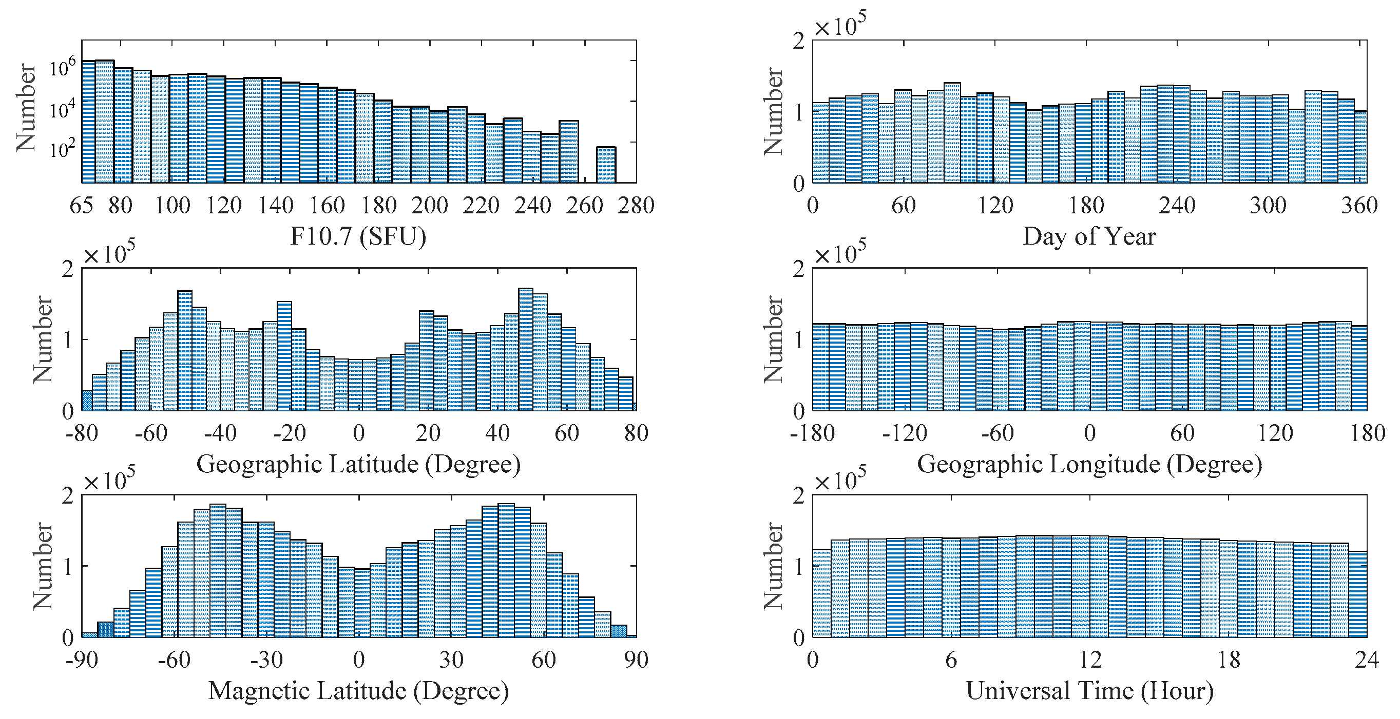
Distributions of the database with the solar activity (F10.7 index), day of year, geographical latitude, geographical longitude, magnetic latitude, and universal time are shown in Figure 1. From Figure 1, it can be clearly seen that most of the data are distributed in mid and low latitudes and few are distributed in high latitudes. Similarly, the data under low solar activity are in the majority compared with that under high solar activity.
Moreover, we also used the NmF2 observations from different ionosonde stations provided by the Space Physics Interactive Data Resource (SPIDR, http://spidr.ngdc.noaa.gov/spidr/). Since the ionosonde data from SPIDR were used just for model validation and comparison, the geographical coordinates of the specific stations and other information of SPIDR data will be shown in Section 4.
3. Method
A set of nonlinear polynomial equations describing different dependencies of NmF2 was used to construct the NmF2 model. The NmF2 was dependent on geographical longitude (Lon), geographical latitude (Lat), solar activity (F10.7), universal time (UT), and season (denoted by DOY, namely day of year). The nonlinear polynomial model was based on the assumption that NmF2 varies with these geophysical elements independently. This assumption has been successfully applied to various empirical models including the topside ionosphere scale height model, the total electron content model, and the thermospheric density model [37,38,39,40,41]. In our model, the functions of NmF2 on various variables were expressed as
contained explicitly the model functions and described four main dependencies of NmF2. was designed to represent the solar activity effect. According to previous researches [42,43,44,45], it is reasonable to use a quadratic relation between F10.7 and ionospheric parameters such as foF2 and vertical TEC. Trigonometric functions were used in . The specific expressions of to are given as follows:
The longitudinal (F2) was approximated by a 6-order trigonometric function to be able to capture the wave-4 longitudinal variation, which is similar to the study of Liu et al. [41]. A three-order expression was adopted in F3 to represent daily variations including diurnal, semidiurnal, and terdiurnal terms, which was similar to the study of Hoque and Jakowski [27]. The principal seasonal variations of electron density are annual and semiannual components [40,46]. Thus, a two-order trigonometric function of DOY was used in F4.
To improve the computational efficiency and avoid introducing the prior variation with latitude, coefficients were derived in each latitude slice separately. Since the physical processes taking place at low latitudes are controlled mainly by the direction of the magnetic field, and the geographic equator and magnetic equator do not follow each other, we divided the globe into latitude slices from 80°S to 80°N with a spatial interval of 5° according to geomagnetic latitude (Mlat). In addition, adjacent slices were set to overlap 2.5° to avoid the sharp shift between them. Finally, 63 latitude slices were obtained. We considered the middle of each latitudinal slice for the corresponding reference latitude of the derived coefficients. The latitudinal range of each latitude slice and the corresponding reference latitude was obtained by the following equations:
and denote the minimum latitude and the maximum latitude of the th latitude slice, respectively. is the corresponding reference latitude.
Note that the coefficients (a, b, c, and d) with subscripts in Equations (4)–(7) are not fixed. Similar to the process presented by Liu et al. [41], after multiplying F1, F2, F3 and F4 together, we obtained 3 × 13 × 7 × 5 = 1365 coefficients, and they were determined by performing a multivariable least squares fitting to the measurements in each 5° latitudinal slice. Thus, a linear fitting approach was used instead of a nonlinear approach. Our goal was to find values of the coefficients that best fitted the data in the sense of minimizing the sum of squares of residual errors in each latitudinal slice. The list of these coefficients is too long to be included in this paper; however, it is available on request. Our model contains more coefficients than NPDM presented by Hoque and Jakowski [27]. Therefore, we expect a better performance of NPPDM, which will be demonstrated in Section 4.
4. Model Performance
For the purpose of validating the NPPDM model, we analyzed the residuals of NPPDM and validated its performance to reproduce the independent observations measured by different instruments and to capture the features of NmF2. Meanwhile, NPPDM was compared with IRI2016 and NPDM. Note that the resolution of our latitudinal slice was 2.5°. The NmF2 value at the reference latitude could be calculated directly using the coefficients. When NPPDM predictions were compared with IRO and ionosonde measurements (Section 4.2 and Section 4.3), NmF2 values within each latitudinal slice range (2.5°) were obtained by linear interpolation. The inputs for NPPDM included F10.7, day of year, universal time, longitude, and magnetic latitude. Thus, the model was able to directly provide the NmF2 prediction at a specific location and time. In Section 4.4, the NPPDM predictions were binned into intervals of 1° geographic latitude (then transformed into geomagnetic latitude for calculation), 1° geographic longitude, and 0.5 h local time to construct the spatial and temporal maps of NmF2.
4.1. Modeling Results
In order to evaluate the fitting quality, the residuals of NPPDM were analyzed, i.e., the differences between the input database and the NPPDM predictions. The mean relative deviations (Mean) and root mean squared errors (RMSE) between model predictions (mod) and input observations (obs) were calculated as follows,
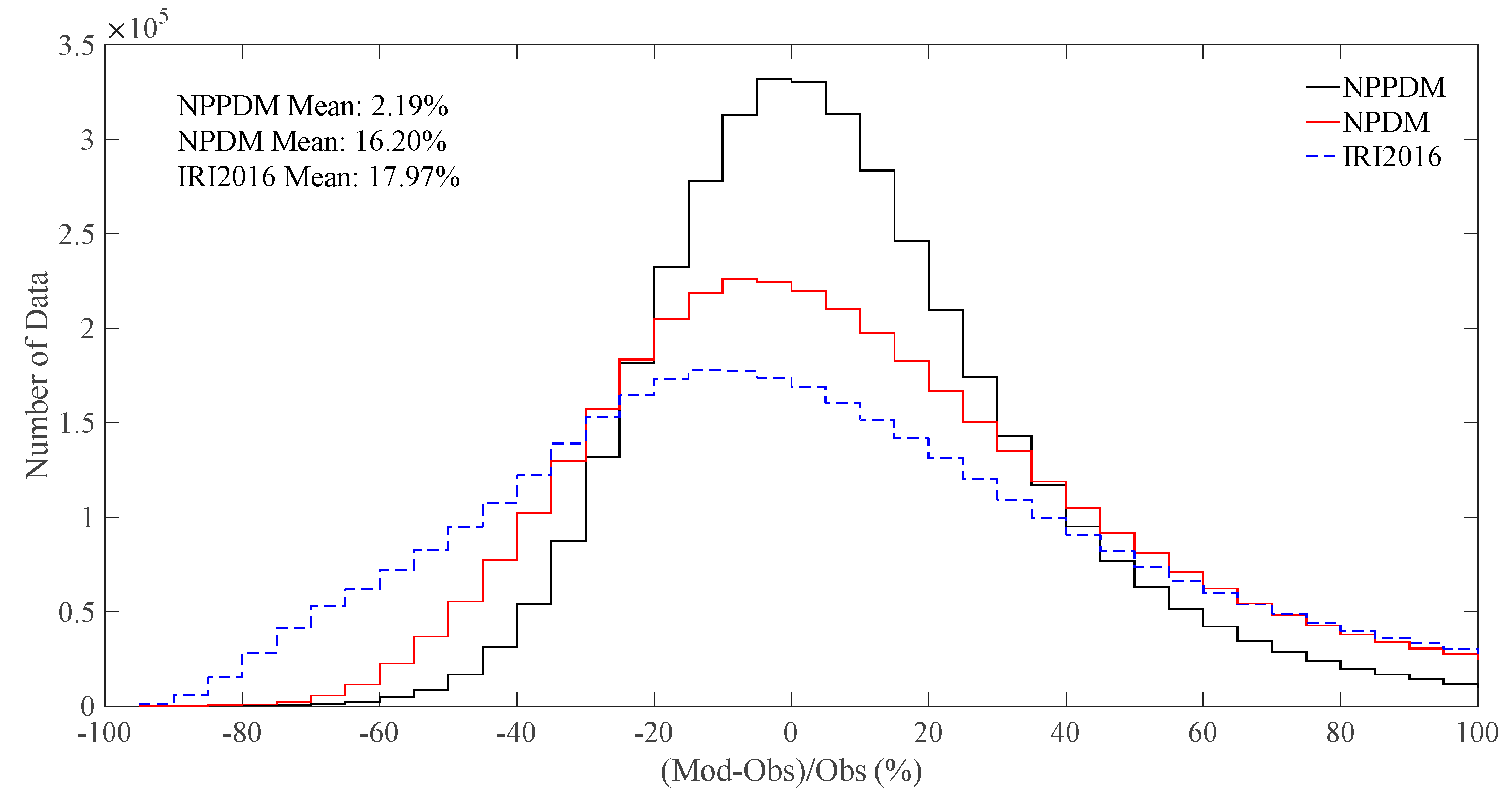
Figure 2 shows the statistical result of the relative deviations. For comparison, the residuals of IRI2016 and NPDM are also shown in Figure 2. It can be seen from Figure 2 that the NPPDM histogram peaks at −5–0% and declines steeply in both positive and negative directions. The mean relative deviations of NPPDM, IRI2016, and NPDM are 2.19%, 17.97%, and 16.20%, respectively. The large difference of IRI2016 and NPDM is mainly caused by the systematic deviation between IRO NmF2 and ionosonde NmF2 (used by IRI2016 and NPDM). The distributions of the three models show similar asymmetric patterns: the positive tail is longer than the negative tail. Generally, NPPDM can well reproduce the input database.
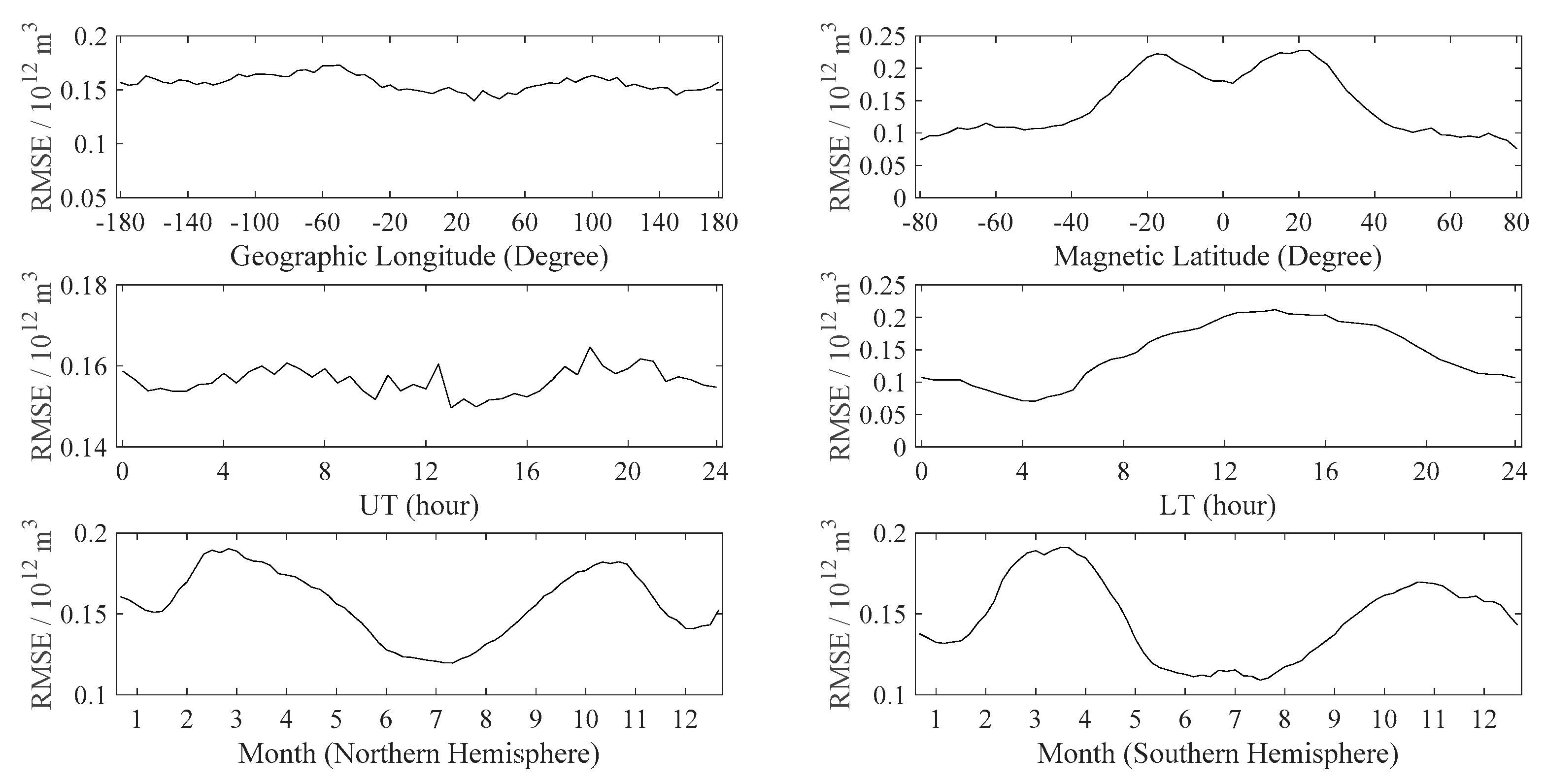
The distributions of RMSE with geographical longitude, magnetic latitude, universal time, local time (LT), and day of year are shown in Figure 3. From this figure, it can be seen that the RMSE shows no obvious differences with variations of geographical longitude and universal time. The RMSE is larger in low latitude regions than in middle and high latitude regions and shows two peaks near . The reason for this may be the EIA, which makes the variation of the F2-layer in low latitude regions a non-linear dynamic process and a result of complex physical systems [47]. It can be seen that the RMSE is larger in equinoxes than in solstices over both the northern and southern hemispheres. This can be explained by the fact that the ionospheric ionization is higher during equinoxes than during other periods. Similarly, RMSE begins to rise from sunrise as a result of the ionization increase [48].
4.2. Independent Test with Occultation Data
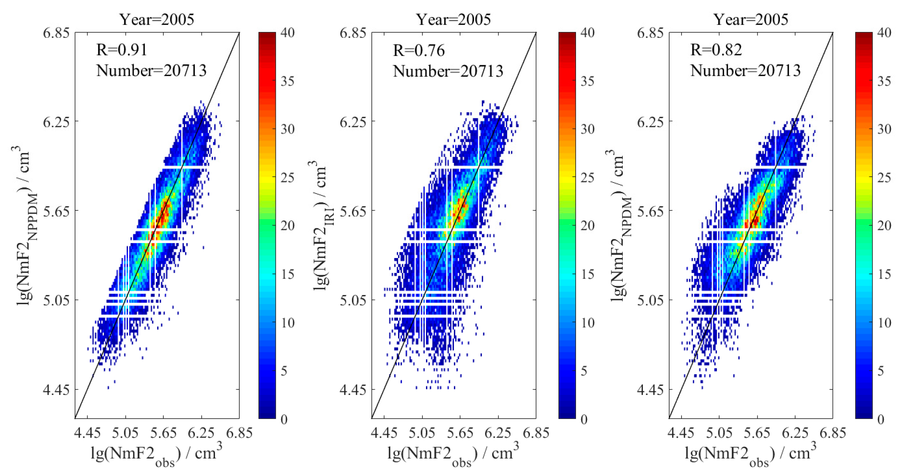
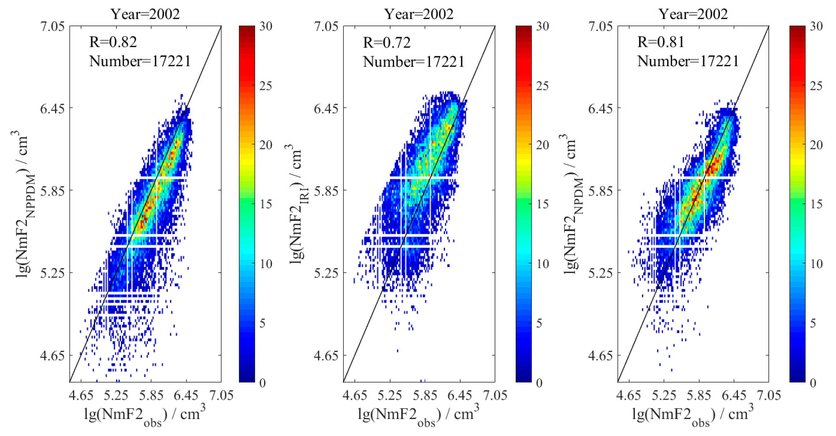
In this part, the IRO data for the years 2002 and 2005 were selected for comparisons among the model predictions of NPPDM, IRI2016, and NPDM. It should be pointed out that the NPPDM model we validate here is a reconstructed one, after removing the observational IRO data for 2002 and 2005 from the database. Therefore, the data used here for validation were independent and outside the window of the database. The solar activity was at relatively low and high levels in 2005 and 2002, respectively. Note that the data for these two years cover wide ranges of latitude, longitude, universal time, and day of year. The reproduction results for 2005 and 2002 are shown in Figure 4 and Figure 5, respectively. The diagonal line depicts perfect prediction. Several white lines can be seen in the two figures for the reason that the corresponding values are missing in the data for these two years. The correlation coefficient (R) was calculated for quantitative analysis.
In 2005, the correlation coefficient between NPPDM predictions and IRO measurements is 0.91, higher than that of IRI2016 and NPDM, for which the values are 0.76 and 0.82, respectively. It should be noted that NPPDM used only IRO NmF2 for construction, while IRI2016 used ionosonde NmF2, and NPDM included both in its data source. Therefore, it is not surprising that NPPDM and NPDM show better performances when compared with IRO NmF2. In 2002, NPDM, NPPDM, and IRI2016 show the correlation coefficients of 0.81, 0.82, and 0.72, respectively. However, it can be seen that NPPDM shows a longer tail below the diagonal line than other models and does not distributes as tightly as NPDM. Note that the IRO data in 2002 was included in the database for NPDM, but it is outside the database for NPPDM validated here. The decrease of the accuracy of NPPDM in 2002 may be due to the poor coverage of source data under high solar activity. The COSMIC mission started at 2006 and the peak of the last solar cycle with the highest F10.7 values happened during 2000—2002. Actually, CHAMP mission partly covers this period. However, due to its single satellite, not much data is available.
4.3. Independent test with Ionosonde Data
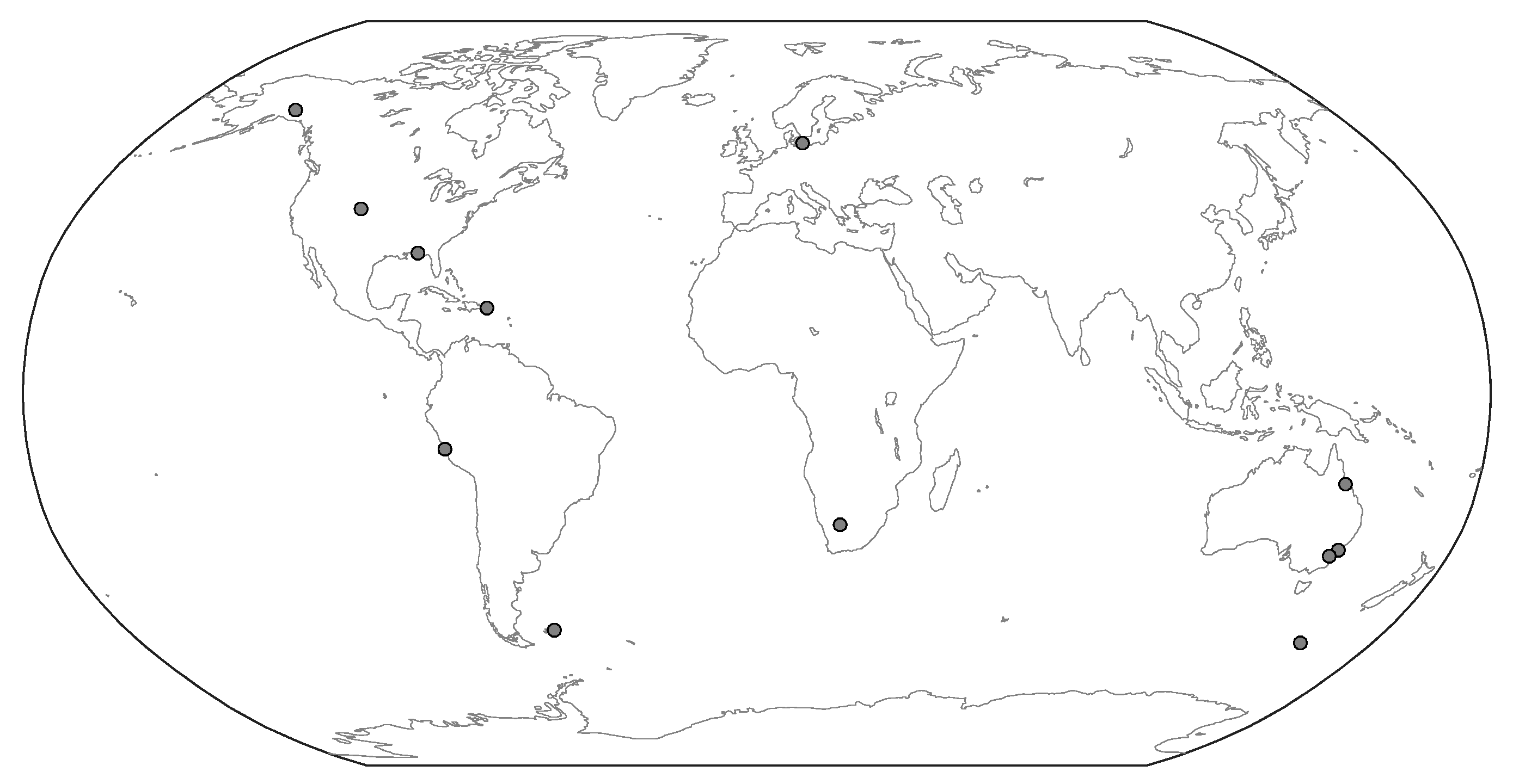
We used ionosonde measurements from twelve different stations worldwide to validate NPPDM. The ionosonde observations during low (2007 and 2008) and high (2013 and 2014) solar activity years were selected, covering the months of June, March, September, and December in the temporal range, which represented the four seasons of spring, summer, autumn, and winter, respectively. As for the spatial range, the chosen stations were distributed on both sides of the equator in low, middle, and high latitude regions, covering America, Europe, and Oceania in the eastern and western hemispheres. Table 2 shows the geographical coordinates and the validation periods of all selected stations. A global map showing geographical locations of the selected ionosonde stations is presented in Figure 6.
The ionosonde measurements were averaged at each UT hour for all days in the selected months. Afterwards, the corresponding hourly means were reproduced by NPPDM, IRI2016, and NPDM, respectively. Analog deviations between ionosonde observations and model predictions were calculated. The analog deviation not only considers the shape analog but also magnitude analog between samples [49]. The analog deviation () of two samples can be expressed by
where
Here, denotes the mean deviation. is actually the mean value of absolute distance, which is able to accurately reflect the deviation degree in the total means of two samples, and therefore called the magnitude coefficient. reflects the discrete degree of the element difference from of the two samples. Obviously, only when each equals , then , and the shapes of the two sample curves are completely similar; conversely, the larger the discrete degree of each from , the more dissimilar the two sample curves are. It is known from the above that is able to better reflect the analog degree in shapes of two samples, and is thus called the shape coefficient. Expression (19) was used for data normalization in this study before the analog deviation was calculated,
where is the original value, is the normalized value, and are the minimum and maximum values of the original data, respectively.
It can be proven that . The less the value of is, the more analogous the two samples are.
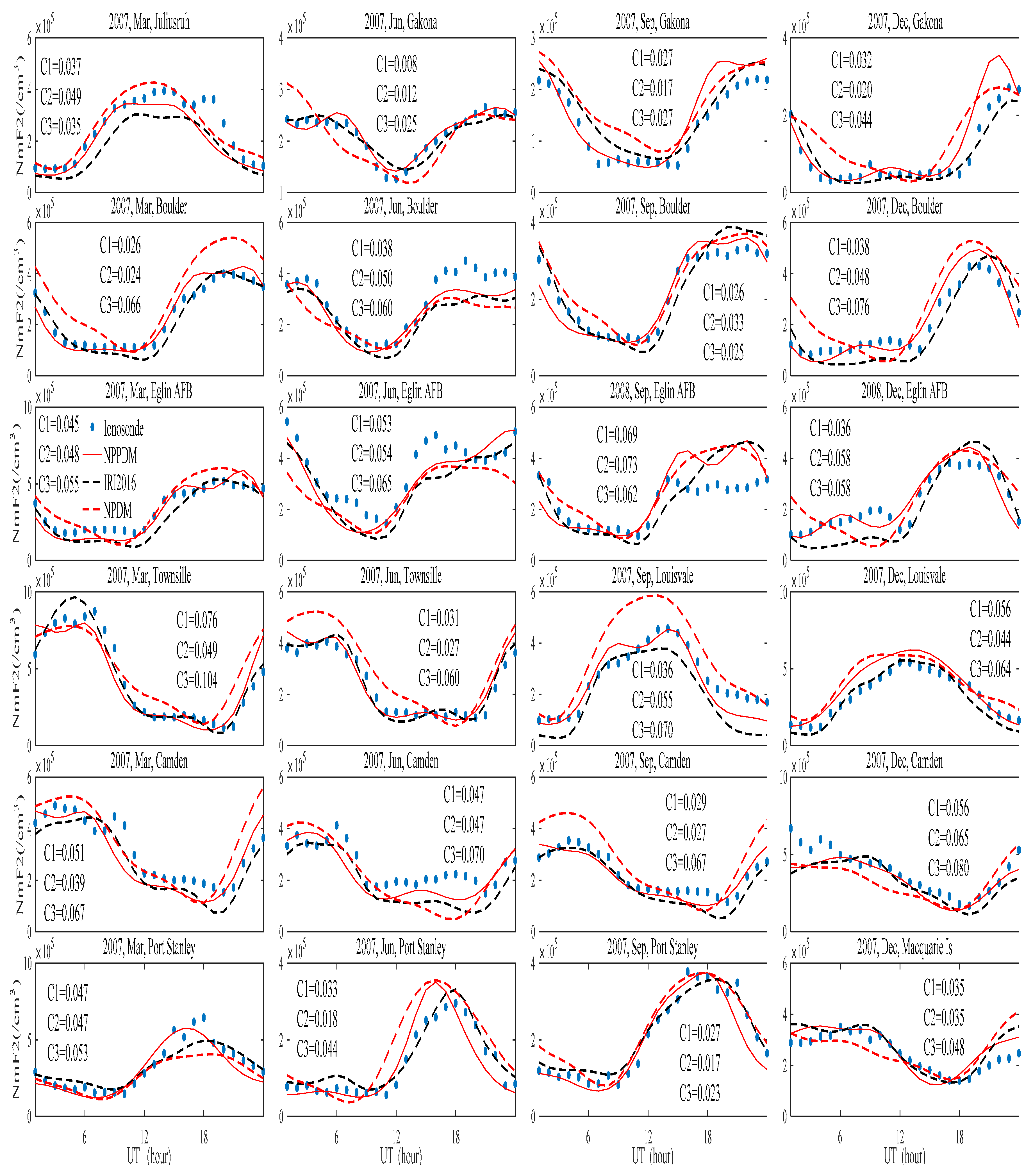
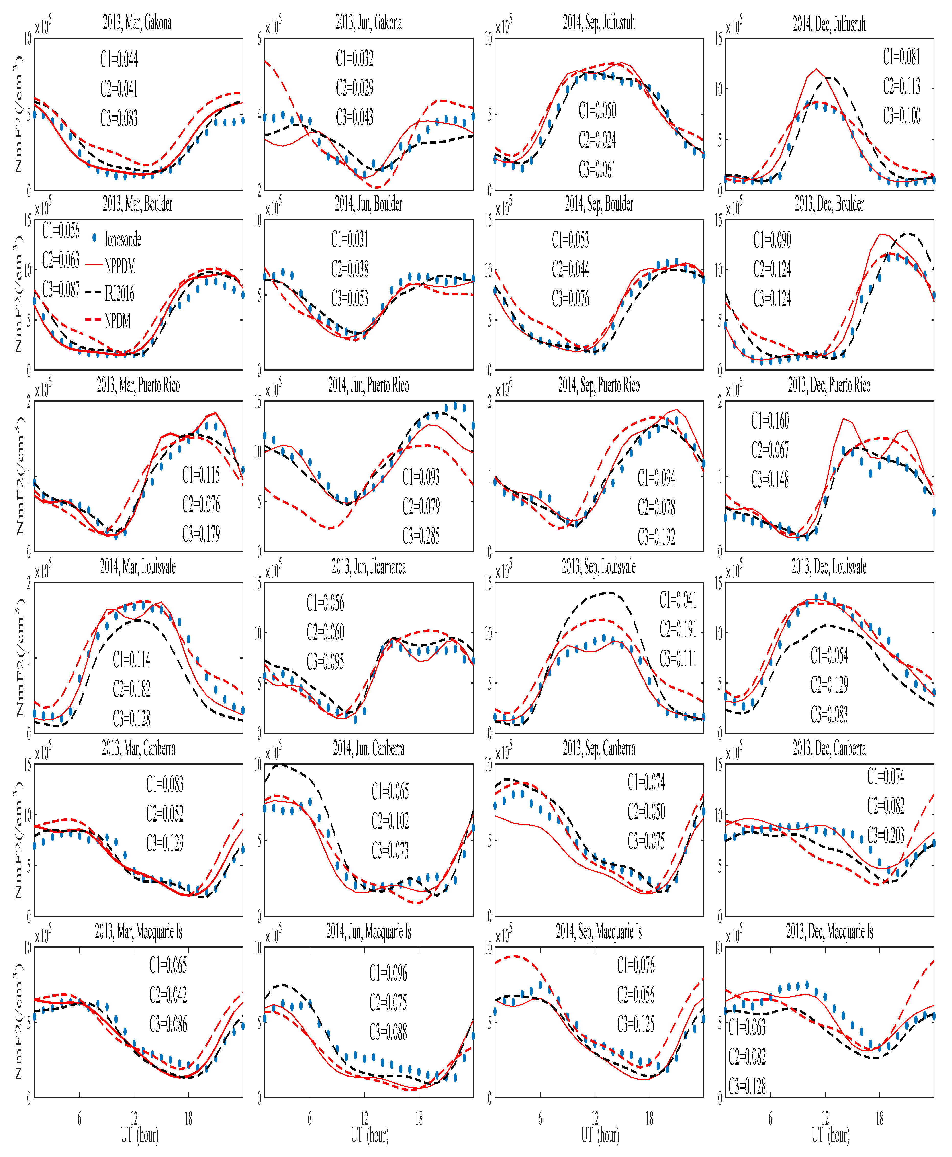
The comparisons between model predictions and ionosonde observations are shown in Figure 7 and Figure 8, corresponding to low and high solar activity, respectively. It can be seen from Figure 7 and Figure 8 that NPPDM could not only reproduce actual measurements with small differences in values, but also describe the diurnal variation trend with small discrepancies. In Figure 7 and Figure 8, NPDM shows larger analog deviations than NPPDM over majority of the selected stations, and this is especially true when the shape analog is considered. Note that the NPDM model used data until 2010, so its performance may be relative inferior when compared with data after 2010. The models with the smallest analog deviations in low (0°–30°), middle (30°–50°), and middle-high (>50°) latitude stations under low and high solar activity (as displayed in Figure 7 and Figure 8) are listed in Table 3 and Table 4, respectively. It can be seen from Table 3 and Table 4 that NPPDM, IRI2016, and NPDM show the smallest analog deviations in 24, 25, and 2 station-month validations (as displayed in each subplot of Figure 7 and Figure 8), respectively. Therefore, we can find that the performance of NPPDM is comparable to that of IRI2016. It is expected that the accuracy of NPPDM has not been improved significantly compared with IRI2016 when ionosonde data were used for comparisons, because ionosonde data were used in the IRI model development, but were not included in the database of NPPDM.
4.4. Ionospheric Features Simulation
Hoque and Jakowski [27] used the similar approach and developed an NmF2 model (Neustrelitz Peak Density Model—NPDM) with 13 model coefficients. In their model, F10.7, DOY, LT, Lat and Mlat were chosen as input elements to describe the dependencies of NmF2. They included longitude behavior by virtue of the local time term. This local time coordinate, however, did not allow them to model non-migrating tides or other non-sun-fixed features. Figure 9 and Figure 10 show the global constant local time maps of NmF2 predicted by NPDM. Note that the local time is fixed, while the universal time changes along the horizontal axis in each submap of Figure 9 and Figure 10. As shown in Figure 9 and Figure 10, the well-known longitudinal structure in the low-latitude ionosphere (wavenumber-4, WN4) cannot be displayed by NPDM. According to the previous studies, the WN4 patterns in the F2 region mainly result from the influence of the lower atmospheric non-migrating tide through either interaction with the neutral background and the ionosphere itself or modulating the E region dynamo [50,51,52]. Therefore, it is necessary to do a preliminary verification of the NPPDM’s capability to capture ionospheric features.
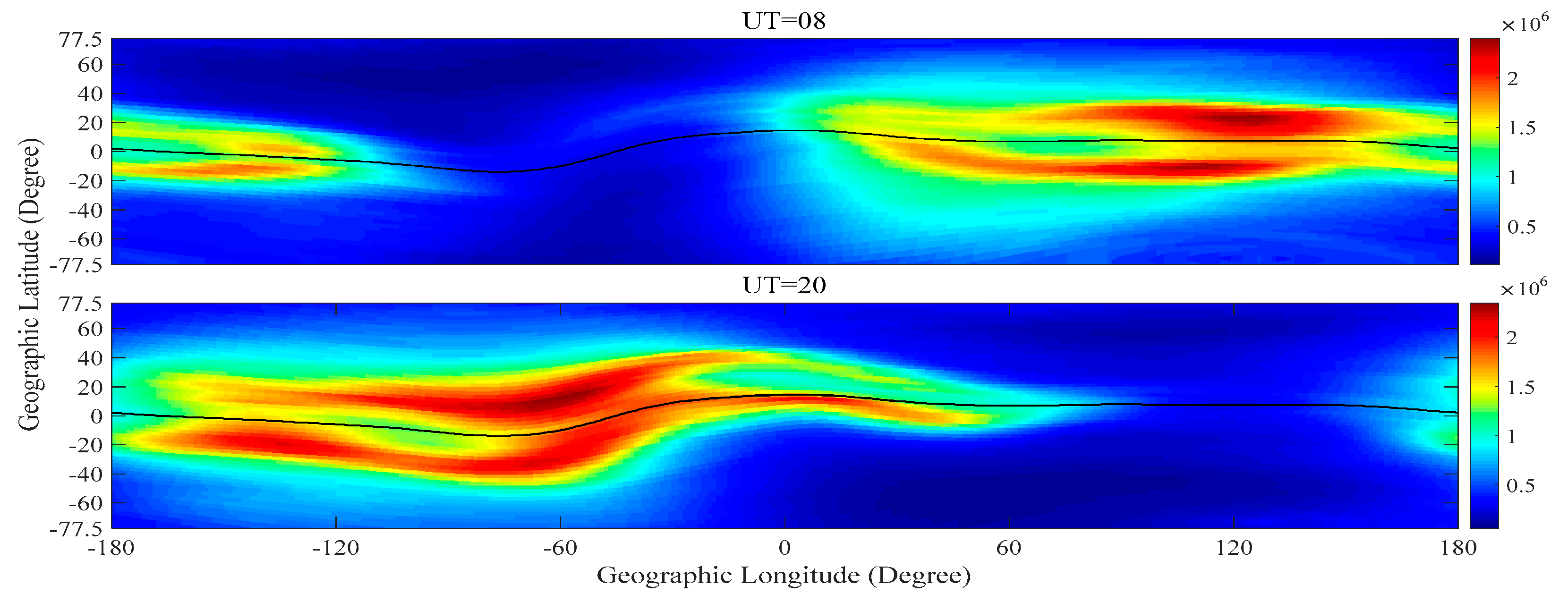
To validate the capability of NPPDM to present the expected latitudinal features, the global distributions of NmF2 at 08 UT and 20 UT under moderate solar activity (F10.7 = 120 sfu) produced by NPPDM at the September equinox are shown in Figure 11. In the day sector of Figure 11, when the ionosphere is irradiated, a pronounced double peak centers around ±20–±40° dip on either side of the magnetic dip equator (black curves), which is known as the EIA. This phenomenon is induced by the well-known fountain effect, which lifts the equatorial plasma through to a height of several hundreds of kilometers [53,54]. The plasma diffuses downward along magnetic field lines under the influence of gravity and pressure gradient forces after the plasma is lifted to greater heights. In Figure 11, the EIA asymmetry is also shown: the denser Nmf2 is in either the northern or the southern hemisphere, where neutral winds are equatorward [55].
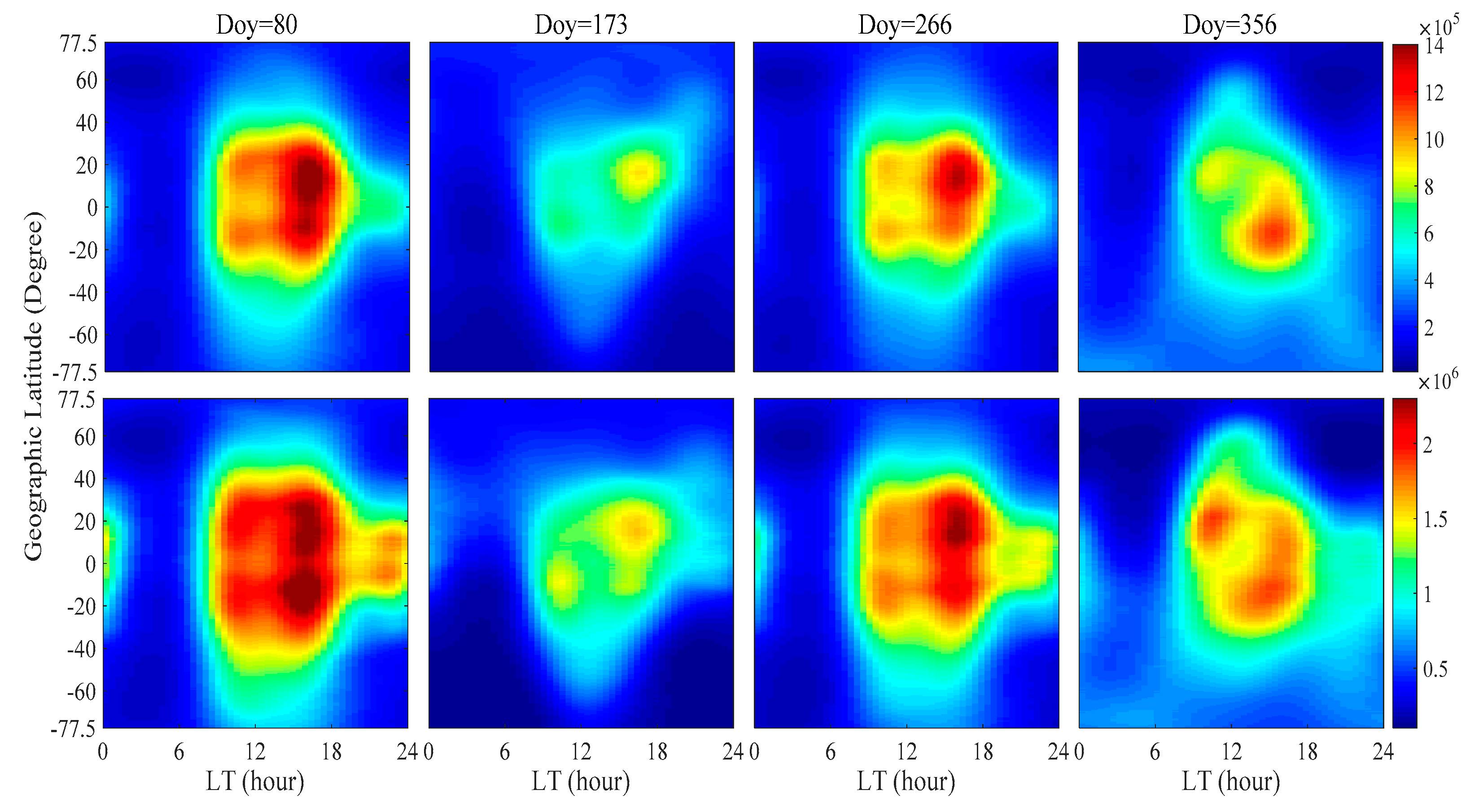
Figure 12 shows the longitudinal mean LT-Lat maps of NmF2 reproduced by NPPDM in equinoxes and solstices. Results are considered under both low (F10.7 = 80 sfu) and high (F10.7 = 150 sfu) solar activities. The EIA is also shown in each submap in Figure 12. In the daytime, a trough around the geomagnetic equator and two crests in either side of the equator can be found. After the sunset, the two crests on both sides of the geomagnetic equator gradually recede and merge into one, and finally disappear. In addition, some other features of NmF2 can be seen in Figure 12. NmF2 increases due to the solar activity enhancement. NmF2 is found to be higher in equinoxes than in solstices. This semi-annual variation is attributed to the neutral O/N2 concentration ratio variation according to the previous study [56]. The hemispheric asymmetry is also illustrated in Figure 12: NmF2 is higher in the summer hemisphere than in the winter hemisphere, and the EIA daily NmF2 peaks appear earlier in the winter hemisphere than in the summer hemisphere. The hemispheric asymmetry presented here agrees well with previous results [57,58].
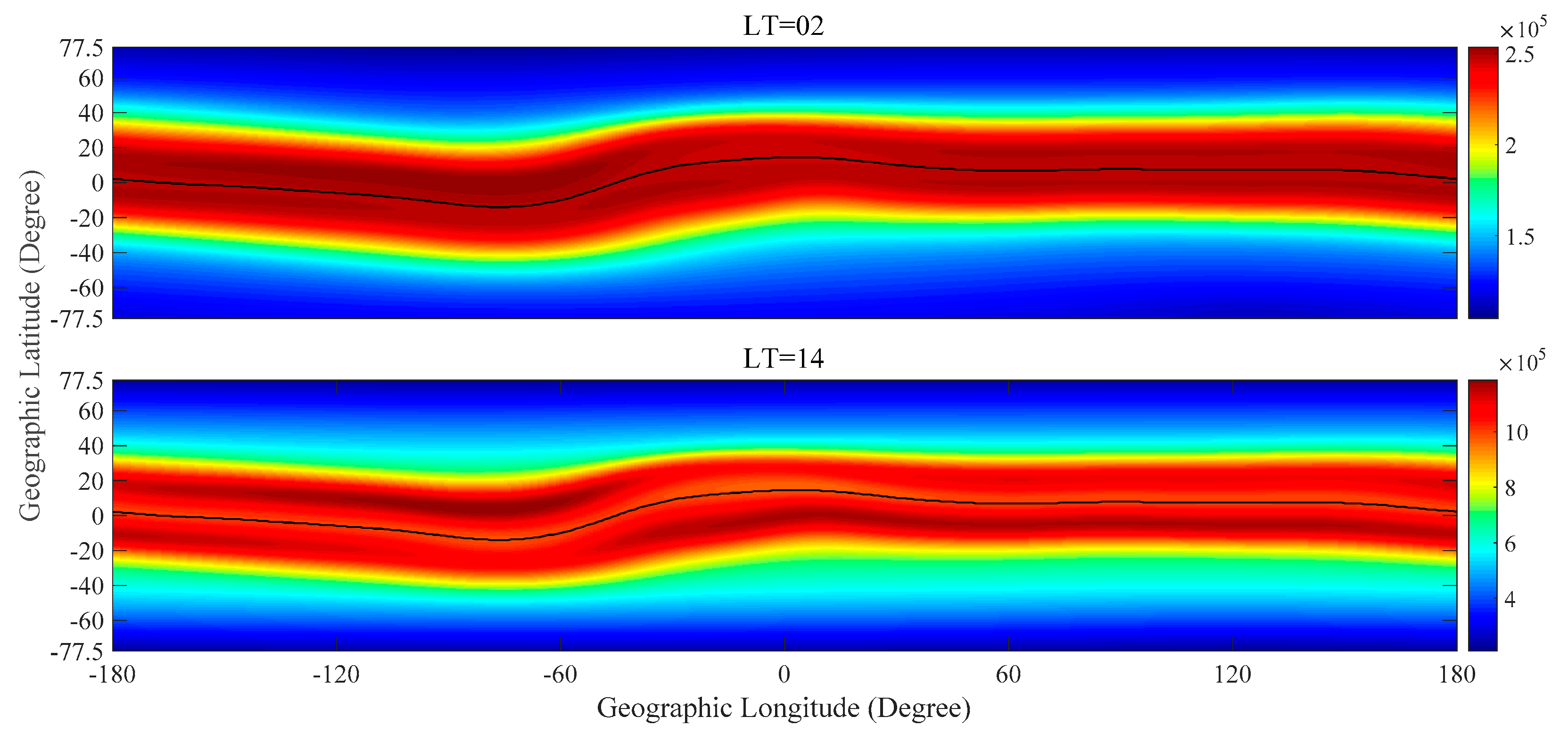
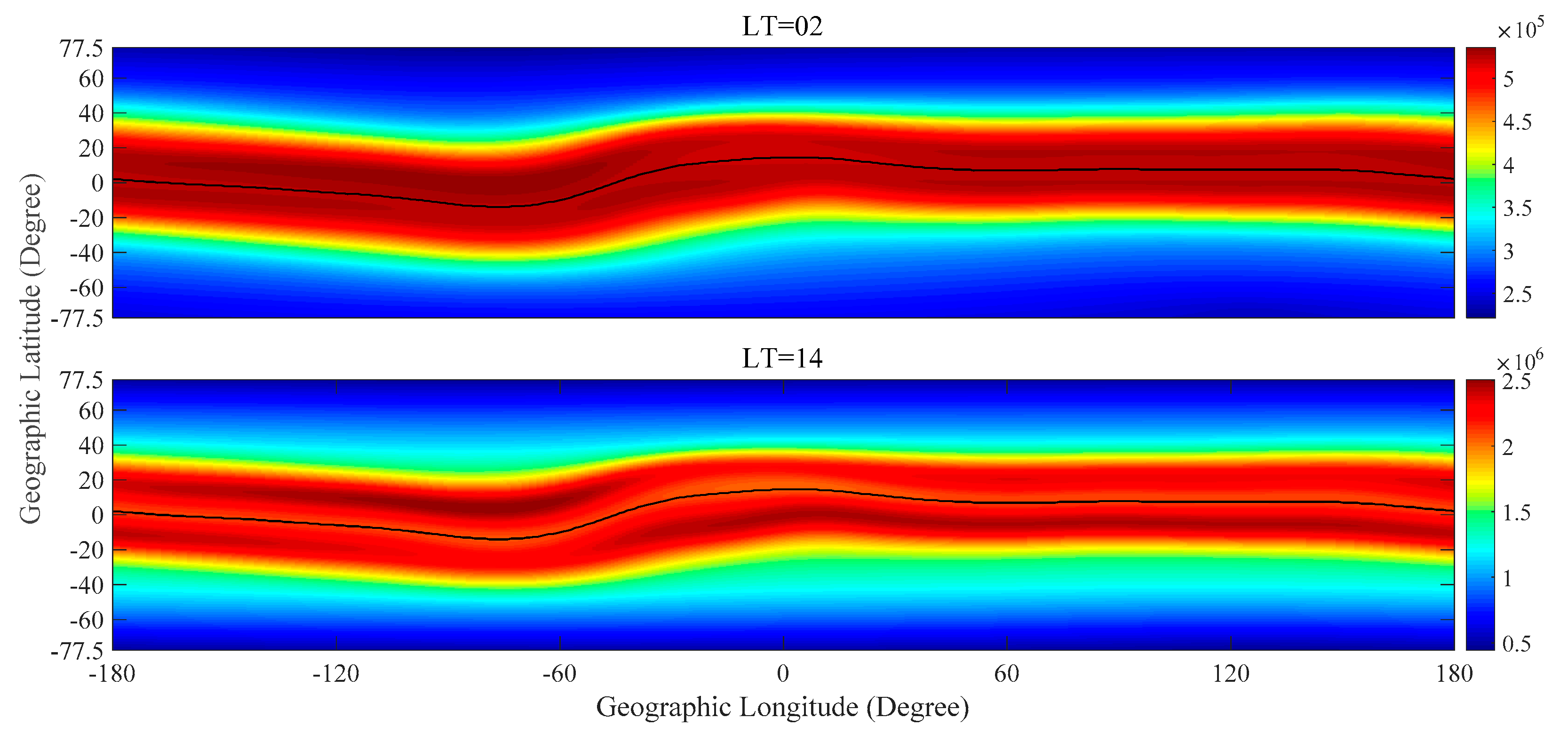
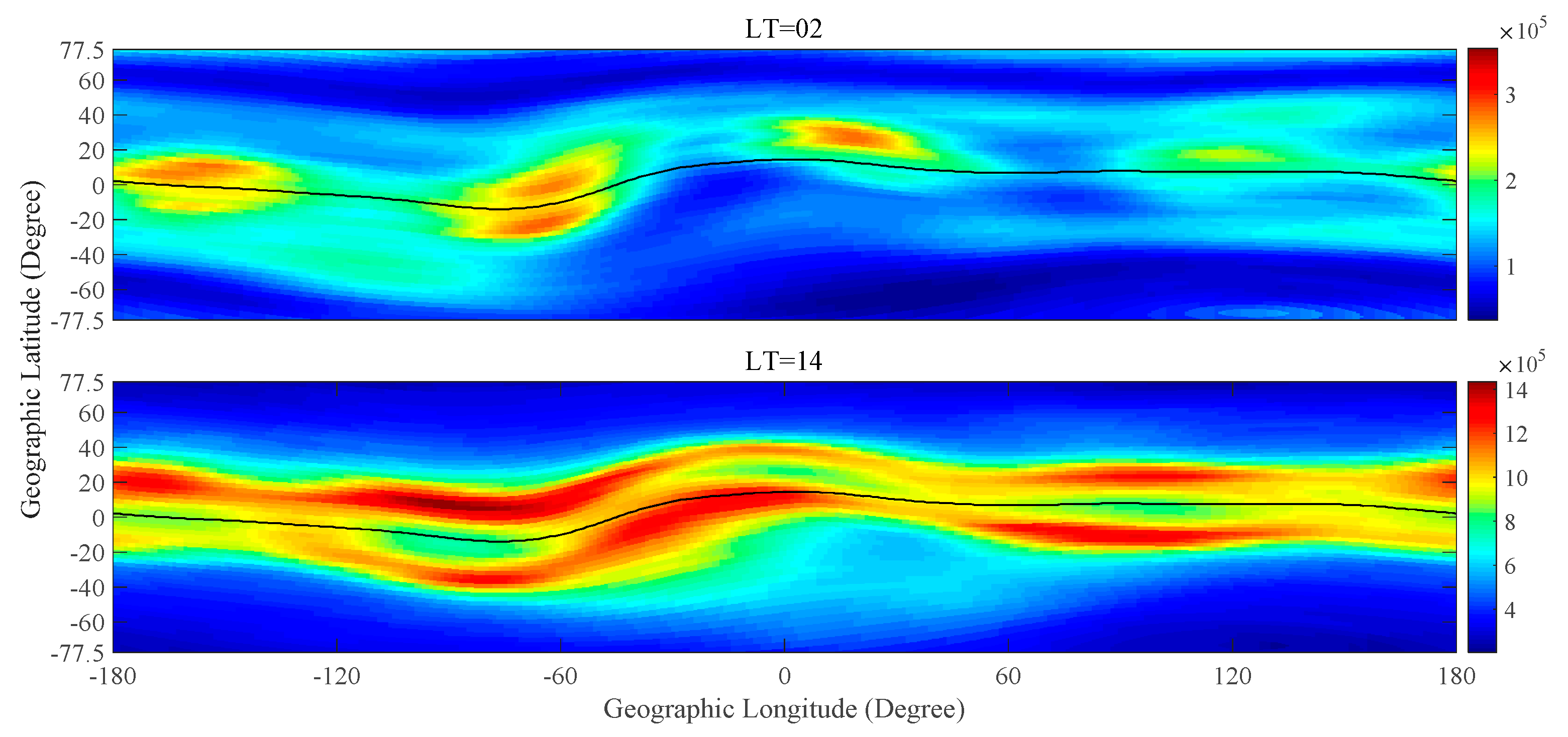
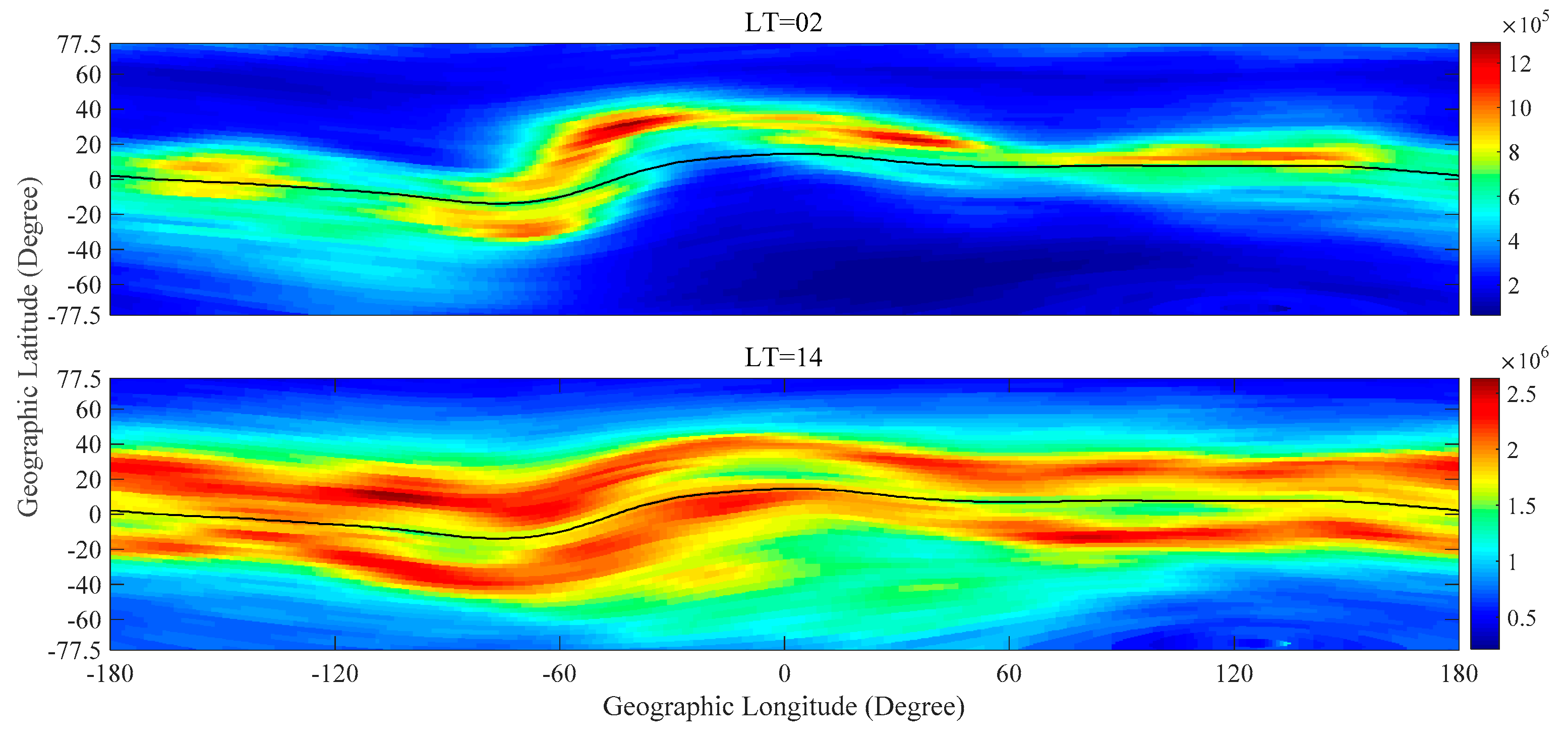
Latitude versus longitude distributions of NmF2 at 02 LT and 14 LT produced by NPPDM at the September equinox are displayed in Figure 13 and Figure 14, corresponding to low (F10.7 = 80 sfu) and high (F10.7 = 150 sfu) solar activity, respectively. We can see from the figures that WN4 patterns are shown at 14LT: the EIA crests are enhanced over West Africa, Southeast Asia, Central Pacific Ocean, and South America. The satellite observations of different ionospheric parameters, such as total electron content (TEC) and hmF2 also present WN4 longitude structures [59,60,61,62]. However, probably because the wave-like longitude structures were observed by quasi-sun-synchronous satellites, they have been researched only at fixed local time (LT) mostly before. Using NPPDM, the development and propagation of the wave-like patterns can be further investigated. Beyond this, it can be seen that a large-scale electron density depletion structure appears near latitudes at 02 LT. This ionospheric midlatitude trough is also described by NPPDM, which forms at the interface between the midlatitude ionosphere and the high-latitude auroral region as a result of the complex interplay between different geophysical processes [63]. We have noticed the enhancement of NmF2 at 02 LT at high latitudes, which is caused by the disappearance of photoionization at middle latitudes and auroral particle precipitation at high latitudes [64].
5. Discussion
Recently, Sai and Tulasi [24] developed ANNIM to predict global NmF2 based on COSMIC data. Afterwards, Tulasi et al. [25] presented an improved version of ANNIM by assimilating more IRO measurements as well as ionosonde data using a modified spatial gridding approach based on the magnetic dip latitudes. They used an Artificial Neural Networks technique, which enabled the estimation of the coefficients without knowing the base function of independent variables in advance. More variables were selected as inputs in their model than NPPDM, including DOY, UT, latitude, longitude, F10.7, Kp, declination, inclination, dip latitude, zonal wind, and meridional wind. The Kp input enabled ANNIM to operate under disturbed geomagnetic conditions and to be more applicable than NPPDM, which is only effective under quiet and moderate geomagnetic conditions [25]. As declared by Sai and Tulasi [24], ANNIM showed the regression coefficient of 0.89 when compared with the GRACE data. It can be seen from Figure 4 and Figure 5 (in this paper) that NPPDM is well linearly correlated with the independent IRO data. For comparison, the regression coefficients in Figure 4 and Figure 5 for 2005 and 2002 were calculated and show values of 0.96 and 0.77, respectively. The relative low value of the regression coefficient in 2002 can be due to the poor coverage of source data under high solar activity, as we mentioned above in Section 4.2. Therefore, we think that the performance of NPPDM is generally comparable with that of ANNIM. However, the validation data set (15% of total data), which was prepared for the validation process to avoid the overfitting of ANNIM parameters and to ensure the errors were within the permissible range, was outside the database and was not used to derive the non-linear relationship or the coefficients of the empirical model. Thus, it is possible that the ANNIM has a limitation over high latitude areas, where the data distribution is relatively sparse. As mentioned by Sai and Tulasi [24], ANNIM underestimated the NmF2 at high latitudes and the mean relative deviation increased to ~20–25% when compared with IRO data. We have calculated the mean relative deviation of NPPDM based on the same measurements from the four high latitude ionosonde stations (Gakona, Juliusruh, Macquarie Is, and Port Stanley) in Figure 7 and Figure 8. The result shows a mean relative deviation of 14%. Note that the deviation for NPPDM may be even smaller when compared with IRO data due to the systematic deviation between ionosonde NmF2 and occultation NmF2 (used as data source by NPPDM). In addition, the performance of ANNIM in higher latitudes (>60°) has not been reviewed in their studies, while it can be seen from this work that NPPDM shows a reasonable performance there and well presents the midlatitude trough near ±60° latitudes (Figure 13 and Figure 14).
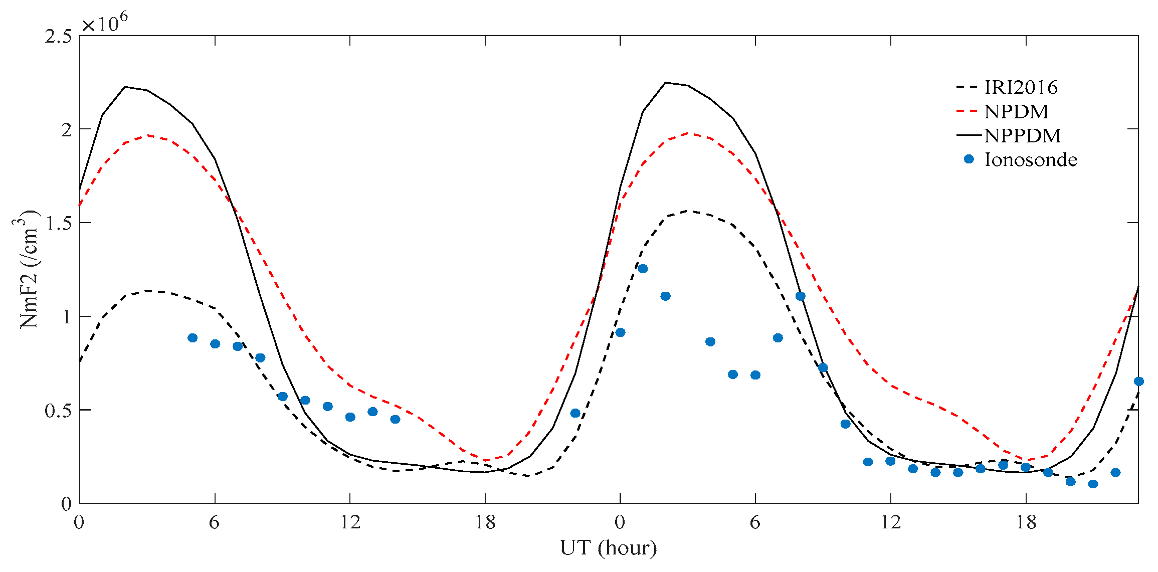
It is known that geomagnetic storms may profoundly affect the variation of NmF2. However, NPPDM was designed for quiet and moderate geomagnetic conditions and the IRO measurements under disturbed geomagnetic conditions (Ap > 32) were removed from the database when the model was developed. Therefore, it should be noted that our model may show large errors during storm events. Jin et al. [65] reported a fairly large increase of NmF2 during the super geomagnetic storm (20 November 2003) at Anyang station (37.4°N, 127.0°E). Figure 15 shows the NmF2 hourly variations of ionosonde observations and model predictions at Anyang station for a 2-day period (20–21 November 2003). The variation of Kp index during this period can be seen in Jin’s paper (Figure 4). Some ionosonde measurements are missing due to the absorption during the storm. The predictions using the STORM version of the IRI2016 are presented in Figure 15 (black dotted lines). The STORM model [14] was included in IRI and was designed to be dependent on the intensity of the storm (ap index over the 33 previous hours), latitude, and season. In Figure 15, the abnormal variations of ionosonde NmF2 during 10 to 14 UT (20, November) and 02 to 07 UT (21, November) may be associated with the variations of geomagnetic activity. The limitation of NPPDM during storm can be seen in Figure 15. We can see that IRI2016 (STORM on) shows the best performance between the three models, while NPPDM and NPDM mainly overestimate the NmF2 during this storm event. Joshua et al. [66] reported that NmF2 was more perturbed than TEC, which further stressed the importance of NmF2 in ionospheric modeling, particularly during disturbed geophysical conditions. Therefore, further research on solving this limitation of NPPDM is needed.
The F2-layer peak density height hmF2 is another important parameter in empirical ionospheric modeling. Hoque and Jakowski [67] followed the same basic approach and developed a nonlinear hmF2 model in another paper. Therefore, the approach we used in this paper may have the potential application in hmF2 modeling. This possibility requires more investigations. Since the hmF2 modeling is beyond the scope of this paper, further research will be performed in the future.
6. Conclusions
In this study, an empirical model NPPDM was developed based on CHAMP, GRACE, and COSMIC radio occultation data. The model was designed as a simple pattern consisting of nonlinear polynomial equations to describe the dependences of NmF2 on universal time, day of year, solar activity, and longitude. We divided the globe into 63 slices according to the geomagnetic latitude. The coefficients were derived by a multivariable fitting in each latitude slice. To validate the model, the predictions of NPPDM were compared with IRO data and ionosonde data, as well as the predictions of the IRI2016 and NPDM models. In addition, we simulated some ionospheric climatological features using the new model. The simulation shows good agreement with the previous observational conclusions. The main results can be summarized as follows:
- Using NPPDM to reproduce the input data, the mean relative deviation between the input data and the new model is 2.19%. NPPDM shows larger RMSE in the EIA region than in other regions.
- The predictions of NPPDM were compared with independent IRO measurements, IRI2016 predictions, and NPDM predictions. The correlation coefficients between model predictions and actual measurements show that the NPPDM performs better than IRI2016 and NPDM under low solar activity, while it undergoes performance degradation under high solar activity as a result of the poor database coverage.
- Ionosonde data from twelve stations were selected to validate the accuracy of NPPDM. The analog deviations between ionosonde observations and model predictions indicate that the precision of NPPDM is better than that of NPDM and comparable to that of IRI2016.
- The variations and distributions of NmF2 simulated by NPPDM agree well with previous research. NPPDM can capture some ionospheric features including the EIA, the longitudinal wavenumber-4 structure, and the midlatitude trough.
Supplement of the database from upcoming satellite missions, especially under high solar activity, is required to further improve the model.
Author Contributions
Conceptualization of the Manuscript Idea: H.F. and Z.L.; Methodology and Software: Z.L. and M.M.H.; Writing Original Draft: Z.L. and L.W.; Writing—Review: M.M.H., S.Y. and Z.G.
Acknowledgments
The authors are grateful to sponsors and operators of the CHAMP and GRACE missions; Deutsches GeoForschungs Zentrum (GFZ) Potsdam, German Aerospace Center (DLR), and the US National Aeronautics and Space Administration (NASA). The authors would like to give thanks to sponsors and operators of the FORMOSAT-3/COSMIC mission; Taiwan’s National Science Council and National Space Organization (NSPO), the US National Science Foundation (NSF), National Aeronautics and Space Administration (NASA), National Oceanic and Atmospheric Administration (NOAA) and the University Corporation for Atmospheric Research (UCAR). The authors are also grateful to NGDC for disseminating historical ionosonde data via SPIDR.
Conflicts of Interest
The authors declare no conflict of interest.
References
- Davies, K. Ionospheric Radio; Peter Peregrinus on behalf of the Institution of Electrical Engineers: London, UK, 1990. [Google Scholar]
- Farelo, A.F.; Herraiz, M.; Mikhailov, A.V. Global morphology of night-time NmF2 enhancements. Ann. Geophys. 2002, 20, 1795–1806. [Google Scholar] [CrossRef]
- Halcrow, B.W.; Nisbet, J.S. A model of F2 peak electron densities in the main trough region of the ionosphere. Radio Sci. 1977, 12, 815–820. [Google Scholar] [CrossRef]
- Rush, C.M.; Pokempner, M.; Anderson, D.N.; Stewart, F.G.; Perry, J. Improving ionospheric maps using theoretically derived values of foF2. Radio Sci. 1983, 18, 95–107. [Google Scholar] [CrossRef]
- Fox, M.W.; McNamara, L.F. Improved world-wide maps of monthly median of foF2. J. Atmos. Terr. Phys. 1988, 50, 1077–1086. [Google Scholar] [CrossRef]
- Bilitza, D.; Altadill, D.; Truhlik, V.; Shubin, V.; Galkin, I.; Reinisch, B.; Huang, X. International Reference Ionosphere 2016: From ionospheric climate to real-time weather predictions. Space Weather 2017, 15, 418–429. [Google Scholar] [CrossRef]
- Bilitza, D.; Reinisch, B.W. International reference ionosphere 2007: Improvements and new parameters. Adv. Space Res. 2008, 42, 599–609. [Google Scholar] [CrossRef]
- Fuller-Rowell, T.J.; Araujo-Pradere, E.; Codrescu, M.V. An empirical ionospheric storm-time correction model. Adv. Space Res. 2000, 25, 139–146. [Google Scholar] [CrossRef]
- Radicella, S.M.; Leitinger, R. The evolution of the DGR approach to model electron density profiles. Adv. Space Res. 2001, 27, 35–40. [Google Scholar] [CrossRef]
- Coïsson, P.; Radicella, S.M.; Leitinger, R.; Nava, B. Topside electron density in IRI and NeQuick: Features and limitations. Adv. Space Res. 2006, 37, 937–942. [Google Scholar] [CrossRef]
- Nava, B.; Coïsson, P.; Radicella, S.M. A new version of the NeQuick ionosphere electron density model. J. Atmos. Sol. Terr. Phys. 2008, 70, 1856–1862. [Google Scholar] [CrossRef]
- CCIR (Consultative Committee on International Radio). Atlas of Ionospheric Characteristics Report 340; International Telecommunication Union: Geneva, Switzerland, 1967. [Google Scholar]
- Rush, C.M. URSI foF2 model maps (1988). Planet. Space Sci. 1992, 40, 546–547. [Google Scholar] [CrossRef]
- Araujo-Pradere, E.A.; Fuller-Rowell, T.J.; Codrescu, M.V. STORM: An empirical storm-time ionospheric correction model 1. Model description. Radio Sci. 2002, 37, 1070. [Google Scholar] [CrossRef]
- Oyeyemi, E.O.; McKinnell, L.A. A new global F2 peak electron density model for the International Reference Ionosphere (IRI). Adv. Space Res. 2008, 42, 645–658. [Google Scholar] [CrossRef]
- Liu, C.; Zhang, M.; Wan, W.; Liu, L.; Ning, B. Modeling M(3000)F2 based on empirical orthogonal function analysis method. Radio Sci. 2008, 43, RS1003. [Google Scholar] [CrossRef]
- Zhang, M.; Liu, C.; Wan, W.; Liu, L.; Ning, B. A global model of the ionospheric F2 peak height based on EOF analysis. Ann. Geophys. 2009, 27, 3203–3212. [Google Scholar] [CrossRef] [Green Version]
- Zhang, D.H.; Xiao, Z.; Hao, Y.Q.; Ridley, A.J.; Moldwin, M. Modeling ionospheric foF2 by using empirical orthogonal function analysis. Ann. Geophys. 2011, 29, 1501–1515. [Google Scholar] [Green Version]
- Kumluca, A.; Tulunay, E.; Topalli, I.; Tulunay, Y. Temporal and spatial forecasting of ionospheric critical frequency using neural networks. Radio Sci. 1999, 34, 1497–1506. [Google Scholar] [CrossRef]
- Oyeyemi, E.O.; Poole, A.W.V.; McKinnell, L.A. On the global model for foF2 using neural networks. Radio Sci. 2005, 40, RS6011. [Google Scholar] [CrossRef]
- Oyeyemi, E.O.; McKinnell, L.A.; Poole, A.W.V. Near-real time foF2 predictions using neural networks. J. Atmos. Sol. Terr. Phys. 2006, 68, 1807–1818. [Google Scholar] [CrossRef]
- McKinnell, L.A.; Oyeyemi, E.O. Progress towards a new global foF2 model for the International Reference Ionosphere (IRI). Adv. Space Res. 2009, 43, 1770–1775. [Google Scholar] [CrossRef]
- McKinnell, L.A.; Oyeyemi, E.O. Equatorial predictions from a new neural network based global foF2 model. Adv. Space Res. 2010, 46, 1016–1023. [Google Scholar] [CrossRef]
- Sai Gowtam, V.; Tulasi Ram, S. An artificial neural network-based ionospheric model to predict NmF2 and hmF2 using long-term data set of FORMOSAT-3/COSMIC radio occultation observations: Preliminary results. J. Geophys. Res. Space Phys. 2017, 122, 743–755. [Google Scholar] [CrossRef]
- Tulasi Ram, S.; Sai Gowtam, V.; Mitra, A.; Reinisch, B. The improved two-dimensional artificial neural network-based ionospheric model (ANNIM). J. Geophys. Res. Space Phys. 2018, 123, 5807–5820. [Google Scholar] [CrossRef]
- Themens, D.R.; Jayachandran, P.T.; Galkin, I.; Hall, C. The Empirical Canadian High Arctic Ionospheric Model (E-CHAIM): NmF2 and hmF2. J. Geophys. Res. Space Phys. 2017, 122, 9015–9031. [Google Scholar] [CrossRef]
- Hoque, M.M.; Jakowski, N. A new global empirical NmF2 model for operational use in radio systems. Radio Sci. 2011, 46, RS6015. [Google Scholar] [CrossRef]
- Hajj, G.A.; Romans, L.J. Ionospheric electron density profiles obtained with the global positioning system: Results from the GPS.MET experiment. Radio Sci. 1998, 33, 175–190. [Google Scholar] [CrossRef]
- Garcia-Fernandez, M.; Hernandez-Pajares, M.; Juan, M.; Sanz, J. Improvement of ionospheric electron density estimation with GPSMET occultations using Abel inversion and VTEC information. J. Geophys. Res. 2003, 108, 1338. [Google Scholar] [CrossRef]
- Yue, X.; Schreiner, W.S.; Lei, J.; Sokolovskiy, S.V.; Rocken, C.; Hunt, D.C.; Kuo, Y. Error analysis of Abel retrieved electron density profiles from radio occultation measurements. Ann. Geophys. 2010, 28, 217–222. [Google Scholar] [CrossRef] [Green Version]
- Yue, X.; Schreiner, W.S.; Rocken, C.; Kuo, Y. Evaluation of the orbit altitude electron density estimation and its effect on the Abel inversion from radio occultation measurements. Radio Sci. 2011, 46, RS1013. [Google Scholar] [CrossRef]
- Lei, J.; Syndergaard, S.; Burns, A.G.; Solomon, S.C.; Wang, W.; Zeng, Z.; Roble, R.G.; Wu, Q.; Kuo, Y.; Holt, J.M.; et al. Comparison of COSMIC ionospheric measurements with ground-based observations and model predictions: Preliminary results. J. Geophys. Res. 2007, 112, A07308. [Google Scholar] [CrossRef]
- Angling, M.J. First assimilations of COSMIC radio occultation data into the Electron Density Assimilative Model (EDAM). Ann. Geophys. 2008, 26, 353–359. [Google Scholar] [CrossRef] [Green Version]
- Krankowski, A.; Zakharenkova, I.; Gregorczyk, A.K.; Shagimuratov, I.I.; Wielgosz, P. Ionospheric electron density observed by FORMOSAT-3/COSMIC over the European region and validated by ionosonde data. J. Geod. 2011, 85, 949–964. [Google Scholar] [CrossRef] [Green Version]
- Jakowski, N.; Leitinger, R.; Angling, M. Radio occultation techniques for probing the ionosphere. Ann. Geophys. 2004, 47, 1049–1066. [Google Scholar]
- Yue, X.; Schreiner, W.S.; Kuo, Y.; Lei, J. Ionosphere equatorial ionization anomaly observed by GPS radio occultations during 2006–2014. J. Atmos. Terr. Phys. 2015, 129, 30–40. [Google Scholar] [CrossRef]
- Kutiev, I.S.; Marinov, P.G.; Watanabe, S. Model of topside ionosphere scale height based on topside sounder data. Adv. Space Res. 2006, 37, 943–950. [Google Scholar] [CrossRef]
- Jakowski, N.; Hoque, M.M.; Mayer, C. A new global TEC model for estimating transionospheric radio wave propagation errors. J. Geod. 2011, 85, 965–974. [Google Scholar] [CrossRef]
- Kakinami, Y.; Watanabe, S.; Oyama, K.I. An empirical model of electron density in low latitude at 600 km obtained by Hinotori satellite. Adv. Space Res. 2008, 41, 1495–1499. [Google Scholar] [CrossRef]
- Kakinami, Y.; Chen, C.; Liu, J.; Oyama, K.I.; Yang, W.; Abe, S. Empirical models of total electron content based on functional fitting over Taiwan during geomagnetic quiet condition. Ann. Geophys. 2009, 27, 3321–3333. [Google Scholar] [CrossRef]
- Liu, H.; Hirano, T.; Watanabe, S. Empirical model of the thermospheric mass density based on CHAMP satellite observations. J. Geophys. Res. Space Phys. 2013, 118, 843–848. [Google Scholar] [CrossRef]
- Chen, Y.; Liu, L. Further study on the solar activity variation of daytime NmF2. J. Geophys. Res. 2010, 115, A12337. [Google Scholar] [CrossRef]
- Liu, H.; Stolle, C.; Förster, M.; Watanabe, S. Solar activity dependence of the electron density in the equatorial anomaly regions observed by CHAMP. J. Geophys. Res. 2007, 112, A11311. [Google Scholar] [CrossRef]
- Liu, L.; Wan, W.; Chen, Y.; Le, H. Solar activity effects of the ionosphere: A brief review. Chin. Sci. Bull. 2011, 56, 1202–1211. [Google Scholar] [CrossRef] [Green Version]
- Su, Y.; Bailey, G.J.; Fukao, S. Altitude dependencies in the solar activity variations of the ionospheric electron density. J. Geophys. Res. 1999, 104, 879–891. [Google Scholar] [CrossRef]
- Zou, L.; Rishbeth, H.; Müller-Wodarg, I.C.F.; Aylward, A.D.; Millward, G.H.; Fuller-Rowell, T.J.; Idenden, D.W.; Moffett, R.J. Annual and semiannual variations in the ionospheric F2-layer. I. Modelling. Ann. Geophys. 2000, 18, 927–944. [Google Scholar] [CrossRef]
- Watthanasangmechai, K.; Yamamoto, M.; Saito, A.; Maruyama, T.; Yokoyama, T.; Nishioka, M.; Ishii, M. Temporal change of EIA asymmetry revealed by a beacon receiver network in Southeast Asia. Earth Planet. Space 2015, 67, 75. [Google Scholar] [CrossRef]
- Adeniyi, J.O.; Joshua, B.W. Latitudinal effect on the diurnal variation of the F2 layer at low solar activity. J. Atmos. Terr. Phys. 2014, 120, 102–110. [Google Scholar] [CrossRef]
- Jin, L.; Shi, X. A Numerical Prediction Product FNN Prediction Model Based on Condition Number and Analog Deviation. In Proceedings of the Eighth ACIS International Conference on Software Engineering, Artificial Intelligence, Networking, and Parallel/Distributed Computing (SNPD 2007), Qingdao, China, 30 July–1 August 2007. [Google Scholar] [CrossRef]
- England, S.L.; Immel, T.J.; Huba, J.D.; Hagan, M.E.; Maute, A.; DeMajistre, R. Modeling of multiple effects of atmospheric tides on the ionosphere: An examination of possible coupling mechanisms responsible for the longitudinal structure of the equatorial ionosphere. J. Geophys. Res. 2010, 115, A05308. [Google Scholar] [CrossRef]
- Immel, T.J.; Sagawa, E.; England, S.L.; Henderson, S.B.; Hagan, M.E.; Mende, S.B.; Frey, H.U.; Swenson, C.M.; Paxton, L.J. Control of equatorial ionospheric morphology by atmospheric tides. Geophys. Res. Lett. 2006, 33, L15108. [Google Scholar] [CrossRef]
- Wan, W.; Liu, L.; Pi, X.; Zhang, M.; Ning, B.; Xiong, J.; Ding, F. Wavenumber 4 patterns of the total electron content over the low latitude ionosphere. Geophys. Res. Lett. 2008, 35, L12104. [Google Scholar] [CrossRef]
- Balan, N.; Bailey, G.J.; Abdu, M.A.; Oyama, K.I.; Richards, P.G.; MacDougall, J.; Batista, I.S. Equatorial plasma fountain and its effects over three locations: Evidence for an additional layer, the F3 layer. J. Geophys. Res. 1997, 102, 2047–2056. [Google Scholar] [CrossRef]
- Hanson, W.B.; Moffett, R.J. Ionization transport effects in the equatorial F region. J. Geophys. Res. 1966, 71, 5559–5572. [Google Scholar] [CrossRef]
- Balan, N.; Rajesh, P.K.; Sripathi, S.; Tulasiram, S.; Liu, J.; Bailey, G.J. Modeling and observations of the north–south ionospheric asymmetry at low latitudes at long deep solar minimum. Adv. Space Res. 2013, 52, 375–382. [Google Scholar] [CrossRef]
- Rishbeth, H.; Müller-Wodarg, I.C.F.; Zou, L.; Fuller-Rowell, T.J.; Millward, G.H.; Moffett, R.J.; Idenden, D.W.; Aylward, A.D. Annual and semiannual variations in the ionospheric F2-layer: II. Physical discussion. Ann. Geophys. 2000, 18, 945–956. [Google Scholar] [CrossRef]
- Ram, S.T.; Su, S.; Liu, C. FORMOSAT-3/COSMIC observations of seasonal and longitudinal variations of equatorial ionization anomaly and its interhemispheric asymmetry during the solar minimum period. J. Geophys. Res. 2009, 114, A06311. [Google Scholar] [CrossRef]
- Zhao, B.; Wan, W.; Liu, L.; Ren, Z. Characteristics of the ionospheric total electron content of the equatorial ionization anomaly in the Asian-Australian region during 1996–2004. Ann. Geophys. 2009, 27, 3861–3873. [Google Scholar] [CrossRef]
- Lin, C.; Wang, W.; Hagan, M.E.; Hsiao, C.C.; Immel, T.J.; Hsu, M.L.; Liu, J.; Paxton, L.J.; Fang, T.; Liu, C. Plausible effect of atmospheric tides on the equatorial ionosphere observed by the FORMOSAT-3/COSMIC: Three-dimensional electron density structures. Geophys. Res. Lett. 2007, 34, L11112. [Google Scholar] [CrossRef]
- Lin, C.; Hsiao, C.; Liu, J.; Liu, C. Longitudinal structure of the equatorial ionosphere: Time evolution of the four-peaked EIA structure. J. Geophys. Res. 2007, 112, A12305. [Google Scholar] [CrossRef]
- Lühr, H.; Häusler, K.; Stolle, C. Longitudinal variation of F region electron density and thermospheric zonal wind caused by atmospheric tides. Geophys. Res. Lett. 2007, 34, L16102. [Google Scholar] [CrossRef]
- Pancheva, D.; Mukhtarov, P. Strong evidence for the tidal control on the longitudinal structure of the ionospheric F-region. Geophys. Res. Lett. 2010, 37, L14105. [Google Scholar] [CrossRef]
- Middleton, H.R.; Pryse, S.E.; Wood, A.G.; Balthazor, R. The role of the tongue-of-ionization in the formation of the poleward wall of the main trough in the European post-midnight sector. J. Geophys. Res. 2008, 113, A02306. [Google Scholar] [CrossRef]
- Knudsen, W.C.; Banks, P.M.; Winningham, J.D.; Klumpar, D.M. Numerical model of the convecting F2 ionosphere at high latitudes. J. Geophys. Res. 1977, 82, 4784–4792. [Google Scholar] [CrossRef]
- Jin, S.; Luo, O.F.; Park, P. GPS observations of the ionospheric F2-layer behavior during the 20th November 2003 geomagnetic storm over South Korea. J. Geod. 2008, 82, 883–892. [Google Scholar] [CrossRef]
- Joshua, B.W.; Adeniyi, J.O.; Oladipo, O.A.; Doherty, P.H.; Adimula, I.A.; Olawepo, A.O.; Adebiyi, S.J. Simultaneous response of NmF2 and GPS-TEC to storm events at Ilorin. Adv. Space Res. 2018, 61, 2904–2913. [Google Scholar] [CrossRef]
- Hoque, M.M.; Jakowski, N. A new global model for the ionospheric F2 peak height for radio wave propagation. Ann. Geophys. 2012, 30, 797–809. [Google Scholar] [CrossRef] [Green Version]
Figure 1.
Data distributions with F10.7, day of year, geographical latitude, geographical longitude, magnetic latitude, and universal time.
Figure 1.
Data distributions with F10.7, day of year, geographical latitude, geographical longitude, magnetic latitude, and universal time.

Figure 2.
Histogram of relative deviation.

Figure 3.
Distributions of RMSE with geographical longitude, magnetic latitude, universal time, local time, and day of year.
Figure 3.
Distributions of RMSE with geographical longitude, magnetic latitude, universal time, local time, and day of year.

Figure 4.
Data density of NPPDM (left), IRI2016 (middle), and NPDM (right) versus IRO NmF2 in 2005.

Figure 5.
Same as Figure 4, but for 2002.
Figure 5.
Same as Figure 4, but for 2002.

Figure 6.
Global map of used ionosonde. stations.

Figure 7.
Variations of hourly mean of NPPDM (red solid lines), IRI2016 (black dotted lines) and NPDM (red dotted lines) as a function of UT in comparisons with ionosonde observation (dots) under low solar activity. C1, C2, and C3 are the analog deviations between NPPDM, IRI2016, and NPDM and ionosonde observations, respectively.

Figure 8.
Same as Figure 7, but for high solar activity.
Figure 8.
Same as Figure 7, but for high solar activity.

Figure 9.
Global distribution of NPDM NmF2 (cm−3) at the September equinox under low (F10.7 = 80 sfu) solar activity.
Figure 9.
Global distribution of NPDM NmF2 (cm−3) at the September equinox under low (F10.7 = 80 sfu) solar activity.

Figure 10.
Same as Figure 9, but for high (F10.7 = 150 sfu) solar activity.
Figure 10.
Same as Figure 9, but for high (F10.7 = 150 sfu) solar activity.

Figure 11.
Global distributions of NPPDM NmF2 (cm−3) at the September equinox under middle (F10.7 = 120 sfu) solar activity.
Figure 11.
Global distributions of NPPDM NmF2 (cm−3) at the September equinox under middle (F10.7 = 120 sfu) solar activity.

Figure 12.
Longitudinal mean variations of NPPDM as functions of latitude and local time under both low solar activity (upper panel) and high solar activity (lower panel) (cm−3).
Figure 12.
Longitudinal mean variations of NPPDM as functions of latitude and local time under both low solar activity (upper panel) and high solar activity (lower panel) (cm−3).

Figure 13.
Same as Figure 9, but for NPPDM under low solar activity.
Figure 13.
Same as Figure 9, but for NPPDM under low solar activity.

Figure 14.
Same as Figure 10, but for NPPDM under high solar activity.
Figure 14.
Same as Figure 10, but for NPPDM under high solar activity.

Figure 15.
Variations of hourly mean of NPPDM (red solid lines), IRI2016 (black dotted lines) and NPDM (red dotted lines) as a function of UT in comparisons with ionosonde observation (dots) during 20-21 November 2003.
Figure 15.
Variations of hourly mean of NPPDM (red solid lines), IRI2016 (black dotted lines) and NPDM (red dotted lines) as a function of UT in comparisons with ionosonde observation (dots) during 20-21 November 2003.


Table 1.
Details of the database.
| Space Mission | Number of Data Used | Time Range |
|---|---|---|
| CHAMP | 1.7 × 10⁵ | 2001.06–2008.09 |
| GRACE | 1.1 × 10⁵ | 2007.02–2013.09 |
| COSMIC | 3.8 × 10⁶ | 2006.04–2018.04 |
Table 2.
Geographic coordinates and validation periods of the selected stations.
| Station | Latitude/°N | Longitude/°E | Low solar activity | High solar activity | ||||||
|---|---|---|---|---|---|---|---|---|---|---|
| Mar. | Jun. | Sep. | Dec. | Mar. | Jun. | Sep. | Dec. | |||
| Gakona | 62 | −145 | √ | √ | √ | √ | √ | |||
| Juliusruh | 55 | 13 | √ | √ | √ | |||||
| Boulder | 40 | −105 | √ | √ | √ | √ | √ | √ | √ | √ |
| Eglin AFB | 30 | −87 | √ | √ | √ | √ | ||||
| Puerto Rico | 19 | −67 | √ | √ | √ | √ | ||||
| Jicamarca | −12 | −77 | √ | |||||||
| Townsille | −20 | 147 | √ | √ | ||||||
| Louisvale | −29 | 21 | √ | √ | √ | √ | √ | |||
| Camden | −34 | 151 | √ | √ | √ | √ | ||||
| Canberra | −35 | 149 | √ | √ | √ | √ | ||||
| Port Stanley | −52 | −58 | √ | √ | √ | |||||
| Macquarie Is | −55 | 159 | √ | √ | √ | √ | √ | |||
Table 3.
Models with the smallest analog deviations in the selected stations under low solar activity.
Table 3.
Models with the smallest analog deviations in the selected stations under low solar activity.
| Station Region | Model | Northern Hemisphere | Southern Hemisphere | ||||||
|---|---|---|---|---|---|---|---|---|---|
| Mar. | Jun. | Sep. | Dec. | Mar. | Jun. | Sep. | Dec. | ||
| Low latitude (0°–30°) | NPPDM | √ | √ | √ | √ | ||||
| IRI2016 | √ | √ | √ | ||||||
| NPDM | √ | ||||||||
| Middle latitude (30°–50°) | NPPDM | √ | √ | √ | √ | √ | |||
| IRI2016 | √ | √ | √ | √ | |||||
| NPDM | |||||||||
| Middle-high latitude (>50°) | NPPDM | √ | √ | √ | √ | ||||
| IRI2016 | √ | √ | √ | √ | √ | √ | |||
| NPDM | |||||||||
Table 4.
Same as Table 3, but for high solar activity.
Table 4.
Same as Table 3, but for high solar activity.
| Station Region | Model | Northern Hemisphere | Southern Hemisphere | ||||||
|---|---|---|---|---|---|---|---|---|---|
| Mar. | Jun. | Sep. | Dec. | Mar. | Jun. | Sep. | Dec. | ||
| Low latitude (0°–30°) | NPPDM | √ | √ | √ | √ | ||||
| IRI2016 | √ | √ | √ | √ | |||||
| NPDM | |||||||||
| Middle latitude (30°–50°) | NPPDM | √ | √ | √ | √ | √ | |||
| IRI2016 | √ | √ | √ | ||||||
| NPDM | |||||||||
| Middle-high latitude (>50°) | NPPDM | √ | √ | ||||||
| IRI2016 | √ | √ | √ | √ | √ | ||||
| NPDM | √ | ||||||||
© 2019 by the authors. Licensee MDPI, Basel, Switzerland. This article is an open access article distributed under the terms and conditions of the Creative Commons Attribution (CC BY) license (http://creativecommons.org/licenses/by/4.0/).
Share and Cite
MDPI and ACS Style
Liu, Z.; Fang, H.; Hoque, M.M.; Weng, L.; Yang, S.; Gao, Z. A New Empirical Model of NmF2 Based on CHAMP, GRACE, and COSMIC Radio Occultation. Remote Sens. 2019, 11, 1386. https://doi.org/10.3390/rs11111386
AMA Style
Liu Z, Fang H, Hoque MM, Weng L, Yang S, Gao Z. A New Empirical Model of NmF2 Based on CHAMP, GRACE, and COSMIC Radio Occultation. Remote Sensing. 2019; 11(11):1386. https://doi.org/10.3390/rs11111386
Chicago/Turabian StyleLiu, Zhendi, Hanxian Fang, M. M. Hoque, Libin Weng, Shenggao Yang, and Ze Gao. 2019. "A New Empirical Model of NmF2 Based on CHAMP, GRACE, and COSMIC Radio Occultation" Remote Sensing 11, no. 11: 1386. https://doi.org/10.3390/rs11111386
Note that from the first issue of 2016, this journal uses article numbers instead of page numbers. See further details here.