UAV RTK/PPK Method—An Optimal Solution for Mapping Inaccessible Forested Areas?

Abstract

Mapping hard-to-access and hazardous parts of forests by terrestrial surveying methods is a challenging task. Remote sensing techniques can provide an alternative solution to such cases. Unmanned aerial vehicles (UAVs) can provide on-demand data and higher flexibility in comparison to other remote sensing techniques. However, traditional georeferencing of imagery acquired by UAVs involves the use of ground control points (GCPs), thus negating the benefits of rapid and efficient mapping in remote areas. The aim of this study was to evaluate the accuracy of RTK/PPK (real-time kinematic, post-processed kinematic) solution used with a UAV to acquire camera positions through post-processed and corrected measurements by global navigation satellite systems (GNSS). To compare this solution with approaches involving GCPs, the accuracies of two GCP setup designs (4 GCPs and 9 GCPs) were evaluated. Additional factors, which can significantly influence accuracies were also introduced and evaluated: type of photogrammetric product (point cloud, orthoimages and DEM) vegetation leaf-off and leaf-on seasonal variation and flight patterns (evaluated individually and as a combination). The most accurate results for both horizontal (X and Y dimensions) and vertical (Z dimension) accuracies were acquired by the UAV RTK/PPK technology with RMSEs of 0.026 m, 0.035 m and 0.082 m, respectively. The PPK horizontal accuracy was significantly higher when compared to the 4GCP and 9GCP georeferencing approach (p < 0.05). The PPK vertical accuracy was significantly higher than 4 GCP approach accuracy, while PPK and 9 GCP approach vertical accuracies did not differ significantly (p = 0.96). Furthermore, the UAV RTK/PPK accuracy was not influenced by vegetation seasonal variation, whereas the GCP georeferencing approaches during the vegetation leaf-off season had lower accuracy. The use of the combined flight pattern resulted in higher horizontal accuracy; the influence on vertical accuracy was insignificant. Overall, the RTK/PPK technology in combination with UAVs is a feasible and appropriately accurate solution for various mapping tasks in forests.

1. Introduction

Forest inventory and mapping is essential for sustainability of forest ecosystems and forest management. Forests are often spread in less accessible areas, which might be considered hazardous for human access. This is, for example, the case in disturbed areas but also in areas with steep topographic slopes with risk of landslides, avalanches and other potential hazards. Mapping inaccessible or hazardous areas using terrestrial surveying methods is a challenging task. Remote sensing techniques can be helpful in such cases and have been commonly used for this purpose [1,2,3,4]. Such studies mostly focus on estimation of canopy height since this is the most critical factor to predict risk [1,5,6,7,8,9] but they also estimate other inventory parameters like tree basal area, volume (e.g., [3]) or ecosystem services [10]. The detection of individual trees in dense forests is also possible, driving the forest inventory from stand- and plot-level to single tree levels [11,12,13]. Increasing availability of UAVs is also contributing towards such studies [14].

In most studies, remote sensing data georeferencing is dependent on ground control points (GCPs) [15,16]. These are acquired mostly using terrestrially-based methods, thus negating the advantage of contactless survey by UAV technology. The effort to eliminate this dependency can be observed especially within the increasing use and development of digital photogrammetry methods. Most current large extent photogrammetric systems (carried by piloted aircrafts) provide data useful for exterior and interior orientation acquired using Global Navigation Satellite Systems (GNSS) and inertial measurement units (IMU) (e.g., [17]).

The miniaturization of digital photographic equipment enabled the use of smaller platforms—especially unmanned aerial vehicles (UAV or remotely piloted aircraft systems RPAS or drones). These systems are currently able to carry a wide range of sensors, which provide a variety of tools for forestry purposes: RGB cameras utilized for inventory tasks [18,19,20], plantation assessments [21,22], gap detection [23,24] and tree stump identification [25]; multi- and hyperspectral sensors utilized for forest health [26,27,28,29] and UAV laser scanners (LIDAR) for estimation of geometrical parameters at ultrahigh resolution [30,31,32].

Simple visible spectral range or RGB cameras are most commonly used partially due to the emergence of new computer vision techniques—Structure-from-Motion (SfM) and Multiview Stereopsis (MVS). SfM is used to reconstruct the camera position and scene geometry. In contrast to the traditional photogrammetric methods, SfM does not require 3D position of the camera or multiple control points prior to image acquisition, because the position, orientation and geometry are reconstructed using automatic matching of features in multiple images [33]. The MVS technique is subsequently used to densify the resulting point cloud. However, the resulting models lack proper scales without the use of any spatial reference information. Various scaling techniques are, therefore, used, often depending on the software used. If the absolute orientation is needed (e.g., to overlay the model output with other GIS layers), georeferencing via GCPs is the standard approach. Application of GNSS tagged imagery could be an alternative.

Even the most common, hobby-grade UAVs (e.g., DJI Phantom series) use a GNSS receiver for navigation purposes and can be used to add positional information and coordinates to the EXIF metadata of the images acquired during flight. Typical accuracy of autonomously operating, single-frequency GNSS receivers is in the range of meters and is thus insufficient for higher accuracy demands. Therefore, differential GNSS solutions are currently being adopted for UAVs. Such a solution requires two receivers: a base station operating under ideal conditions with GNSS signal reception to provide differential correction data and a rover moving between points of interest and the positions are refined using the differential correction data from the base station [34]. The base GPS is often replaced by services of continuously operating reference stations (CORS). With differential kinematic GNSS solutions, the positioning of the rover can achieve accuracy of a few centimetres. The advantage of the UAV GNSS receivers is that they almost always operate under conditions with ideal GNSS signal reception in contrast to terrestrial receivers, whose accuracy in forests is decreased due to signal blocking and multi-path effect [35,36].

Two primary modifications of kinematic GNSS measurements are being adopted for UAV applications, based on immediate availability of correction data during UAV flights. If the UAV GNSS receiver can communicate with the reference station in real time (using a radio link), corrections can be simultaneously applied during the flight. This mode is referred to as Real-Time Kinematic (RTK) correction. If the corrections from the CORS or a virtual reference station (VRS) are applied post-flight, the mode is referred to as Post-Processed Kinematic (PPK).

The objective of this study is to evaluate the geospatial accuracies of photogrammetric products from the UAV RTK/PPK solution in a forested area. The results were compared to the traditional approach—application of ground control points (GCPs) to georeference the data into a proper coordinate system. In addition, we evaluate the influence of vegetation leaf-off versus leaf-on conditions as well as the impact of differing flight patterns on the accuracies.

2. Materials and Methods

2.1. Study Area and Reference Data

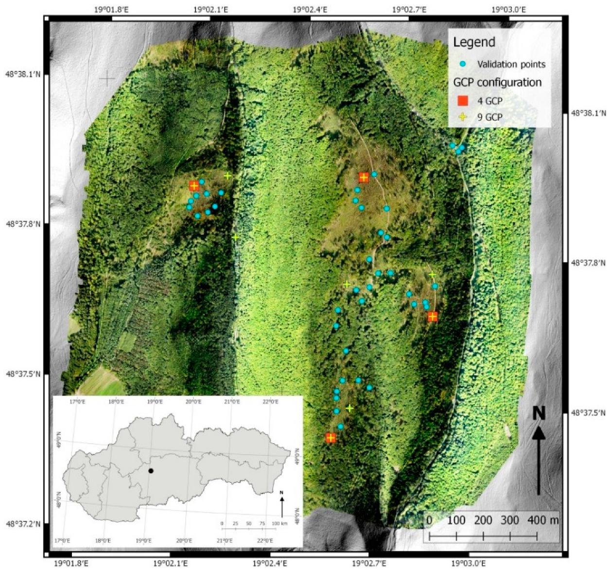
The study area of approximately 270 ha is located near Kašova Lehôtka, Slovakia (~48°37’41”N, 19°02’19”E, Figure 1). The study area is dominated by Fagus sylvatica (L.) and partially covered by Larix decidua (Mill.), Picea abies (L.) and other species. The terrain is rugged, including two valleys and adjacent ridges. Elevation varies from 490 m to 700 m above sea level. Significant portions of the forests were struck by a windthrow disturbance in 2014. At the time of this study, the disturbance impacts were partially recovered and areas radiating away from the disturbance were progressively covered by successional vegetation.

A total of 9 ground control points (GCPs) and 40 validation points (VPs) were established for the UAV accuracy evaluation. GCPs were used only for georeferencing and did not enter final accuracy analyses, where the VPs were used. All points were marked and identified using a cross consisting of two white panels 100 × 15 cm. The shape was chosen to be able to identify the centre even if parts of the cross was unidentifiable in the image. The arms and centre of the crosses were attached to the ground using long nails. The positions of the cross centres (central nail), which served as a reference for all subsequent analyses, were acquired using the GNSS RTK method. We used a survey-grade Topcon Hiper SR receiver (Topcon, Tokyo, Japan) and 20 second intervals as observation period. The differential correction data were acquired using a real-time connection with the Slovak real-time positioning service (SKPOS, http://www.skpos.gku.sk/en/). For a fixed solution, the declared SKPOS accuracy is under four centimetres. All coordinates were acquired using the Slovak national coordinate system S-JTSK (EPSG: 5514), which was also used for all subsequent analyses. Measures were taken to avoid significant shift of the point position between vegetation leaf-off and leaf-on seasons. During the leaf-on measurement, the points were first staked out using positions acquired during the leaf-off measurement. If the cross was still identifiable or at least the central nail was found, we only renewed the crosses. However, in most cases it was necessary to establish a new point and measure its position, because the crosses were destroyed. The average shift between points used in leaf-off and leaf-on seasons was only 0.095 m (SD=0.109 m, max=0.471 m). Therefore, we consider terrain conditions the same.

2.2. UAV Configuration and Acquisition of Photogrammetric Data

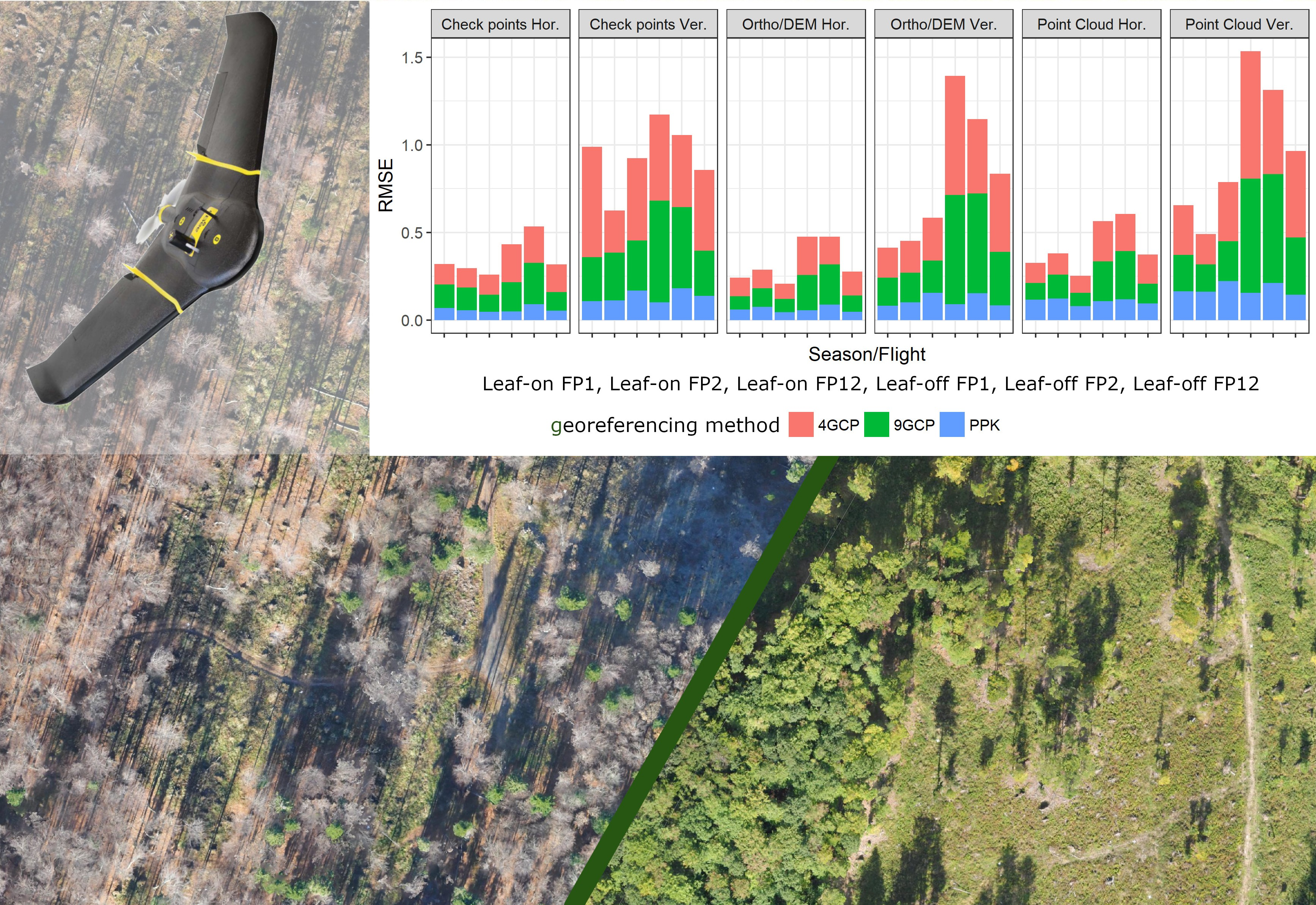
A SenseFly eBee Plus UAV (SenseFly, Cheseaux-sur-Lausanne, Switzerland) with activated GNSS RTK/PPK technology was used. This fixed-wing UAV has a wingspan of 110 cm, weights 1,1 kg and is launched by hand. A SenseFly S.O.D.A. RGB camera was used to obtain the imagery. The 20 megapixel camera mounted on the eBee UAV can provide ground sample distance (GSD) of 2.9cm/pixel at the 120m AGL flight altitude. Focal length is fixed to 10.6 mm (comparable with 29 mm focal length on a 35 mm film camera); aperture is F2.8. Speeds of its global shutter can vary from 1/30 to 1/2000 s. GNSS receiver used in the UAV configuration was the Septentrio AsteRx-m UAS. This dual-channel receiver is capable of tracking L1 and L2 channels of NAVSTAR GPS and GLONASS systems using 132 hardware channels. The manufacturer declares horizontal accuracy of 0.6 cm + 0.5 ppm and vertical accuracy 1 cm + 1 ppm for RTK method.

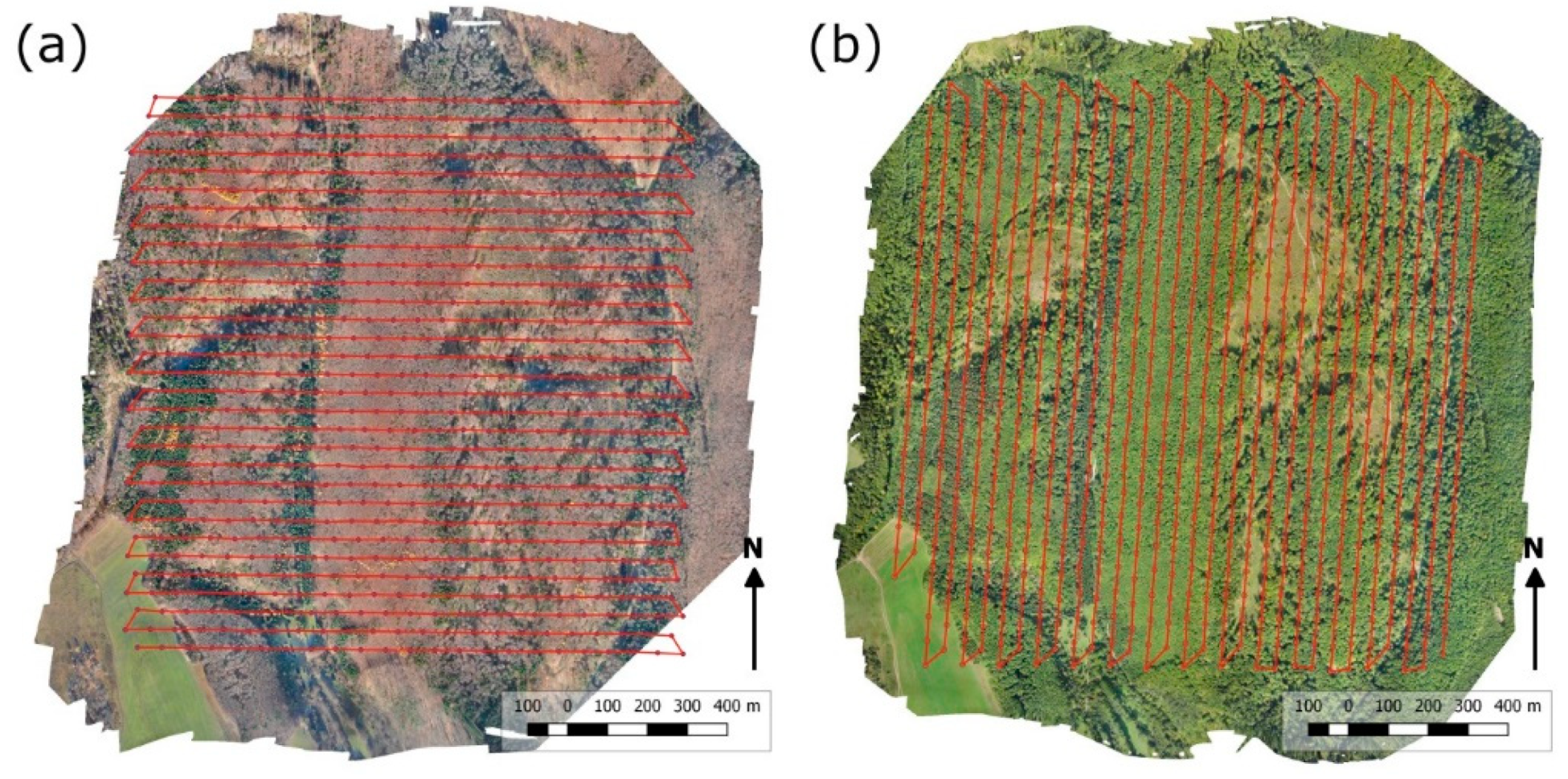
Flights were planned and processed in the eMotion 3 software provided with the UAV. For each photogrammetric campaigns under leaf-off (15 November 2017) and leaf-on (13 September 2018) conditions, two flight patterns were tested (Figure 2). Because the study area is characterized by distinctive valleys and ridges, the first flight pattern (hereinafter referred to as FP1) used rows of images perpendicular to the valleys, while the second flight pattern (FP2) used a direction parallel with the valleys. During the evaluation, these patterns were processed separately, as well as combined, which is hereinafter referred to as the FP12 dataset. The image overlaps were 80x60% in the two dimensions with GSD between 4-5 centimetres from a flight height of 170-180m AGL. A real-time radio connection to a GNSS base is needed for the RTK mode. Instead of this, we used the PPK mode (post-processed kinematic), where raw GNSS data were recorded during the flight and subsequently postprocessed using the differential correction data from the virtual reference station (VRS) data provided by the SKPOS service in the eMotion 3 software. Basic accuracy parameters of the postprocessing are reported in Results. The manufacturer declares the same accuracy (2–3 cm) of camera positioning for both RTK and PPK mode.

2.3. Processing of Photogrametric Data

The images were processed in the Agisoft Photoscan 1.4 software (Agisoft LCC, St. Petersburg, Russia [37]) using the standard workflow. All following steps were done separately, with some differences between the PPK, 4GCP and 9GCP configurations. First, 18 sub-projects were created to allow independent evaluation of all variables and their possible combinations (three georeferencing approaches, two vegetation conditions and three flight patterns). In the case of PPK solution, postprocessed camera positions were attached to EXIF metadata of every geotagged image. For the 4GCP and 9GCP configurations, this information was removed. Images were then aligned using the original resolution. “Reference preselection” was used in the case of the RTK/PPK solution, where the position is used in the first step to acquire a preselected pairs. “Generic preselection” was used for the 4GCP and 9GCP configurations, where the resolution of images was lowered and preselected pairs were made. Then these preselected pairs were aligned. The alignment process was redone for the 4GCP and 9GCP configurations after the 4 and 9 points were placed. After alignment, all validation points were placed for the accuracy calculations. Subsequent steps included generation of dense clouds (High quality), orthomosaics and digital elevation models. Orthomosaics were exported with 5 cm/pixel resolution and DEM with 10 cm resolution.

2.4. Evaluation of Point Cloud and Orthophoto Accuracy

The evaluation of point cloud and orthomosaics accuracy was conducted using 40 validation points.

The accuracy of dense point clouds was evaluated using a point vectorization tool (“Draw Point”) in the Agisoft Photoscan 1.4 software. Points were placed on identified centres of crosses and automatically attached to the nearest point of the point cloud. Resulting point shapefile layers (.shp) were imported into QGIS 2.18 software (open-source software [38]) and subsequently exported as text files with point IDs and X, Y, Z coordinates. These coordinates were compared with the reference positions of the validation points.

The accuracy of the final photogrammetric products - orthomosaics and DEMs were evaluated using QGIS 2.18 software. X and Y coordinates were acquired using a point shapefile layer, where the points represented centres of the crosses clicked after proper identification on the orthophoto raster layer. Z coordinates were subsequently assigned using the 2D coordinates, DEM raster and “Point sampling tool” plugin. Resulting coordinates were exported as a text file and compared to the reference positions of the validation points.

2.5. Statistical Analysis

The coordinates of the 40 validation points, acquired from the original imagery, point clouds and orthophotos were compared to the coordinates in the outputs as follows:

Calculation of the root mean square coordinate errors:

$$RMS{E}_x=\sqrt{\frac{{\sum }_{i=1}^n∆x_i{}^2}{n}}$$

(1)

$$RMS{E}_y=\sqrt{\frac{{\sum }_{i=1}^n∆y_i{}^2}{n}}$$

(2)

$$RMS{E}_z=\sqrt{\frac{{\sum }_{i=1}^n∆z_i{}^2}{n}}$$

(3)

where Δx_i, Δy_i and Δz_i are the differences between reference coordinates and the coordinates determined from the remote sensing data and n is the number of points in the set. Minima, maxima, means and standard deviations were calculated for Δz_i to enable a more detailed analysis of the vertical accuracy. The RMSE_x and RMSE_y errors were used for the calculation of the root mean square horizontal error RMSE_xy as follows:

$$RMS{E}_{xy}=\sqrt{RMS{E}_x{}^2+RMS{E}_y{}^2}$$

(4)

The RMSE_xy is one of the most common horizontal accuracy criteria for sets of points and was used as the main measure to compare data originating in different datasets. Eighteen evaluation variables (groups) were compared for every photogrammetric product, based on georectification approach, vegetation conditions and flight patterns.

Positional error of individual points, Δp—was used to analyse the within-group variability because the RMSE_xy errors do not provide such an information. This error represents a distance between the position of a point acquired on photogrammetric data and the reference position. The error was determined using the following equation:

$$∆p_i=\sqrt{∆x_i{}^2+∆y_i{}^2}$$

(5)

Minima, maxima, means and standard deviations of the positional errors were calculated and used as a base for boxplots depicting variability of differing datasets.

For detection of trends in horizontal and vertical errors, we used three-way factorial ANOVA to investigate the influence of georectification approaches, vegetation conditions and flight patterns. Subsequently, we used Tukey’s post hoc comparison test in R software [39] to determine the significance of differences between the different factors and their levels.

3. Results

3.1. GNSS PPK Solution and Photoscan Software Internal Validation

Most processing software can provide basic measures of achievable accuracies even if validation points are not used to conduct accuracy analyses. However, the procedure for calculating the mean values is not clear in many cases, especially when there is no ground truth data to compare with. The reliability of such values of internal accuracy is limited. In our study, the limited sample size introduces another issue. Direct comparison of RMSEs between datasets, where the mean value is calculated using four (4CGP), nine (9GCP) and >600 values (PPK) would be inappropriate. Therefore, values in this section serve only as a summary of measures provided by software and were not used in subsequent statistical analyses.

Root mean square horizontal and vertical errors for GNSS PPK solution were calculated based on errors of individual camera positions, provided by the post-processing software. Results are presented in

Table 1. Number of camera positions (n), root mean square horizontal and vertical errors in camera positions for GNSS PPK solution (in meters).

	Leaf-off Season		Leaf-on Season
	FP1	FP2	FP1	FP2
n	666	638	711	735
RMSExy	0.024	0.026	0.025	0.023
RMSEz	0.022	0.031	0.027	0.024

.

Horizontal errors are lower than three centimetres in all cases. Just one vertical error exceeded three centimetres. However, these values represent internal accuracy of the post-processed kinematic solution and cannot be directly compared to the RMSEs in the following sections, where validation reference points was used to calculate the errors.

Agisoft Photoscan software provides internal reports for photogrammetric processes conducted. All reports (including depiction of dense point clouds, time needed for particular evaluation steps and other detailed data) are available as Supplementary Data. Number of cameras (total/aligned), point counts for sparse and dense point clouds, reprojection errors, recalculated GSD and errors of GCPs and camera locations for all evaluation variants are reported in

Table 2. Results of photogrammetric processing for different vegetation conditions, flight patterns and GCP configurations.

				Point Count					Errors 1 (m)
	Flight Pattern	Georecti-Fication Method	Cameras Total/Aligned	Tie Points (thous.)	Dense Cloud (mill.)	Reprojection Error (pixel)	GSD Recalculated (cm)		RMSEH	RMSEV
Leaf-off season	FP1	4GCP	666/629 (94%)	314	170	1.40	6.08		0.156	0.206
		9GCP	666/629 (94%)	316	170	1.40	6.08		0.175	0.416
		PPK	666/631 (95%)	317	202	1.41	6.00		0.0031	0.0061
	FP2	4GCP	638/596 (93%)	306	169	1.21	5.75		0.186	0.447
		9GCP	638/596 (93%)	306	168	1.21	5.75		0.163	0.293
		PPK	638/603 (95%)	308	207	1.24	5.66		0.0051	0.0101
	FP12	4GCP	1304/1234 (95%)	619	220	1.38	5.90		0.127	0.025
		9GCP	1304/1225 (94%)	620	220	1.37	5.90		0.109	0.264
		PPK	1304/1238 (95%)	621	250	1.39	5.82		0.0031	0.0081
Leaf-on season	FP1	4GCP	711/711 (100%)	647	304	1.47	5.99		0.119	0.101
		9GCP	711/711 (100%)	648	311	1.46	5.94		0.116	0.188
		PPK	711/711 (100%)	645	312	1.48	5.95		0.0041	0.0091
	FP2	4GCP	735/734 (100%)	522	329	1.41	5.49		0.138	0.168
		9GCP	735/734 (100%)	524	349	1.41	5.43		0.126	0.188
		PPK	735/735 (100%)	521	348	1.42	5.43		0.0051	0.0091
	FP12	4GCP	1446/1446 (100%)	1172	372	1.51	5.74		0.062	0.039
		9GCP	1446/1446 (100%)	1172	380	1.50	5.68		0.081	0.136
		PPK	1446/1446 (100%)	1173	380	1.51	5.69		0.0031	0.0081

¹ For PPK, average camera location errors are reported instead of horizontal and vertical errors on GCPs.

.

Substantial differences between leaf-off and leaf-on conditions can be seen already in the camera alignment. In the leaf-on season, almost all cameras were successfully aligned, whereas in leaf-off season there are cameras which were not aligned (up to 7%). Horizontal errors around the GCPs range from 6.21 to 18.6 cm. Variability of vertical errors is even higher—from 3.93 to 44.7 cm. Errors of camera locations, reported for the PPK solution, are under one centimetre. However, the average camera location errors of the PPK method cannot be compared to results of the GCP approaches due to much higher number of values (>600 versus 4 or 9) entering the calculation as well as lack of the ground truth. The average camera location errors are the only accuracy measure, when no GCPs and CPs are used Overall, we consider this value unreliable for estimation of actual accuracy.

3.2. Accuracy using the Validation Points in Photoscan

Accuracy achieved on validation points in Agisoft Photoscan 1.4 software can be considered one of the earliest accuracy measures during the photogrammetric processing. Points were identified on multiple original images after their alignment. Horizontal and vertical root mean square errors of positions of points for this kind of evaluation are reported in

Table 3. Horizontal root mean square errors (RMSE_xy) of validation points used in Photoscan software (in meters).

		Leaf-off Season			Leaf-on Season
		FP1	FP2	FP12	FP1	FP2	FP12
Georec. method	4GCP	0.215	0.208	0.159	0.282	0.111	0.114
	9GCP	0.167	0.236	0.106	0.135	0.131	0.098
	PPK	0.049	0.089	0.053	0.068	0.054	0.047

and

Table 4. Vertical root mean square errors (RMSE_z) of validation points used in Photoscan software (in meters).

		Leaf-off Season			Leaf-on Season
		FP1	FP2	FP12	FP1	FP2	FP12
Georec. method	4GCP	0.489	0.411	0.459	0.629	0.239	0.470
	9GCP	0.581	0.464	0.258	0.252	0.273	0.284
	PPK	0.100	0.18	0.138	0.107	0.111	0.168

.

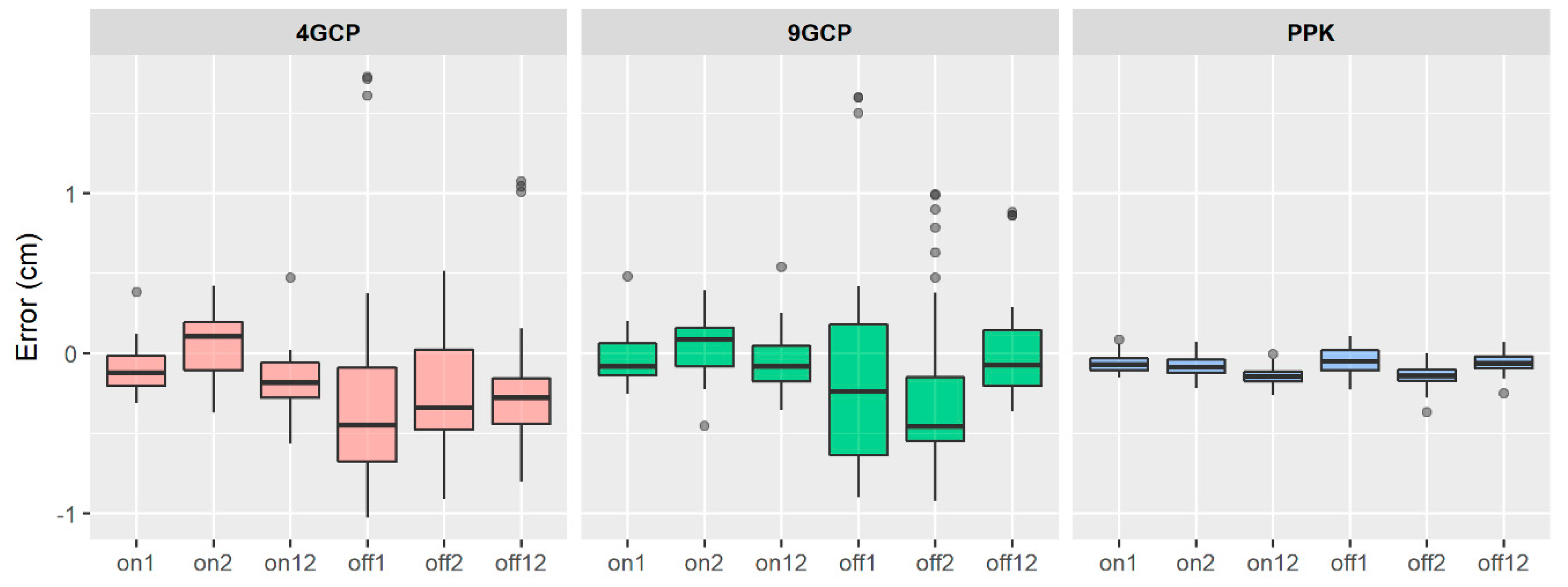
Both horizontal and vertical errors of the PPK solution are lower than those acquired using GCPs. Horizontal errors for PPK were up to 10 centimetres, while vertical errors did not reach 20 cm. The highest horizontal error for GCP solution is 28.2 cm; the highest vertical error is 58.1cm. The variability of horizontal errors is higher when GCPs are used (Figure 3). A similar pattern is observed in the vertical errors but mainly within the leaf-off season (Figure 4).

3.3. Point Cloud Accuracy

In terms of SfM photogrammetric processing, point clouds were a sub-step between original imagery and final products—i.e., orthophotos and DEMs. However, point cloud applications are increasingly common due to their comparability, for example, to laser point clouds. Therefore, the evaluation of point cloud accuracy was conducted. Horizontal and vertical root mean square errors of positions of points are reported in

Table 5. Horizontal root mean square errors (RMSE_xy) for point positions in the point clouds (in meters).

		Leaf-off Season			Leaf-on Season
		FP1	FP2	FP12	FP1	FP2	FP12
Georec. method	4GCP	0.231	0.212	0.166	0.114	0.121	0.097
	9GCP	0.226	0.273	0.113	0.096	0.137	0.078
	PPK	0.108	0.119	0.095	0.115	0.122	0.078

and

Table 6. Vertical root mean square errors (RMSE_z) for point positions acquired on point clouds (in meters).

		Leaf-off Season			Leaf-on Season
		FP1	FP2	FP12	FP1	FP2	FP12
Georec. method	4GCP	0.726	0.481	0.495	0.285	0.173	0.337
	9GCP	0.651	0.619	0.327	0.207	0.156	0.228
	PPK	0.155	0.212	0.143	0.164	0.161	0.222

.

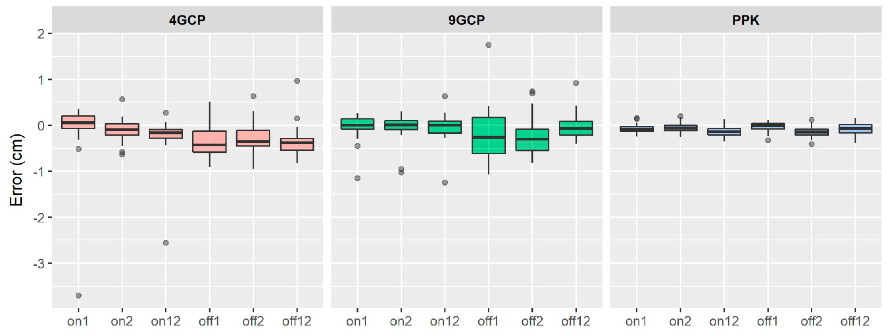
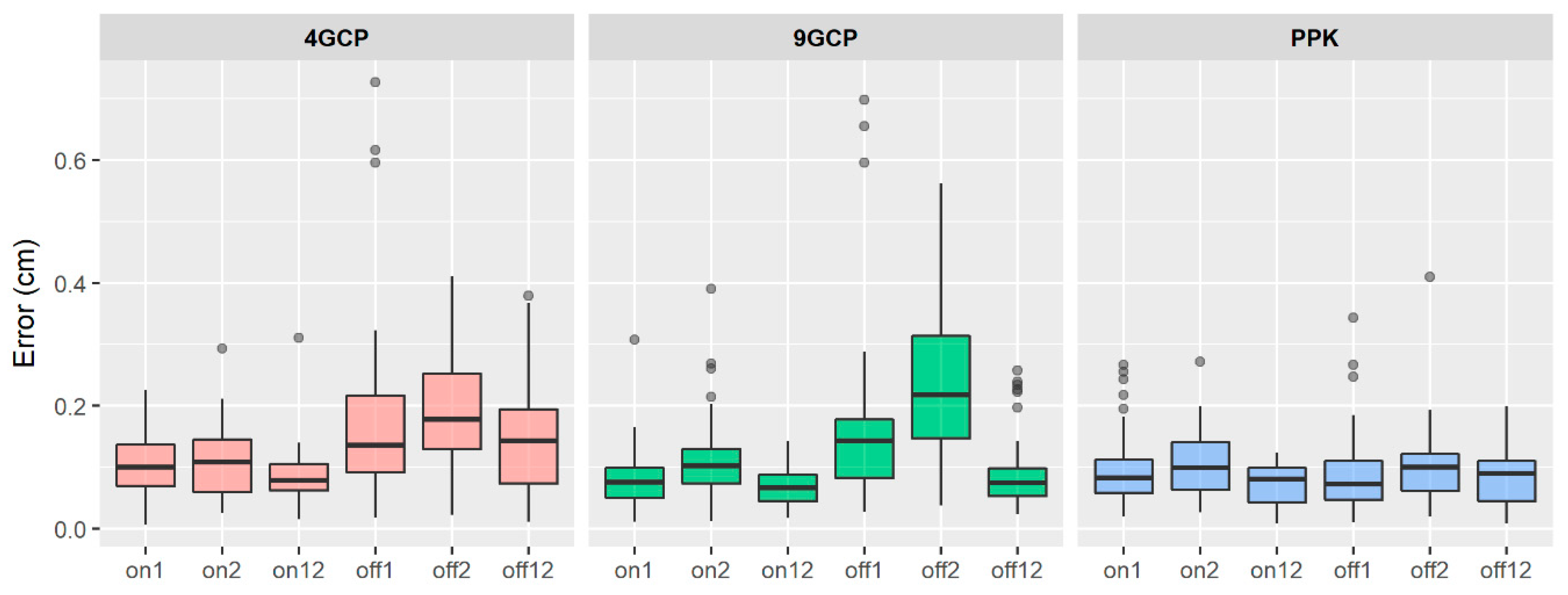
In most cases, the errors were higher than those for the validation points identified in the original imagery. This can be, to some degree, caused by complications related to the identification of points on a relatively sparse point clouds (in appropriate level of zoom). Variability of results especially in the leaf-on season is lower; errors of GCP solutions are closer, in some cases even lower, to errors of the PPK solution (Figure 5 and Figure 6).

3.4. Orthomosaic and DEM Accuracy

Horizontal accuracy of the final orthomosaic was evaluated using the QGIS software by vectorization of the centres of the crosses. Z coordinates were subsequently acquired using point sampling from digital elevation model. Horizontal and vertical root mean square errors are presented in

Table 7. Horizontal root mean square errors (RMSE_xy) for point positions in the orthomosaic (in meters).

		Leaf-off Season			Leaf-on Season
		FP1	FP2	FP12	FP1	FP2	FP12
Georec. method	4GCP	0.218	0.158	0.138	0.106	0.106	0.087
	9GCP	0.201	0.229	0.092	0.075	0.107	0.076
	PPK	0.055	0.087	0.047	0.059	0.074	0.044

and

Table 8. Vertical root mean square errors (RMSE_z) for point positions acquired on digital elevation models (in meters).

		Leaf-off Season			Leaf-on Season
		FP1	FP2	FP12	FP1	FP2	FP12
Georec. method	4GCP	0.679	0.423	0.446	0.172	0.181	0.245
	9GCP	0.623	0.569	0.305	0.159	0.169	0.185
	PPK	0.089	0.154	0.084	0.082	0.101	0.154

.

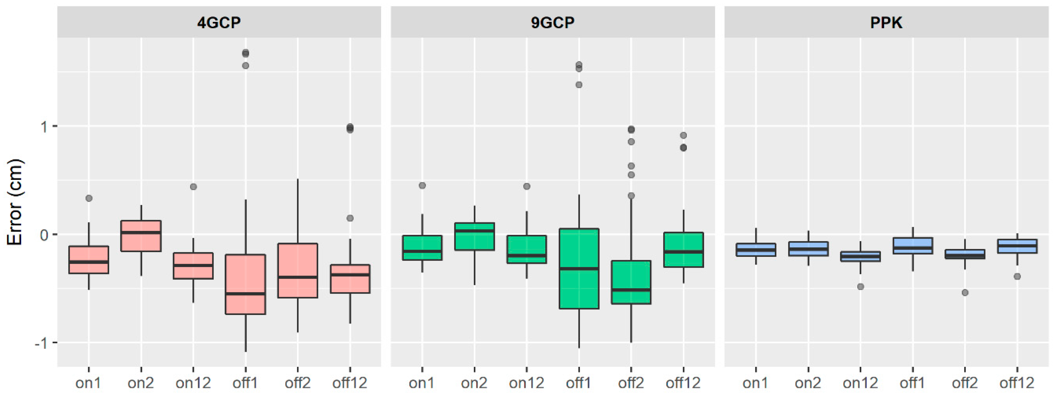
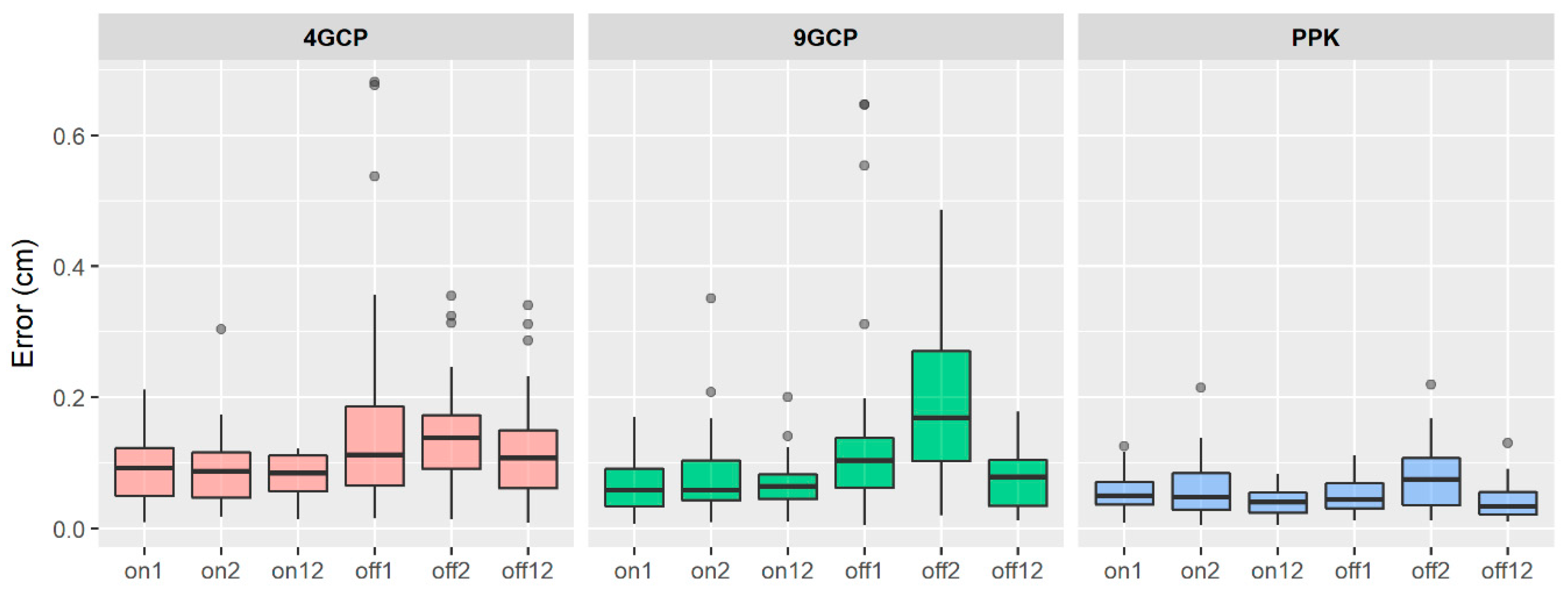
Overall, errors were lower when compared to the errors in the point clouds. Horizontal errors of the PPK solution did not exceed 10 centimetres. The same applies to results of the combined flight pattern (FP12), except one case (13.8 cm). Errors of the GCP solutions are lower in the leaf-on season. In the leaf-off season, three vertical errors exceeded 50 cm, all related to the GCP solution. For these cases also the variability is greater when compared to others (Figure 7 and Figure 8). The PPK has lower variability in all cases.

3.5. Comparison of Root Mean Square Errors

Most accurate results, as demonstrated by the RMSEs, were achieved by the PPK method across all approaches. From the histogram (Figure 9), larger differences in vertical accuracy can be observed between seasons, when 4GCP and 9GCP were used (especially for vertical accuracy), whereas leaf-on is more accurate.

3.6. Factors Influencing Accuracy

The influence of main factors on the horizontal and vertical accuracies was analysed using a factorial ANOVA. For the horizontal accuracy, ANOVA results (

Table 9. Results of the three way factorial ANOVA for horizontal accuracy. Evaluated factors: georectification method (GCP), flight pattern, vegetation season; and their interactions.

Factor (Interaction)	Degrees of Freedom	Sum Squared	Mean Squared	F Value	Pr(>F)
GCP	2	0.582	0.29106	55.198	< 0.0000
Season	1	0.263	0.26312	49.900	< 0.0000
Flights	2	0.179	0.08960	16.992	< 0.0000
GCP:Season	2	0.137	0.06849	12.988	< 0.0000
GCP:Flights	4	0.083	0.02084	3.951	0.00352
Season:Flights	2	0.053	0.02629	4.986	0.00707
GCP:Season:Flights	4	0.058	0.01448	2.746	0.02752
Residuals	724	3.818	0.00527

140 observations deleted due to missingness.

) show a statistically significant difference in the mean error for all factors and their interactions (factors: flight patterns, GCP patterns and vegetation seasons). The combined flight pattern FP12 is statistically different from the patterns where only one direction was used. In the case of georectification methods, the PPK method is statistically different from both 4GCP and 9GCP method. Also the vegetation seasons are statistically different from each other. Furthermore, from the interactions GCP:Season, GCP:Flights, Season:Flights and GCP:Season:Flights, it can be observed that the PPK method in leaf-on season and FP12 flight pattern are providing significantly higher accuracy compared with all other levels of factors. Moreover, the accuracy of PPK method is not influenced by season like the 4GCP and 9GCP configurations are.

Subsequently, the influence of above mentioned factors was tested for vertical accuracy. A statistically significant difference can be observed for GCP patterns, seasons and following interactions GCP:Season, GCP:Flights, Season:Flights (

Table 10. Results of the three way factorial ANOVA for vertical accuracy. Evaluated factors: georectification method (GCP), flight pattern, vegetation season; and their interactions.

Factor (Interaction)	Degrees of Freedom	Sum Squared	Mean Squared	F Value	Pr(>F)
GCP	2	1.37	0.6872	7.714	0.00048
Season	1	1.62	1.6210	18.196	0.00002
Flights	2	0.00	0.0024	0.027	0.97378
GCP:Season	2	1.36	0.6793	7.625	0.00053
GCP:Flights	4	0.87	0.2179	2.446	0.04519
Season:Flights	2	1.76	0.8792	9.870	0.00006
GCP:Season:Flights	4	0.19	0.0476	0.535	0.71040
Residuals	724	64.50	0.0891

140 observations deleted due to missingness.

). On the other hand, influence of flight patterns and the three-way interaction are not statistically significant. The Tukey post hoc test (Supplementary Data) indicated that the vertical accuracy is not influenced by flight patterns in general. PPK method is significantly different from 4GCP (leaf-off season) and from 9GCP (leaf-on season). Other important result is that the vertical accuracy of PPK method is not influenced by seasons when the 4GCP and 9GCP are.

In general, the vertical and horizontal accuracy (RMSEs) was better for the PPK method when compared to 4GCP and 9GCP variants (Figure 9). Most importantly, the PPK accuracy is not influenced by season and in the case of horizontal accuracy also by flights patterns.

4. Discussion

Overall, influence of GCP numbers and spatial distribution have been widely studied but conclusions often differ significantly. In terms of accuracy assessment and GCP configuration, this study partially follows our previous study [40], where we reported RMSE_xy from 0.04 m to 0.11 m for the 4GCP pattern, while RMSEs of the 9GCP pattern were from 0.04 m to 0.08 m. However, the DJI Phantom 3 UAV was used at significantly lower flight altitudes (50–60 m) and the test plot areas were smaller. Vertical RMSEs were in range from 0.08 to 0.17 m. Aguera-Vega et al. [41] studied influence of GCP count (4–20 GCPs) and pattern on a ~18 ha plot and achieved the best accuracy with 15 GCP. They declare wide range of slope values; the elevation range was about 60 m. For smaller areas (2.8–4.1 ha), He et al. [42] used 9–10 GCPs and achieved horizontal RMSEs of 1–3 centimetres and vertical RMSE of 4 centimetres. The authors designed an algorithm to improve accuracy of automated aerial triangulation, however, the height of flight was significantly lower—40 to 60m. Fewer studies were conducted on areas larger than 100 ha. Rangel et al. [43] used multiple flights of a S500 multicopter and studied differing GCP configurations on an area of 400 ha. They did not find any significant increase of orthophoto accuracy when the GCP count was over 18. Tahar [44] conducted a photogrammetric survey of a 150 ha area using 4–9 GCPs and achieved an RMSE_xy of 0.50 m and RMSE_z of 0.78 m. Küng et al. [45] used 19 GCPs on an area of 210 ha and reported horizontal accuracy of 0.38 m and vertical accuracy of 1.07 m for a flight height of 262 m AGL.

In terms of accuracy, increasing number of GCPs and their regular spatial distribution has a positive effect. However, from practical point of view, a simple increase of GCP number makes the survey more labour intensive and less effective. This is particularly evident in forests where the use of GNSS for GCP measurements is complicated. In such cases (but not limited to these), RTK/PPK technology applied with UAVs can be a feasible solution. Tests of this technology outside forest ecosystems have already been conducted. Gerke and Przybilla [46] tested the technology on an stockpile area. For this 1100 × 600 m area with 50 m maximum height difference, they achieved horizontal and vertical RMSEs under 10cm. Another result of this test was that addition of GCPs did not provide better accuracy when the RTK technology was enabled. Benassi et al. [47] used a senseFly eBee RTK UAV to test the accuracy at a 400 × 500 m area comprising of a part of a university campus with buildings up to 35 m height. On 14 checkpoints, they achieved average horizontal RMSE of 2.2 cm for differing software packages. The elevation accuracy was more than two times worse; authors suggest application of at least one GCP to gain control over the biases influencing elevation. Another test of the UAV RTK solution was conducted on 80 ha area with flat terrain and buildings [48]. Reported horizontal RMSEs were under four centimetres for both real-time and post-processed variants of GNSS measurement. However, in this case authors suggest that “classical” aerotriangulation with GCPs is better than the direct georeferencing. Achievable accuracy of the RTK/PPK therefore seems higher than the one achieved in our study, however, our results are related to much more complicated terrain conditions. When comparing RTK/PPK georeferencing approach to georeferencing with the use of GCPs, significantly higher number of precise positions entering the bundle adjustment must be also considered. The number for PPK solution in our study was higher than 600, while only four and nine GCPs were used for our configurations.

The influence of flight patterns on the achieved accuracy was tested in multiple studies. In our case, the patterns were adapted to the main terrain lines (valleys, ridges). Despite this design, the influence of flight patterns on the vertical accuracy was not confirmed. The differences of horizontal accuracy for individual flight patterns FP1 and FP2 were not significant but the combined FP12 pattern provided significantly better accuracy compared to both of them. This effect of combined patterns, often referred to as crossflights, is described for example, by Manfreda et al. [49]. Six flight patterns, some with tilted camera, were used to achieve higher accuracy. Authors report the combination of patterns as the most accurate, in terms of both horizontal and vertical accuracy. Increased influence of crossflights with decreasing number of GCPs is reported in another study [46]. Authors also report a non-substantial but visible increase of accuracy for the RTK UAV technology when employed with cross-flights. A practical problem of the combined patterns is the increased amount of redundant data. This can induce problems especially in more complex projects, where the computational power needed to process the data can be very high.

The significant negative impact of the leaf-off season already during alignment of imagery can limit possibilities of constructing digital terrain models from UAV imagery. The limited ability to reconstruct terrain under full forest canopy is one of the main disadvantages of SfM when comparing photogrammetry with LiDAR. However, multiple studies reported some success during the leaf-off season or under partially opened canopy. Graham et al. [50] reconstructed up to 60% of terrain with an RMSE lower than 1.5m in disturbed conifer forest. Guerra-Hernández et al. [12] studied terrain under a Eucalyptus plantation with canopy cover higher than 60% and reported terrain height overestimation over two meters. Moudrý et al. [51] mapped a post-mining site under leaf-off conditions and achieved point cloud accuracy between 0.11 and 0.19 m. Similar team of authors [52] reported a DTM acquired in forest during the leaf-off season as the most accurate when compared with aquatic vegetation and steppe ecosystems. Through application of the Best Available Pixel Compositing (BATP) on multi-temporal UAV imagery, Goodbody et al. [53] were able to obtain DTMs with a 0.01 m mean error, a standard deviation of 0.14m and a relative coverage of 86.3% compared with the reference DTM. The stem density was relatively low (50 stems/ha). The authors suggest that the imagery acquisition timing has a significant impact on DTM error with assumption that the acquisition in spring, late-fall and early winter was the most accurate. This is in contrast with our results. We explain this by a monotone pattern of mostly monocultural, fully-stocked Beech forests during the leaf-off season. This lack of distinctive features resulted into failure of image alignment on parts with continuous forest. During the leaf-on season, the crowns of the trees and gaps between them provided sufficient background for the alignment.

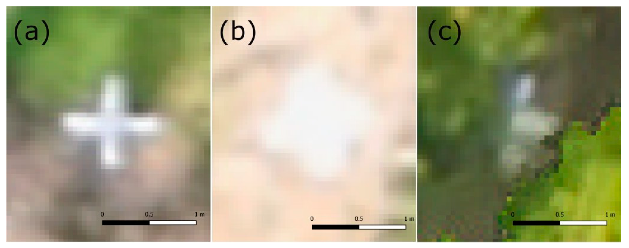
Besides the actual accuracy, the ability to identify points of interest can significantly influence results of photogrammetric evaluation. The process of point identification demands some operator’s experience with image interpretation, especially when interpreting natural features [54]. Even though points in our study were identified using crosses, we have observed some difficulties during the identification on point clouds and orthomosaics (Figure 10). Slightly shaded conditions were ideal, where the shape and dimensions of the crosses were clearly distinguishable. In contrast, sharply illuminated bright surfaces caused deformation of the pixels and their spectra during the process of orthorectification. Special cases were related to the vegetation canopy boundaries. The identification of the point centres was even more complicated in the point clouds. Despite the total point count of hundreds of millions points, the point clouds were too sparse to properly zoom in on the point centre. We consider this the reason of lower accuracy when comparing point clouds to orthophotos.

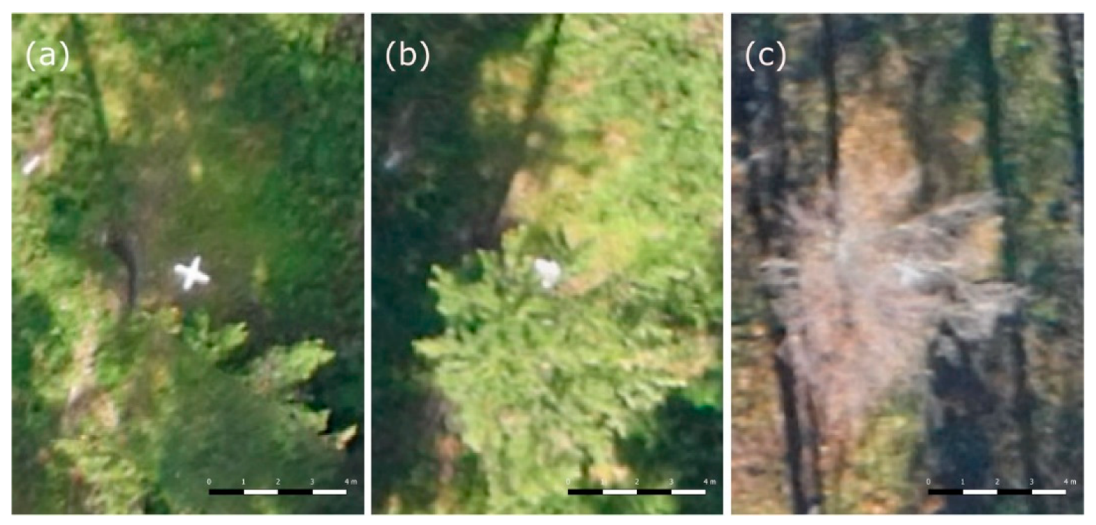
During the orthophoto evaluation, we experienced difficulties with identification of particular points at the edges of forest stands. In some cases, trees were rendered over such points on the orthophoto, even when the points were situated outside the canopy during the field survey. This is because the product used is a standard orthophoto, not a “true orthophoto” [55,56]. This can be seen when the flight pattern is perpendicular to the edge of the forest (Figure 11). As the identification of forest gaps is a frequent task in forestry (e.g., [23,24]), this can introduce errors, especially when the desired accuracy is high. Agisoft Photoscan software allows editing the seamlines and thus production of true orthophotos but the labour intensity is increased significantly. In contrast with evaluation of the orthophotos, the use of point clouds allowed non-problematic identification of points partially occluded by trees. However, in few cases the point was snapped to a point belonging to the tree instead of ground.

Overall, the RTK/PPK solution used in this study could be suitable for mapping inaccessible areas if the desired horizontal error is lower than 10 cm and vertical error is under 20 cm. Besides the accuracy, other practical challenges must be considered, if the technology is to be applied effectively. For example, if the possible flight time of the platform is short or the UAV must operate within a line-of-sight of an operator, the feasibility for mapping inaccessible or hazardous areas is significantly limited. But UAVs with—one hour flight time can reach more distant areas, thus, in combination with the RTK/PPK technology, can provide the remote sensing independent on terrestrial measurements. Higher initial costs must also be considered. In case of eBee UAVs, the cost of the RTK/PPK technology is in range of several thousands of Euros (compared to the UAV without the RTK/PPK technology). However, utilization of GCPs also requires a GNSS receiver and its price must be considered.

5. Conclusions

We test the capability of the UAV RTK/PPK and demonstrate highly accurate spatial data comparable with data acquired using standard referencing approaches (GCPs). Additional factors with a supposedly significant influence on accuracy were also evaluated. More specifically we have investigated the impact of vegetation season, flight patterns and processing methods. The results of the RTK/PPK method were clearly more accurate and less prone to influence of these factors when compared to the GCP approaches. Increasing the number of GCPs would probably lead to increases in accuracy but such an approach is undesirable in inaccessible and hazardous areas.

In most cases horizontal RMSEs of the RTK/PPK method did not exceed 10 cm and vertical RMSEs were under 20 cm. Slightly less accurate results were achieved on the point clouds (compared to the original imagery after alignment and orthophotos, DEMs). This was most probably caused by limited possibility to identify point centres on this data. The results suggest that the RTK/PPK method can provide data with comparable or even higher accuracy compared to the GCP approaches, independently on the terrestrial measurements. This is the main requirement for remote sensing of inaccessible and hazardous areas in forests (but not limited to them). If the principal question was whether the RTK/PPK method can be the optimal solution of mapping such areas, the answer could be: Yes. However, besides further testing of accuracy ambiguities, also the technical parameters of UAVs (maximum flight time, autonomous operation etc.) must be adjusted to fully gain the benefits of these possibilities.

References

- Piermattei, L.; Marty, M.; Karel, W.; Ressl, C.; Hollaus, M.; Ginzler, C.; Pfeifer, N. Impact of the acquisition geometry of very high-resolution Pléiades imagery on the accuracy of canopy height models over forested alpine regions. Remote Sens. 2018, 10, 1542. [Google Scholar] [CrossRef]
- Elatawneh, A.; Wallner, A.; Manakos, I.; Schneider, T.; Knoke, T. Forest cover database updates using multi-seasonal rapideye data-storm event assessment in the Bavarian Forest National Park. Forests 2014, 5, 1284–1303. [Google Scholar] [CrossRef]
- Persson, H.J. Estimation of boreal forest attributes from very high resolution pléiades data. Remote Sens. 2016, 8, 736. [Google Scholar] [CrossRef]
- Matasci, G.; Hermosilla, T.; Wulder, M.A.; White, J.C.; Coops, N.C.; Hobart, G.W.; Zald, H.S.J. Large-area mapping of Canadian boreal forest cover, height, biomass and other structural attributes using Landsat composites and lidar plots. Remote Sens. Environ. 2018, 209, 90–106. [Google Scholar] [CrossRef]
- Lee, W.-J.; Lee, C.-W. Forest Canopy Height Estimation Using Multiplatform Remote Sensing Dataset. J. Sens. 2018, 2018, 1593129. [Google Scholar]
- Simard, M.; Pinto, N.; Fisher, J.B.; Baccini, A. Mapping forest canopy height globally with spaceborne lidar. J. Geophys. Res. Biogeosci. 2011, 116, 1–12. [Google Scholar] [CrossRef]
- Pourrahmati, M.R.; Baghdadi, N.; Darvishsefat, A.A.; Namiranian, M.; Gond, V.; Bailly, J.S.; Zargham, N. Mapping lorey’s height over Hyrcanian forests of Iran using synergy of ICESat/GLAS and optical images. Eur. J. Remote Sens. 2018, 51, 100–115. [Google Scholar] [CrossRef]
- Chen, H.; Cloude, S.R.; Goodenough, D.G. Forest Canopy Height Estimation Using Tandem-X Coherence Data. IEEE J. Sel. Top. Appl. Earth Obs. Remote Sens. 2016, 9, 3177–3188. [Google Scholar] [CrossRef]
- García, M.; Saatchi, S.; Ustin, S.; Balzter, H. Modelling forest canopy height by integrating airborne LiDAR samples with satellite Radar and multispectral imagery. Int. J. Appl. Earth Obs. Geoinf. 2018, 66, 159–173. [Google Scholar] [CrossRef]
- Carvalho-Santos, C.; Monteiro, A.; Arenas-Castro, S.; Greifeneder, F.; Marcos, B.; Portela, A.; Honrado, J. Ecosystem Services in a Protected Mountain Range of Portugal: Satellite-Based Products for State and Trend Analysis. Remote Sens. 2018, 10, 1573. [Google Scholar] [CrossRef]
- Mohan, M.; Silva, C.A.; Klauberg, C.; Jat, P.; Catts, G.; Cardil, A.; Hudak, A.T.; Dia, M. Individual tree detection from unmanned aerial vehicle (UAV) derived canopy height model in an open canopy mixed conifer forest. Forests 2017, 8, 340. [Google Scholar] [CrossRef]
- Guerra-Hernández, J.; Cosenza, D.N.; Rodriguez, L.C.E.; Silva, M.; Tomé, M.; Díaz-Varela, R.A.; González-Ferreiro, E. Comparison of ALS- and UAV(SfM)-derived high-density point clouds for individual tree detection in Eucalyptus plantations. Int. J. Remote Sens. 2018, 39, 5211–5235. [Google Scholar] [CrossRef]
- Hentz, Â.M.K.; Silva, C.A.; Dalla Corte, A.P.; Netto, S.P.; Strager, M.P.; Klauberg, C. Estimating forest uniformity in Eucalyptus spp. and Pinus taeda L. stands using field measurements and structure from motion point clouds generated from unmanned aerial vehicle (UAV) data collection. For. Syst. 2018, 27, e005. [Google Scholar] [CrossRef]
- Guerra-Hernández, J.; González-Ferreiro, E.; Monleón, V.J.; Faias, S.P.; Tomé, M.; Díaz-Varela, R.A. Use of multi-temporal UAV-derived imagery for estimating individual tree growth in Pinus pinea stands. Forests 2017, 8, 300. [Google Scholar] [CrossRef]
- Kayitakire, F.; Hamel, C.; Defourny, P. Retrieving forest structure variables based on image texture analysis and IKONOS-2 imagery. Remote Sens. Environ. 2006, 102, 390–401. [Google Scholar] [CrossRef]
- Neigh, C.; Masek, J.; Bourget, P.; Cook, B.; Huang, C.; Rishmawi, K.; Zhao, F.; Neigh, C.S.R.; Masek, J.G.; Bourget, P.; et al. Deciphering the Precision of Stereo IKONOS Canopy Height Models for US Forests with G-LiHT Airborne LiDAR. Remote Sens. 2014, 6, 1762–1782. [Google Scholar] [CrossRef] [Green Version]
- Honkavaara, E.; Ahokas, E.; Hyyppä, J.; Jaakkola, J.; Kaartinen, H.; Kuittinen, R.; Markelin, L.; Nurminen, K. Geometric test field calibration of digital photogrammetric sensors. ISPRS J. Photogramm. Remote Sens. 2006, 60, 387–399. [Google Scholar] [CrossRef]
- Wallace, L.; Lucieer, A.; Watson, C.; Turner, D. Development of a UAV-LiDAR system with application to forest inventory. Remote Sens. 2012, 4, 1519–1543. [Google Scholar] [CrossRef]
- Puliti, S.; Ørka, H.; Gobakken, T.; Næsset, E. Inventory of Small Forest Areas Using an Unmanned Aerial System. Remote Sens. 2015, 7, 9632–9654. [Google Scholar] [CrossRef] [Green Version]
- Mikita, T.; Janata, P.; Surový, P. Forest stand inventory based on combined aerial and terrestrial close-range photogrammetry. Forests 2016, 7, 165. [Google Scholar] [CrossRef]
- Feduck, C.; McDermid, G.J.; Castilla, G. Detection of coniferous seedlings in UAV imagery. Forests 2018, 9, 432. [Google Scholar] [CrossRef]
- Miller, E.; Dandois, J.P.; Detto, M.; Hall, J.S. Drones as a tool for monoculture plantation assessment in the steepland tropics. Forests 2017, 8, 168. [Google Scholar] [CrossRef]
- Getzin, S.; Nuske, R.S.; Wiegand, K. Using unmanned aerial vehicles (UAV) to quantify spatial gap patterns in forests. Remote Sens. 2014, 6, 6988–7004. [Google Scholar] [CrossRef]
- Bagaram, M.; Giuliarelli, D.; Chirici, G.; Giannetti, F.; Barbati, A.; Bagaram, M.B.; Giuliarelli, D.; Chirici, G.; Giannetti, F.; Barbati, A. UAV Remote Sensing for Biodiversity Monitoring: Are Forest Canopy Gaps Good Covariates? Remote Sens. 2018, 10, 1397. [Google Scholar]
- Puliti, S.; Talbot, B.; Astrup, R. Tree-Stump Detection, Segmentation, Classification and Measurement Using Unmanned Aerial Vehicle (UAV) Imagery. Forests 2018, 9, 102. [Google Scholar] [CrossRef]
- Näsi, R.; Honkavaara, E.; Blomqvist, M.; Lyytikäinen-Saarenmaa, P.; Hakala, T.; Viljanen, N.; Kantola, T.; Holopainen, M. Remote sensing of bark beetle damage in urban forests at individual tree level using a novel hyperspectral camera from UAV and aircraft. Urban For. Urban Green. 2018, 30, 72–83. [Google Scholar] [CrossRef]
- Aasen, H.; Honkavaara, E.; Lucieer, A.; Zarco-Tejada, P.J. Quantitative remote sensing at ultra-high resolution with UAV spectroscopy: A review of sensor technology, measurement procedures and data correctionworkflows. Remote Sens. 2018, 10, 1091. [Google Scholar] [CrossRef]
- Brovkina, O.; Cienciala, E.; Surový, P.; Janata, P. Unmanned aerial vehicles (UAV) for assessment of qualitative classification of Norway spruce in temperate forest stands. Geo-spatial Inf. Sci. 2018, 5020, 1–9. [Google Scholar] [CrossRef]
- Minařík, R.; Langhammer, J. Use of a multispectral UAV photogrammetry for detection and tracking of forest disturbance dynamics. Int. Arch. Photogramm. Remote Sens. Spat. Inf. Sci. ISPRS Arch. 2016, 41, 711–718. [Google Scholar] [CrossRef]
- Wieser, M.; Mandlburger, G.; Hollaus, M.; Otepka, J.; Glira, P.; Pfeifer, N. A Case Study of UAS Borne Laser Scanning for Measurement of Tree Stem Diameter. Remote Sens. 2017, 9, 1154. [Google Scholar] [CrossRef]
- Brede, B.; Lau, A.; Bartholomeus, H.M.; Kooistra, L. Comparing RIEGL RiCOPTER UAV LiDAR derived canopy height and DBH with terrestrial LiDAR. Sensors (Switz.) 2017, 17, 2371. [Google Scholar] [CrossRef] [PubMed]
- Sofonia, J.J.; Phinn, S.; Roelfsema, C.; Kendoul, F.; Rist, Y. Modelling the effects of fundamental UAV flight parameters on LiDAR point clouds to facilitate objectives-based planning. ISPRS J. Photogramm. Remote Sens. 2019, 149, 105–118. [Google Scholar] [CrossRef]
- Westoby, M.J.; Brasington, J.; Glasser, N.F.; Hambrey, M.J.; Reynolds, J.M. “Structure-from-Motion” photogrammetry: A low-cost, effective tool for geoscience applications. Geomorphology 2012, 179, 300–314. [Google Scholar] [CrossRef]
- Hofmann-Wellenhof, B.; Lichtenegger, H.; Wasle, E. GNSS–Global Navigation Satellite Systems: GPS, GLONASS, Galileo and More; Springer Science & Business Media: New York, NY, USA, 2007; ISBN 3211730176. [Google Scholar]
- Ucar, Z.; Bettinger, P.; Weaver, S.; Merry, K.L.; Faw, K. Dynamic accuracy of recreation-grade GPS receivers in oak-hickory forests. Forestry 2014, 87, 504–511. [Google Scholar] [CrossRef] [Green Version]
- Zimbelman, E.G.; Keefe, R.F. Real-time positioning in logging: Effects of forest stand characteristics, topography and line-of-sight obstructions on GNSS-RF transponder accuracy and radio signal propagation. PLoS ONE 2018, 13, e0191017. [Google Scholar] [CrossRef]
- AgiSoft PhotoScan Professional. Software. Version 1.4.6. 2018. Available online: http://www.agisoft.com/downloads/installer/ (accessed on 15 February 2019).
- QGIS Development Team QGIS Geographic Information System. Open Source Geospatial Foundation Project. 2018. Available online: http://qgis.osgeo.org/ (accessed on 15 February 2019).
- R Core Team R: A Language and Environment for Statistical Computing. R Foundation for Statistical Computing. 2018. Available online: https://www.r-project.org (accessed on 15 February 2019).
- Tomaštík, J.; Mokroš, M.; Saloš, S.; Chudỳ, F.; Tunák, D. Accuracy of photogrammetric UAV-based point clouds under conditions of partially-open forest canopy. Forests 2017, 8, 151. [Google Scholar] [CrossRef]
- Agüera-Vega, F.; Carvajal-Ramírez, F.; Martínez-Carricondo, P. Assessment of photogrammetric mapping accuracy based on variation ground control points number using unmanned aerial vehicle. Meas. J. Int. Meas. Confed. 2017, 98, 221–227. [Google Scholar] [CrossRef]
- He, F.; Zhou, T.; Xiong, W.; Hasheminnasab, S.M.; Habib, A. Automated aerial triangulation for UAV-based mapping. Remote Sens. 2018, 10, 1952. [Google Scholar] [CrossRef]
- Rangel, J.M.G.; Gonçalves, G.R.; Pérez, J.A. The impact of number and spatial distribution of GCPs on the positional accuracy of geospatial products derived from low-cost UASs. Int. J. Remote Sens. 2018, 39, 7154–7171. [Google Scholar] [CrossRef]
- Tahar, K.N. An evaluation of different number of ground control points in unmanned aerial vehicle photogrammetric block. Int. Arch. Photogramm. Remote Sens. Spat. Inf. Sci. ISPRS Arch. 2013, XL-2/W2, 27–29. [Google Scholar] [CrossRef]
- Küng, O.; Strecha, C.; Beyeler, A.; Zufferey, J.-C.; Floreano, D.; Fua, P.; Gervaix, F. The Accuracy of Automatic Photogrammetric Techniques on Ultra-Light Uav Imagery. ISPRS Int. Arch. Photogramm. Remote Sens. Spat. Inf. Sci. 2012, XXXVIII-1/, 125–130. [Google Scholar]
- Gerke, M.; Przybilla, H.-J. Accuracy Analysis of Photogrammetric UAV Image Blocks: Influence of Onboard RTK-GNSS and Cross Flight Patterns. Photogramm. Fernerkundung Geoinf. 2016, 2016, 17–30. [Google Scholar] [CrossRef]
- Benassi, F.; Dall’Asta, E.; Diotri, F.; Forlani, G.; di Cella, U.M.; Roncella, R.; Santise, M. Testing accuracy and repeatability of UAV blocks oriented with gnss-supported aerial triangulation. Remote Sens. 2017, 9, 172. [Google Scholar] [CrossRef]
- Rabah, M.; Basiouny, M.; Ghanem, E.; Elhadary, A. Using RTK and VRS in direct geo-referencing of the UAV imagery. NRIAG J. Astron. Geophys. 2018, 7, 220–226. [Google Scholar] [CrossRef]
- Manfreda, S.; Dvorak, P.; Mullerova, J.; Herban, S.; Vuono, P.; Arranz Justel, J.; Perks, M. Assessing the Accuracy of Digital Surface Models Derived from Optical Imagery Acquired with Unmanned Aerial Systems. Drones 2019, 3, 15. [Google Scholar] [CrossRef]
- Graham, A.; Coops, N.C.; Wilcox, M.; Plowright, A. Evaluation of ground surface models derived from unmanned aerial systems with digital aerial photogrammetry in a disturbed conifer forest. Remote Sens. 2019, 11, 84. [Google Scholar] [CrossRef]
- Moudrý, V.; Urban, R.; Štroner, M.; Komárek, J.; Brouček, J.; Prošek, J. Comparison of a commercial and home-assembled fixed-wing UAV for terrain mapping of a post-mining site under leaf-off conditions. Int. J. Remote Sens. 2018, 40, 555–572. [Google Scholar] [CrossRef]
- Moudrý, V.; Gdulová, K.; Fogl, M.; Klápště, P.; Urban, R.; Komárek, J.; Moudrá, L.; Štroner, M.; Barták, V.; Solský, M. Comparison of leaf-off and leaf-on combined UAV imagery and airborne LiDAR for assessment of a post-mining site terrain and vegetation structure: Prospects for monitoring hazards and restoration success. Appl. Geogr. 2019, 104, 32–41. [Google Scholar] [CrossRef]
- Goodbody, T.R.H.; Coops, N.C.; Hermosilla, T.; Tompalski, P.; Pelletier, G. Vegetation phenology driving error variation in digital aerial photogrammetrically derived Terrain Models. Remote Sens. 2018, 10, 1554. [Google Scholar] [CrossRef]
- Paine, D.P.; Kiser, J.D. Aerial Photography and Image Interpretation, 3rd ed.; Willey: New York, NY, USA, 2012. [Google Scholar]
- Kardoš, M. Methods of digital photogrammetry in forest management in Slovakia. J. For. Sci. 2013, 59, 54–63. [Google Scholar] [CrossRef] [Green Version]
- Sheng, Y.; Gong, P.; Biging, G.S. True Orthoimage Production for Forested Areas from Large-Scale Aerial Photographs. Photogramm. Eng. Remote Sens. 2003, 69, 259–266. [Google Scholar] [CrossRef]
Figure 1.
Study area and its location within Slovakia. Orthomosaicked images resulting from the unmanned aerial vehicle (UAV) flights are draped over hillshaded digital terrain model. Validation points (blue dots) and ground control points in the 4 ground control point (GCP) (red squares) and 9 GCP (yellow crosses) configurations are also shown in the map.
Figure 2.
Flight patterns used in the study: (a) represents pattern FP1 perpendicular to the valleys, (b) pattern FP2 parallel to the valleys. These are rendered over orthomosaicked images acquired under leaf-off (a) and leaf-on (b) conditions. Both patterns were used under both vegetation leaf-off and leaf-on conditions. A combined pattern (FP12) was also used during the evaluation.
Figure 3.
Boxplots represent horizontal errors separated by georeferencing method and divided by the seasons and flight patterns (horizontal line represents median, the lower part of hinge represents the 25th percentile and upper part represent 75th percentile, whiskers represent 1.5 × IQR (interquality range) in both directions) acquired on validation points in Photoscan software.
Figure 4.
Figure 5.
Boxplots represent horizontal errors separated by georeferencing method and divided by the seasons and flight patterns (horizontal line represents median, the lower part of hinge represents the 25th percentile and upper part represent 75th percentile, whiskers represent 1.5 × IQR (interquality range) in both directions) acquired on point clouds.
Figure 6.
Boxplots represent vertical errors separated by georeferencing method and divided by the seasons and flight patterns (horizontal line represents median, the lower part of hinge represents the 25th percentile and upper part represent 75th percentile, whiskers represent 1.5 × IQR (interquality range) in both directions) acquired on point clouds.
Figure 7.
Boxplots represent horizontal errors separated by georeferencing method and divided by the seasons and flight patterns (horizontal line represents median, the lower part of hinge represents the 25th percentile and upper part represent 75th percentile, whiskers represents 1.5 × IQR (interquality range) in both directions) acquired on orthomosaics.
Figure 8.
Boxplots represent horizontal errors separated by georeferencing method and divided by the seasons and flight patterns (horizontal line represents median, the lower part of hinge represents the 25th percentile and upper part represent 75th percentile, whiskers represents 1.5 × IQR (interquality range) in both directions) acquired on digital elevation models.
Figure 9.
Histograms of horizontal and vertical RMSE split by approach of check points placing and divided by georeferencing method (colour) and season and flight pattern (x axis).
Figure 10.
Conditions influencing the identification of check points’ centres. (a) ideal conditions, (b) too sharp light and bright background, (c) point partially blended with surrounding vegetation. Width of the crosses’ arms is 15 cm, i.e., 3 pixels under ideal conditions.
Figure 11.
Possible influence of flight patterns (FP) and vegetation conditions on identification of points bordering with the vegetation. (a) FP 1, in this case parallel with the nearest edge of the adjacent tree, (b) FP 2, perpendicular to this edge, (c) the same point under leaf-off condition.