JointNet: A Common Neural Network for Road and Building Extraction


School of Computer Science, Beihang University, Beijing 100083, China
*
Author to whom correspondence should be addressed.
Remote Sens. 2019, 11(6), 696; https://doi.org/10.3390/rs11060696
Submission received: 29 January 2019
/
Revised: 10 March 2019
/
Accepted: 14 March 2019
/
Published: 22 March 2019
Abstract
:Automatic extraction of ground objects is fundamental for many applications of remote sensing. It is valuable to extract different kinds of ground objects effectively by using a general method. We propose such a method, JointNet, which is a novel neural network to meet extraction requirements for both roads and buildings. The proposed method makes three contributions to road and building extraction: (1) in addition to the accurate extraction of small objects, it can extract large objects with a wide receptive field. By switching the loss function, the network can effectively extract multi-type ground objects, from road centerlines to large-scale buildings. (2) This network module combines the dense connectivity with the atrous convolution layers, maintaining the efficiency of the dense connection connectivity pattern and reaching a large receptive field. (3) The proposed method utilizes the focal loss function to improve road extraction. The proposed method is designed to be effective on both road and building extraction tasks. Experimental results on three datasets verified the effectiveness of JointNet in information extraction of road and building objects.
1. Introduction
Automatic extraction of ground objects based on remote sensing images is an essential step in many applications, including urban planning, map services, automated driving services, business planning, change detection, etc. In these applications, the two most valuable parts are road and building information. However, there are many differences in image features between road and building objects. The shape of buildings is mostly blocky, while the shape of roads is linear. Buildings show differences in their color, shape and texture features due to differences in their function, design, and materials. In spite of the small difference in the texture of road area, material differences still exist in the roads of different regions, so there are differences in road colors. In addition, the shadows created by tall buildings or trees can significantly alter the texture features of ground objects, making them difficult to be distinguished. Therefore, it is difficult to design a general-purpose algorithm to extract all types of ground objects effectively based only on texture features and colors of images.
In recent years, convolution neural networks (CNN) have made great progress in image classification tasks [1,2,3,4]. Semantic segmentation neural networks perform well not only in object extraction of natural pictures [5,6] but also in ground object extraction of remote sensing images [7,8]. In remote sensing images, there are some different types of information for ground object detection. Part of the information includes the segmentation surface of the targets, which is a portion of the local image feature and often closely connected in the image. This information is the segmentation information of the target. Another part of the information, the context information of the target, is logically interrelated but distributed within a certain range in the spatial space of the image. To recognize blocky and large size targets, such as buildings, the network with small receptive fields cannot cover the target, so only the networks with large enough receptive fields to cover context information can effectively identify such targets. Whether the segmentation surface and corners of a blocky target is accurate has a limited impact on the overall extraction accuracy. However, to extract a linear shape target, such as a road centerline, if the extracted segmentation surface or corner is not accurate, the overall extraction accuracy will be affected. Therefore, there are two essential requirements for a neural network of universal ground object extraction: the network should have a large receptive field suitable for long-range context information. The network can accurately extract segmentation surfaces or corners from segmentation information.
This paper proposes a novel neural network that satisfies both of these requirements and achieves high-grade results in the extraction of building and road information. Experiments on three road and building datasets have evaluated the effectiveness of the proposed method, which had excellent performance on many metrics. This work has the following main contributions.
- (1)
- A novel neural network was proposed for road and building information extraction. The network can accurately extract information on both the linear shape and the large-scale objects.
- (2)
- A novel network module, dense atrous convolution block, was proposed. The module overcame the problem of the small receptive field of dense connectivity pattern by effectively organizing its atrous convolution layers with crafted rate settings. The module not only maintained the feature propagation efficiency of dense connectivity but also achieved a larger receptive field.
- (3)
- By utilizing the focal loss [9] function, the imbalance problem between the road centerline target and its background was solved. Through the improvement on the loss function, the network improved the correctness of road extraction and enhanced the ability to find unlabeled roads.
- (4)
- By replacing the batch normalization [10] (BN) layer in the network with the group normalization [11] (GN) layer, the problem that network performance was affected by small training batch size was solved. The neural network generally uses the BN as a standard normalization method to improve the network training. However, when the batch size is too small, the performance of the BN decreases significantly. By using GN as a normalization method, the training results of the proposed network were no longer affected by the batch size, and the neural network model itself can become larger with more modules to achieve better performance.
The rest of this article is organized as follows: the second section is the review of relevant topics, including road and building extraction networks, and the essential structures and important components of semantic segmentation neural networks. The third section provides the specific details of the proposed method in this paper, including the network’s basic components, the network’s framework, and other components. In the fourth section, the experiment is presented, together with the introduction of databases, comparison methods, data augmentation methods, and the results’ comparison on the datasets. The discussion of the paper is given in the fifth section, which analyzes the difference between extracting road and building targets, and how the neural network could effectively extract information from these two kinds of targets. The last section is the conclusion of this paper.
2. Related Works
In recent years, the progress of neural networks has first come from the exploration of the Restricted Boltzmann Machine (RBM) [12,13,14]. Mnih et al. [7,15] proposed an automatic road extraction method based on RBM, which requires pre-processing and post-processing steps. The three-channel remote sensing image patches are extracted as principal component features through the pre-processing step. The features are processed by the RBM network to obtain the basic extracted road results. At this step, there are some problems such as discontinuities in the basic extracted road results. Based on the basic result, the final road extraction result is obtained through a post-processing network. Saito et al. [16,17] proposed a convolution neural network framework to extract roads and buildings simultaneously. This method no longer requires a pre-processing step and can directly extract building and road objects. Zhang et al. [18] improved the U-Net [19] by adding the residual information module, and the improved network can be trained easily and achieves better results in road extraction tasks.
Given that buildings and road objects have different characteristics in image textures, shapes, and colors, the previous OBIA-based methods [20,21,22] are unable to extract both building and road objects simultaneously using only one general model. Therefore, the application of convolution neural networks is important for ground object extraction. The RBM-based method proposed by Mnih et al. [7] has achieved valid results on the building database. Maggiori et al. [23] proposed a modified Alex-Net [1] structure network which up-samples the output through a deconvolution operation. The resolution of the network output is consistent with that of the input image. Saito et al. [17] proposed a model based on the CNN structure with the fully-connection layer as its output. In order to improve its performance on both road and building extractions, this method introduces Channel-wise Inhibited Softmax (CIS) as its loss function. Marcu and leordeanu [8] proposed a two-stream neural network model. The front end of the network consists of two sub-networks with different input image sizes, which are modified from the Alex-Net [1] and VGG [2] models, respectively. In the latter part of the network, the output feature vectors of the two sub-networks are merged through the three-levels fully connection layer to generate the prediction result. Marcu et al. [24] proposed a neural network based on the U-Net structure. The bridging portion of the network expands the receptive field by cascading atrous convolution layers with gradually increased rate setting and merging the feature vectors through skip-connection.
Among all types of neural networks, the most applicable in ground object extraction of remote sensing is the semantic segmentation network. Different from the traditional image segmentation algorithm that relies on image grayscale [25] or color space difference [26], each pixel from the output of the semantic segmentation network has its independent class property. This function allows semantic segmentation networks to directly extract pixel-level attributes of specific types of ground objects from remote sensing images, such as the road centerline, the outline of buildings, etc. Since the proposal of Fully Convolutional Networks (FCN) [27], and after many works for different types of targets on different datasets, semantic segmentation neural networks have gradually developed some typical frameworks and modules. According to the framework structure, the semantic segmentation network can be roughly divided into three categories: the image pyramid, encoder-decoder and atrous convolution pooling network.
The image pyramid neural network includes multiple sub-networks for extracting all scale features from different sizes input images. Small-scale images are used to extract the long-range image semantics context, and large-scale images are used to extract the detail context. The end of the network merges different scale features to produce the global prediction output. Eigen et al. [28] and Pinheiro et al. [29] sequentially input images at different scales for feature extraction from coarse to fine. Methods by Lin et al. [30] and Chen et al. [31] first extracted different scale features by directly resizing the input image into different scales, and then fusing all scale feature-maps from different sub-networks.
The encoder-decoder neural network includes an encoding path and a decoding path. Some models even contain a network bridge. As the size of the network feature-maps gradually reduces layer by layer in the encoding path, the receptive field of the network becomes larger and larger. In the decoding path, as the network feature map recovers layer by layer, the network finally outputs the prediction result. SegNet [32] uses a pooling layer to connect the encoding and decoding paths. U-Net [19] utilizes the skip connection to directly transmit the feature map from encoding path layers to their corresponding layers in the decoding path, which improves the recognition accuracy.
The atrous convolution pooling network utilizes the atrous convolution layer and spatial pyramid pooling module to capture the context of several different scaled images. Comparing with the standard convolutional layer, the atrous convolutional layer can effectively increase the network’s receptive field without increasing calculation. It is sufficient to expand the network’s receptive field by cascading multiple atrous convolution layers. The spatial pyramid pooling module extracts the context at several ranges through multi pooling layers in different scales. Deeplabv2 [33] proposed an atrous spatial pyramid pooling module (ASPP), which consists of multi atrous convolution layers at different rates with a pooling layer to capture multi-range context information. The Pyramid Scene Parsing Net (PSPNet) [34] performs well in multiple semantic segmentation databases. This study also proposed a useful module, Pyramid Pooling Module (PPM), which consists of multi-parallel pooling layers in different grid scales.
3. Methodology
We propose a novel neural network, JointNet, as an effective extraction method for both roads and buildings. This network is an encoder-decoder neural network with dense atrous convolution blocks as its basic modules. By switching the loss function, the network can simultaneously meet the performance requirements for both road and building extractions. In this section, we introduce the proposed network and some related components that affect the network performance.
3.1. Dense Atrous Convolution Blocks
A convolution neural network consists of many modules, each of which implements a non-linear transformation , where l indexes the layer. A module is a composite of operations, including convolutional layers, rectified linear units (ReLU), pooling layers and normalization layers, etc. We denote the input of the convolutional network as and the output of the level module as . The input of the level module is the output of the level module, which follows the transformation . Based on traditional network component structures such as Alex-Net [1] and VGG [2], the residual block of ResNet [3] adds a skip connection as identity mapping [35] to bypass network residual information. This method effectively improves the information flow in a multi-layer network. The network trained easily and performed well on many datasets. Equation (1) shows how this identity mapping works:
By directly connecting from any convolution layer of the block with all subsequent layers, the dense connectivity block of DenseNet [4] improves the information flow more effectively than the residual block of ResNet. denotes the output concatenation of the 1st to convolution layers of the module. This concatenation is used as the input of the convolution layer of the module. DenseNet can provide better classification accuracy of image classification tasks than other networks such as ResNet [3,35] and InceptionNet [36,37,38] which have been proven on several large datasets. Equation (2) shows how each convolution layer works within the DenseNet block:
However, due to the repeated concatenation, the DenseNet’s memory occupation is quite inefficient. A direct result of this inefficiency is that the network depth of DenseNet is lower than that of ResNet in the same size memory environment. Consequently, when the convolution kernel and stride setting of DenseNet are the same as those of ResNet, the final receptive field of DenseNet is smaller than that of ResNet. For better performance in semantic segmentation, it is necessary to increase the network’s receptive field as much as possible. Our proposed network module, the dense atrous convolution block, replaces the standard convolution in the dense connectivity module by atrous convolution layers with a crafted rate setting. This replacement effectively increases the module’s receptive field without increasing the calculation and number of layers.
Compared with the standard convolution, although atrous convolution enlarges the receptive field more efficiency, its sampling points are still discontinuous. It is necessary to avoid any form of holes or missing edges in the final receptive fields of the network module deploying atrous convolution layers. Inspired by Hybrid Dilated Convolution (HDC) [39], our proposed dense atrous convolution block contains two atrous convolution groups which consist of a three-level atrous convolution function module. The rate settings of atrous convolution modules in one group are set to (1,2,5). Each atrous convolution function module includes an atrous convolution, a group normalization, and a ReLU layer.
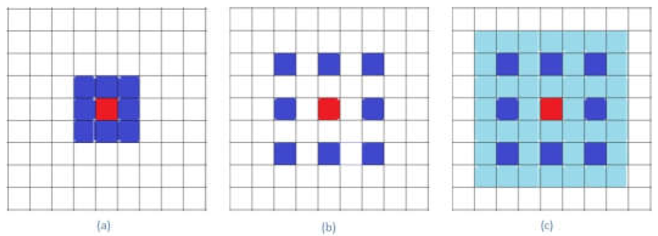
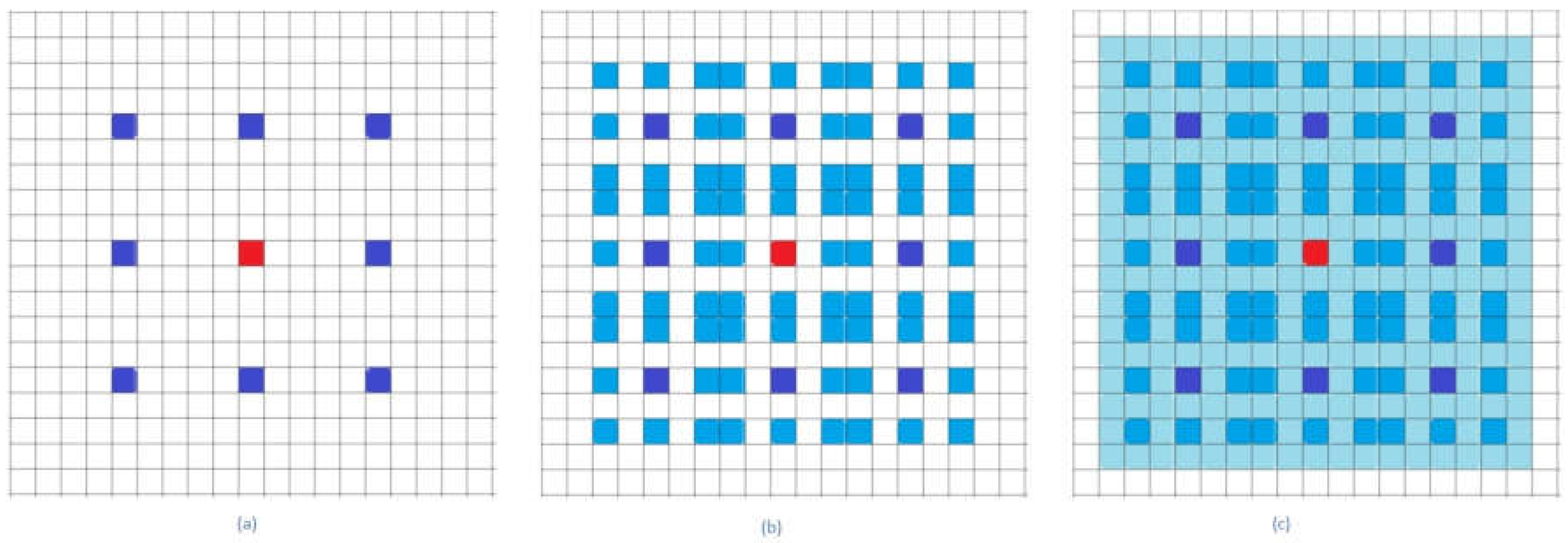
In a dense atrous convolution block, the receptive fields of each convolutional module increase significantly as the level increases. As Figure 1a shows, the receptive field of the first level atrous convolution module only covers a 3 × 3 space. In Figure 1b,c, the sampling points of the second level atrous convolution module are not continuous. However, the module receptive fields cover a 7 × 7 space after the module’s result is combined with the result of the first level module. In Figure 2, the receptive fields of the third level atrous convolution module cover a 17 × 17 spatial space. The receptive fields of a dense atrous convolution block cover a 33 × 33 spatial space. Each atrous convolution module in the dense atrous convolution block has a certain output feature-maps. This size of feature-maps is known as the block’s growth rate. The level convolution module of the dense atrous convolution block has a input feature-maps, where denotes the block’s input.
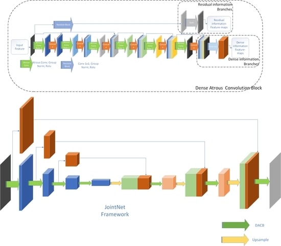
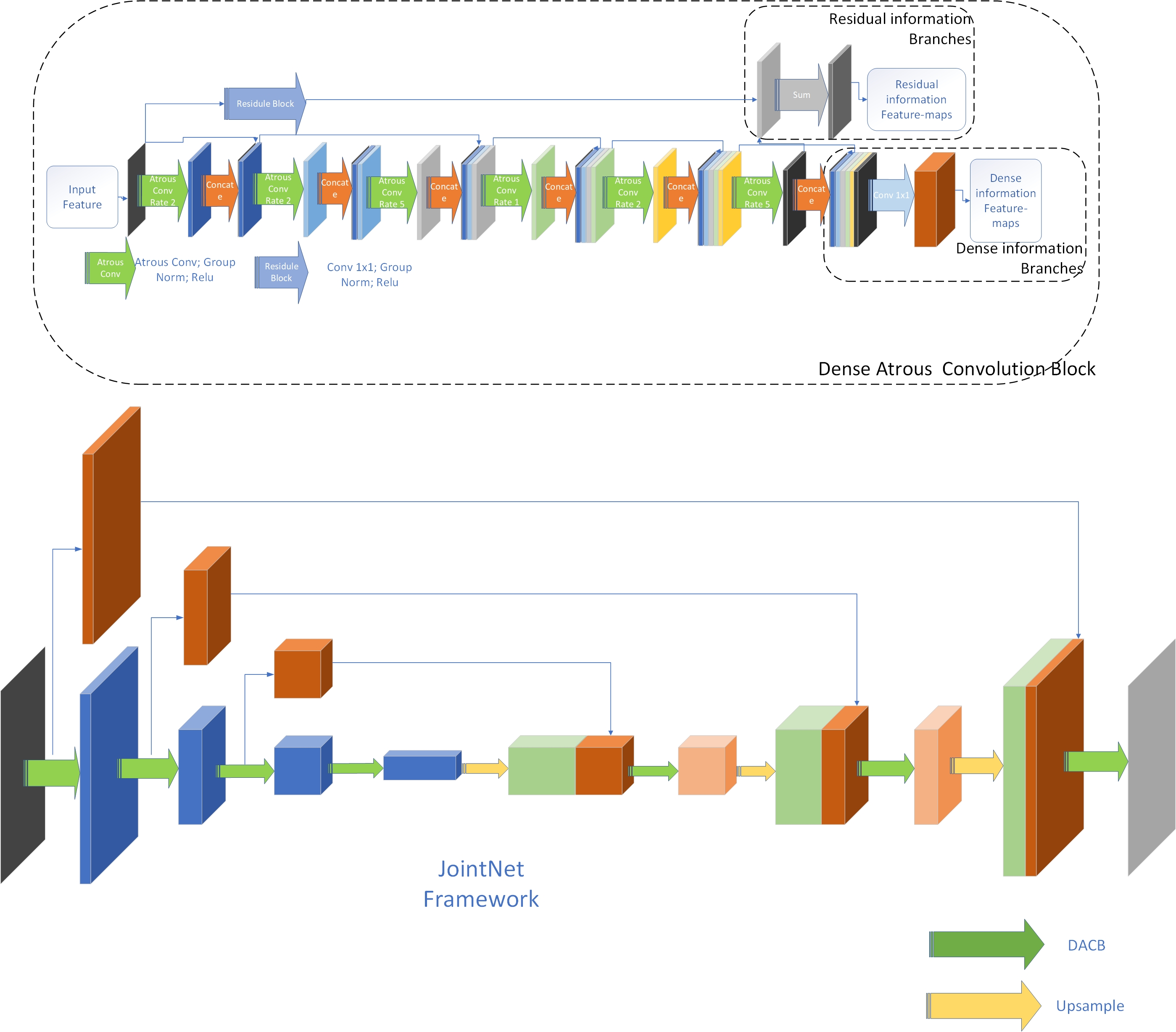
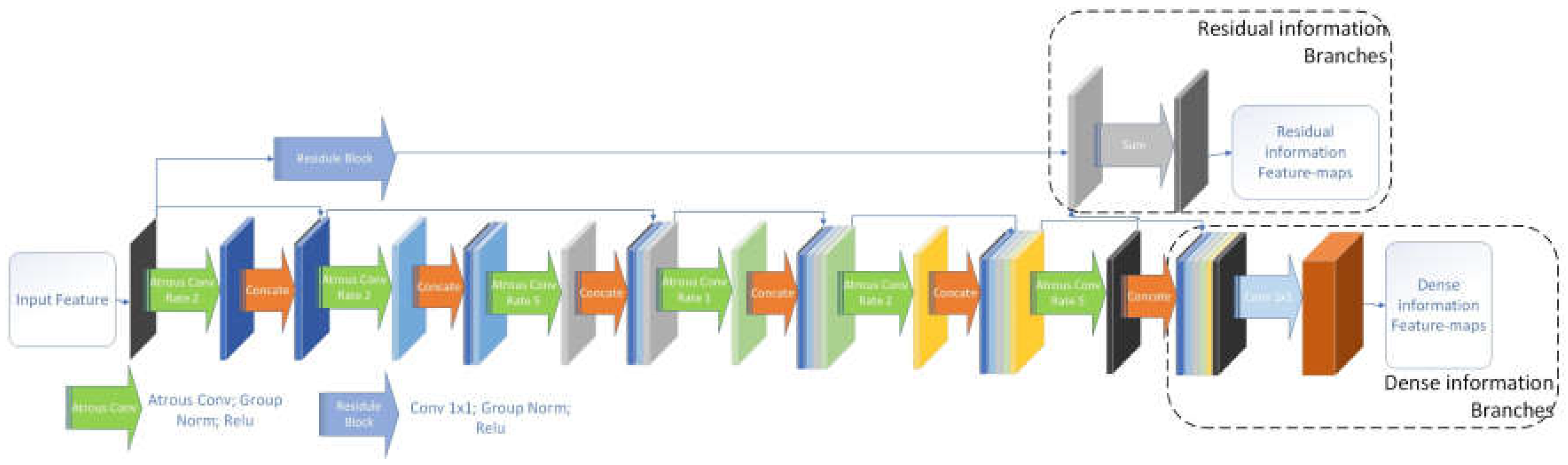
As the information loss caused by down-sampling cannot be recovered by up-sampling [40], the semantic information of high-level encoders in the encoder-decoder network cannot be fully recovered by multi-layer decoders. This shortcoming affects the extraction of some morphologically sensitive ground object information, such as the road centerline. As shown in Figure 3, to solve this problem better, our proposed module designs two information branches: one is the residual information branch for information flow between coders and decoders at different levels of encoding/decoding paths, and the other one is the dense information branch for information flow from the encoders to their corresponding level decoders with the same scale feature-maps. The residual information branch uses the module input to fuse the output feature-maps of the last layer atrous convolution as residual information output of the module. The dense information branch uses a 1 × 1 convolution layer to compress the module’s context into feature-maps. The k denotes the module growth rate. The parameters of each convolutional layer of the module are shown in Table 1.
3.2. JointNet Architecture
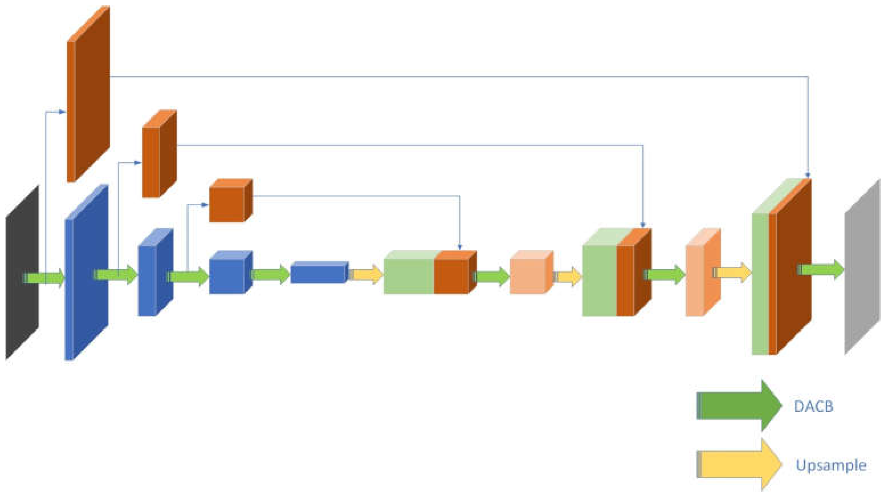
JointNet consists of an encoding path, a decoding path, a network bridge module, and a classification layer. The encoding path consists of three level upper-to-down encoders with different size feature-maps. The decoding path includes three corresponding decoders. All encoders, decoders, and network bridge modules in the network are dense atrous convolution blocks. The classification layer of the network is a convolution layer.
As Figure 4 shows, the residual information feature-maps of the encoder at each level are used as the input of the downside level encoder or network bridge module. The dense information feature-maps of the encoder is passed to the corresponding level decoder. The decoder uses the concatenation of the dense feature-maps and amplified residual feature-maps from the downside level decoder as its input feature-maps. The parameters of each module of the network are shown in Table 2.
3.3. Group Normalization and Focal loss
3.3.1. Group Normalization
Compared with the image classification networks [1,2,3,37,41], the semantics segmentation networks [6,19] cost more memory space. For this reason, the training batch size of the semantics segmentation networks is usually smaller than that of image classification networks in the same hardware environment. Since the batch size is small, the training error of the networks’ batch normalization (BN) [10] layers increase rapidly which costs poor performance of the network’s training result. Therefore, the semantic segmentation networks with BN layers need to find a balance between the smaller network model with a larger batch size and a larger model with a smaller batch size.
Group normalization (GN) [11] is a newly proposed normalization method which is barely affected by batch size. The feature allows the network to use larger models for better results which makes GN more suitable for semantic segmentation networks than other comparison normalization methods.
The BN, layer normalization (LN) [42], instance normalization (IN) [43] and GN layer share the same computation:
In Equation (3), is the feature-map in a neural network layer with the index . In the two-dimensional fully convolution network, the feature-maps of each layer is a four-dimensional vector denoted as . is the batch size. is the channel size. and are the height and width sizes of the feature-maps, respectively. The and are denoted as the running mean and standard deviation (std) of the normalization layer, respectively:
In Equation (4), the denotes the subset of feature-maps where the running mean and std are computed. In BN, this set is defined as follows:
The and the denote the sub-indexes and along the axis, respectively. In the BN layer, the running mean and std are computed in one training batch. In the case of a high memory costs neural network model, the batch size must be small. The running mean and std of the BN layer fluctuate highly, resulting in a high training error which affects the network’s training result. The GN layer overcomes the batch size problem by defining its computing set of feature-maps as below:
In Equation (6), hyper-parameter is the number of groups. is the number of channels per group. means that the indexes and are in the same group of channels. GN computes its running mean and std along these groups of channels which are not affected by batch sizes.
3.3.2. Focal Loss
The focal loss [9] is proposed to address the dense object detection issue. This loss function is more sensitive than the cross-entropy loss (CE) in the foreground-background imbalance case. We found however that the focal loss is suitable for the detection of both dense objects and linear shape objects, such as the road centerline, the outside shape of buildings and some medical images. Among these tasks, the objectives that need to be classified are extremely unbalanced. By changing the loss function, the same neural network structure can achieve significant improvement.
Cross-entropy loss (CE) is an essential method for multi-classes classification; below is the CE function for binary classification:
In Equation (7), is the estimated probability in specific class labeled with . For convenience, here we define the probability as:
There is an improved modification of CE known as balanced cross entropy loss (Balanced CE) to address the class imbalance issues. This loss function introduces a class weight factor for class and for class otherwise. In practice, this class weight factor is a non-differentiable hyperparameter which can only set by cross-validation. We use to replace and in the definition equation:
The weight factor cannot be differentiable, so the balanced CE cannot feedback the essential balance rate between the easy/hard negatives in the foreground-background imbalance condition. As such, a large number of easy negatives occupy a major part of the loss and guide the gradient. To focus the loss on the hard negatives, the focal loss function uses to replace . This factor introduces as the focusing parameter. In Equation (10), there is the equation for the focal loss (FL):
The focal loss has two properties: (1) when an example is misclassified, the loss is close to CE and the weights factor gets rare effects (, the weight factor ); when , the weights factor pulls down the weight of easily classified samples. (2) The focusing parameter is used to adjust the down-weighted rate of easy samples. When , FL is equal to CE. The down-weighted effect of easy samples is increased since gets bigger.
4. Experiment and Analysis
We verified the effectiveness of the proposed method on three datasets: Massachusetts road and building datasets [7], and National Laboratory of Pattern Recognition (NLPR) road dataset [44]. The proposed JointNet is compared with the other CNN architectures which have been verified on these datasets. This section describes the experimental datasets, data augmentation methods, compared methods, metrics, and results.
4.1. DataSets
4.1.1. Massachusetts Road and Building Datasets
Massachusetts dataset was built by Mnih et al. [7], consisting of two sub-databases, roads and buildings. It is the first publicly opened dataset for CNN training. Each image of the dataset is 1500 × 1500 pixels with spatial resolution at 1 m per pixel. The Massachusetts road datasets were generated from centerline data from the OpenStreetMap [45] project. The road line thickness was set as 7 pixels, consisting of 1108 trainings, 14 validations and 49 testing images. The Massachusetts building sub-datasets consist of 151 aerial images of the Boston area, including 137 trainings, 4 validations, and 10 testing images. The ground truth of the building dataset was transformed from building footprints of the OpenStreetMap project. This database contains buildings of all sizes, including factory floors, residences, gas stations and shopping malls.
4.1.2. National Laboratory of Pattern Recognition (NLPR) Road Datasets
NLPR road datasets were built by Cheng et al. [44], consisting of 224 images. The ground truth of these datasets includes road area segmentation and centerline. In our experiment, we evaluated the methods on the segmentation dataset. We used the 1st ~ 180th images of the dataset as the training set, the 181th ~ 194th images as the validation set, and the 195th ~ 224th images as the testing set.
4.2. Data Augmentation
In the above experimental datasets, we use some data augmentation methods to generalize the limited data. These methods have two levels of data augmentation: morphological and image transformation.
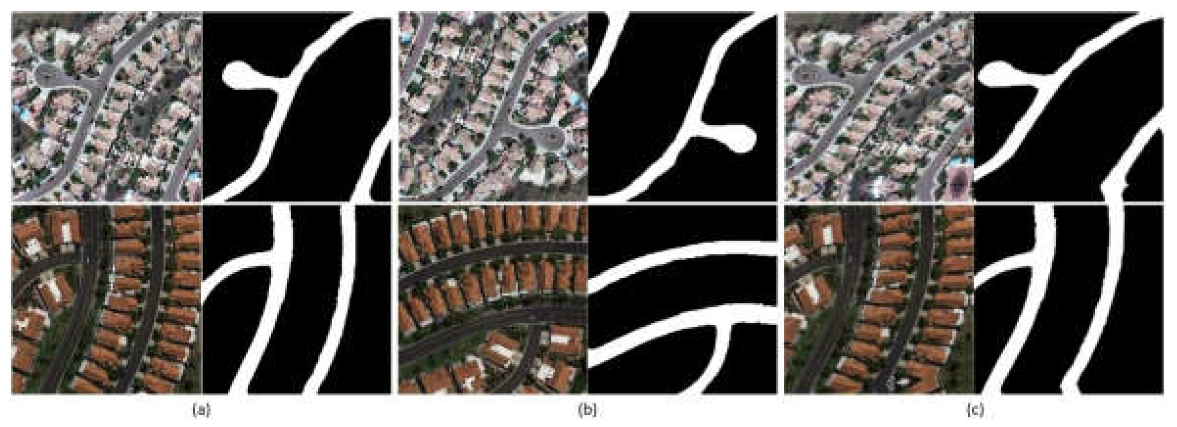
The implementation methods for morphological transformation, the first level data augmentation, are elastic deformation [46] and random flip. Both methods are synchronous morphological changes of the image and of its ground truth. Elastic deformation generates a random displacement field at first. Based on the displacement field, the method performs affine transformation synchronously on the image and its ground truth. Image random flip is a method which synchronously and randomly flips an image and its ground truth. Figure 5 shows the effect of the two data enhancement methods, elastic deformation and random flip, on the image and its ground truth.
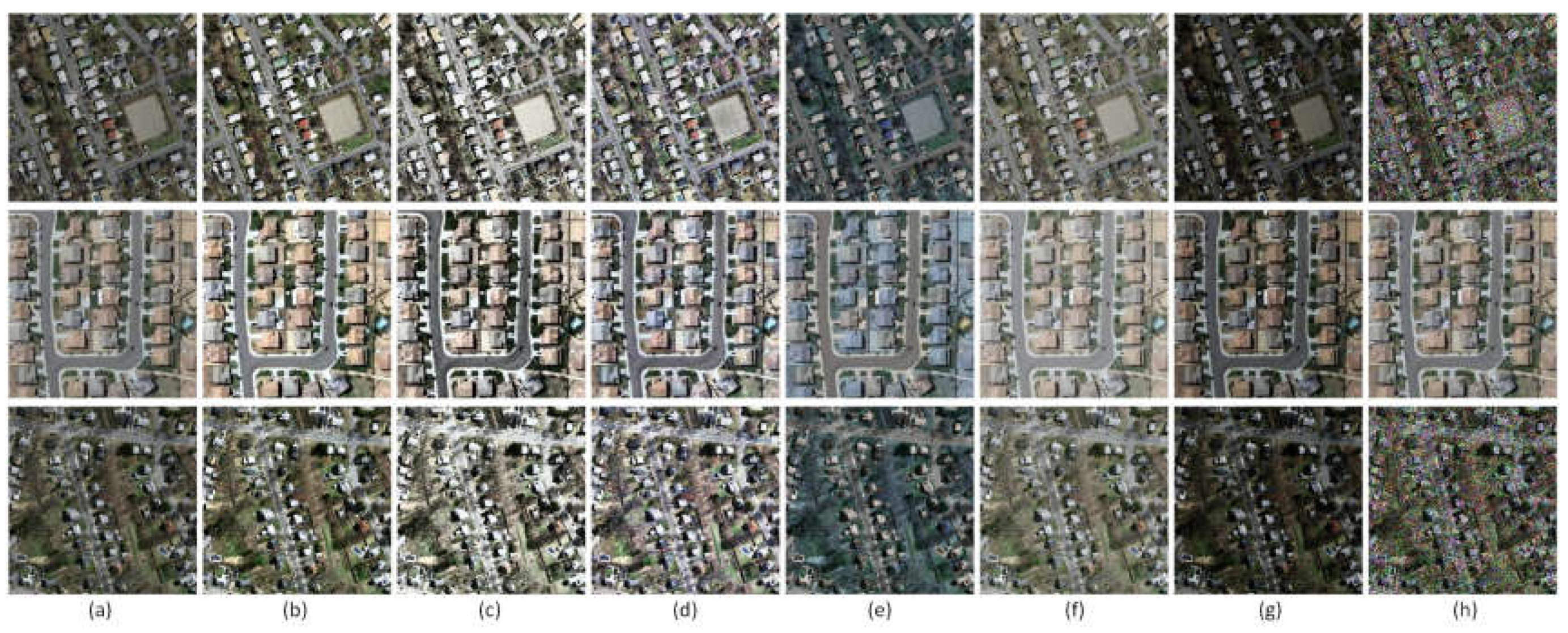
The second level of data augmentation is image transformation, which includes contrast stretching, gamma correction, histogram equalization, adaptive histogram equalization and random noise. The image transformation method does not involve morphological changes, so the image’s ground truth does not change. Contrast stretching is a linear transformation that stretches an arbitrary interval of the image intensities and fits it to another interval. Histogram equalization is a nonlinear transformation that stretches the area of the color histogram with high abundance intensities and compresses the area with low abundance intensities. Adaptive histogram equalization is an improved version of histogram equalization. The method transforms each pixel using histogram equalization from the pixel’s neighborhood region. Color Space Convert is the transformation that changes the color space of one image. Gamma correction is a nonlinear transformation that encodes and decodes luminance or tristimulus values of the image. In our practice, we used gamma = 0.7 and gamma = 1.5 to change the image’s luminance. Adding Random Noise is the image brightness or color transformation by adding a random matrix. In our practice, random noise methods include Gaussian noise, salt and pepper noise, Poisson noise and speckle noise.
Figure 6 shows the effect of the six data enhancement methods, contrast stretching, histogram equalization, adaptive histogram equalization, color space convert, gamma correction and random noise.
4.3. Baseline Methods
The method by Mnih et al. [7] is a Restricted Boltzmann Machines (RBM) framework with pre-processing and post-processing methods. The RBM framework contains 4096 input units, 4096 hidden units, and 256 output units. The input of this method is a three-channel color image sized and its corresponding center position ground truth sized . The method by Saito et al. [17] is a CNN method without the pre-processing step. It consists of three convolutional layers, one pooling layer, and two fully connection layers. The network’s input image and output ground truth are the same as those of the method by Mnih et al. The CasNet by Cheng et al. [44] contains a road detection network and a centerline extraction network. Both of them are the encoder-decoder structure CNN’s method, the state-of-the-art method on NLPR dataset. The U-Net by Ronneberger et al. [19] is an encoder-decoder structure CNN method. This network improves its performance by transmitting the feature-maps generated in the encoder to the corresponding decoder. The Res-U-Net by Zhang et al. [18] is an improved method based on U-Net. By adding a residual transfer module, this network improves the accuracy of segmentation. This method is the state-of-the-art method on the Massachusetts road dataset. The D-LinkNet by Zhou et al. [47] is the winner of the DeepGlobe 2018 [48] road challenge. The Multi-Stage Multi-Task Neural Network (MTMS) by Marcu et al. [24] is an encoder-decoder structure CNN network, the state-of-the-art method on the Massachusetts building dataset. The TernausNetV2 by Iglovikov et al. [49] is an encoder-decoder structure CNN network method.
4.4. Experimental Metrics
The experimental metrics of this work include correctness, completeness, quality, precision/recall (PR) plot and relaxed precision/recall (PR) plot. Correctness and completeness are also called as precision and recall, respectively, in computer science literature.
In the binary classification, if the positive/negative recognizable object is labeled as respectively, the range of predicted results of the training model will be . When calculating correctness, completeness, and quality, a threshold should be set in advance which is typically 0.5. The samples whose prediction value is greater than or equal to the threshold are positive, and those whose prediction value is less than the threshold are negative. According to the combination of ground truth (GT) and prediction results, all samples were divided into true positive (TP), false positive (FP), true negative (TN) and false negative (FN). Where the correctness/precision, completeness/recall are defined as follows:
It is not enough to verify the accuracy of the binary classification model only by correctness and completeness rates, because once the threshold changes, the correctness and completeness rates will change accordingly. Therefore, to further measure the effect of the classifier, we use quality, which evaluates the harmonic average of completeness and correctness in remote sensing literature.
Different from precision and recall, the precision/recall plot is not only two values but a systematical evaluation result. The plot is formed by a series of connected vertices. Each vertex is measured by setting the positive/negative thresholds to a sequence of equal difference from 0.0 to 1.0. The values of correctness and completeness correspond to a point on the plot if and only if the threshold is equal to 0.5. In the precision/recall plot measurement, if the plot of one method can completely enclose the plot of the other method, which means the former method achieve better precision/recall result in every threshold condition, it can be concluded that the performance of the former method is better than the latter. The break-even point of the plot is an important but incomplete measurement of binary classification. However, compared with the measurement based on one single threshold, the precision/recall plot shows a complete test scenario in every threshold standard.
Considering the difficulty in accurately labeling recognizing objects in large-scale remote sensing images, Mnih et al. [7] introduced the relaxed precision/recall plot [50] as a practical metric on these datasets. The relaxed precision/recall introduces a buffer range of ρ. Within the range of ρ pixels from any positively labeled pixel of the ground truth, each pixel predicted as positive is considered to be correctly classified.
4.5. Results
4.5.1. Experimental Result on the Massachusetts Road Dataset
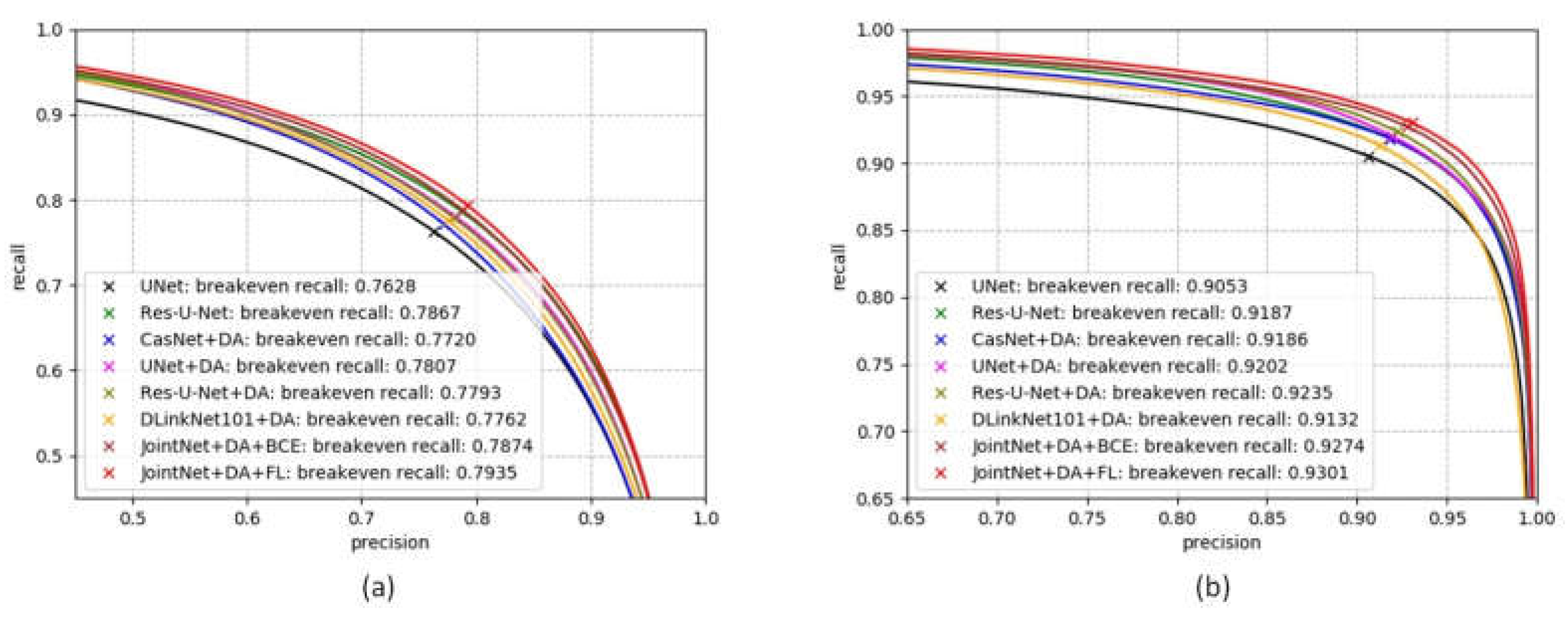
In the Massachusetts road dataset evaluation, the baseline methods include U-Net [19], Res-U-Net [18], CasNet [44], D-LinkNet [47], and early results from Mnih et al. [7] and Saito et al. [17]. In our experiment, as Figure 7 shows, the U-Net and the Res-U-Net models were implemented using Keras [51]. These two models were trained with an image block sized . The two models used Adam [52] as their optimization method with an initial learning rate at 0.0001. The loss function for these two baseline models was mean squared error (MSE). The CasNet, the U-Net+DA, the Res-U-Net+DA and the D-LinkNet+DA models were implemented using Pytorch [53] and trained with a data-augmented image block sized . The loss function for these three baseline models was binary cross-entropy (BCE). The two JointNet models were then implemented using Pytorch and trained with a data-augmented image block sized . The JointNet+DA+BCE model used the BCE as its loss function. The JointNet+DA+FL model used focal loss [9] (FL) as its loss function. All the models implemented with Pytorch used Adam [52] as their optimization method with an initial learning rate at 0.0001.
From the precision/recall plots in Figure 7 and evaluation results listed in Table 3, we can see that our proposed method, JointNet, set the new state-of-the-art on this dataset. The proposed method reached the best performance result on the break-even point of standard precision/recall plot, the break-even point of relaxed precision/recall plot and quality metrics among all the comparison methods. Note that the proposed method is a convolutional neural network method without any post-processing steps which can improve model performance. The CasNet reached the best performance on correctness and the D-LinkNet reached the best performance on completeness metrics.
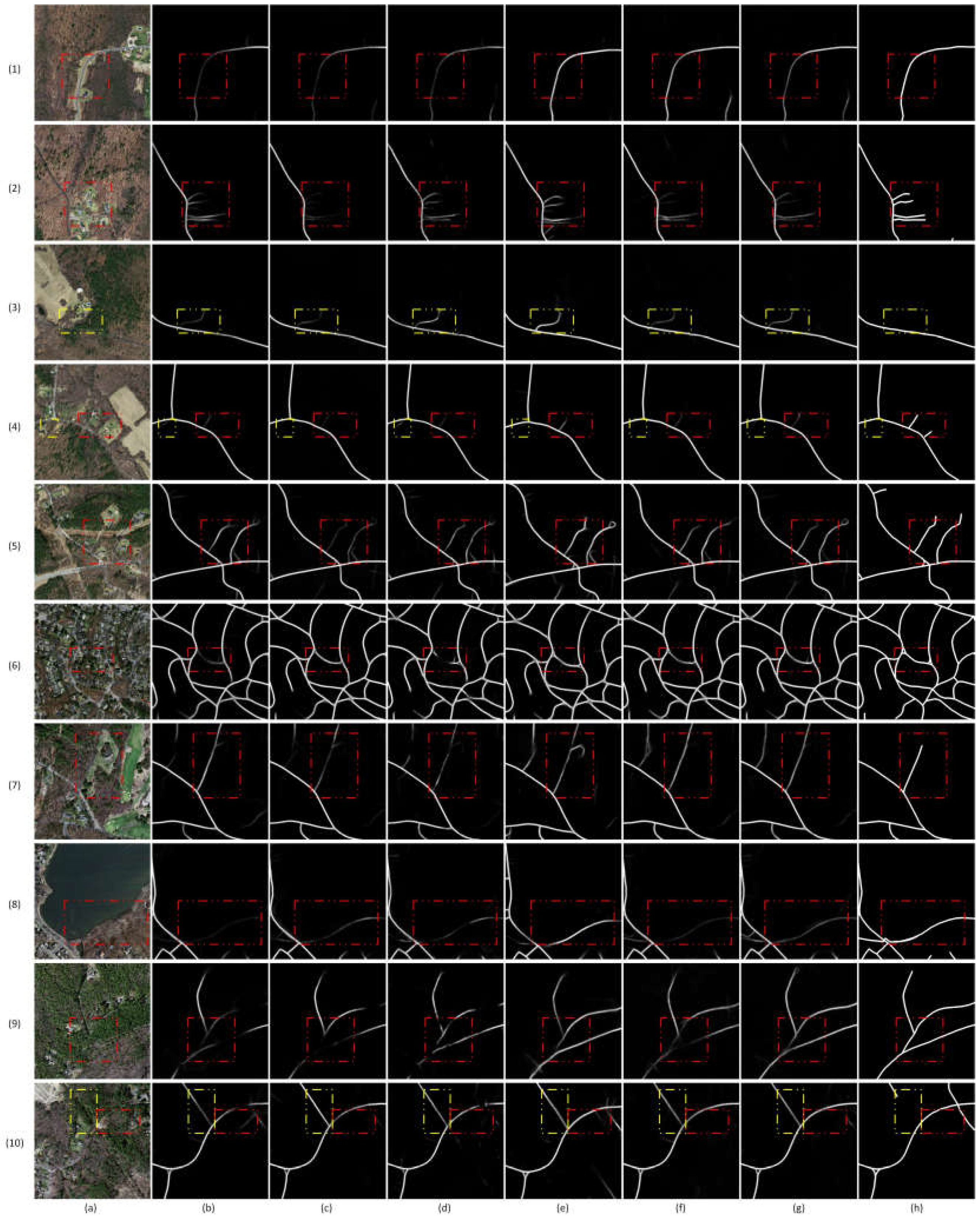
As shown in Figure 8, the image areas are labeled by red dotted frames which are correctly marked but poorly recognized road targets. Here, we call these targets the first category targets. The image areas are labeled by yellow dotted frames which contain suspicious unmarked roads in the ground truth. We call these targets the second category targets.
In the first step, we compared the differences between the results of different network models. In Figure 8, the columns b, c, d, e, and f were the testing results of CasNet, U-Net, Res-U-Net, D-linkNet101, and JointNet models, respectively. These models were trained with the same data and the binary cross-entropy loss function. CasNet performed well in some parts, such as the 2nd, 4th and 7th rows. In other places, the result’s error rate was very high, such as the 1st, 6th, 8th, 9th and 10th rows. Some identified road targets from the results of U-Net and Res-U-Net models were obviously discontinuous, such as the 7th, 8th and 9th rows. The evaluation results showed that D-linkNet101 performed best in terms of completeness rate. The method performed best among all the methods of comparison in the 1st, 3rd, 5th and 8th rows. However, the method also had obvious errors in the 7th and 10th rows. This method showed good robustness for identifying roads with insignificant features such as the 3rd and 4th rows. Through the evaluation of the precision/recall plot and the quality item, our proposed model, JointNet, performed best among all methods of comparison. The road extracted by this method has no obvious error. The continuity and consistency of the road extracted by this method are good. In the recognition of the second category targets, JointNet has no obvious advantage over the baseline methods.
In the second step, we compared the differences between the two JointNet models trained with the BCE and FL functions, respectively. In Figure 8, the columns f and g are the testing results of the two models, respectively. Comparing one model with the other on the recognition of the first category targets, the model trained with FL performed better in every row than the one trained with BCE. For the second category targets recognition, from the 3rd, 4th and 10th rows, the model trained with FL produced better results than the model trained with BCE.
The above two steps and evaluation results showed that the proposed neural network, JointNet, reached higher accuracy in the road centerline extraction task than other networks. The proposed method had the advantage in the continuity of road extraction result. The focal loss function improved road centerline extraction accuracy in our proposed method.
4.5.2. Experimental Result on the NLPR Road Dataset
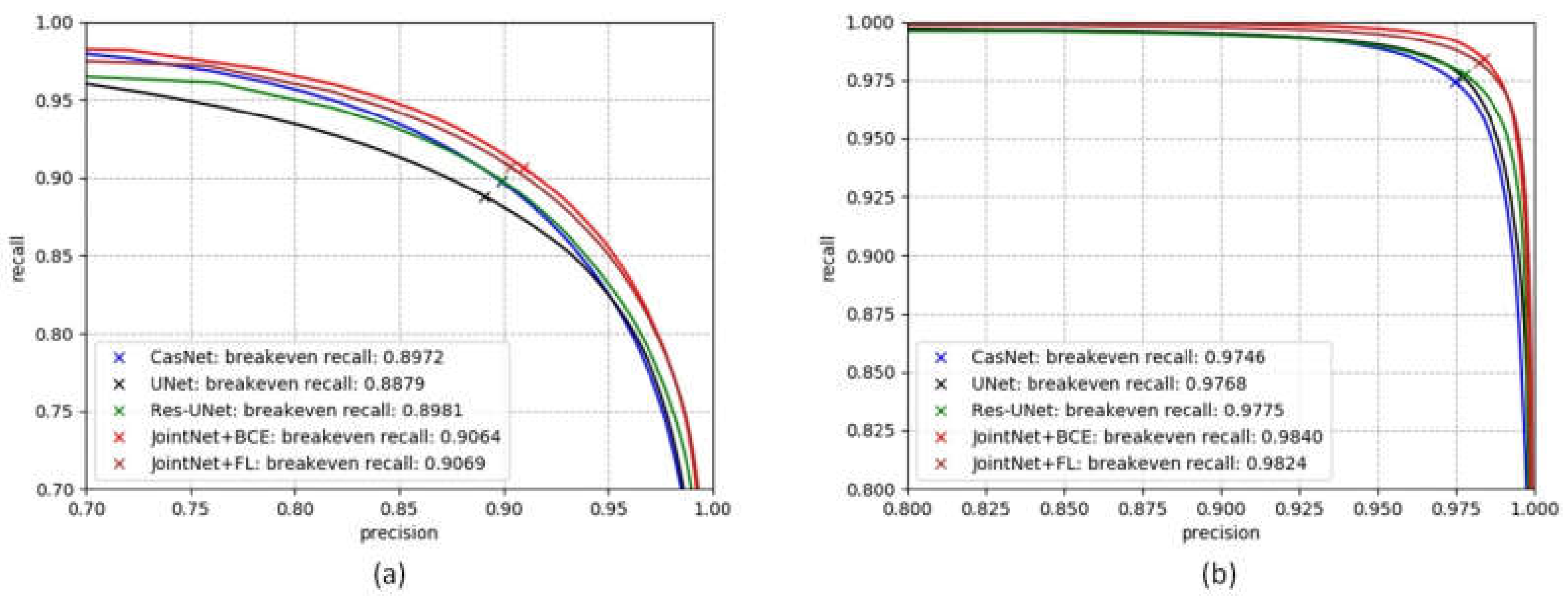
In the NLPR road dataset evaluation, the baseline methods include CasNet [44], U-Net [19], and Res-U-Net [18]. The proposed method, JointNet, and all baseline methods were implemented using Pytorch [53]. The baseline networks were trained with a data-augmented image block sized , and the loss function was binary cross-entropy (BCE). The two JointNet models were also trained with a data-augmented image block sized . The JointNet+BCE model used the BCE as loss function, and the JointNet+FL model used focal loss [9] (FL) as loss function. All the models used Adam [52] as their optimization method with an initial learning rate at 0.0001.
The precision/recall plots in Figure 9 and evaluation results listed in Table 4 show that our proposed method, JointNet, reached better performance results than the baseline methods. The proposed method produced a better result than baseline methods on all metrics, including the break-even point of standard precision/recall plot, the break-even point of relaxed precision/recall plot, correctness, completeness and quality. Between the two models of our proposed method, the model trained with focal loss performed better in the break-even point of standard precision/recall plot and correctness. The model trained with binary cross-entropy loss performs better in the break-even point of relaxed precision/recall, completeness and quality metrics.
As shown in Figure 10, the overall performance of JointNet was the best and most stable. The testing result of the proposed method reached the lowest error rate in the road area nearby trees and shadows. Note that the CasNet is the only network in comparison without the skip-connection module. This model performed unexpectedly well in the 1st, and 3rd rows, but weak in the area nearby shades, such as the 2nd, 4th and 6th rows. The Res-U-Net model has a limitation on the size of its receptive field. In the 5th row, there are forks in front of the house beside the road. The Res-U-Net model produced many errors in the environment. However, JointNet, which has a larger receptive field than the Res-U-Net model, reached a low error rate under the same condition.
The above analysis and testing results showed that the proposed neural network, JointNet, reached higher road segmentation recognition accuracy than the baseline methods. The proposed method which has larger sized receptive fields than that of the baseline methods recognized a wider range of context information and obtained more accurate results. In addition, there was no evidence that the network model trained with the focal loss function was superior to the model trained with the binary cross-entropy loss function on the road segmentation extraction task.
4.5.3. Experimental Results on Massachusetts Building Dataset
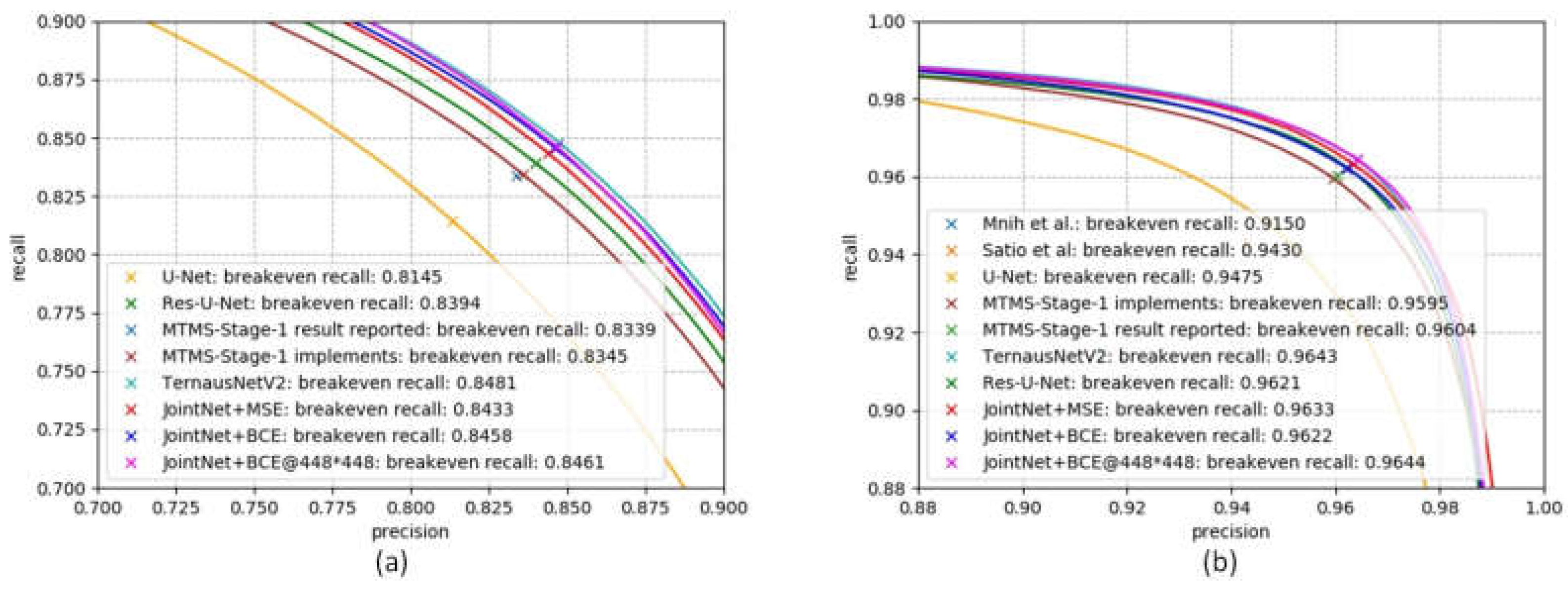
In the Massachusetts building database evaluation, the comparison methods include MTMS [24], U-Net [19], and Res-U-Net [18]. The current state-of-the-art method, the MTMS, was implemented using Keras. In order to compare the state-of-the-art method with the proposed method, all network models tested in this evaluation were implemented using Keras. The baseline network models were trained with the image block sized . The experimental results showed that there was little difference between the results of MTMS reported and our MTMS implementation. The results of our MTMS implementation were slightly better than those of MTMS reported in standard precision/recall and slightly lower in the relaxed precision/recall. To better evaluate the effectiveness of the proposed method, the TernausNetv2 by Iglovikov et al. [49] was added to the baseline methods. The method is an encoder-decoder network utilizing the pre-trained residual network to reach a better classification accuracy. Our proposed method, JointNet, used two different loss functions, mean-square error (MSE) and binary cross-entropy (BCE). Two JointNet models were trained with the image block sized . Another JointNet model was trained with the large image blocks sized using BCE as loss function. All these models used Adam [52] as their optimization method with an initial learning rate at 0.0001.
According to the precision/recall plots in Figure 11 and results listed in Table 5, the TernausNetV2 performed well on the break-even point of standard precision/recall plot, completeness and quality. Our proposed method performed well on the break-even point of relaxed precision/recall plot and correctness. Between the two models of our proposed method which were trained with image blocks sized , the model trained with BCE performed slightly better in standard precision/recall and the model trained with MSE performed better in the relaxed precision/recall. Surprisingly, the model trained with larger size image blocks () did not achieve better results than the model trained with smaller blocks.
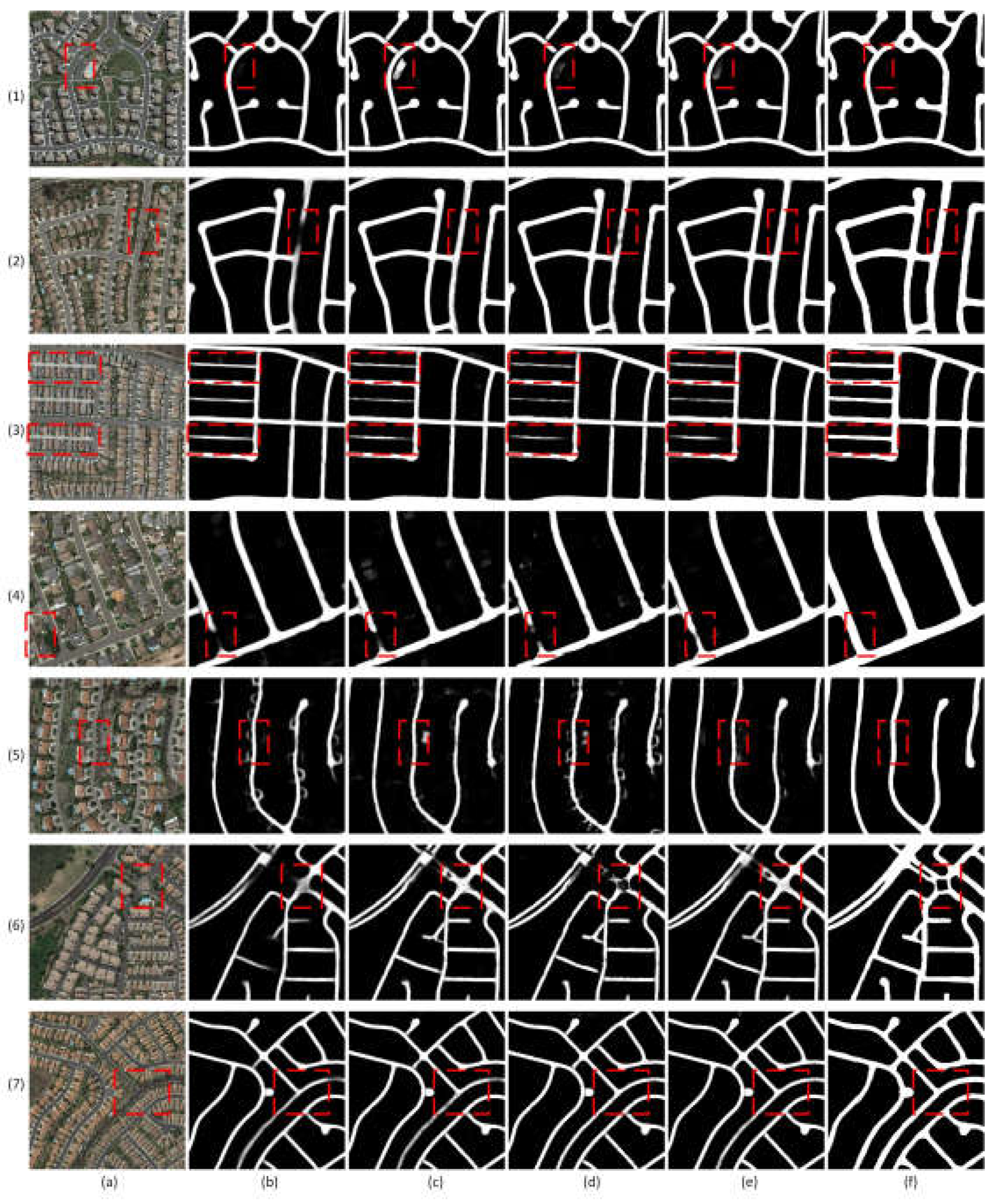
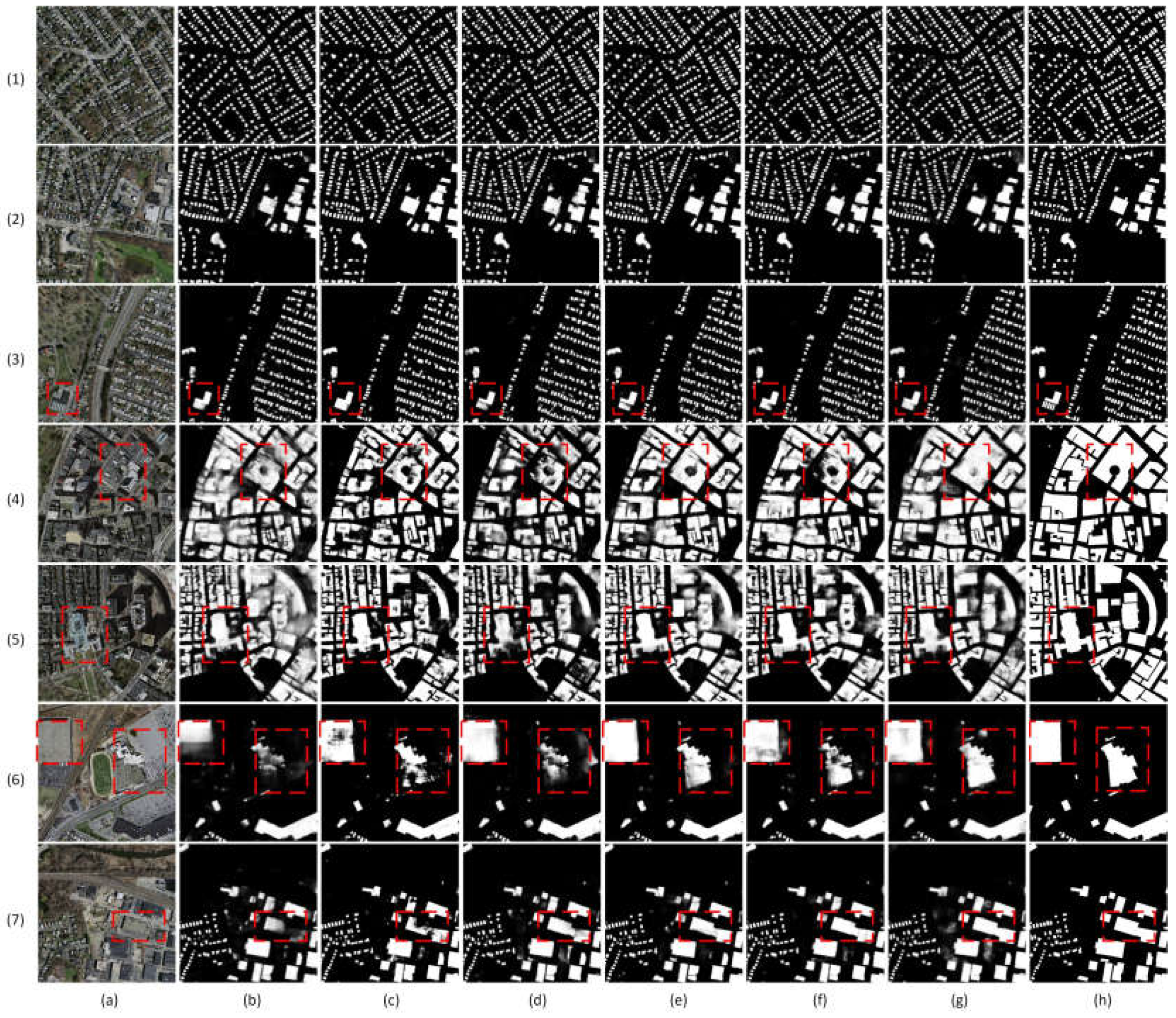
As shown in Figure 12, in the 1st, 2nd and 3rd rows, there was little difference in the extraction of small size building targets among the methods in comparison. In the 3rd row, the two models, U-Net and MTMS, had no normalization module but provided more details of building separation. From the results in the 4th, 5th, 6th and 7th rows, the size of the network’s receptive field played a very important role. In the 4th row, the building was marked with a red dotted frame whose color and texture were similar to those of road surface. The result of the Res-U-Net model showed discontinuity in the central area of the building. The main reason for the discontinuity of the center of the large building extraction results was that the receptive field of the network was too small to cover the building. The discontinuity also happened in the MTMS model’s results. The TernausNetV2 and the JointNet models achieved better recognition results than that of the MTMS. In the 5th row, the boundary of the building was clear from the image. The U-Net, the Res-U-Net, the TernausNetV2, and the JointNet models extracted better results of the building boundary than that of the MTMS. The Res-U-Net distinctly extracted the outline of all buildings in the shadow environment, while the U-Net and the TernausNetV2 performed poorly in the shadow environment. The JointNet model trained with the large size image block was also less effective than the model trained with smaller sized image blocks in building extraction in shaded environments. In the 6th row, the U-Net model did not extract large-scale buildings well. The Res-U-Net model performed well on the building boundary but poorly in the central area of the building. Due to the size of the model’s receptive fields, there was a discontinuity in the central area of the building. The TernausNetV2 model, a network that also used the residual block as its main component, had a good result because of its deeper network layers which had a larger receptive field than that of the Res-U-Net model. The MTMS model performed well on one simple shaped building and poorly on the other one which has a complex shape and texture. The JointNet and the TernausNetV2 models performed well on both large-scale buildings. The JointNet and the TernausNetV2 models were less likely to cause discontinuity in the central area of extracted large-scale buildings than the other baseline methods.
The above analysis and evaluation results revealed that the proposed method, JointNet, had the best performance on the correctness metrics. Compared with the TennausNetV2 method, the proposed method had advantages in the correctness and the break-even point of relaxed precision/recall plot. Compared with the U-Net, the Res-U-Net, and the MTMS methods, the proposed method had a larger receptive field and was less likely to cause discontinuity in the central area of extracted large-scale building targets. In addition, based on the evaluation of the proposed method, the binary cross-entropy loss function had no obvious advantage over mean-square error function on the building extraction task and the model trained with the larger size image blocks had limited improvement compared with the one trained with smaller size image blocks in the building extraction task.
5. Discussion
Buildings and roads are two kinds of objects which differ greatly in morphology, but these two kinds of objects are also the two most important man-made objects in remote sensing images of built-up areas. Many specific applications are based on information about them. Therefore, a common method that can effectively extract information from two kinds of objects has good practical value. Before convolutional neural networks were widely used in remote sensing, OBIA-based methods could not effectively extract these two types of objects in a unified framework. Mnih et al. [7] proposed the first RBM-based method for both building and road objects extraction. Since then, Saito et al. [17] and Alshehhl et al. [55] have proposed CNN-based methods that can be applied to the two kinds of ground objects.
As these two kinds of objects have their own characteristics, there are different requirements for the network which can effectively recognize these two types of ground objects.
- (1)
- In the road extraction task, the ground truth of road is a linear shape target. As the width of the target is very limited, only a few pixels, if the prediction results differ from the target location, even if by only a few pixels, the evaluation results can show a big difference. Therefore, the extraction accuracy of such targets depends on the consistency of the shape and position of the prediction results with the target. In the high-level features of convolutional networks, the spatial location information of the target becomes unstable after several rescale operations. At this time, the reuse of the low-level features becomes key, because the low-level features have not been rescaled, the spatial location information in the low-level feature is more accurate than that of the high-level feature. For this reason, the encoder-decoder network, which reuses the low-level feature by skip connection, played an important role in the road extraction task.
- (2)
- In the building extraction, the key to the building extraction network is to have a large receptive field. Accurate building extraction depends on the acquisition of the complete edge information of the building, which is distributed in a certain range in remote sensing images. A network with a large receptive field which covers the range can extract the context information of the building such as its edge. As shown in the evaluation results, if the size of the receptive field of the network is too small to cover the building target, one of the typical problems caused by this issue would be the discontinuity in the central area of the extracted large-size building target. The semantic information of the high-level features of the network covers a wider range of receptive fields than that of the low-level features, so for building extraction, the high-level features of the network are more critical than that of the low-level features.
The neural network which can be a common method for both road and building extraction must satisfy the requirements of these two kind targets at the same time. Based on the requirement of effective road extraction, the network framework needs to be in the encoder-decoder mode. Based on the encoder-decoder network, there are several ways which can effectively increase the receptive field of the network. First, by effectively organizing the atrous convolution layers, the receptive field can be enlarged within certain network depth. This method is just like the network proposed in this paper. Second, using the high-level features of the deep network to achieve a wide range of receptive fields, and collecting the low-level features of the network as the reusable information for road extraction task. A typical example of such structure networks is the TernausNetV2 [49]. Third, using pyramid pooling module (PPM), atrous spatial pyramid pooling module (ASPP), or other methods to achieve a large size receptive field.
6. Conclusions
In this paper, we propose a neural network module based on the combination of dense connectivity and atrous convolution, which fully utilizes the information flow efficiency of the dense connectivity pattern and the large receptive field of atrous convolution layer. By carefully designing the atrous convolution rate settings, the module’s receptive field uniformly covers a large area without any loopholes. Based on this module, we propose an encoder-decoder network, which can meet the performance requirements for extracting road and building information.
The evaluation results of experiments showed that the proposed method achieved higher accuracy on a road centerline extraction dataset and a road segmentation extraction dataset. The proposed method also reached high correctness on a building extraction dataset. The ground truth of these three different datasets diversifies greatly. For the ground objects of different categories, our proposed method satisfies the requirements by only changing the essential loss function. The large size receptive field of the proposed method shows different advantages in different extraction ground objects: for the extraction of the road centerline, JointNet has the advantage in the continuity of the road extraction result over the baseline methods; for the road segmentation extraction task, JointNet can recognize a larger range of the context information than that of the baseline methods and obtains more accurate results; for the building extraction tasks, the proposed method which has larger sized receptive fields was less likely to cause discontinuity in the central area of extracted large-scale building targets than the baseline methods.
It is worth noting that the training epochs of our model are rather small since our training machine only has a single graphics card at the home level. In spite of this drawback, our proposed method has achieved favorable results. It is thus believed that the model proposed will be much better after a long training time with much stronger machines.
Author Contributions
Z.Z. is a Ph.D. student at Beihang University supervised by Y.W. Y.W. gave the original idea of the article. Z.Z. designed the method, made the experiments and wrote major of the article. All authors contributed to editing and reviewing the manuscript.
Funding
This research was funded by the Foundation for Innovative Research Groups through the National Natural Science Foundation of China under Grant 61421003.
Conflicts of Interest
The authors declare no conflict of interest.
References
- Krizhevsky, A.; Sutskever, I.; Hinton, G.E. Imagenet classification with deep convolutional neural networks. In Advances in Neural Information Processing Systems; Curran Associates, Inc.: New York, NY, USA, 2012; pp. 1097–1105. [Google Scholar]
- Simonyan, K.; Zisserman, A. Very Deep Convolutional Networks for Large-Scale Image Recognition. In Proceedings of the International Conference on Learning Representations, San Diego, CA, USA, 7–9 May 2015. [Google Scholar]
- He, K.; Zhang, X.; Ren, S.; Sun, J. Deep residual learning for image recognition. In Proceedings of the IEEE Conference on Computer Vision and Pattern Recognition, Las Vegas, NV, USA, 27–30 June 2016; pp. 770–778. [Google Scholar]
- Huang, G.; Liu, Z.; Van Der Maaten, L.; Weinberger, K.Q. Densely connected convolutional networks. In Proceedings of the Computer Vision and Pattern Recognition (CVPR), Honolulu, HI, USA, 21–26 July 2017; pp. 4700–4708. [Google Scholar]
- Chen, L.C.; Papandreou, G.; Schroff, F.; Adam, H. Rethinking atrous convolution for semantic image segmentation. arXiv, 2017; arXiv:1706.05587. [Google Scholar]
- Chen, L.C.; Zhu, Y.; Papandreou, G.; Schroff, F.; Adam, H. Encoder-decoder with atrous separable convolution for semantic image segmentation. arXiv, 2018; arXiv:1802.02611. [Google Scholar]
- Mnih, V. Machine Learning for Aerial Image Labeling. Ph.D. Thesis, University of Toronto, Toronto, ON, Canada, 2013. [Google Scholar]
- Marcu, A.; Leordeanu, M. Dual local-global contextual pathways for recognition in aerial imagery. arXiv, 2016; arXiv:1605.05462. [Google Scholar]
- Lin, T.Y.; Goyal, P.; Girshick, R.; He, K.; Dollar, P. Focal Loss for Dense Object Detection. IEEE Trans. Pattern Anal. Mach. Intell. 2017, PP, 2999–3007. [Google Scholar]
- Ioffe, S.; Szegedy, C. Batch Normalization: Accelerating Deep Network Training by Reducing Internal Covariate Shift. In Proceedings of the International Conference on Machine Learning, Lille, France, 6–11 July 2015; pp. 448–456. [Google Scholar]
- Wu, Y.; He, K. Group Normalization. arXiv, 2018; arXiv:1803.08494. [Google Scholar]
- Salakhutdinov, R.; Mnih, A.; Hinton, G. Restricted Boltzmann machines for collaborative filtering. In Proceedings of the 24th International Conference on Machine Learning, Corvalis, OR, USA, 20–24 June 2007; pp. 791–798. [Google Scholar]
- Nair, V.; Hinton, G.E. Rectified linear units improve restricted boltzmann machines. In Proceedings of the 27th International Conference on Machine Learning (ICML-10), Haifa, Israel, 21–24 June 2010; pp. 807–814. [Google Scholar]
- Mnih, V.; Larochelle, H.; Hinton, G.E. Conditional restricted boltzmann machines for structured output prediction. arXiv, 2012; arXiv:1202.3748. [Google Scholar]
- Mnih, V.; Hinton, G.E. Learning to detect roads in high-resolution aerial images. In European Conference on Computer Vision; Springer: New York, NY, USA, 2010; pp. 210–223. [Google Scholar]
- Saito, S.; Aoki, Y. Building and road detection from large aerial imagery. In Proceedings of the Image Processing: Machine Vision Applications VIII, San Francisco, CA, USA, 8–12 February 2015; Volume 9405, p. 94050K. [Google Scholar]
- Saito, S.; Yamashita, Y.; Aoki, Y. Multiple Object Extraction from Aerial Imagery with Convolutional Neural Networks. Electron. Imaging 2016, 60, 10402–10402:9. [Google Scholar]
- Zhang, Z.; Liu, Q.; Wang, Y. Road extraction by deep residual u-net. IEEE Geosci. Remote Sens. Lett. 2018, 15, 749–753. [Google Scholar] [CrossRef]
- Ronneberger, O.; Fischer, P.; Brox, T. U-Net: Convolutional Networks for Biomedical Image Segmentation. In Proceedings of the International Conference on Medical Image Computing & Computer-Assisted Intervention, Munich, Germany, 5–9 October 2015. [Google Scholar]
- Blaschke, T. Object based image analysis for remote sensing. ISPRS J. Photogramm. Remote Sens. 2010, 65, 2–16. [Google Scholar] [CrossRef]
- Drăguţ, L.; Blaschke, T. Automated classification of landform elements using object-based image analysis. Geomorphology 2006, 81, 330–344. [Google Scholar] [CrossRef]
- Myint, S.W.; Gober, P.; Brazel, A.; Grossman-Clarke, S.; Weng, Q. Per-pixel vs. object-based classification of urban land cover extraction using high spatial resolution imagery. Remote Sens. Environ. 2011, 115, 1145–1161. [Google Scholar] [CrossRef]
- Maggiori, E.; Tarabalka, Y.; Charpiat, G.; Alliez, P. Fully convolutional neural networks for remote sensing image classification. In Proceedings of the 2016 IEEE International Geoscience and Remote Sensing Symposium (IGARSS, Beijing, China, 10–15 July 2016; pp. 5071–5074. [Google Scholar]
- Marcu, A.; Costea, D.; Slusanschi, E.; Leordeanu, M. A Multi-Stage Multi-Task Neural Network for Aerial Scene Interpretation and Geolocalization. arXiv, 2018; arXiv:1804.01322. [Google Scholar]
- Vincent, L.; Soille, P. Watersheds in Digital Spaces: An Efficient Algorithm Based on Immersion Simulations. IEEE Trans. Pattern Anal. Mach. Intell. 1991, 13, 583–598. [Google Scholar] [CrossRef]
- Achanta, R.; Shaji, A.; Smith, K.; Lucchi, A.; Fua, P.; SuSstrunk, S. SLIC Superpixels Compared to State-of-the-Art Superpixel Methods. IEEE Trans. Pattern Anal. Mach. Intell. 2012, 34, 2274–2282. [Google Scholar] [CrossRef] [PubMed]
- Long, J.; Shelhamer, E.; Darrell, T. Fully convolutional networks for semantic segmentation. In Proceedings of the IEEE Conference on Computer Vision and Pattern Recognition (CVPR), Boston, MA, USA, 8–12 June 2015; pp. 3431–3440. [Google Scholar]
- Eigen, D.; Fergus, R. Predicting depth, surface normals and semantic labels with a common multi-scale convolutional architecture. In Proceedings of the IEEE International Conference on Computer Vision, Santiago, Chile, 7–13 December 2015; pp. 2650–2658. [Google Scholar]
- Pinheiro, P.H.; Collobert, R. Recurrent convolutional neural networks for scene labeling. In Proceedings of the 31st International Conference on Machine Learning (ICML), Beijing, China, 21–26 June 2014; pp. 82–90. [Google Scholar]
- Lin, G.; Shen, C.; Van Den Hengel, A.; Reid, I. Efficient piecewise training of deep structured models for semantic segmentation. In Proceedings of the IEEE Conference on Computer Vision and Pattern Recognition (CVPR), Las Vegas, NV, USA, 27–30 June 2016; pp. 3194–3203. [Google Scholar]
- Chen, L.C.; Yang, Y.; Wang, J.; Xu, W.; Yuille, A.L. Attention to scale: Scale-aware semantic image segmentation. In Proceedings of the IEEE Conference on Computer Vision and Pattern Recognition (CVPR), Las Vegas, NV, USA, 27–30 June 2016; pp. 3640–3649. [Google Scholar]
- Badrinarayanan, V.; Kendall, A.; Cipolla, R. Segnet: A deep convolutional encoder-decoder architecture for image segmentation. arXiv, 2015; arXiv:1511.00561. [Google Scholar] [CrossRef] [PubMed]
- Chen, L.C.; Papandreou, G.; Kokkinos, I.; Murphy, K.; Yuille, A.L. Deeplab: Semantic image segmentation with deep convolutional nets, atrous convolution, and fully connected crfs. IEEE Trans. Pattern Anal. Mach. Intell. 2018, 40, 834–848. [Google Scholar] [CrossRef] [PubMed]
- Zhao, H.; Shi, J.; Qi, X.; Wang, X.; Jia, J. Pyramid Scene Parsing Network. In Proceedings of the Computer Vision and Pattern Recognition (CVPR), Honolulu, HI, USA, 21–26 July 2017; pp. 6230–6239. [Google Scholar]
- He, K.; Zhang, X.; Ren, S.; Sun, J. Identity mappings in deep residual networks. In European Conference on Computer Vision; Springer: New York, NY, USA, 2016; pp. 630–645. [Google Scholar]
- Szegedy, C.; Liu, W.; Jia, Y.; Sermanet, P.; Reed, S.; Anguelov, D.; Erhan, D.; Vanhoucke, V.; Rabinovich, A. Going deeper with convolutions. In Proceedings of the IEEE Conference on Computer Vision and Pattern Recognition (CVPR), Boston, MA, USA, 8–12 June 2015; pp. 1–9. [Google Scholar]
- Szegedy, C.; Vanhoucke, V.; Ioffe, S.; Shlens, J.; Wojna, Z. Rethinking the inception architecture for computer vision. In Proceedings of the IEEE Conference on Computer Vision and Pattern Recognition (CVPR), Las Vegas, NV, USA, 27–30 June 2016; pp. 2818–2826. [Google Scholar]
- Szegedy, C.; Ioffe, S.; Vanhoucke, V.; Alemi, A.A. Inception-v4, inception-resnet and the impact of residual connections on learning. In Proceedings of the 31st AAAI Conference on Artificial Intelligence, San Francisco, CA, USA, 4–9 February 2017; pp. 4278–4284. [Google Scholar]
- Wang, P.; Chen, P.; Yuan, Y.; Liu, D.; Huang, Z.; Hou, X.; Cottrell, G. Understanding convolution for semantic segmentation. In Proceedings of the 2018 IEEE Winter Conference on Applications of Computer Vision (WACV), Lake Tahoe, NV, USA, 12–15 March 2018; pp. 1451–1460. [Google Scholar]
- Frajka, T.; Zeger, K. Downsampling dependent upsampling of images. Signal Process. Image Commun. 2004, 19, 257–265. [Google Scholar] [CrossRef]
- Chollet, F. Xception: Deep Learning with Depthwise Separable Convolutions. In Proceedings of the Computer Vision and Pattern Recognition, Honolulu, HI, USA, 21–26 July 2017; pp. 1800–1807. [Google Scholar]
- Ba, J.L.; Kiros, J.R.; Hinton, G.E. Layer Normalization. arXiv, 2016; arXiv:1607.06450. [Google Scholar]
- Ulyanov, D.; Vedaldi, A.; Lempitsky, V. Instance Normalization: The Missing Ingredient for Fast Stylization. arXiv, 2016; arXiv:1607.08022. [Google Scholar]
- Cheng, G.; Ying, W.; Xu, S.; Wang, H.; Xiang, S.; Pan, C. Automatic Road Detection and Centerline Extraction via Cascaded End-to-End Convolutional Neural Network. IEEE Trans. Geosci. Remote Sens. 2017, 55, 3322–3337. [Google Scholar] [CrossRef]
- OpenStreetMap Contributors. OpenStreetMap. Available online: https://www.openstreetmap.org (accessed on 20 March 2019).
- Simard, P.; Steinkraus, D.; Platt, J.C. Best Practices for Convolutional Neural Networks Applied to Visual Document Analysis. In Proceedings of the International Conference on Document Analysis Recognition, Edinburgh, UK, 3–6 August 2003. [Google Scholar]
- Zhou, L.; Zhang, C.; Wu, M. D-linknet: Linknet with pretrained encoder and dilated convolution for high resolution satellite imagery road extraction. In Proceedings of the 2018 IEEE/CVF Conference on Computer Vision and Pattern Recognition Workshops (CVPRW), Salt Lake City, UT, USA, 8–22 June 2018. [Google Scholar]
- Demir, I.; Koperski, K.; Lindenbaum, D.; Pang, G.; Huang, J.; Basu, S.; Hughes, F.; Tuia, D.; Raska, R. Deepglobe 2018: A challenge to parse the earth through satellite images. In Proceedings of the 2018 IEEE/CVF Conference on Computer Vision and Pattern Recognition Workshops (CVPRW), Salt Lake City, UT, USA, 8–22 June 2018. [Google Scholar]
- Iglovikov, V.I.; Seferbekov, S.; Buslaev, A.V.; Shvets, A. TernausNetV2: Fully Convolutional Network for Instance Segmentation. In Proceedings of the 2018 IEEE/CVF Conference on Computer Vision and Pattern Recognition Workshops (CVPRW), Salt Lake City, UT, USA, 8–22 June 2018. [Google Scholar]
- Ehrig, M.; Euzenat, J. Relaxed precision and recall for ontology matching. In Proceedings of the K-Cap 2005 Workshop on Integrating Ontology, Banff, AB, Canada, 2 October 2005. [Google Scholar]
- Chollet, F. Keras. Available online: https://keras.io (accessed on 20 March 2019).
- Kingma, D.P.; Ba, J. Adam: A method for stochastic optimization. arXiv, 2014; arXiv:1412.6980. [Google Scholar]
- Paszke, A.; Gross, S.; Chintala, S.; Chanan, G.; Yang, E.; DeVito, Z.; Lin, Z.; Desmaison, A.; Antiga, L.; Lerer, A. Automatic differentiation in PyTorch. NIPS-W. In Proceedings of the 31st Conference on Neural Information Processing Systems (NIPS 2017), Long Beach, CA, USA, 4–9 December 2017. [Google Scholar]
- Hamaguchi, R.; Fujita, A.; Nemoto, K.; Imaizumi, T.; Hikosaka, S. Effective Use of Dilated Convolutions for Segmenting Small Object Instances in Remote Sensing Imagery. arXiv, 2017; arXiv:1709.00179. [Google Scholar]
- Alshehhi, R.; Marpu, P.R.; Wei, L.W.; Mura, M.D. Simultaneous extraction of roads and buildings in remote sensing imagery with convolutional neural networks. ISPRS J. Photogramm. Remote Sens. 2017, 130, 139–149. [Google Scholar] [CrossRef]
Figure 1.
The receptive field of the first two level modules of the atrous convolution group: (a) Receptive field of the first level of the group, a 3 × 3 kernel atrous convolution function module rated 1. (b) Receptive fields of the second level of the group, a 3 × 3 kernel atrous convolution module rated 2. (c) Receptive field of the first and second level modules combined.

Figure 2.
The receptive field of the last level of the atrous convolution group: (a) Receptive fields of the last level of the group, the atrous convolution module rated 5. (b) Receptive fields of the group’s last two level atrous convolution modules rated 2 and 5. (c) Receptive field of the group’s first, second and third level modules combined.

Figure 3.
Dense atrous convolution blocks for JointNet.

Figure 4.
JointNet: a general neural network for road and building extraction.

Figure 5.
Morphological change methods of data augmentation: (a) Original image and its ground truth. (b) Image and its ground truth after the random flip process. (c) Image and its ground truth after the elastic deformations process.
Figure 5.
Morphological change methods of data augmentation: (a) Original image and its ground truth. (b) Image and its ground truth after the random flip process. (c) Image and its ground truth after the elastic deformations process.

Figure 6.
Image transformation methods of data augmentation: (a) Original image. (b) Image after contrast stretching. (c) Image after histogram equalization. (d) Image after adaptive histogram equalization. (e) Image after color space change. (f) Image after gamma correction (gamma = 0.7). (g) Image after gamma correction (gamma = 1.5). (h) Image after added random noise.

Figure 7.
Precision/recall plots of convolution neural networks (CNNs) performance on Massachusetts road datasets: (a) The standard precision/recall plots. (b) The relaxed (ρ = 3) precision/recall plots.
Figure 7.
Precision/recall plots of convolution neural networks (CNNs) performance on Massachusetts road datasets: (a) The standard precision/recall plots. (b) The relaxed (ρ = 3) precision/recall plots.

Figure 8.
Comparison of road extraction results on Massachusetts road datasets: (a) Input Image. (b) Result from CasNet. (c) Result from U-Net. (d) Result from Res-U-Net. (e) Result from D-linkNet101. (f) Result from JointNet+Binary Cross-entropy (BCE). (g) Result from JointNet+Focal Loss (FC). (h) Ground truth.

Figure 9.
Precision/recall plots of CNNs performance on National Laboratory of Pattern Recognition (NLPR) road datasets: (a) The standard precision/recall plots. (b) The relaxed (ρ = 3) precision/recall plots.
Figure 9.
Precision/recall plots of CNNs performance on National Laboratory of Pattern Recognition (NLPR) road datasets: (a) The standard precision/recall plots. (b) The relaxed (ρ = 3) precision/recall plots.

Figure 10.
Comparison of road extraction results on NLPR road datasets: (a) Input Image. (b) Result from CasNet. (c) Result from U-Net. (d) Result from Res-U-Net. (e) Result from JointNet. (f) Ground truth.
Figure 10.
Comparison of road extraction results on NLPR road datasets: (a) Input Image. (b) Result from CasNet. (c) Result from U-Net. (d) Result from Res-U-Net. (e) Result from JointNet. (f) Ground truth.

Figure 11.
Precision/recall plots of CNNs performance on Massachusetts building datasets: (a) The standard precision/recall plots. (b) The relaxed (ρ = 3) precision/recall plots.
Figure 11.
Precision/recall plots of CNNs performance on Massachusetts building datasets: (a) The standard precision/recall plots. (b) The relaxed (ρ = 3) precision/recall plots.

Figure 12.
Comparison of building extraction results on Massachusetts building datasets: (a) Input Image. (b) Result from U-Net. (c) Result from Res-U-Net. (d) Result from MSMT. (e) Result from TernausNetV2. (f) Result from JointNet+BCE. (g) Result from JointNet@448 × 448+BCE. (h) Ground truth.
Figure 12.
Comparison of building extraction results on Massachusetts building datasets: (a) Input Image. (b) Result from U-Net. (c) Result from Res-U-Net. (d) Result from MSMT. (e) Result from TernausNetV2. (f) Result from JointNet+BCE. (g) Result from JointNet@448 × 448+BCE. (h) Ground truth.


Table 1.
Dense atrous convolution block structure.
| Layers | Input | Kernel Size | Growth Rate | Atrous Conv Rate | Output |
|---|---|---|---|---|---|
| Atrous Conv 1 | α | 3 × 3 | k | 1 | k |
| Atrous Conv 2 | α + k | 3 × 3 | k | 2 | k |
| Atrous Conv 3 | α + 2k | 3 × 3 | k | 5 | k |
| Atrous Conv 4 | α + 3k | 3 × 3 | k | 1 | k |
| Atrous Conv 5 | α + 4k | 3 × 3 | k | 2 | k |
| Atrous Conv 6 | α + 5k | 3 × 3 | k | 5 | k |
| Conv RB(1) | α | 1 × 1 | None | 1 | k |
| Conv RB(2) | α + 6k | 1 × 1 | None | 1 | 4k |
(1) RB: Residual Information Branch. (2) DB: Dense Information Branch.
Table 2.
JointNet Architecture.
| Name | Module Type | Spatial Size | Input | Stride | GR(1) | RO(2) | DO(3) |
|---|---|---|---|---|---|---|---|
| Encoder Level 1 | DACB(4) | 3 | 1 | 32 | 32 | 128 | |
| Encoder Level 2 | DACB | 32 | 2 | 64 | 64 | 256 | |
| Encoder Level 3 | DACB | 64 | 2 | 128 | 128 | 512 | |
| Network Bridge | DACB | 128 | 2 | 256 | 256 | None | |
| Decoder Level 3 | DACB | 768 | 1 | 128 | 128 | None | |
| Decoder Level 2 | DACB | 384 | 1 | 64 | 64 | None | |
| Decoder Level 1 | DACB | 192 | 1 | 32 | 32 | 128 | |
| Classification layer | 1 × 1 Conv | 128 | 1 | None | Class number | None |
(1) GR: Growth Rate. (2) RO: Residual Output. (3) DO: Dense Information Output. (4) DACB: Dense Atrous Convolution Blocks.
Table 3.
Evaluation results on Massachusetts road datasets
| Methods | BEP(1) | Relaxed (ρ = 3) BEP | COR(2) | COM(3) | QUA(4) |
|---|---|---|---|---|---|
| Mnih-RBM(5) [7] | −−− | 0.8873 | −−− | −−− | −−− |
| Mnih-RBM+Post-processing [7] | −−− | 0.9006 | −−− | −−− | −−− |
| Saito et al. [17] | −−− | 0.9047 | −−− | −−− | −−− |
| U-Net (Keras, MSE(6)) [19] | 0.7628 | 0.9053 | 0.8269 | 0.6980 | 0.6102 |
| Res-U-Net (Keras, MSE) [18] | |||||
| CasNet (Pytorch, DA(7), BCE) [44] | |||||
| U-Net (Pytorch, DA, BCE(8)) [19] | |||||
| Res-U-Net (Pytorch, DA, BCE) [18] | |||||
| DLinkNet101 (Pytorch, DA, BCE) [47] | |||||
| Ours (Pytorch, DA, BCE) | |||||
| Ours (Pytorch, DA, FL(9)) |
(1) BEP: Break-Even Point. (2) COR: Correctness. (3) COM: Completeness. (4) QUA: Quality. (5) RBM: Restricted Boltzmann Machines. (6) MSE: Mean Squared Error Loss. (7) DA: Data Augmentation. (8) BCE: Binary Cross-Entropy Loss. (9) FL: Focal Loss.
Table 4.
Evaluation results on NLPR road datasets.
| Methods | BEP(1) | Relaxed (ρ = 3) BEP | COR(2) | COM(3) | QUA(4) |
|---|---|---|---|---|---|
| CasNet (Pytorch, DA(5), BCE) [44] | |||||
| U-Net (Pytorch, DA, BCE(6)) [19] | |||||
| Res-U-Net (Pytorch, DA, BCE) [18] | |||||
| Ours (Pytorch, DA, BCE) | |||||
| Ours (Pytorch, DA, BCE(7)) |
(1) BEP: Break-Even Point. (2) COR: Correctness. (3) COM: Completeness. (4) QUA: Quality. (5) DA: Data Augmentation. (6) BCE: Binary Cross-Entropy Loss. (7) FL: Focal Loss.
Table 5.
Evaluation results on Massachusetts building datasets
| Methods | BEP(1) | Relaxed (ρ = 3) BEP | COR(2) | COM(3) | QUA(4) |
|---|---|---|---|---|---|
| Mnih et al. [7] | −−− | −−− | −−− | −−− | |
| Saito et al. [17] | −−− | −−− | −−− | −−− | |
| Hamaguchi et al. [54] | −−− | −−− | −−− | −−− | |
| U-Net (Keras, BCE(5)) [19] | |||||
| Res-U-Net (Keras, BCE) [18] | |||||
| MTMS-Stage-1 (report) [24] | 0.8339 | 0.9604 | −−− | −−− | −−− |
| MTMS-Stage-1(Keras, BCE) [24] | 0.8345 | 0.9595 | |||
| TernausNetV2 (Keras, BCE) [49] | 0.8481 | 0.9643 | |||
| Ours (Keras, BCE) | |||||
| Ours (Keras, MSE(7)) | |||||
| Ours (Keras, @448 × 448, BCE) |
(1) BEP: Break-Even Point. (2) COR: Correctness. (3) COM: Completeness. (4) QUA: Quality. (5) BCE: Binary Cross-Entropy Loss. (7) MSE: Mean Squared Error Loss.
© 2019 by the authors. Licensee MDPI, Basel, Switzerland. This article is an open access article distributed under the terms and conditions of the Creative Commons Attribution (CC BY) license (http://creativecommons.org/licenses/by/4.0/).
Share and Cite
MDPI and ACS Style
Zhang, Z.; Wang, Y. JointNet: A Common Neural Network for Road and Building Extraction. Remote Sens. 2019, 11, 696. https://doi.org/10.3390/rs11060696
AMA Style
Zhang Z, Wang Y. JointNet: A Common Neural Network for Road and Building Extraction. Remote Sensing. 2019; 11(6):696. https://doi.org/10.3390/rs11060696
Chicago/Turabian StyleZhang, Zhengxin, and Yunhong Wang. 2019. "JointNet: A Common Neural Network for Road and Building Extraction" Remote Sensing 11, no. 6: 696. https://doi.org/10.3390/rs11060696
Note that from the first issue of 2016, this journal uses article numbers instead of page numbers. See further details here.