Trends in Woody and Herbaceous Vegetation in the Savannas of West Africa

Abstract

We assess 32 years of vegetation change in the West African Sudano-Sahelian region following the drought events of the 1970s and 1980s. Change in decadal mean rain use efficiency is used to diagnose trends in woody vegetation that is expected to respond more slowly to post-drought rainfall gains, while change in the slope of the productivity–rainfall relationship is used to infer changing herbaceous conditions between early and late periods of the time series. The linearity/non-linearity of the productivity–rainfall relationship and its impact on the interpretation of overall greening trends, and specific woody and herbaceous vegetation trends, is also examined. Our results show a mostly positive association between productivity and rainfall (69% of pixels), which can be best described as linear (32%) or saturating (37%). Choosing the ‘best’ model at a specific location using Akaike Information Criterion has no discernible effect on the interpretation of overall greening or herbaceous trends, but does influence the detection of trends in woody vegetation. We conclude that widespread recovery in woody vegetation is responsible for the post-drought greening phenomenon reported elsewhere for the Sahel and Sudanian sub-regions. Meanwhile, trends in herbaceous vegetation are less pronounced, with no consistent indication towards either herbaceous degradation or recovery.

1. Introduction

The West African Sudano-Sahelian (WASS) region is an extensive semi-arid, drought-seasonal environment south of the Sahara Desert with an approximate range in mean annual precipitation (MAP) of 150–900 mm and savanna vegetation featuring both woody and herbaceous functional types. In African savannas, woody and herbaceous vegetation provide different, but complimentary, ecological and socioeconomic benefits to the (mostly) agro-pastoralist communities. For example, woody plants provide energy (fuelwood and charcoal), food (fruit, nuts, vegetables, etc. for human consumption, browse for animals), traditional medicines, and long-term carbon storage in woody biomass [1]. Herbaceous vegetation, by contrast, is a primary grazing resource for livestock and wildlife [2], and also provides wild harvest for humans [3] and ecosystem services such as erosion control [4]. The long-term balance between woody and herbaceous cover is, thus, not only important for savanna ecosystem maintenance, but also an indicator of natural resource sustainability and food security [5].

Tropical drylands are mostly sensitive to inter-annual and decadal-scale variation in precipitation [6], as well as human-induced activities (e.g., agriculture, fire, wood harvesting, and grazing) that can lead to land degradation and possibly desertification [7]. The Sahel, in particular, has for a long time been at the center of scientific discourse regarding the direction and the underlying drivers of dryland vegetation change [7,8,9,10]. Prolonged drought conditions during the 1970s and early 1980s, and their severe impact on plant biomass [8,9], helped to reinforce an already popular view that it was a region undergoing perpetual degradation driven by drought, but exacerbated by feedback from unsustainable land use practices [7,11,12]. Meanwhile, the last 2–3 decades have seen a revision of this picture by studies that show little or no evidence of a drastic negative shift such as desertification [8], but rather evidence of vegetation recovery or so-called re-greening in the post-drought era [9,13,14].

Much of the evidence of vegetation recovery has come from the use of earth observation remote sensing data, from which spectral indices such as the normalized difference vegetation index (NDVI) [15] can be computed and used to assess changes in vegetation cover over several decades. Currently available are ready-made NDVI datasets that fully cover the post Sahelian drought period (early 1980s–present), such as the Global Inventory Monitoring and Modeling System (GIMMS) data [16], Vegetation Index Phenology (VIP) data [17], and the Long Term Data Record (LTDR) [18]. These datasets are, however, susceptible to artifacts in the time series created by atmospheric distortions, sensor shifts, and other calibration related issues [19,20]. More recent NDVI datasets, such as those derived from the MODerate resolution Imaging Spectroradiometer (MODIS NDVI) [21] and the Satellite Pour l’Observation de la Terre—Végétation (SPOT-VGT) [22], may enjoy better temporal consistency, but do not cover the full temporal extent of the post-drought period.

Aside from data considerations, the evidence in support of a re-greening Sahel has also been influenced by the constant evolution of methods used to assess trends. Early reports of recovery were largely based on the trends in annual NDVI metrics (e.g., mean, seasonal integral, and amplitude of NDVI) [8,13,23,24] with little focus on the relative importance of inter-annual rainfall variability and anthropogenic drivers. As such, the concept of Rain Use Efficiency (RUE—ratio of annual greenness or productivity metrics to rainfall) [11,25] was introduced as a means to capture changes in landscape functioning, normalized to account for year-to-year rainfall variability. RUE measures how well the vegetation makes use of available rainfall in a given year and is expected to remain stable over time in undisturbed or resilient landscapes. Long-term trends in RUE should, thus, indicate vegetation recovery (positive trend) or degradation (negative trend) that is unrelated to the minor year-to-year fluctuations in rainfall. Alternatively, and perhaps preferably, the residuals derived from the relationship between productivity and rainfall could be examined through time as an index of vegetation trends, a method known as Residual Trend (ResTrend) analysis [11,26]. The concept of RUE and the ResTrend method are both predicated on the assumption of a positive linear relationship between productivity and rainfall in drylands. This can be problematic, as others have argued, when that relationship becomes saturating at relatively higher levels of rainfall, at which point other environmental factors (e.g., light and nutrients) become limiting [27,28].

Few studies have examined the extent to which the observed post-drought re-greening in the Sahel can be attributed to relative changes in the woody and herbaceous components of vegetation. Field-based studies conducted in the Gourma region of Mali [29] found initial decline of woody populations in more than half of 22 sites under investigation in the years following the drought period, irrespective of other environmental conditions. However, they also reported these declining sites to be experiencing close to full recovery in the subsequent decade after early onset of tree recruitment [29]. The same authors also found that herbaceous growth was more tightly coupled with inter-annual variability in rainfall and with stronger control by edaphic and topographic factors [30]. Other site-level studies found that field-measured woody leaf biomass from the Ferlo region of Northern Senegal had not only doubled in the post drought period [31], but it was also the most important variable in explaining the satellite-based re-greening signal [10]. Meanwhile, attempts to assess trends in woody and herbaceous conditions at regional scales have focused mostly on the woody vegetation component by using, for example, optical dry season phenological metrics [32] and passive microwave vegetation optical depth (VOD) [33] to capture temporal woody dynamics. To the best of our knowledge, no study has attempted a wall-to-wall (i.e., full coverage) pixel-by-pixel assessment of concurrent woody and herbaceous changes across the savanna regions of West Africa.

In our prior work in the Sahel, we proposed a novel approach to diagnose the post-drought trends in woody and herbaceous vegetation, based on long-term and short-term sensitivity changes in RUE [34]. We applied this concept to 260 watersheds sampled within four Sahelian sub-regions (northern Senegal, western Mali, eastern Mali, and southwest Niger). Results revealed a trend of recovery in a majority of the watersheds, but there were strong sub-regional differences in the extent and direction of woody and herbaceous vegetation change dynamics. We also compared linear and curvilinear (quadratic, log-linear, hyperbolic) productivity–rainfall relationship models in each watershed and found the linear relationship to be the best fit in the majority (>50%) of cases. More importantly, we determined that the choice of the model did not strongly influence the inference of overall long-term trends (based on ResTrend analysis) [34].

In this study, we extend this prior conceptual framework from a watershed-level analysis to a pixel-by-pixel analysis of vegetation trends. We address the following specific objectives:

(1)

Investigate the linearity/non-linearity of the productivity–rainfall relationship at each pixel location.

(2)

Differentiate between specific woody and herbaceous vegetation trends at each pixel location.

(3)

Determine whether choosing the ‘best’ productivity–rainfall relationship (linear or saturating) at each location influences the detection of overall trends or the more specific woody and herbaceous trends.

By disaggregating to the pixel-level, and conducting a full coverage analysis, we aim to achieve certain improvements over our prior study [34]. The pixel scale is an improvement in spatial resolution over the watershed scale and should allow for a finer detection of landscape-level trends. Meanwhile, a full coverage analysis provides a more complete regional picture on the trends in re-greening/degradation since the 1970s and 1980s drought events. Our prior analysis did not investigate how the shape of the productivity–rainfall relationship influenced the assessment of the more specific trends in woody and herbaceous conditions. The current study aims to address this, leading to a better appreciation of vegetation trends not only in the dry Sahel, but also the less dry Sudanian zone where there is a greater chance of a saturating effect of rainfall on productivity.

2. Materials and Methods

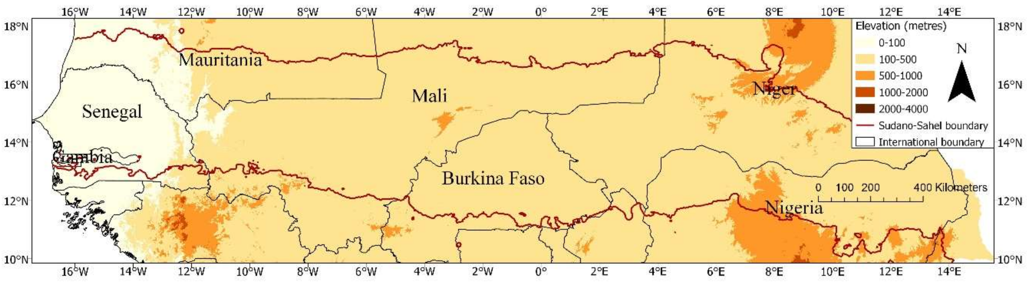
2.1. Study Area

Our study area consisted of the Sahelian and Sudanian savanna ecoregions of West Africa, bounded to the north by the Sahara Desert (MAP < 150 mm) and to the south by the Guinea savanna-forest mosaic (MAP > 900 mm), and extending from the Atlantic coast of Senegal and the Gambia on the west to the eastern borders of Niger and Nigeria on the east (Figure 1). The climate was strongly seasonal, with a unimodal distribution in annual rainfall that typically lasted from June to October and peaked in August of each year [35,36]. Vegetation in the area broadly reflected the climate gradient, ranging from dominantly herbaceous plant life with few trees and shrubs in the drier north, to woodland savannas in the south. The region is home to ~60 million people spread across parts of eight countries, with rural populations involved in combinations of subsistence agriculture and livestock (i.e., agro-pastoral) activities [37].

2.2. Retrieval and Preparation of Bioclimatic Data

We used the 3rd generation GIMMS NDVI dataset available in Google Earth Engine (GEE) to compute annual above-ground net primary productivity (ANPP) because of its reported temporal stability and overall good quality in semi-arid regions compared to other NDVI datasets of equal temporal coverage, such as the VIP and LTDR series [19]. GIMMS NDVI is derived from daily Advanced Very High Resolution Radiometer (AVHRR) multispectral reflectance and delivered as a semi-monthly (15 day) maximum NDVI global mosaic with a spatial resolution of 8 km [16]. Applying the associated quality flag filter (1 through 6, which included good, spline interpolated and average seasonal interpolated NDVI values), we retrieved all NDVI data for the years 1982–2013 covering our study area, with each layer resampled to a 0.05° pixel resolution to match the cell size of the rainfall data (described hereafter). For each pixel, monthly NDVI was determined as the maximum of the two semi-monthly values (to further minimize atmospheric effects), and the growing season cumulative NDVI (iNDVI, used as a proxy for ANPP) was calculated for each year by summing monthly values over a fixed wet month period (June–October). This summation was preceded by subtracting the mean NDVI of dry months (November–May) from each wet month value to normalize differences in dry season minima across the region [34] (Equation (1)) (Figure 2):

$$i\mathrm{NDVI}={\displaystyle \sum }_{June}^{October}\left(monthly NDVI-mean dry NDVI\right)$$

(1)

Rainfall data used in this study was obtained from the daily Climate Hazards Group Infrared Precipitation with Station (CHIRPS) dataset, which is derived from thermal infra-red measurements of cold cloud duration (CCD), locally calibrated into rainfall estimates (in mm), and further interpolated with station gauge data (using inverse distance weighting) to produce a comparatively high resolution (0.05° pixel size) and low latency product [38]. Using GEE, we retrieved daily rainfall (in mm) for the years 1982–2013 for our study area, and for each year, we calculated growing season cumulative rainfall (iRain) by summing over a fixed wet period (June 1st–October 31st, Equation (2), Figure 2). Although there were year-to-year differences in the exact timing of rainfall, the June-October period comfortably covered most, if not all, the precipitation in a given year for the Sahelian (2–3 months duration) and Sudanian (3–5 months duration) zones [36].

$$i\mathrm{Rain}={\displaystyle \sum }_{June 01}^{October 31}\left(daily rainfall in mm\right)$$

(2)

2.3. Modeling the Productivity–Rainfall Relationship

Rainfall is widely considered the primary driver of annual vegetation production in African savannas, and knowing the true shape of the productivity–rainfall relationship not only helps to provide a mechanistic explanation of observed vegetation trends, it is also fundamental to the use of concepts such as RUE and ResTrend [11]. Following in the footsteps of our prior watershed-scale study [34], we investigated the iNDVI–iRain relationship for the WASS regions using per-pixel ordinary least squares regression analysis between the time series of iRain (independent variable) and iNDVI (dependent variable used as proxy for ANPP). For each individual pixel, we fitted both a simple linear model (iNDVI vs. iRain, n = 32, α = 0.05) and a log-linear model (iNDVI vs. Ln[iRain], n = 32, α = 0.05). We believe both model specifications captured the broad sense of monotonic association, linear or saturating, between productivity and rainfall in West African savannas. We then used Akaike’s Information Criterion (AIC) [39] to evaluate the degree of support in the available data for either model. The model with the lowest AIC value was deemed to be the “best” representation of the productivity–rainfall relationship for that pixel.

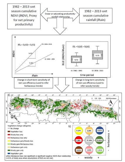
2.4. Assessing Overall Vegetation Trends and How They Are Influenced by the Model of the Cummulative Normalized Difference Vegetation Index–Cumulative Rainfall (iNDVI–iRain) Relationship

We used the ‘trends in residuals’ method (ResTrend) [26] to determine overall climate independent vegetation trends at each pixel location. Residuals in iNDVI were computed by subtracting the rainfall-predicted iNDVI from the observed iNDVI for each year. We then performed a linear regression of the residuals against time (in years). The ResTrend value (slope of the linear trend in residuals with time) was used to infer overall (non-specific) per-pixel vegetation trends. Positive values would indicate areas with productivity in later years increasingly exceeding rainfall-based expectations, while negative values indicate areas performing increasingly below expectations. To determine if the choice of the iNDVI-iRain model influenced the interpretation of trends, we performed the ResTrend analysis for two separate scenarios: (i) using residuals from the linear model, and (ii) using residuals from the “best” (AIC-selected) model, whether linear or log-linear.

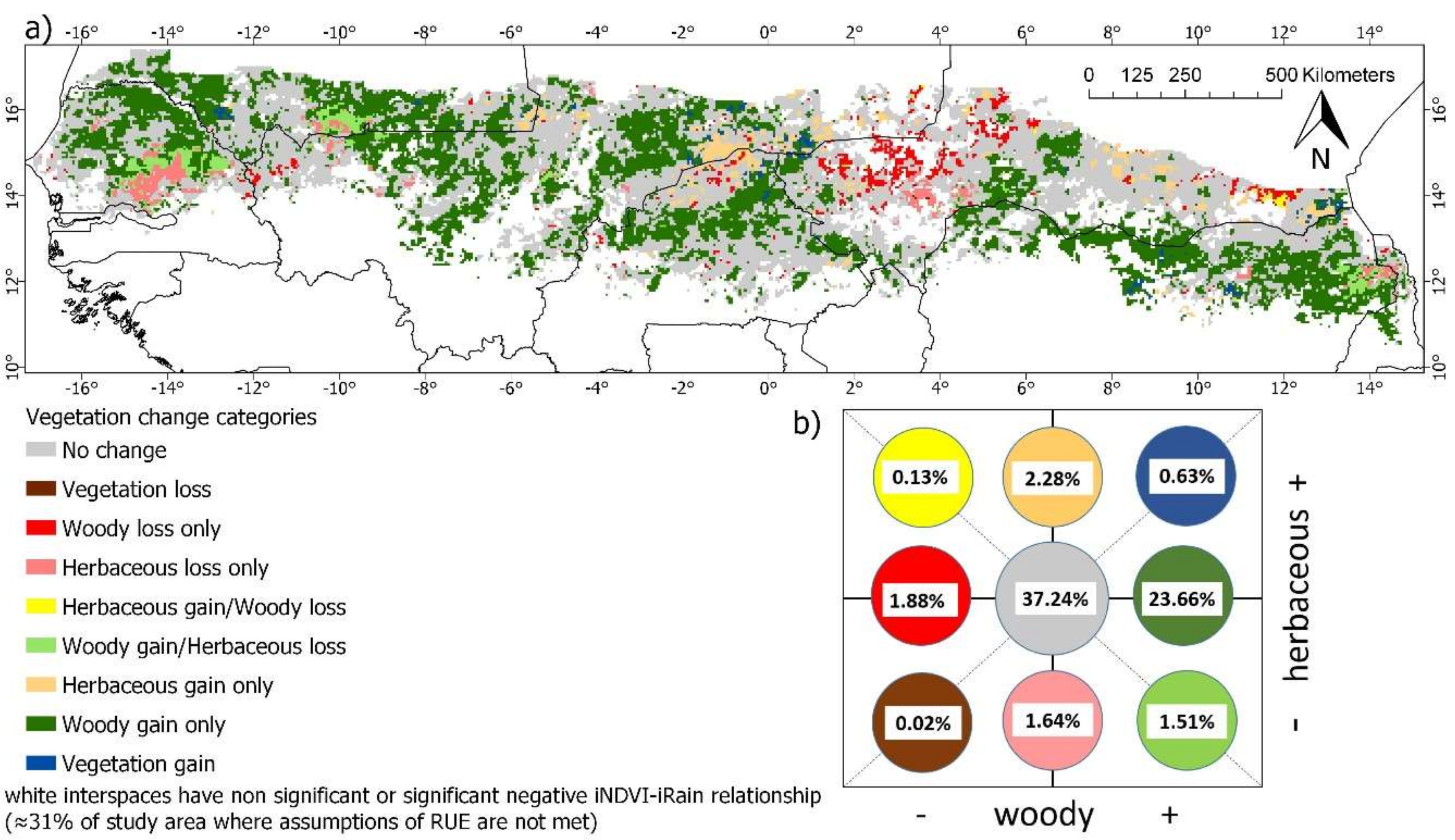
2.5. Diagnosing Trends in Woody and Herbaceous Components

To resolve overall vegetation trends into specific woody and herbaceous trends, we used a diagnostic approach that examined the sensitivity of productivity to long-term (decadal) and short-term (inter-annual) variability in rainfall (Figure 3). The conceptual framework is described in detail in our previous work [34] and summarized here: annual production of woody populations is relatively insensitive to inter-annual/short-term variability in rainfall, because leaf production on existing trees and shrubs depends largely on canopy architecture and stored reserves, while the density of woody plants in a landscape depends on the demographic processes of plant establishment and mortality that respond to climate and management over longer time-scales. This can be referred to as ‘long-term’ sensitivity (S_L), estimated as the mean RUE (i.e., mean of the ratio iNDVI/iRain) over an extended time-scale such as a decade. By contrast, the production of both annual and perennial grasses and herbaceous forbs is highly responsive to inter-annual variability in rainfall, and this ‘short-term’ sensitivity (S_S) can be estimated as the slope of the iNDVI-iRain relationship in a given period. By computing the difference in S_L and S_S between extended periods (i.e., δS_L and δS_S), it is possible to infer trends in the state of woody and herbaceous vegetation, respectively [34].

For this study we computed δS_L and δS_S between the first and last decades of our available time series: 1982–1991 and 2004–2013 (Figure 3). This was to allow for better contrast between the early and the more recent portion of the post-drought era, while still retaining sufficient data for statistical inference. δS_L was computed as the difference in decadal mean RUE, using a per-pixel independent t-test (RUE = iNDVI/iRain) (Figure 3b), while δS_S was computed using per-pixel analysis of covariance (ANCOVA) between two linear predictors of iNDVI: iRain and a binary time variable representing the two decades. In the latter case, the coefficient of the interaction term (iRain*time) measured “how differently” iNDVI responded to inter-annual variation in iRain in the last decade compared to the first (Figure 3a). In keeping with the third objective of this study, we also explored whether δS_L and δS_S values were influenced by the choice of the iNDVI-iRain model, linear or saturating. To do this, we additionally computed δS_L and δS_S for the “best” model scenario. This meant substituting iRain with its natural log value in all calculations of S_L and S_S at pixel locations determined (using iNDVI-iRain model AIC values) to have a better fit with the log-linear, as opposed to the linear, model.

2.6. Field Based Validation of Woody and Herbaceous Trends

We used in situ data on woody leaf and herbaceous biomass collected from field sites in Senegal from ~1987 to ~2017 to seek support for pixel-based vegetation trends (Supplementary Materials Figure S2). These sites were established in 1987 by the Centre de Suivi Ecologique (CSE) to be used for long-term monitoring of biomass. Woody leaf biomass and herbaceous biomass measurements are obtained at the end of each growing season along a 1 km transect located at each site. A detailed description of the field methods can be found in [40]. A total of 24 sites that have benefited from consistent data collection were used for our analysis. For each site, we determined separate woody leaf and herbaceous biomass trends (kgha⁻¹ year⁻¹) as the slope of the linear regression of biomass against time (in years). We then extracted the corresponding woody and herbaceous vegetation trends inferred from the analysis of the change in RUE sensitivity to determine, by comparison, if they were supported by the field data (Supplementary Materials Tables S1 and S3).

3. Results

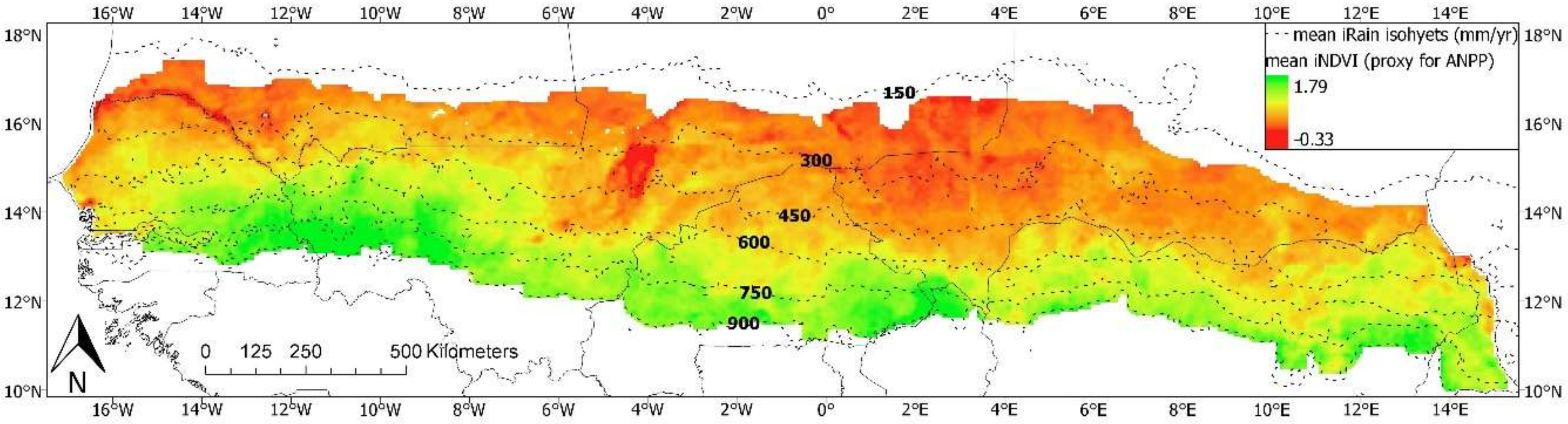
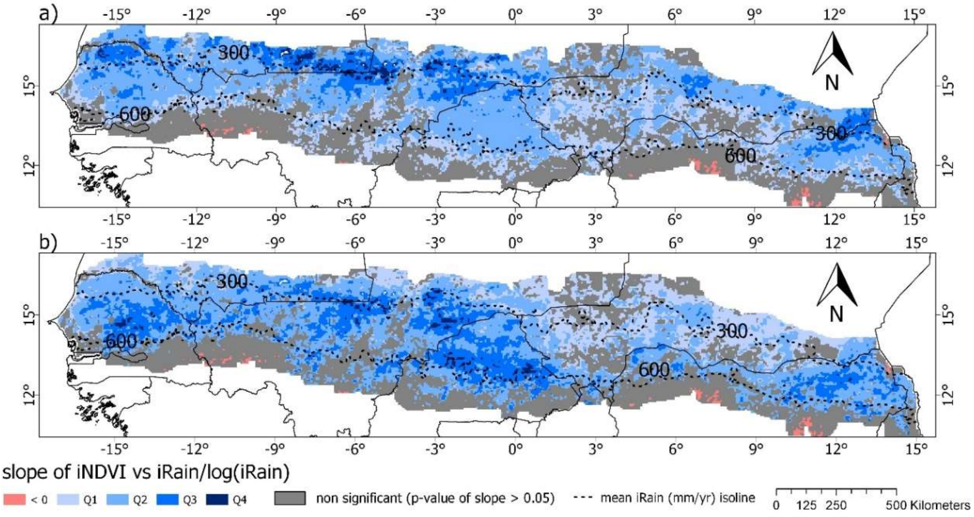
3.1. The Relationship between iNDVI and iRain in the West African Sudano-Sahelian (WASS) Region

Our first objective in this study was to re-examine how productivity, indexed here using iNDVI, varied with cumulative rainfall (iRain) in the semi-arid grasslands and savannas of the WASS region. We explored whether the long-term satellite and rainfall data for the region indicated a linear or saturating (log-linear) relationship between iNDVI and iRain. A close, positive relationship is anticipated in semi-arid and arid landscapes and is a necessary precursor for using changes in rain use efficiency as an indicator of long-term trends relating to post-drought recovery, or the degradation and recovery dynamics caused by climate variability and/or anthropogenic disturbance [11,34].

We found a significant positive linear relationship (p < 0.05) between iNDVI and iRain for most of the region (Figure 4a). Significant negative associations were rare and restricted to the southern fringes of the study area. Similar results were obtained for the relationship between iNDVI and the natural log value of iRain (Figure 4b), showing no consistent support for the use of either linear or log-linear models in the region if only statistical significance (p-value) and the direction of the relationship (positive or negative) are considered. However, the differences in spatial patterns of the linear and log-linear iNDVI-iRain models became more apparent when positive slope values from both models were compared after standardization into equal interval quarterly ranges (Figure 4). The results of the linear model revealed a distinct spatial pattern with the steepest slope values found mostly in the driest/northern part of the region (mean iRain of 300 mm or less), meanwhile areas showing the strongest saturating relationship (steepest slopes of iNDVI vs. Ln[iRain] model) extended across a greater latitudinal range and even into the wetter Sudanian zone (mean iRain of 600 mm or more, Figure 4b). More information on the patterns of the iNDVI-iRain relationship was revealed when we considered the best performing model at each location (model with lowest AIC value). Accordingly, 32% of pixels showed a preference for the linear model, 37% for the log-linear model, while 31% had negative or non-significant slopes (p > 0.05). The linear model again appeared to somewhat dominate the northern drier parts of the region, with the saturating function present throughout but more important in wetter, southern regions (Figure 5).

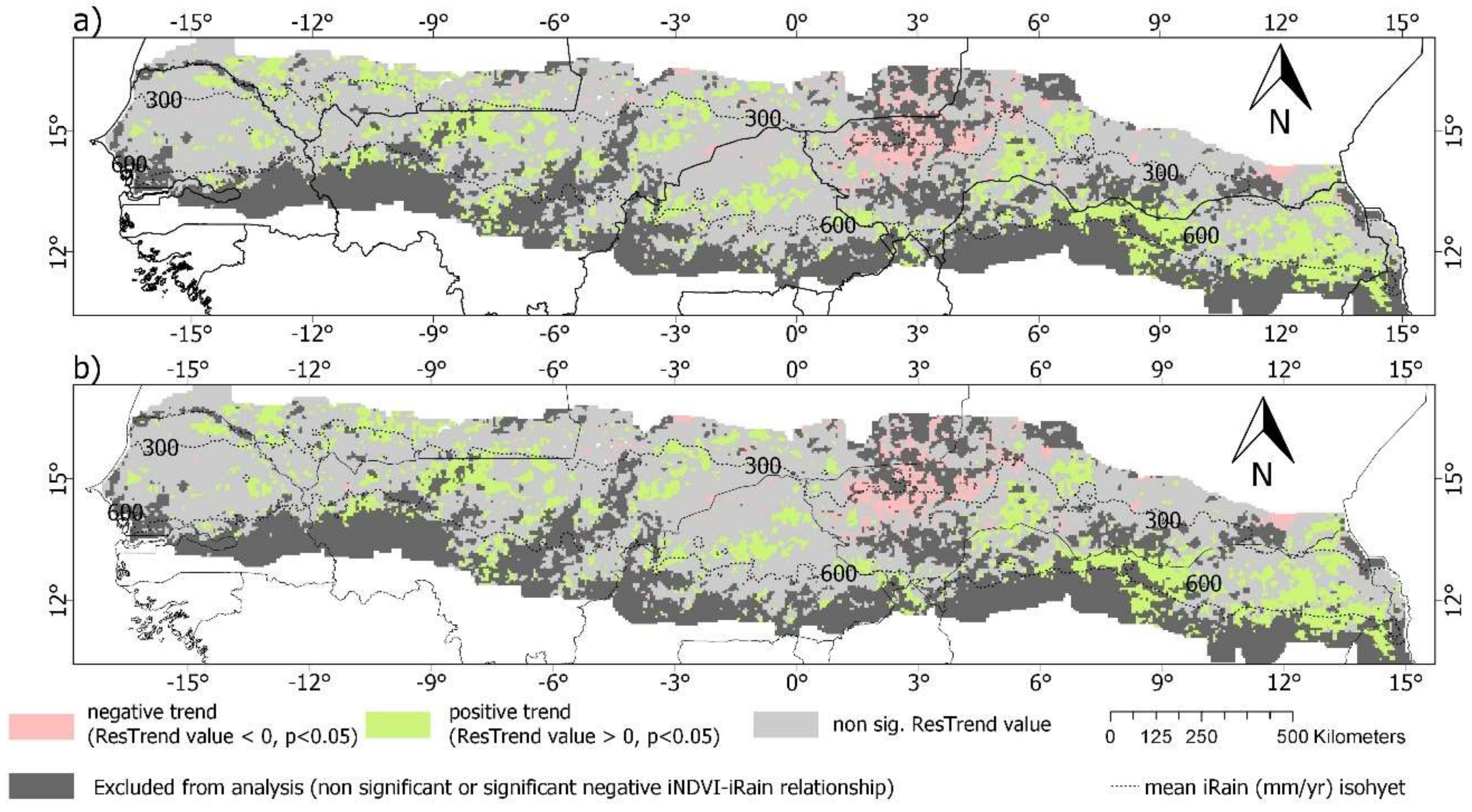
3.2. Overall Vegetation Trends Assessed Using the ResTrend Method

Having examined the nature of the iNDVI–iRain relationship for each pixel, our next objective was to assess per-pixel overall vegetation trends, using the ResTrend method, and to determine whether ResTrend results were impacted by the shape of the iNDVI–iRain relationship. Residuals are generally preferred to simply using RUE for vegetation trend analysis as the former are far less likely to be correlated with rainfall [11,27]. The annual residuals in iNDVI (observed iNDVI minus iNDVI predicted from model) were derived for both linear and log-linear models and analyzed for temporal trends indicating long-term increasing or decreasing RUE. Comparison of ResTrend results between the linear only and AIC-selected scenarios allowed us to identify locations where fitting a saturating function was important.

ResTrend analysis based on the linear iNDVI–iRain model showed that in ~17% of the area under study, the null hypothesis that the ResTrend value (slope of the iNDVI residuals versus time linear model) was not different from zero was rejected. Positive trends (ResTrend value > 0) accounted for ~14% of the total area and were spread across the region while negative trends (ResTrend value < 0) accounted for only ~3% of the whole region and were most noticeable in southwestern Niger (Figure 6). If we further disregard 31% of pixels that were excluded from ResTrend analysis for not meeting core RUE assumptions (Figure 5), the remainder (~52%) constituted areas with no significant long-term vegetation change outside of that caused by year-to-year rainfall variability. Furthermore, there was no noticeable difference in the abundance and the spatial patterns of significant positive or negative trends when comparing ResTrend results between the linear model (Figure 6a) and the best (AIC-selected) model scenarios (Figure 6b).

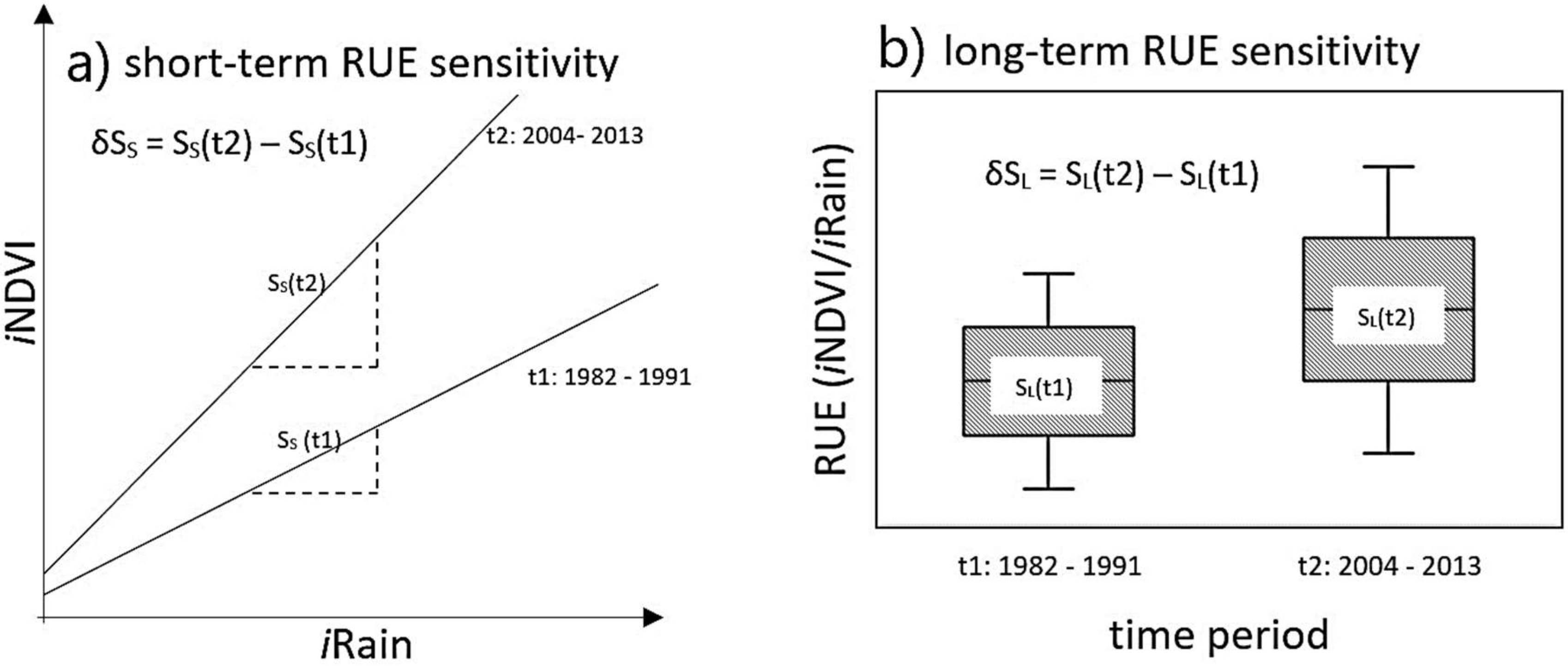
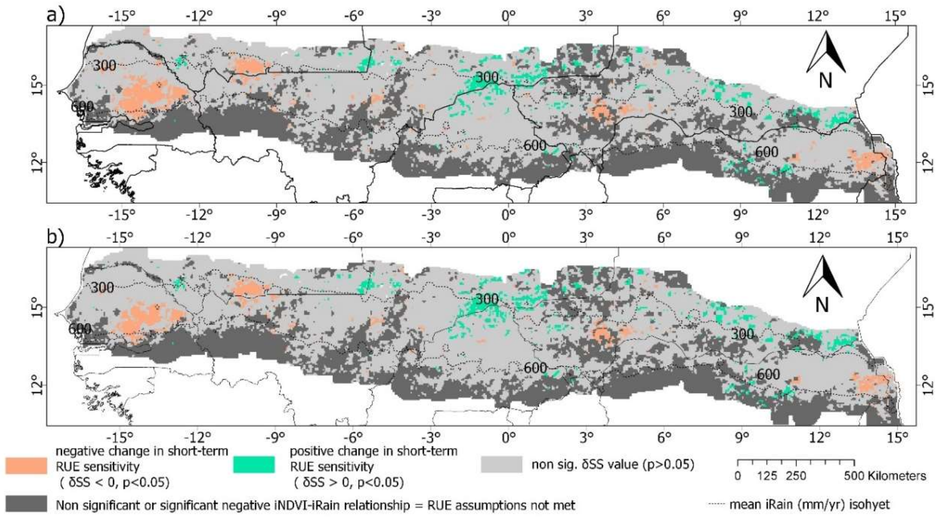
3.3. Long-Term and Short-Term Rain Use Efficiency (RUE) Sensitivity Analysis for Assessing Change in Specific Vegetation Types (Woody and Herbaceous)

While the results of the ResTrend analysis replicated earlier work [34,41] and provided information on the overall vegetation trends in the post-drought era, the approach did not allow any inference of the changes in the more specific vegetation components (woody or herbaceous) that were driving those trends. For this purpose, we analyzed the temporal changes in long-term and short-term RUE sensitivities (i.e., δS_L and δS_S, Figure 3) as indicators of change in woody and herbaceous components, respectively. Since this framework also relied on the underlying relationship between productivity and rainfall, we also assessed how δS_L and δS_S values were impacted by the form of the “best” iNDVI–iRain model for each location, substituting iRain with its natural log value in all instances where AIC model selection chose the log-linear over a linear relationship (see Figure 4).

Significant change in long-term RUE sensitivity across the region was dominated by positive trends (δS_L > 0), suggesting a significant increase in woody conditions when comparing the early and late periods within our time series of analysis (i.e., 1982–1991 versus 2004–2013) (Figure 7). As was seen with the results of the ResTrend analysis, southwestern Niger was a notable exception to the general trend, showing significant decrease in woody conditions. Unlike the ResTrend analysis, however, we found a notable difference in δS_L values when we considered the AIC-selected iNDVI–iRain model as opposed to just the linear model (Figure 7a,b). Under the linear relationship, where RUE was represented by the ratio of iNDVI/iRain, pixel locations with significant δS_L values (p < 0.05) were mostly restricted to the drier/northern half of the region (rarely occurring beyond a mean iRain isohyet of 600 mm), suggesting a trend of woody increase dominating the Sahel (Figure 7a). On the contrary, following model selection (i.e., replacing iRain where appropriate with its natural log in the calculation of δS_L), more locations in the wetter southern zones showed significant (and still mostly positive) δS_L values (Figure 7b), revealing a temporal increase in woody conditions even as you approach the mesic savannas where rainfall is less limiting.

Changes in short-term RUE sensitivity (δS_S), i.e., the difference in the iNDVI–iRain slope value between two decades, were comparatively less extensive (Figure 8), suggesting herbaceous dynamics play a lesser role in driving the long-term regional trends. We found instances of significant negative δS_S, suggesting long-term decrease in herbaceous production, in the central and eastern parts of Senegal, southern Mauritania, and parts of southwestern Niger. Meanwhile, the border region between Eastern Mali and Northern Burkina Faso and parts of southern-southeastern Niger had a noticeable concentration of positive δS_S, suggesting long-term increase in the production and cover of herbaceous vegetation. In contrast to results obtained for δS_L, the abundance and distribution of significant δS_S values remained pretty much the same whether assuming an all-linear iNDVI–iRain relationship model or using the AIC-selected model (Figure 8a,b).

To obtain a more complete and descriptive picture of long-term woody and herbaceous trends across the study area, we combined δS_L and δS_S values derived from the AIC-selected iNDVI–iRain model scenario into a single map (Figure 9a), with all possible combinations of simultaneous woody and herbaceous change represented in a simple 2D space (Figure 9b). Excluding areas that were not featured in the analysis due to assumptions of RUE not being met (~31%, Figure 5), the majority of pixels (~37%) did not show significant change in either woody or herbaceous vegetation conditions. Among the locations experiencing significant trends, woody gain only (i.e., with no significant change in the herbaceous community) was by far the most abundant category, accounting for almost a quarter (~24%) of the entire study area. Areas experiencing gain in herbaceous cover only (with no change in woody conditions) were a distant second in terms of abundance (~2.3%), closely followed by areas experiencing woody loss only (~1.9%), herbaceous loss only (~1.6%), and areas with woody increase (“encroachment”) associated with coincident decline in herbaceous vegetation (~1.5%). Areas with coincident losses in both woody and herbaceous vegetation were negligible (0.02%).

4. Discussion

4.1. The Nature of the Productivity–Rainfall Relationship in the Savannas of West Africa

The use of satellite-based metrics, such as iNDVI, as a proxy for ANPP, and the potential pitfalls associated with it are well established and must always be carefully considered [27,34,41]. Nevertheless, our results showing a strong positive association (slope) between iNDVI and iRain for the majority (69%, Figure 5) of the study area conform with the expectation that rainfall is the main driver of productivity in savannas, and is consistent with other satellite-based studies in the region [20,41]. A smaller but substantial part of the study area (31%) showed either null or negative association between productivity and cumulative rainfall. These areas are mostly concentrated, as expected, in the southern, wetter fringes of the region (with mean iRain > 600 mm, Figure 4 and Figure 5), where rainfall is less limiting and where other factors (e.g., light and nutrients) are presumed to be more limiting. Nevertheless, we also observed instances of a null or negative relationship in the northern, drier regions, such as in parts of central Mali and western Niger. This could be explained by confounding local conditions, for example, frequent flooding in the Niger delta area of central Mali and/or major land use change dynamics in other areas like Western Niger. Such drivers would impact local vegetation production more strongly than rainfall patterns [41].

In areas that indicated a significant positive iNDVI–iRain relationship, there was support in the data for both linear and saturating functions, with differences found only when model relative strength (standardized slope value, Figure 4) and model selection (AIC value, Figure 5) were considered. After AIC-based model selection, the saturating log-linear function was found to be slightly more common (37%) than the linear function (32%) across the region, no doubt due to the inclusion of the wetter Sudanian zone (600 mm < MAP < 900 mm) in the analysis. This also supports the idea of woody plants playing a relatively greater role in the observed long-term vegetation dynamics, since maximum woody cover is known to increase linearly with rainfall before saturating at approximately 650 mm MAP, after which canopy closure is possible [42]. Rainfall would have been highly limiting across the whole region in the immediate aftermath of the 1970s and early 1980s drought period, including the normally wetter Sudanian zone, due to the persistence of negative anomalies for the remainder of the 1980s (Supplementary Materials Figure S1) and the presumably low cover and density of plant communities that survived the drought. This supports the idea of an initial linear pattern of vegetation recovery, as woody plant communities responded strongly to the slowly increasing, though still below normal, rainfall levels. By the time annual rainfall had reached mostly positive anomaly levels (late 1990s and onwards, Figure S1), sufficient woody plant recovery might have already taken place in the wetter areas to induce a saturating effect.

4.2. Overall Vegetation Trends and How They Are Influenced by the Productivity–Rainfall Relationship

Our results from ResTrend analysis (Figure 6) provides evidence in support of overall post-drought vegetation trends across the region. As with our previous work [34], we found that taking into account the best productivity–rainfall model (linear or saturating) had little impact on the interpretation of trends in residuals (compare Figure 6a,b). Despite differences indicated by AIC values, both models were generally similar in terms of the sign (positive or negative) and significance (p-value) for most locations (Figure 4). It would make sense that they would produce similar trends in residuals. Our results revealed the significant post-drought trends to be mostly a greening phenomenon, consistent with the results of past ResTrend studies conducted in the region [41,43] and further dispelling the notion that the drought events of 70s/80s were part of a systematic shift towards desertification [8]. They also allude to the effect of possible beneficial land conservation practices such as agroforestry and erosion control [1,34]. Southwestern Niger was, however, a noticeable degradation hotspot, also consistent with the findings of past studies [27,32,41], and with the supposition that high density population centers such as Niamey (capital city of Niger), and their associated pressures on the surrounding landscape, may be offsetting the broader gains in natural vegetation across the region [44].

4.3. Trends in Woody/Herbaceous Vegetation Condition and How They Are Influenced by the Productivity–Rainfall Relationship

The results of our pixel-level analysis of long-term/short-term (i.e., woody/herbaceous) change in RUE sensitivity are consistent with our previous watershed-level study [34]. They reinforce findings of woody increase in the majority of watersheds sampled in northern Senegal and eastern Mali, as well as woody loss in those in southwestern Niger. However, the current study offers additional insight into regional level trends. The dominance of woody recovery in both the dry Sahel and the less dry Sudanian region (the latter did not feature prominently in our watershed-level analysis study), coupled with the sparse distribution of herbaceous trends, are examples of more detailed trends now being revealed. Another conclusion from this study is that woody “encroachment” (defined here as woody increase coupled with herbaceous decline), a well-known issue facing other drylands regions [45,46], does not appear to be a major phenomenon in West Africa (<2% of total area, Figure 9). Gains in woody conditions observed in this study were generally associated with little or no change in herbaceous conditions. This supports the view that the observed greening trends in West Africa over the past few decades may be primarily related to the recovery of woody populations following the reversal of drought conditions, rather than a fundamental shift in landscape functioning typically associated with shrub encroachment.

Other studies have attempted to analyze long-term trends in specific vegetation components in the WASS region, but these have been mostly undertaken, due to data constraints, under relatively shorter time scales (e.g., post-1990 or post-2000), making direct comparisons with our results difficult. However, there is a consistent indication that changes in woody vegetation are important in driving observed post-drought trends. For example, positive trends in field-measured woody leaf biomass were found to explain most of the satellite (NDVI)-based re-greening trends in northern Senegal [10]. Similarly, woody cover predicted from MODIS-based seasonality metrics for the years 2000–2014 showed strong patterns in eastern Senegal/western Mali (positive trends) and southwestern Niger/northern Nigeria (negative trends) [32]. Passive microwave vegetation optical depth (VOD) data were also used to show mostly positive woody trends in the Sahel region from early 1990s onwards, with subtle differences between the trends in stem/branch (VOD_wood) and leaf (VOD_leaf) woody plant components [33]. However, it should be noted that the exact locations of positive and negative woody trends observed in the aforementioned studies did not always agree with our analysis, possibly due to differences in data, methods, and time frame of analysis. For example, the woody cover trends determined in [32] for northern Nigeria, eastern Senegal/western Mali and eastern Mali were mostly contrary to our results. We also found that our change in long-term RUE-sensitivity (δS_L, used to infer woody trends) agreed more with trends in woody leaf biomass (VOD_leaf) than with trends in wood biomass (VOD_wood), as determined in [33], likely due to our use of NDVI (‘greenness’) for measuring productivity and RUE.

Independent validation of long-term woody/herbaceous vegetation trends assessed through remote sensing is a challenging task, especially in West Africa where there is a paucity of long-term field data records. More so, due to the typical structure of savanna landscapes (i.e., scattered small trees and shrubs mixed with open grassland), comparatively higher resolution remote sensing data with adequate historical coverage such as Landsat imagery is rather insufficient in accurately separating historical woody and herbaceous vegetation cover for validation purposes. Our own attempts to validate pixel trends with in situ data from Senegal led to mixed results. Based on the sign (+/−) and significance (p-value) of field biomass trends, we found that a majority of field sites agreed with pixel-based trends in herbaceous vegetation (77% of 22 sites) while only half of field sites agreed with woody vegetation tendencies (50% of 22 sites) (Supplementary Materials Table S1). This was also evident when we compared mean woody leaf and herbaceous biomass trends across pixel categories (Supplementary Materials Figure S3). We recognize that the difference in scale (1 km field transect versus ~5.6 km/0.05° pixel dimension), coupled with the use of a transect method for field data collection (arguably more suitable for sampling the evenly distributed herbaceous vegetation), may have contributed to the lesser support for pixel-based woody trends in the field data. We also note that some pixel-based trend categories were not well represented in the field data, which weakened our efforts at validation. Nevertheless, the mostly positive woody leaf biomass trends and the mostly non-significant herbaceous biomass trends reflect the general picture of this small part of the region as presented by the pixel-level RUE change analysis (Supplementary Materials Figure S2).

A key improvement in this study over prior analyses was the determination of whether the nature (linear or saturating) of the productivity–rainfall relationship had any effect on the inferred woody and herbaceous trends. One interesting result from this was the effect on assessing woody trends, specifically through detection of more significant, and mostly positive, trends in the wetter Sudanian areas (Figure 7b). Normally, the saturating effect of high rainfall suppresses RUE, indicating that other limiting factors such as light and nutrient availability could be becoming more important. However, by accounting for a log-linear function where appropriate, the study revealed that recovery of woody vegetation was not restricted to the drier Sahel, as was indicated by the “linear only” scenario (Figure 7a), but has been an important, and perhaps dominant, part of the re-greening trend across the whole region since the 1970s and 1980s droughts.

A limitation of this study is that the relatively short time series may have influenced our ability to detect significant trends at some pixel locations. We also acknowledge that our analysis did not account for other important biophysical parameters, such as long-term changes in the richness and abundance of specific woody and herbaceous plant species that could be of local ecological and/or socio-economic importance. We therefore recommend that this study be followed up with more detailed studies that would further characterize the woody and herbaceous trends determined by our analysis, as well as investigate potential local-level drivers of trends, natural and/or anthropogenic.

5. Conclusions

Satellite-based evidence of post-drought vegetation recovery across West African savannas has been well documented [9,27,40,45]. However, earlier studies have mostly focused on assessing overall re-greening or degradation trends, with little attention given to the underlying trends in separate woody and herbaceous components. In this study we revisited the discussion on long-term vegetation trends in water-limited environments, and we used our previously developed framework for diagnosing pixel-level trends in woody and herbaceous vegetation in the WASS region. This framework is based on how vegetation productivity responds to rainfall on inter-annual and inter-decadal time-scales.

Our results are consistent with what is known for drylands, with mostly strong, positive relationships between productivity and rainfall, which become less pronounced at higher rainfall levels. We found that the choice of productivity–rainfall functional model (linear or saturating) had little or no impact on the ability to infer overall vegetation trends determined using ResTrend analysis or the more specific herbaceous trends determined using a change in the inter-annual response of productivity to rainfall (short term RUE sensitivity). However, model selection was important for the inference of woody vegetation trends diagnosed using decadal-scale changes in RUE sensitivity, in which case significant woody trends were detected not only in the dry Sahel zone but also in the less dry Sudanian zone. We conclude that, except for southwestern Niger, long-term re-greening trends across the WASS region are dominated by increase in woody vegetation, suggesting a steady recovery of woody populations in the aftermath of the 1970s and 1980s drought.

The outcome of this study provides inroads into understanding important aspects of post-drought vegetation dynamics in the WASS region, by partitioning recovery or degradation labels into more detailed trends in woody and herbaceous functional groups. This more detailed analysis has profound implications for assessing patterns of ecological functioning and sustainability across the region, where woody and herbaceous plant communities provide distinct suites of ecosystem services. Long-term assessments of this kind will be critical in the Sahel and other dryland regions as they respond to climate variability, long-term climate change, and changing anthropogenic influences.

References

1. Hanan, N.P. Agroforestry in the Sahel. Nat. Geosci. 2018, 11, 296. [Google Scholar] [CrossRef]
2. Wezel, A.; Lykke, A.M. Woody vegetation change in Sahelian West Africa: Evidence from local knowledge. Environ. Dev. Sustain. 2006, 8, 553–567. [Google Scholar] [CrossRef]
3. Dovie, D.B.K.; Shackleton, C.M.; Witkowski, E.T.F. Conceptualizing the human use of wild edible herbs for conservation in South African communal areas. J. Environ. Manag. 2007, 84, 146–156. [Google Scholar] [CrossRef] [PubMed]
4. Ludwig, J.A.; Wilcox, B.P.; Breshears, D.D.; Tongway, D.J.; Imeson, A.C. Vegetation patches and runoff–erosion as interacting ecohydrological processes in semiarid landscapes. Ecology 2005, 86, 288–297. [Google Scholar] [CrossRef]
5. Russo, R.O. Agrosilvopastoral systems: A practical approach toward sustainable agriculture. J. Sustain. Agric. 1996, 7, 5–16. [Google Scholar] [CrossRef]
6. Sala, O.E.; Parton, W.J.; Joyce, L.A.; Lauenroth, W.K. Primary production of the central grassland region of the United States. Ecology 1988, 69, 40–45. [Google Scholar] [CrossRef]
7. Charney, J.G. Dynamics of deserts and drought in the Sahel. Q. J. R. Meteorol. Soc. 1975, 101, 193–202. [Google Scholar] [CrossRef]
8. Nicholson, S.E.; Tucker, C.J.; Ba, M.B. Desertification, drought and surface vegetation: An example from the West African Sahel. Bull. Am. Meteorol. Soc. 1998, 79, 815–830. [Google Scholar] [CrossRef]
9. Anyamba, A.; Tucker, C.J. Analysis of Sahelian vegetation dynamics using NOAA-AVHRR NDVI data from 1981–2003. J. Arid Environ. 2005, 63, 596–614. [Google Scholar] [CrossRef]
10. Brandt, M.; Mbow, C.; Diouf, A.A.; Verger, A.; Samimi, C.; Fensholt, R. Ground and satellite-based evidence of the biophysical mechanisms behind the greening Sahel. Glob. Chang. Biol. 2015, 21, 1610–1620. [Google Scholar] [CrossRef]
11. Dardel, C.; Kergoat, L.; Hiernaux, P.; Grippa, M.; Mougin, E.; Ciais, P.; Nguyen, C.-C. Rain-use-efficiency: What it tells us about the conflicting Sahel greening and Sahelian paradox. Remote Sens. 2014, 6, 3446–3474. [Google Scholar] [CrossRef]
12. Charney, J.; Stone, P.H.; Quirk, W.J. Drought in the Sahara: A biogeophysical feedback mechanism. Science 1975, 187, 434–435. [Google Scholar] [CrossRef] [PubMed]
13. Eklundh, L.; Olsson, L. Vegetation index trends for the African Sahel 1982–1999. Geophys. Res. Lett. 2003, 30, 1430. [Google Scholar] [CrossRef]
14. Herrmann, S.M.; Anyamba, A.; Tucker, C.J. Recent trends in vegetation dynamics in the African Sahel and their relationship to climate. Glob. Environ. Chang. 2005, 15, 394–404. [Google Scholar] [CrossRef]
15. Tucker, C.J. Red and photographic infrared linear combinations for monitoring vegetation. Remote Sens. Environ. 1979, 8, 127–150. [Google Scholar] [CrossRef]
16. Tucker, C.J.; Pinzon, J.E.; Brown, M.E.; Slayback, D.A.; Pak, E.W.; Mahoney, R.; Vermote, E.F.; Saleous, N.E. An extended AVHRR 8 km NDVI dataset compatible with MODIS and SPOT vegetation NDVI data. Int. J. Remote Sens. 2005, 26, 4485–4498. [Google Scholar] [CrossRef]
17. Didan, K. NASA MEaSUREs vegetation index and phenology (VIP) vegetation indices monthly global 0.05Deg CMG. NASA EOSDIS Land Process. DAAC 2016, 4. [Google Scholar] [CrossRef]
18. Pedelty, J.; Devadiga, S.; Masuoka, E.; Brown, M.; Pinzon, J.; Tucker, C.; Vermote, E.; Prince, S.; Nagol, J.; Justice, C.; et al. Generating a long-term land data record from the AVHRR and MODIS Instruments. In Proceedings of the 2007 IEEE International Geoscience and Remote Sensing Symposium, Barcelona, Spain, 23–28 July 2007; pp. 1021–1025. [Google Scholar]
19. Tian, F.; Brandt, M.; Liu, Y.Y.; Verger, A.; Tagesson, T.; Diouf, A.A.; Rasmussen, K.; Mbow, C.; Wang, Y.; Fensholt, R. Remote sensing of vegetation dynamics in drylands: Evaluating vegetation optical depth (VOD) using AVHRR NDVI and in situ green biomass data over West African Sahel. Remote Sens. Environ. 2016, 177, 265–276. [Google Scholar] [CrossRef]
20. Fensholt, R.; Proud, S.R. Evaluation of earth observation based global long-term vegetation trends—Comparing GIMMS and MODIS global NDVI time series. Remote Sens. Environ. 2012, 119, 131–147. [Google Scholar] [CrossRef]
21. Didan, K. MOD13C2 MODIS/Terra vegetation indices monthly L3 global 0.05 deg CMG V006. NASA EOSDIS Land Process. DAAC 2015, 10. [Google Scholar] [CrossRef]
22. Verhegghen, A.; Bontemps, S.; Defourny, P. A global NDVI and EVI reference data set for land-surface phenology using 13 years of daily SPOT-VEGETATION observations. Int. J. Remote Sens. 2014, 35, 2440–2471. [Google Scholar] [CrossRef]
23. Tucker, C.J.; Newcomb, W.W.; Los, S.O.; Prince, S.D. Mean and inter-year variation of growing-season normalized difference vegetation index for the Sahel 1981–1989. Int. J. Remote Sens. 1991, 12, 1133–1135. [Google Scholar] [CrossRef]
24. Nicholson, S.E.; Davenport, M.L.; Malo, A.R. A comparison of the vegetation response to rainfall in the Sahel and East Africa, using normalized difference vegetation index from NOAA AVHRR. Clim. Chang. 1990, 17, 209–241. [Google Scholar] [CrossRef]
25. Bai, Z.G.; Dent, D.L.; Olsson, L.; Schaepman, M.E. Proxy global assessment of land degradation. Soil Manag. 2008, 24, 223–234. [Google Scholar] [CrossRef]
26. Evans, J.; Geerken, R. Discrimination between climate and human-induced dryland degradation. J. Arid Environ. 2004, 57, 535–554. [Google Scholar] [CrossRef]
27. Fensholt, R.; Rasmussen, K.; Kaspersen, P.; Huber, S.; Horion, S.; Swinnen, E. Assessing land degradation/recovery in the African Sahel from long-term earth observation based primary productivity and precipitation relationships. Remote Sens. 2013, 5, 664–686. [Google Scholar] [CrossRef]
28. Wessels, K.J. Comments on ‘Proxy global assessment of land degradation’ by Bai et al. (2008). Soil Use Manag. 2009, 25, 91–92. [Google Scholar] [CrossRef]
29. Hiernaux, P.; Diarra, L.; Trichon, V.; Mougin, E.; Soumaguel, N.; Baup, F. Woody plant population dynamics in response to climate changes from 1984 to 2006 in Sahel (Gourma, Mali). J. Hydrol. 2009, 375, 103–113. [Google Scholar] [CrossRef]
30. Hiernaux, P.; Mougin, E.; Diarra, L.; Soumaguel, N.; Lavenu, F.; Tracol, Y.; Diawara, M. Sahelian rangeland response to changes in rainfall over two decades in the Gourma region, Mali. J. Hydrol. 2009, 375, 114–127. [Google Scholar] [CrossRef]
31. Brandt, M.; Verger, A.; Diouf, A.A.; Baret, F.; Samimi, C. Local vegetation trends in the Sahel of Mali and senegal using long time series FAPAR satellite products and field measurement (1982–2010). Remote Sens. 2014, 6, 2408–2434. [Google Scholar] [CrossRef]
32. Brandt, M.; Hiernaux, P.; Rasmussen, K.; Mbow, C.; Kergoat, L.; Tagesson, T.; Ibrahim, Y.Z.; Wélé, A.; Tucker, C.J.; Fensholt, R. Assessing woody vegetation trends in Sahelian drylands using MODIS based seasonal metrics. Remote Sens. Environ. 2016, 183, 215–225. [Google Scholar] [CrossRef]
33. Tian, F.; Brandt, M.; Liu, Y.Y.; Rasmussen, K.; Fensholt, R. Mapping gains and losses in woody vegetation across global tropical drylands. Glob. Chang. Biol. 2017, 23, 1748–1760. [Google Scholar] [CrossRef] [PubMed]
34. Kaptué, A.T.; Prihodko, L.; Hanan, N.P. On regreening and degradation in Sahelian watersheds. Proc. Natl. Acad. Sci. 2015, 112, 12133–12138. [Google Scholar] [CrossRef] [PubMed]
35. Nicholson, S.E.; Webster, P.J. A physical basis for the interannual variability of rainfall in the Sahel. Q. J. R. Meteorol. Soc. 2007, 133, 2065–2084. [Google Scholar] [CrossRef]
36. Nicholson, S.E. The West African Sahel: A Review of Recent Studies on the Rainfall Regime and Its Interannual Variability. Available online: https://www.hindawi.com/journals/isrn/2013/453521/ (accessed on 19 February 2019).
37. Backgrounder on the Sahel, West Africa’s Poorest Region. Available online: http://www.irinnews.org/feature/2008/06/02 (accessed on 31 August 2018).
38. Funk, C.; Peterson, P.; Landsfeld, M.; Pedreros, D.; Verdin, J.; Shukla, S.; Husak, G.; Rowland, J.; Harrison, L.; Hoell, A.; et al. The climate hazards infrared precipitation with stations—A new environmental record for monitoring extremes. Sci. Data 2015, 2, 150066. [Google Scholar] [CrossRef] [PubMed]
39. Akaike, H. A new look at the statistical model identification. IEEE Trans. Autom. Control 1974, 19, 716–723. [Google Scholar] [CrossRef]
40. Diouf, A.A.; Brandt, M.; Verger, A.; Jarroudi, M.E.; Djaby, B.; Fensholt, R.; Ndione, J.A.; Tychon, B. Fodder biomass monitoring in Sahelian rangelands using phenological metrics from FAPAR time series. Remote Sens. 2015, 7, 9122–9148. [Google Scholar] [CrossRef]
41. Leroux, L.; Bégué, A.; Lo Seen, D.; Jolivot, A.; Kayitakire, F. Driving forces of recent vegetation changes in the Sahel: Lessons learned from regional and local level analyses. Remote Sens. Environ. 2017, 191, 38–54. [Google Scholar] [CrossRef]
42. Sankaran, M.; Hanan, N.P.; Scholes, R.J.; Ratnam, J.; Augustine, D.J.; Cade, B.S.; Gignoux, J.; Higgins, S.I.; Le Roux, X.; Ludwig, F.; et al. Determinants of woody cover in African savannas. Nature 2005, 438, 846–849. [Google Scholar] [CrossRef]
43. Fensholt, R.; Langanke, T.; Rasmussen, K.; Reenberg, A.; Prince, S.D.; Tucker, C.; Scholes, R.J.; Le, Q.B.; Bondeau, A.; Eastman, R.; et al. Greenness in semi-arid areas across the globe 1981–2007—An earth observing satellite based analysis of trends and drivers. Remote Sens. Environ. 2012, 121, 144–158. [Google Scholar] [CrossRef]
44. Brandt, M.; Rasmussen, K.; Peñuelas, J.; Tian, F.; Schurgers, G.; Verger, A.; Mertz, O.; Palmer, J.R.B.; Fensholt, R. Human population growth offsets climate-driven increase in woody vegetation in sub-Saharan Africa. Nat. Ecol. Evol. 2017, 1, 0081. [Google Scholar] [CrossRef] [PubMed]
45. Eldridge, D.J.; Bowker, M.A.; Maestre, F.T.; Roger, E.; Reynolds, J.F.; Whitford, W.G. Impacts of shrub encroachment on ecosystem structure and functioning: Towards a global synthesis. Ecol. Lett. 2011, 14, 709–722. [Google Scholar] [CrossRef] [PubMed]
46. Roques, K.G.; O′Connor, T.G.; Watkinson, A.R. Dynamics of shrub encroachment in an African savanna: Relative influences of fire, herbivory, rainfall and density dependence. J. Appl. Ecol. 2001, 38, 268–280. [Google Scholar] [CrossRef]
Figure 1. Map of the West African Sudano-Sahelian (WASS) region.
Remotesensing 11 00576 g001
Figure 2. Summary of bioclimatic data used in the study: cumulative wet season normalized difference vegetation index (NDVI) (iNDVI—used as an index of aboveground net primary productivity) and annual wet season rainfall integral (iRain). Values displayed are means for 32 years (1982–2013). See Supplementary Materials for links to Google Earth Engine codes used to prepare time series data.
Remotesensing 11 00576 g002
Figure 3. Conceptual framework for diagnosing per-pixel trends in separate woody and herbaceous vegetation (see [34] for details). (a) Change in short-term rain use efficiency (RUE) sensitivity (δSS) is the difference in slope (SS) of the iNDVI/iRain relationship between 2 periods (t1, t2). δSS is used to infer changes in herbaceous vegetation that responds rapidly to inter-annual variability in rainfall. (b) Change in long-term RUE sensitivity (δSL) is the difference in long-term mean of the ratio iNDVI/iRain between t1 and t2 and is used to infer changes in woody community density and cover, which generally changes slowly as a function of demographic processes (recruitment, growth, and mortality). At locations where there is a preference for a saturating productivity–rainfall relationship, iRain is replaced in the above framework by Ln[iRain].
Remotesensing 11 00576 g003
Figure 4. Relationship between iNDVI and iRain: (a) linear model, (b) log-linear model. To facilitate direct comparisons of linear and log scale, positive slope values from both models have been classified using equal interval ranges from Q1(lowest quarter—significant but weakest relationship) to Q4 (highest quarter—significant and strongest relationship).
Remotesensing 11 00576 g004
Figure 5. (a) Map showing “best” per-pixel iNDVI–iRain relationship selected using Akaike Information Criterion (AIC) values of competing models. (b) Pie chart showing distribution of pixels according to the selected model. Grey colored pixels are locations with fitted slopes not significantly different from zero (p > 0.05) in either model (or in a few cases, locations with significant negative slopes). In these areas, assumptions of the rain use efficiency approach are not met with our data and, thus, they are excluded from trend analysis.
Remotesensing 11 00576 g005
Figure 6. Nonspecific vegetation trends (1982–2013) in the WASS region based on trends in the residuals of iNDVI–iRain relationships: (a) trends based on residuals from linear model only, (b) trends based on residuals of the best model determined by AIC (linear or log-linear). The similarity between both figures shows that choosing the best model had no discernible effect on the sign (+/−) and significance (p-value < 0.05) of ResTrend values, consistent with was found during previous watershed scale analysis [34].
Remotesensing 11 00576 g006
Figure 7. Inter-decadal change in long-term RUE sensitivity (δSL): (a) assuming a linear iNDVI–iRain relationship, (b) following AIC model-selection between linear and saturating relationships.
Remotesensing 11 00576 g007
Figure 8. Inter-decadal change in short-term RUE sensitivity (δSS: change in the slope of iNDVI-iRain relationship): (a) assuming a linear iNDVI–iRain relationship, (b) following AIC model-selection between linear and saturating relationships.
Remotesensing 11 00576 g008
Figure 9. Concurrent woody and herbaceous vegetation changes between the 1982–1991 and 2004–2013 decades in the WASS region based on δSL and δSS values derived assuming the best (AIC-selected) productivity-rainfall relationship at each location. (a) Map of vegetation change categories, (b) Chart showing conceptual position and the relative abundance of each category in a 2-D space. Both figures share the same color legend.
Remotesensing 11 00576 g009