Predicting Rice Grain Yield Based on Dynamic Changes in Vegetation Indexes during Early to Mid-Growth Stages

Abstract

Predicting the grain yield during early to mid-growth stages is important for initial diagnosis of rice and quantitative regulation of topdressing. In this study, we conducted four experiments using different nitrogen (N) application rates (0–400 kg N∙ha⁻¹) in three Japonica rice cultivars (Wuyunjing24, Ningjing4, and Lianjing7) grown in Jiangsu province, Eastern China, from 2015–2016. Spectral reflectance data were collected multiple times during early to mid-growth stages using an active mounted sensor (RapidScan CS-45, Holland Scientific Inc., Lincoln, NE, USA). Data were then used to calculate optimal vegetation indexes (normalized difference red edge, NDRE; normalized difference vegetation index, NDVI; ratio vegetation index, RVI; red-edge ratio vegetation index, RERVI), which were used to develop a dynamic change model and in-season grain yield prediction model. The NDRE index was more stable than other indexes (NDVI, RVI, RERVI), showing less standard deviation at the same N fertilizer rate. The R² of the relationships between leaf area index (LAI), plant nitrogen accumulation (PNA), and NDRE also increased compared to other indexes. These findings suggest that NDRE is suitable for analysis of paddy rice N nutrition. According to real-time series changes in NDRE, the resulting dynamic model followed a sigmoid curve, with a coefficient of determination (R²) >0.9 and relative root-mean-square error <5%. Moreover, the feature platform value (saturation value, SV) of the NDRE-based model accurately predicted the differences between treatments and the final grain yield levels. R² values of the relationship between SV and yield were >0.7. For every 0.1 increase in SV, grain yield increased by 3608.1 kg·ha⁻¹. Overall, our new dynamic model effectively predicted grain yield at stem elongation and booting stages, providing real-time crop N nutrition data for management of N fertilizer topdressing in rice production.

1. Introduction

Rice (Oryza sativa L.) is a staple food for billions of people worldwide. China is the largest rice producer in the world, with approximately 31 million hectares of paddy rice cultivation [1]. To ensure sustainable food production, agricultural producers invest in a significant amount of nitrogen (N) fertilizer [1]. Zhang et al. reported that the N use efficiency (NUE) of China’s major food crops was less than 30% [2], representing 33% of the global NUE, and 40% of that in developed countries in Europe and America [3]. Scientific management of N fertilizer use is, therefore, crucial in realizing the goals of high yield, quality, and efficiency in rice production in eastern China.

Methods based on appropriate indicators, such as leaf area index (LAI), soil and plant analyzer development (SPAD), and N nutrition index (NNI), and yield forecasts are often used for crop growth diagnostics and fertilizer quantification [4]. Site-specific nutrient management (SSNM) of N fertilizer topdressing, which is based on comparisons of SPAD and threshold values at key growth stages, is one such method [5]. However, different varieties have different thresholds. For example, SPAD thresholds of rice cultivars Shanyou63 and Liangyoupei9 were found to be 36 and 38, respectively [6,7]. During rice-wheat rotation, SPAD values should be more than 37.5 to ensure high yield; if lower, 30 kg∙ha⁻¹ N fertilizer topdressing is applied [8]. Meanwhile, Qiong et al. recommended an SPAD threshold of 39–41 for the application of N fertilizer at critical growth stages in paddy rice [9] (

Table 1. Summary of threshold distributions under different conditions.

Author	Eco-site	Variety	Threshold
Huang et al. [6]	Hubei, China	Shanyou63, Liangyoupei9	36, 38
Singh et al. [7]	Indo-Gangetic plains, India	PR118, PAU201, etc.	37.5
Qiong et al. [8]	Hubei, China	Peiliangyou3076, Yangliangyou6	39–41
He et al. [3]	Hubei, China	Liangyoupei9, Shanyou63	38, 39, 35–37
Fan et al. [10]	Helongjiang, China	Songjing98-128	38–40

). Moreover, Peng et al. suggested that, under SSNM management in China, a plot requires just 68% of the N fertilizer applied under traditional fertilization methods, resulting in a 5% increase in N use efficiency (NUE) [5]. However, SPAD thresholds are affected by a number factors including the species, regional climates, soil type, and N fertilizer management measures [7], resulting in significantly different thresholds.

The critical N dilution curve can also be used to describe in-season plant N status [11]. Based on this model, the N nutrition index (NNI), a widely applicable diagnostic indicator, is used for N diagnosis [12]. When NNI = 1, N nutrition is optimal, while NNI > 1 and NNI < 1 indicate excess and deficient N nutrition, respectively [13]. NNI can accurately predict the relative yield of rice at different stages, with coefficients of determination (R²) greater than 0.74 [14]. Similar results were also obtained using the normalized difference vegetation index (NDVI) of GreenSeeker (Trimble Navigation Ltd. Sunnyvale, CA, USA) in barley and maize. NNI was previously found to account for 70% of the variation in crop N nutrition [15,16]; however, in practical applications, in different regions and with different rice varieties, NNI is less effective. Calculated NNI values were found to have a large range [17]. For example, Hu et al. reported NNI values ranging from 0.4–1.6 [18], while Houlès et al. suggested that 0.25–1.25 was the optimal range [19]. Moreover, Debaeke et al. revealed NNI values ranging from 0.5–1.5 in wheat [20]. Significant differences between studies were also revealed [21]. These differences in critical N concentrations, therefore, reduced the popularity and widespread use of NNI.

Yield prediction methods use crop conditions at early to mid-growth stages to predict the potential yield of that season, thereby determining the amount of fertilizer topdressing required [4]. In traditional methods, agronomic parameters such as the leaf area index (LAI) and plant dry matter (PDM) at different growth stages are commonly used to predict potential yield. The quantitative relationships between these indicators and final yield is then determined, allowing N fertilizer application rates to be recommended [22]. Portable spectral sensors are also used to collect crop spectral information, which is then used to determine vegetation indexes and the relationship with final yield. Moreover, Spitkó et al. revealed a relationship between NDVI and yield after anthesis; however, the correlation coefficient was less than 0.5 (r) [23]. Tubaña et al. also established a relationship between relative NDVI and relative yield (relative to the respective maximum) at panicle differentiation and for two weeks thereafter [24]. Similarly, the determination coefficient was less than 0.5. Meanwhile, Liu et al. confirmed a relatively stable relationship between NDVI and grain yield in double-cropping rice during major growth periods, with R² values ranging from 0.6 to 0.65 [25].

Xue et al. also described the relationship between NDVI and N accumulation from tillering to early grain filling stages, and used the obtained sufficiency index (SI) to predict potential yield and guide topdressing nitrogen management [26]. The R² value was 0.8, resulting in effective improvements in NUE. Furthermore, Evert et al. studied the relationship between the weighted difference vegetation index (WDVI) and the N status of potato using MSR87 (CropScan Inc., Rochester, MN, USA) [27], revealing a significant correlation between WDVI and N uptake. Accordingly, they were able to establish a potential yield model for potato. Similarly, Morier et al. used FieldSpec HandHeld (Analytical Spectral Devices (ASD), Inc., Boulder, CO) to obtain hyperspectral data (325–1075 nm and a spectral resolution of 3.5 nm at 700 nm) for monitoring of potato populations, revealing that the best relationship existed between the index incorporating the red-edge wave (CIred-edge) and yield. As a result, they were able to explain 76% of the variability in total tuber yield at 55 days after planting [28].

Lukina et al. and Raun et al. also proposed an N fertilization optimization algorithm based on spectral index and the corresponding time of the growing degree days (GDD), which allowed calculations of the estimated yield coefficient in-season estimated yield (INSEY) [29,30]. This method eliminated the effect of different growth stages, compared with approaches based on vegetation indexes, and improved accuracy by 30% in terms of grain yield predictions in winter wheat [31]. However, studies also showed that NDVI and other spectral indexes have a significant saturation effect under high vegetation coverage [32]. In rice, accuracy decreases when the plant dry matter is greater than 3736 kg·ha⁻¹ [33]. As a result, the prediction accuracy of the algorithm also decreased, with an R² of only 0.5 [34]. Moreover, in rice crops in particular, R² was only about 0.4–0.5 at stem elongation and booting stages [8,35]. However, Thompson et al. revealed that red-edge bands based on normalized difference red edge (NDRE) could effectively identify crop populations, with a higher correlation with indicators such as plant nitrogen accumulation, helping solve the problem of saturation [36]. Cao et al. used multispectral data of Crop Circle-ACS470 (Holland Scientific, Lincoln, NE, USA) to fit a variety of vegetation indexes including the normalized NIR index (NNIR), green soil-adjusted vegetation index (GSAVI), and modified enhanced vegetation index (MEVI); then, based on these indexes, they determined the relationship between INSEY and rice yield at stem elongation and booting [37]. These results revealed an R² value of 0.8 at stem elongation, 21–26% higher than that based on INSEY-NDVI and INSEY-RVI [38]. However, few studies examined the use of NDRE-related models in accurate management of crop N fertilizer topdressing.

Previous studies suggested problems of saturation with models using vegetation indexes such as the single spectral index, resulting in low prediction accuracy when used to predict nutrition or grain yield in paddy rice [38]. Screening of effective vegetation indexes and development of a stable accurate method for predicting rice grain yield is, therefore, required. This paper, therefore, aimed to (1) evaluate spectral index data obtained using the active multi-spectrometer RapidScan CS-45 (Holland Scientific Inc., Lincoln, NE, USA) during rice growth; (2) construct a dynamic model using the vegetation index data; and (3) develop a prediction algorithm of rice grain yield based on the dynamic model.

2. Materials and Methods

2.1. Experiment Design

Japonica rice is the main variety grown in Jiangsu Province, which has the highest average rice production in all China [2]. This study was carried out in two typical Japonica rice-producing areas in Jiangsu Province, the lower reaches of the Yangtze River (Rugao) and the Huaihe River Basin (Huai’an and Sihong) in northern Jiangsu. In Rugao, the predominant soil type is loam, with a total N content of 1.71 g·kg⁻¹, olsen phosphorus (P) content of 13.3 mg·kg⁻¹, and available potassium (K) content of 95.7 mg·kg⁻¹. The soil types in Huai’an and Sihong are yellow-brown and lime concretion black soil, respectively, with a total N content of 1.35 and 1.28 g·kg⁻¹, olsen P content of 32 and 27.6 mg·kg⁻¹, and available K content of 85.3 and 75.2 mg·kg⁻¹, respectively. The climate data of each experimental site (Exp. 1, Exp. 2, and Exp. 3) is shown in Figure 1. Four experiments were carried out in total using different N application rates (0–400 kg·N·ha⁻¹) and three Japonica rice varieties, Wuyunjing24 (WYJ24), Ningjing4 (NJ4), and Lianjing7 (LJ7), as detailed in

Table 2. Basic characteristics of experiments 1, 2, 3 and 4.

Experiment	Location	Transplanting and Harvest Date	Cultivar	Treatment	Nitrogen fertilizer (N, kg·ha−1)
					Basal and tillering fertilizer		Panicle fertilizer		Total fertilizer
Exp. 1 2015	Rugao 118.26°E, 33.37°N	14 June 25 Oct.	WYJ24	N0T0	0	(N0)	0	(T0)	0
				N5T0	120	(N5)	0	(T0)	120
				N5T3	120	(N5)	80	(T3)	200
				N7T0	180	(N7)	0	(T0)	180
				N7T6	180	(N7)	120	(T6)	300
				N8T0	240	(N8)	0	(T0)	240
				N8T7	240	(N8)	160	(T7)	400
Exp. 2 2015	SiHong 118.26°E, 33.37°N	14 June 25 Oct.	WYJ24, NJ4, LJ7	N0T0	0	(N0)	0	(T0)	0
				N1T4	36	(N1)	84	(T4)	120
				N3T8	72	(N3)	168	(T8)	240
				N4T9	108	(N4)	252	(T9)	360
Exp. 3 2016	RuGao 120.76°E, 32.27°N	25 June 26 Oct.	WYJ24	N0T0	0	(N0)	0	(T0)	0
				N2T0	60	(N2)	0	(T0)	60
				N2T1	60	(N2)	40	(T1)	100
				N2T3	60	(N2)	80	(T3)	140
				N6T0	150	(N6)	0	(T0)	150
				N6T2	150	(N6)	50	(T2)	200
				N6T5	150	(N6)	100	(T5)	250
				N8T0	240	(N8)	0	(T0)	240
				N8T3	240	(N8)	80	(T3)	320
				N8T7	240	(N8)	160	(T7)	400
			NJ4	N0T0	0	(N0)	0	(T0)	0
				N2T1	60	(N2)	40	(T1)	100
				N6T5	150	(N6)	100	(T5)	250
				N8T7	240	(N8)	160	(T7)	400
Exp. 4 2016	SiHong 118.26°E, 33.37°N	18 June 22 Oct.	WYJ24, NJ4, LJ7	N0T0	0	(N0)	0	(T0)	0
				N1T4	36	(N1)	84	(T4)	120
				N3T8	72	(N3)	168	(T8)	240
				N4T9	108	(N4)	252	(T9)	360

Note: “WYJ24” is “Wunyunjing24”, “NJ4” is “Ningjing4”, “LJ7” is “Lianjing7”; “N0–8” represents the different basal nitrogen fertilizer rates; “T0–9” represents the different topdressing N fertilizer rates.

.

Experiment 1 (Exp. 1): Experiment 1 was conducted over a single season from June to October, 2015, in Rugao (118.26°E, 33.37°N). Rice variety WYJ24 was sown on 15 May and transplanted on 15 June at a density of 15 × 30 cm. The plot was 7 by 5 m and covered a total area of 35 m². Four basal N fertilization rates (0 (N0), 120 (N5), 180 (N7), and 240 (N8) kg∙ha⁻¹) were applied in the form of urea at a rate of 50% at pre-planting and 50% at tillering, and four topdressing N fertilizer rates (0 (T0), 80 (T3), 120 (T6), and 160 (T7) kg∙ha⁻¹) were also applied in the form of urea at a rate of 50 at stem elongation and 50% at booting. A no-topdressing treatment (T0) was also examined at each N gradient. In each treatment, 127 kg∙ha⁻¹ P₂O₅ was applied as supplemental phosphate fertilizer and 225 kg∙ha⁻¹ K₂O (50% at pre-planting, 50% at stem elongation) was applied as potash fertilizer.

Experiment 2 (Exp. 2): Experiment 2 was conducted over a single season from June to October, 2015, in Sihong (118.26°E, 33.37°N). Varieties WYJ24, NJ4, and LJ7 were transplanted on 14 and 20 June. Four basal N fertilization rates (0 (N0), 36 (N1), 72 (N3), and 108 (N4) kg∙ha⁻¹) were applied in the form of urea at a rate of 50% at pre-planting and 50% at tillering, and four topdressing N fertilizer rates (0 (T0), 84 (T4), 168 (T8), and 252 (T9) kg∙ha⁻¹) were applied in the form of urea at a rate of 50% at stem elongation and 50% at booting. Other factors were as in Exp. 1.

Experiment 3 (Exp. 3): Experiment 3 was conducted in 2016 in Rugao (118.26°E, 33.37°N). Varieties WYJ24 and NJ4 were transplanted on 25 June. Four basal N fertilization rates (0 (N0), 60 (N2), 150 (N6), and 240 (N8) kg∙ha⁻¹) were applied in the form of urea at a rate of 50% at pre-planting and 50% at tillering. For WYJ24, six topdressing N fertilizer rates (0 (T0), 40 (T1), 50 (T2), 80 (T3), 100 (T5), and 160 (T7) kg·ha⁻¹) were also applied in the form of urea at a rate of 50% at stem elongation and 50% at booting, and four topdressing N fertilizer rates (0 (T0), 40 (T1), 100 (T5), and 160 (T7) kg·ha⁻¹) were applied for NJ4. Other factors were as in Exp. 1.

Experiment 4 (Exp. 4): Experiment 4 was a repeat of Exp. 2, carried out in 2016. Detailed information on each experiment is provided in Table 2. Data from Exp. 1 and Exp. 3 were mainly used to develop the model, while data from Exp. 2 and Exp. 4 were used for model testing. Exp. 2 and 4 were performed to maintain uniformity across different study years.

2.2. Data Acquisition and Determination

Spectral reflectance data were collected using the active portable sensor RapidScan CS-45 (Holland Scientific Inc., Lincoln, NE, USA), and contained red (R, 670 nm), red-edge (Re, 730 nm), and near-infrared (NIR, 780 nm) wavebands. It has its own light source; thus, dependency on sunlight was avoided, preventing sensitivity to weather conditions. All spectral measurements were performed during cloud-free periods between 9:30 and 10:30 a.m. with the sensor placed 0.7 m above the canopy. Three representative lines were selected in each plot. The sensor records one spectral reflectance value every second along the line at uniform velocity, giving approximately 70–80 values per line. The average spectral index and reflectance in each plot was then calculated.

Exp. 1 and Exp. 3 were carried out from mid-tillering, with measurements every seven days until the end of tillering to flowering, when testing was conducted every three days. In Exp. 2 and Exp. 4, measurements were carried out simultaneously with sampling at each growth stage.

In each experiment, three hills from each plot were sampled for growth analysis at different stages during vegetative growth. Plants were manually uprooted and then cut at ground level for determination of N concentration. Fresh plants were separated into green leaf blade (leaf) and culm plus sheath (stem) samples, heated for 30 min at 105 °C to halt metabolic processes, and then dried at 80 °C in a forced-draft oven until reaching a constant weight. Plant dry matter (PDM) and leaf dry matter (LDM) were then determined before grinding the samples and passing them through a 1-mm sieve in a Wiley mill. The green fresh leaf samples were immediately scanned using an LI-3000A (Li-Cor, Lnr, Lincoln, NE) and the green leaf area of each layer was obtained to calculate the green LAI for each plot (the sum of different layers). The samples were then stored in plastic bags at room temperature until further chemical analysis. Whole-plant and leaf N concentrations (PNC and LNC) were determined using an elemental analyzer (vario MACRO cube; Elementar, Hanau, Germany); then, plant N accumulation (PNA) and leaf N accumulation (LNA) were calculated using the PDM/LDM and PNC/LNC values. Grain yield was determined in a 2-m² area in each plot and adjusted to a moisture content of 14.5%.

2.3. Data Analysis

2.3.1. Calculation of Relative Accumulated Growing Degree Days (RAGDD)

Meteorological data including temperature were collected using the automated weather station Dynameta-1K (Dynamax Inc., Houston, TX, USA), which was installed at each test site, and recorded using the EM50 data acquisition system (Decagon Devices Inc., Washington, USA) every 5 min. Data were then used to calculate the accumulation growing degree days (AGDD) and RAGDD. In this paper, RAGDD was used as a time variable and was calculated from the AGDD, while AGDD represents the sum of growing degree days (GDD) throughout each experiment [39]. AGDD can be predicted using GDD or time [40], and in this study, it was calculated as follows:

$$GDD=\frac{T_{\mathrm{Max}}+T_{\mathrm{Min}}}{2}-T_{BASE},$$

(1)

where T_Max and T_Min represent the maximum and minimum temperatures on a specific day, respectively, and TBASE is the base temperature, which is usually set at 12.5 °C for Japonica rice [41]. RAGDD was then calculated as follows:

$$RAGDD=\frac{AGD{D}_i}{AGD{D}_{harvest}},$$

(2)

where AGDDi represents the AGDD on a specific day, and AGDD_harvest is the AGDD at harvest, representing the AGDD of the entire growth period.

2.3.2. Statistical Analyses

Mapping, profiling, curve fitting, and model building were carried out using OriginPro 9.0 (OriginLab Corporation, Northampton, MA, USA). Four commonly used spectral indexes were determined in this study: NDVI, NDRE, the ratio vegetation index (RVI), and red-edge ratio vegetation index (RERVI). To do so, three wavebands tests were carried out using RapidSCAN during N nutrition monitoring. The specific equations are shown in

Table 3. Equations of each vegetation index.

Spectral Index	Equation	Sensitivity Indicator	Reference
Normalized difference vegetation index (NDVI)	$\frac{NIR-R}{NIR+R}$	Grain yield, HI, N status, RUE, LAI, Biomass, Grain protein	[36,42]
Normalized difference red edge (NDRE)	$\frac{NIR-Re}{NIR+Re}$	LAI, Biomass, N status	[6,33]
Ratio vegetation index (RVI)	$\frac{NIR}{R}$	Grain yield, Biomass, LAI, Grain protein, N status	[37,42]
Red-edge vegetation index (RERVI)	$\frac{NIR}{Re}$	LAI, Biomass, N status	[37]

Note: NIR, Re, and R refer to the reflectance of near-infrared, red-edge, and red wavelengths, respectively. LAI: leaf area index, HI: harvest index (unit-less), RUE: radiation use efficiency.

. Data-fitting processes were performed using Origin 9.0, choosing different equations based on convergence. Linear, quadratic, logarithmic, exponential, and rational models were evaluated; then, the model with the highest coefficient of determination (R²) was adopted. The accuracy of the model was evaluated using the R² and relative root-mean-square error (RRMSE), and the 1:1 relationship between the experimental observations and model predictions were plotted as follows:

$$RRMSE=\sqrt{\frac{1}{n}\times {\displaystyle \sum }_{i=1}^n{(P_i-O_i)}^2}\times \frac{100}{\overline{O_i}},$$

(3)

where n is the number of test samples, $P_i$ is the model estimate, $O_i$ is the observed value, and $\overline{O_i}$ is the average observed value.

3. Results

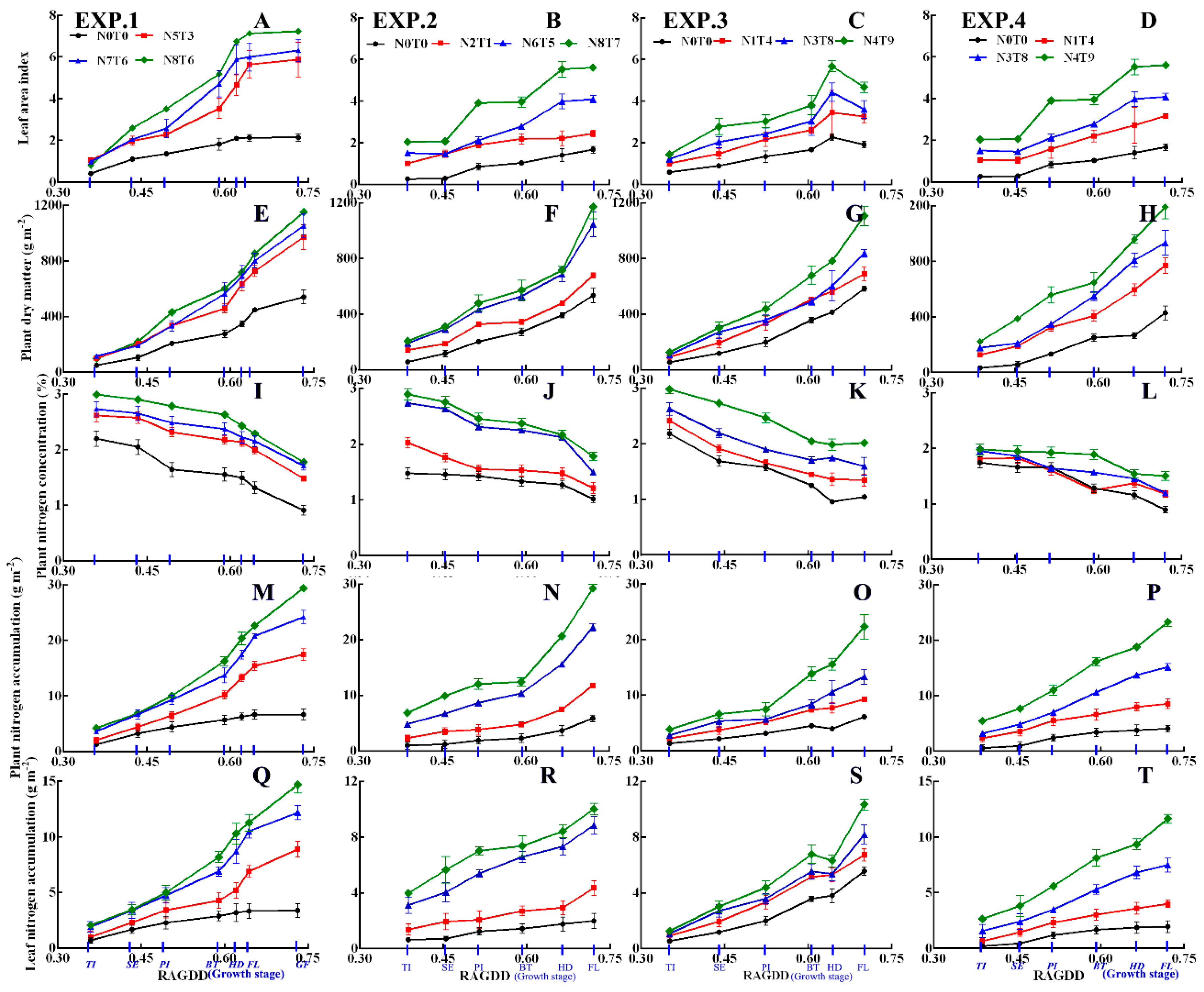
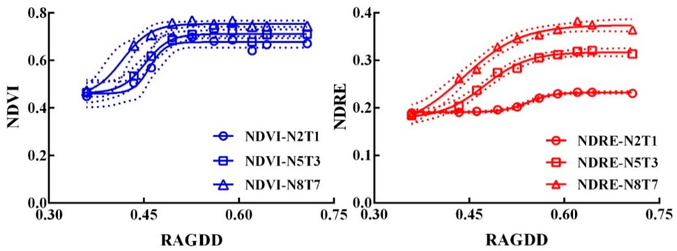
3.1. Dynamic Changes in Agronomic Parameters and Spectral Indexes before Flowering

The dynamic changes in rice agronomic parameters (LAI, PDM, and PNA) in relation to N nutrition were examined in Exp. 1–4 (Figure 2). Similar dynamic characteristics were observed between varieties under different N rates. The results showed that LAI first increased then remained stable (Figure 2A–D). During booting, LAI continued to increase, with the biggest growth rate appearing at the panicle initiation stage. After entering the booting stage, LAI stabilized and remained essentially unchanged thereafter. PDM increased at an invariable rate from tillering to flowering (Figure 2E–H), while PNA was consistent with LNA, continually increasing until flowering (Figure 2M–T). PNC differed slightly from the other N indicators, decreasing up until flowering at an increasing rate (Figure 2I–L).

As shown in Figure 3A–H, NDVI and NDRE increased slowly before stem elongation followed by a rapid rise till booting then a slow increase or static period. This was similar to the changes in LAI. Changes in the RVI and RERVI were similar to those of PDM, PNA, and LNA (Figure 3I–P); however, growth rates differed. The growth rate of PDM and PNA accelerated at the end of the stem elongation stage, while RVI remained relatively stable. PNC showed an opposite trend to all spectral indexes and consistency was also poor. All vegetation indexes showed different values under different N gradients. The red-edge-based vegetation indexes NDRE and RERVI showed higher distinction under different N fertilizer rates, while NDVI showed slight overlap between fertilizer rates. Compared with NDRE, RERVI showed a smaller range before flowering, making it hard to distinguish between growth stages and, therefore, less useful. In each single test, NDRE errors and fluctuations were smaller than those of NDVI, making it more stable. Moreover, ranges of all agronomic parameters were also small, suggesting that the environmental effect on NDVI was much bigger than the effect on NDRE.

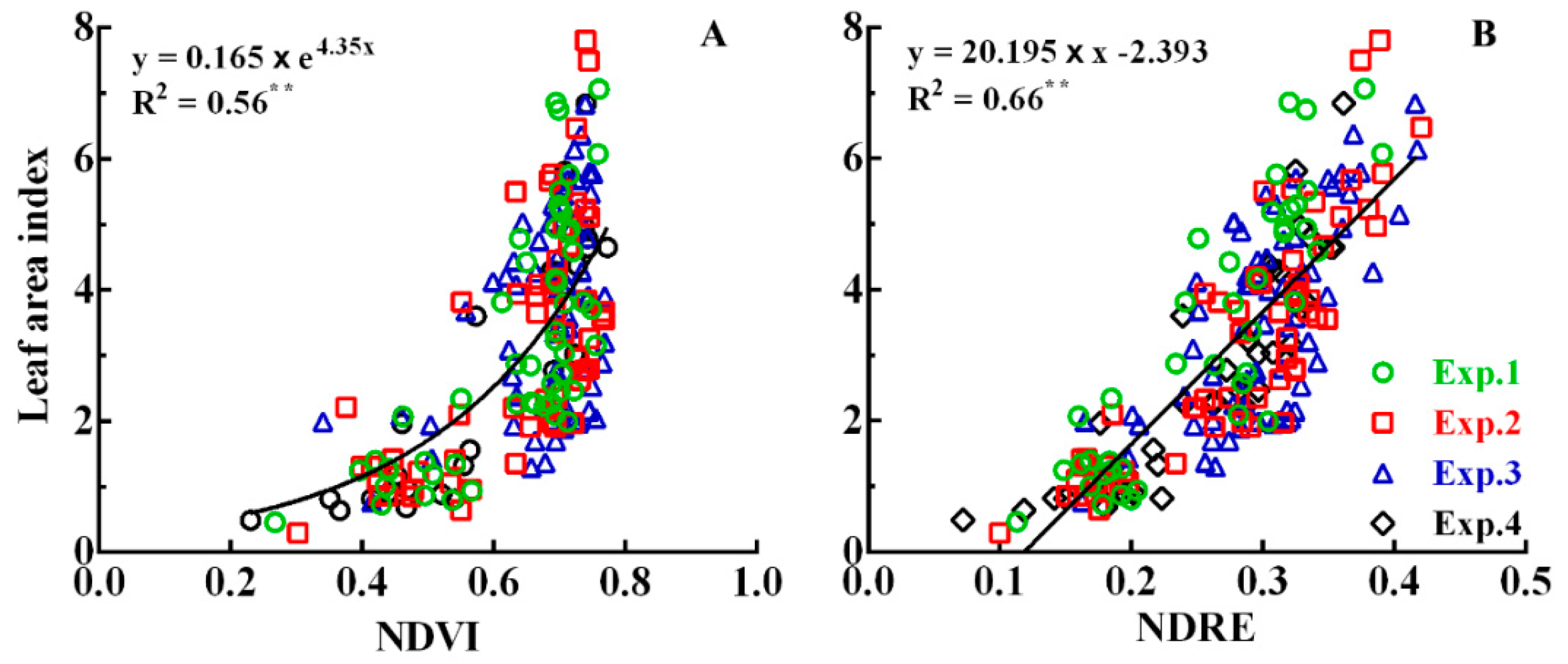
3.2. Relationship between the Spectral Indexes and Agronomic Parameters

Using the results of Exp. 1–4 (

Table 4. Coefficients of determination (R²) of the correlations between vegetation indexes at different stages and the agronomic parameters.

Agronomic Parameter	Spectral Index	Mid-Tillering				Stem Elongation				Panicle Initiation				Booting				Pre-Flowering
		Exp. 1	Exp. 2	Exp. 3	Exp. 4	Exp. 1	Exp. 2	Exp. 3	Exp. 4	Exp. 1	Exp. 2	Exp. 3	Exp. 4	Exp. 1	Exp. 2	Exp. 3	Exp. 4	Exp. 1	Exp. 2	Exp. 3	Exp. 4
LAI	NDRE	0.37	0.70	0.67	0.70	0.51	0.72	0.69	0.71	0.65	0.67	0.77	0.75	0.70	0.75	0.83	0.79	0.67	0.64	0.74	0.78
	NDVI	0.21	0.54	0.50	0.56	0.48	0.69	0.64	0.65	0.58	0.69	0.74	0.64	0.67	0.66	0.74	0.68	0.44	0.66	0.63	0.69
	RERVI	0.37	0.69	0.66	0.70	0.57	0.71	0.71	0.72	0.66	0.70	0.80	0.77	0.71	0.77	0.85	0.81	0.76	0.61	0.78	0.81
	RVI	0.15	0.50	0.43	0.44	0.46	0.70	0.62	0.58	0.63	0.74	0.78	0.66	0.66	0.74	0.77	0.67	0.61	0.57	0.67	0.70
PNC	NDRE	0.49	0.55	0.46	0.13	0.31	0.74	0.46	0.19	0.27	0.70	0.52	0.10	0.34	0.77	0.60	0.37	<0.01	0.26	0.28	0.59
	NDVI	0.30	0.35	0.29	0.07	0.21	0.63	0.39	0.23	0.25	0.58	0.46	0.16	0.32	0.57	0.49	0.35	<0.01	0.20	0.23	0.53
	RERVI	0.50	0.57	0.47	0.14	0.19	0.74	0.40	0.16	0.23	0.73	0.55	0.17	0.43	0.76	0.62	0.39	<0.01	0.24	0.27	0.58
	RVI	0.21	0.33	0.26	0.10	0.31	0.71	0.42	0.11	0.32	0.62	0.48	0.10	0.35	0.66	0.56	0.39	0.01	0.16	0.22	0.51
PNA	NDRE	0.52	0.65	0.66	0.59	0.56	0.64	0.68	0.71	0.58	0.60	0.70	0.70	0.65	0.49	0.67	0.74	0.63	0.51	0.67	0.76
	NDVI	0.33	0.55	0.53	0.53	0.48	0.70	0.63	0.59	0.56	0.54	0.64	0.64	0.61	0.53	0.63	0.60	0.40	0.56	0.56	0.62
	RERVI	0.52	0.62	0.68	0.70	0.59	0.62	0.68	0.72	0.63	0.62	0.73	0.72	0.77	0.51	0.72	0.77	0.74	0.50	0.72	0.79
	RVI	0.26	0.54	0.54	0.63	0.55	0.63	0.64	0.60	0.61	0.58	0.69	0.69	0.72	0.67	0.77	0.72	0.73	0.51	0.69	0.70
LNA	NDRE	0.53	0.67	0.71	0.72	0.64	0.75	0.75	0.71	0.62	0.43	0.62	0.74	0.70	0.69	0.74	0.64	0.63	0.61	0.72	0.79
	NDVI	0.34	0.47	0.51	0.57	0.54	0.72	0.70	0.69	0.55	0.41	0.56	0.64	0.62	0.62	0.65	0.55	0.60	0.64	0.67	0.65
	RERVI	0.52	0.67	0.71	0.73	0.61	0.75	0.74	0.70	0.53	0.46	0.60	0.71	0.63	0.70	0.74	0.66	0.63	0.58	0.71	0.78
	RVI	0.28	0.46	0.49	0.57	0.57	0.74	0.69	0.62	0.51	0.46	0.57	0.62	0.64	0.74	0.75	0.64	0.40	0.55	0.54	0.59

Notes: LAI: leaf area index, PNC: plant nitrogen concentration, PNA: plant nitrogen accumulation, LNA: leaf nitrogen accumulation, NDVI: normalized difference vegetation index, NDRE: normalized difference red edge, RERVI: red-edge ratio vegetation index, RVI: ratio vegetation index. The bold word means higher R² value among four experiments.

), the relationships between each vegetation index and agronomic parameter were also determined, revealing differing results. The relationships between the spectral indexes and LAI and leaf N accumulation were strongest, while those with N concentration were lowest. Moreover, all correlations were low at the tillering stage, increasing with growth until reaching a maximum at stage. During the entire pre-flowering period, the R² of the red-edge band-based indexes were higher than bidirectional reflectance simulation of the red-band-based vegetation indexes. Using the NDRE and NDVI findings in Exp. 1–4, NDVI (Figure 4A) saturation and an intermittent phenomenon were obvious, while the NDRE (Figure 4B) data were more clearly distributed and had a better relationship with LAI. This is also consistent with results in other crops [43]. The relationships between red-edge band-based vegetation indexes and agronomic parameters were, therefore, better than those indexes based on the red band.

We also compared the relationships between agronomic parameters and final yield during the main growth period (

Table 5. Coefficients of determination (R²) of the correlations between the agronomic parameters at different stages and yield.

Growing stage	LAI	PNC	PNA	LNA
Tillering	0.82	0.16	0.73	0.76
Stem elongation	0.72	0.23	0.70	0.67
Panicle initiation	0.73	0.09	0.56	0.74
Booting	0.76	0.42	0.75	0.65

Notes: LAI: leaf area index, PNC: plant nitrogen concentration, PNA: plant nitrogen accumulation, LNA: leaf nitrogen accumulation.

). As pointed out previously, the relationship between agronomic parameters and yield differs at different growth stages [44,45]. This study yielded similar results. The relationship between LAI or N accumulation and yield was best at certain growth stages. Moreover, LAI had the highest coefficient and was more stable than N accumulation, highlighting its potential use in yield predictions.

As mentioned earlier, there were differences in the ranges of NDRE and RERVI before flowering. Stability and distinction between the N gradients of NDRE were better than those of RERVI (Figure 3). Moreover, the dynamic changes in LAI and NDRE were the most consistent (Figure 2 and Figure 3). These results suggest that NDRE can be used to effectively reflect the growth status of rice under different N treatments, and in different eco-sites and different varieties, highlighting its potential use in growth diagnosis and dynamic model construction.

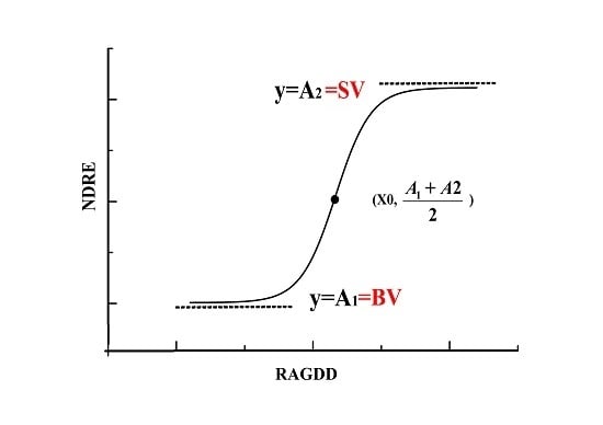
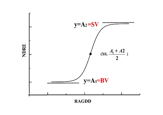
3.3. Construction of a Dynamic Model of NDRE

In this study, NDRE values were stable at first before showing a period of rapid growth throughout the entire pre-flowering stage, followed by a second stable, consistent with sigmoid-curve variation (Figure 5). Therefore, we chose a sigmoid curve to construct the dynamic change model of NDRE (Equation (4)).

$$y=\frac{A_1-A_2}{1+e^{(x-x_0)/dx}}+A_2,$$

(4)

where x represents the time-variable RAGDD, y is the spectral index NDRE value, A₁ is the previous platform value corresponding to the baseline value (BV) in each treatment, A₂ is the medium platform value corresponding to processing of the saturation value (SV), and $x_0$ is the midpoint of the sigmoid curve, that is, the point at which the model reaches inflection, indicating the different stages of dynamic change (Figure 5). Before $x_0$, rice is considered to be in the rapid growth stage, while, after $x_0$, the growth rate decreases and the population reaches a peak. Moreover, when $x=x_0$, $x=\frac{A_1+A_2}{2}$, the growth rate of the model is at its highest. Finally, $dx$ represents the time constant of the model.

At early and mid-tillering stages, resource requirements including fertilizer and water were relatively small, resulting in a small growing base. Moreover, vegetation coverage was also small, causing the canopy spectra to contain a lot of water and soil background information. As a result, the NDRE values were low and fluctuated around BV. In the mid-stage of growth, particularly early stem elongation, the growth rate increased rapidly, leading to a rapid growth period. After this, in the late stem elongation and booting stages, growth gradually reached a peak, and spectral index growth slowed until flowering.

Results of low (N2T1, 60 + 40 kg·ha⁻¹), medium (N5T3, 120 + 80 kg·ha⁻¹), and high (N8T7, 240 + 160 kg·ha⁻¹) N fertilizer averages are shown in Figure 6. At early growth stages, the differences in NDRE were not significant; however, SV values differed during mid-growth stages. The SV of N2T1 was low at approximately 0.23, while the values of N5T3 and N8T7 were 0.29 and 0.38. Meanwhile, NDVI arrived at its threshold earlier than NDRE as shown in Figure 6, and it was hard to distinguish between N2T1, N5T3, and N8T7 treatments.

The model parameters were mainly obtained by fitting the measured values obtained at a high frequency testing, that is, under Exp. 1 and 3. In addition, BV and SV parameters were also estimated from NDRE values obtained at corresponding growth stages. For example, in the stem elongation to booting stages, NDRE entered the mid-stage of growth in the SV period. At this time, regardless of measurement errors, the measured NDRE values were approximately equal to the SV value. The SVs of Exp. 2 and Exp. 4 were subsequently obtained using this method. At the latest, SV values are determined at the early date.

3.4. Testing of Each Vegetation Index-Based Dynamic Model and Parameter Analysis

3.4.1. Verification of Model Construction Correctness

To confirm the accuracy of the dynamic models, they were fitted using each experiment and N treatment (

Table 6. Summary of fitting analysis of the NDRE dynamic model under each treatment.

NDRE Exp. 1				NDRE Exp. 3				NDVI Exp. 1				NDVI Exp. 3
Treatments	R2	RRMSE (%)	p-Value of Residual’s Normality	Treatments	R2	RRMSE (%)	p-Value of Residual’s Normality	Treatments	R2	RRMSE (%)	p-Value of Residual’s Normality	Treatments	R2	RRMSE (%)	p-Value of Residual’s Normality
N0T0	0.94	4.83	0.89	N0T0	0.94	2.43	0.9	N0T0	0.82	14.5	0.64	N0T0	0.87	21.0	0.72
N5T0	0.94	2.52	0.65	N2T0	0.9	1.55	0.69	N5T0	0.9	13.0	0.96	N2T0	-	-	-
N5T3	0.97	2.26	0.62	N2T1	0.93	2.17	0.79	N5T3	0.92	13.5	0.81	N2T1	0.89	19.0	0.9
N7T0	0.94	2.35	0.39	N6T0	0.95	1.07	0.49	N7T0	0.91	15.0	0.89	N6T0	0.91	17.0	0.84
N7T6	0.94	3.68	0.74	N6T5	0.96	1.9	0.51	N7T6	0.93	17.0	0.9	N6T5	0.92	16.0	0.97
N8T0	0.96	2.34	0.5	N8T0	0.9	1.93	0.29	N8T0	0.94	11.0	0.95	N8T0	0.83	15.0	0.73
N8T7	0.97	2.44	0.56	N8T7	0.91	2.59	0.44	N8T7	0.95	7.5	0.79	N8T7	0.9	16.0	0.81

Notes: RRMSE: relative root-mean-square error; “N0T0, N5T0, N5T3, N6T0, N7T0, N7T6, N8T0, and N8T7” represent different basal and topdressing N fertilizer rates (0 + 0, 120 + 0, 120 + 80, 150 + 0, 180 + 0, 180 + 120, 240 + 0, and 2400 + 160 kg∙ha⁻¹, respectively). The normality test was conducted using the Shapiro–Wilk method at 0.05 significance. Reason for the fitting’s failure was due to mutual dependency existence between parameters.

). The results of model fitting based on NDRE showed that the R² values of different N gradients were greater than 0.9, while the values of RRMSE were less than 5%, suggesting that model values showed very small differences compared to the measured values, also indicating that the modeling effect of the different gradients was good. The normal distribution test of standard residuals under each treatment model showed that the probability of normal distribution was greater than 0.05, revealing that the standard residuals of each treatment were within normal distribution and that the model errors were random and generated by the model itself. Model fitting based on NDVI resulted in a high R² (0.87–0.96); however, the range of RRMSE was 7.5–21% higher than that of NDRE. Overall, these findings suggest that the model was applicable under different N levels, with different varieties, in different eco-sites, and in different years, confirming the accuracy of the model.

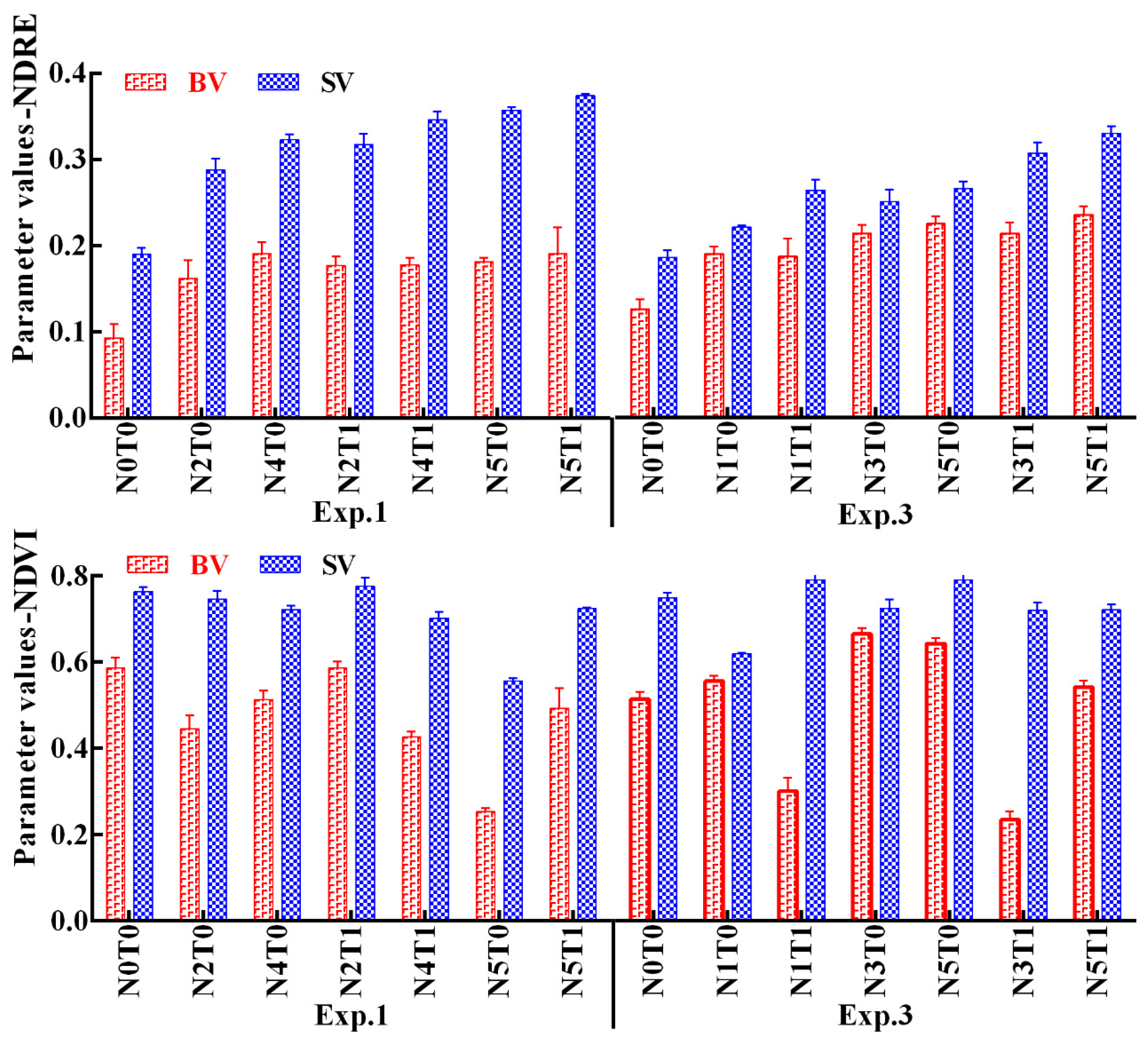
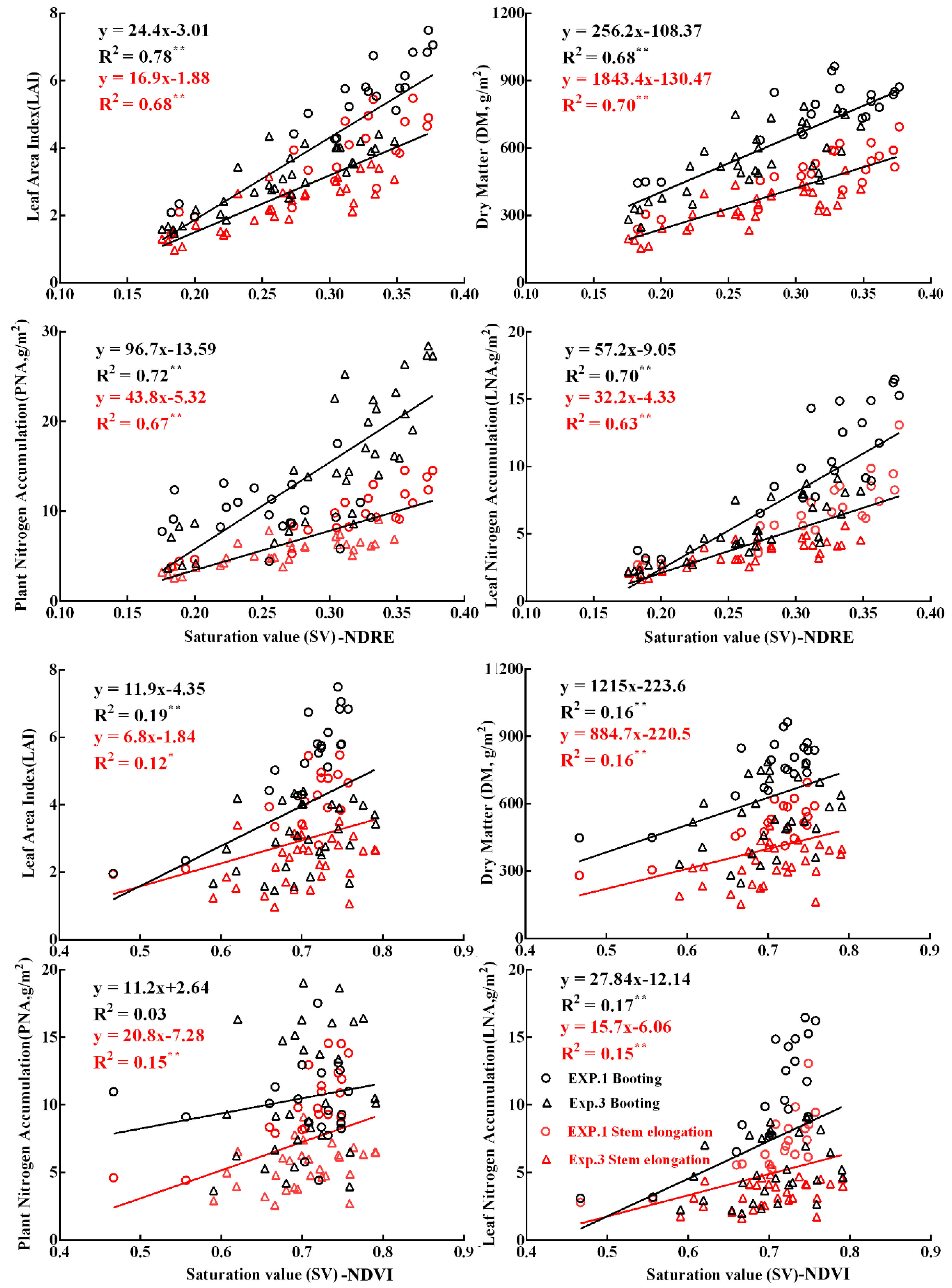
3.4.2. Changes in BV and SV under Different Treatments and Their Relationship with Agronomic Parameters

The NDRE values changed little at early stages of growth, fluctuating around the BV value. The BV under each treatment was less than 0.25 and there were no differences between treatments (Figure 7, NDRE), while BV and SV estimated using NDVI showed no obvious regularity. SV calculated using NDRE increased with increasing N fertilizer rates, and the trends between treatments were consistent. The differences with topdressing under the same basal fertilizer also differed, and the SV of T0 decreased by 15–25%. Moreover, a 10% increase in SV was observed between N0T0 and N5T0, N5T0 and N7T0, and N7T0 and N8T0. The differences between N application and topdressing levels also differed, suggesting that SV has obvious potential in growth status analysis in rice.

The relationship between SV and agronomic parameters was subsequently examined using the data from Exp. 1 and Exp. 3 (Figure 8). The relationships between SV and LAI, PDM, PNA, and LNA were good at both stem elongation (fourth leaf from the top stage) and booting stage (second leaf from the top stage). For NDRE, the R² of each of these relationships was more than 0.6. At stem elongation, there were slight differences but essentially similar correlations between SV and LAI, PDM, PNA, and LNA. Correlations at booting stage were better than those at stem elongation. Overall, LAI had the best relationship with SV. However, with NDVI, poor correlation was observed between all parameters.

Variation in the critical point $x_0$ under each treatment was also examined. As shown in

Table 7. Distribution of the critical point of dynamic change under a single time series.

Experiment	Exp. 1
Treatment	N0T0	N5T0	N7T0	N5T3	N8T0	N7T6	N8T3
(kg∙ha−1)	0	120	180	200	240	300	320
RAGDD	0.366	0.374	0.351	0.357	0.303	0.345	0.314
	Exp. 3
Treatment	N0T0	N2T0	N2T1	N6T0	N6T2	N8T0	N8T3
(kg∙ha−1)	0	60	100	150	200	240	320
RAGDD	0.516	0.55	0.524	0.559	0.538	0.494	0.542

Notes: “N8T0, N8T3, N7T6, N7T0, N5T3, N0T0, N5T0, N2T1, N6T2, N2T0, and N6T0” represent different basal and topdressing N fertilizer rates (240 + 0, 240 + 80, 180 + 120, 180 + 0, 120 + 80, 0 + 0, 120 + 0, 60 + 40, 150 + 50, 60 + 0, and 150 + 0 kg∙ha⁻¹, respectively).

, the model reached a critical point of dynamic change earlier in Exp. 1 than Exp. 3. This was especially true under identical N fertilizer treatments, namely, 0, 200, 240, and 320 kg·N·ha⁻¹ N fertilizer topdressing. Moreover, the earliest critical point was observed under N8T0 (240 kg·N·ha⁻¹) treatment in both experiments (Exp. 1 and Exp. 3). Meanwhile, 100–200 kg·N·ha⁻¹ plots showed the highest average RAGDD values.

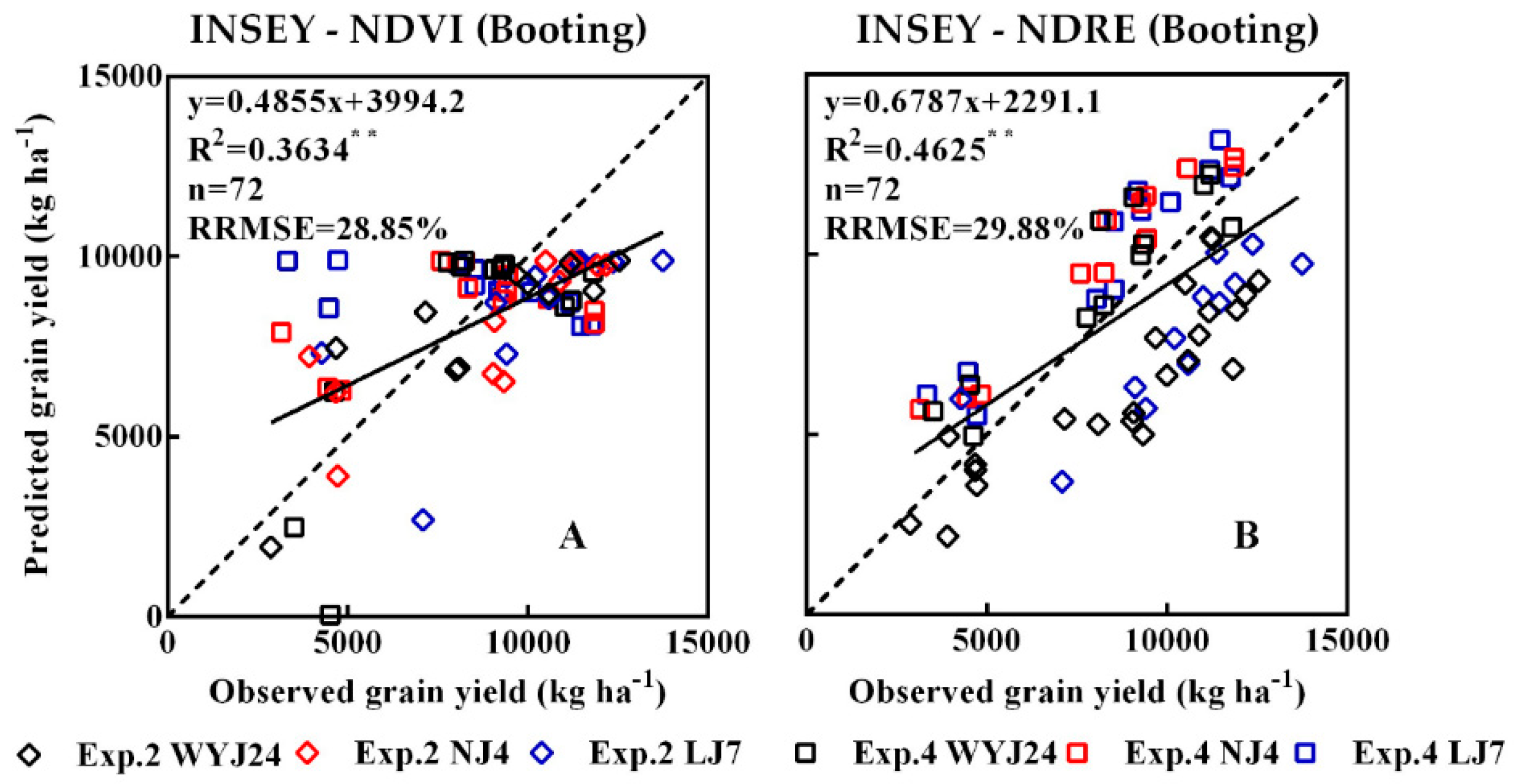
3.5. Prediction Algorithm for Rice Grain Yield

The relationship between BV, SV, and $x_0$ with grain yield was also studied (Figure 9). The results showed a poor relationship between BV and yield (Figure 9A,E), while $x_0$ value was negatively correlated with yield, and, although the correlation was poor, differences were observed among cultivars (Figure 9B,F). There were no differences in SV between experiments, suggesting that SV showed the similar correlations with yield between different years, eco-sites, and varieties (Figure 9C). Meanwhile, the NDVI-based SV was poorly correlated with grain yield.

The quantitative relationship between SV and grain yield was developed (Figure 10) using the data from Exp. 1 and Exp. 3. As shown in Figure 10, grain yield was forecast using linear regression analysis based on the SV values. Grain yield was evenly distributed from 6000 to 13000 kg·ha⁻¹ and the model was good. The slope of the linear model was 36081 kg·ha⁻¹, suggesting that with every 0.1 increase in SV, yield increased by 3608.1 kg·ha⁻¹.

The data from Exp. 2 and Exp. 4 were subsequently used to test the accuracy of the SV-based yield prediction model (Figure 11). As shown, in Figure 11A, SV was obtained from the fitted sigmoid curve model, while, in Figure 11B, values were estimated using measured NDRE values from the stem elongation to booting stages. Both methods gave good prediction results. The predicted yields in both study years showed no obvious abnormalities compared with the observed yield, and the overall prediction error was approximately 20%. These findings suggest that the model is applicable in different varieties and different rice planting regions under different SV acquisition methods.

We also used the same data from the same growth stages to estimate yield using INSEY (Figure 12) [46]. Of all stages, the best correlation was obtained in booting stage. As shown in Figure 12A, the R² of the INSEY-NDVI model was low with poor accuracy. Meanwhile, the INSEY-NDRE model had 70% prediction accuracy, but this was still less accurate than the SV-based yield prediction algorithm by about 10% (Figure 12B).

4. Discussion

4.1. Spectral Indexes for Rice Growth Diagnosis

NDVI is the most widely used spectral index. However, because of the characteristics of red light in NDVI itself [47,48], saturation occurs when the population or coverage reaches a certain level, thereby affecting the monitoring effect [41]. Muñoz-Huerta et al. revealed a positive linear relationship between RVI and N uptake in winter wheat, as well as insensitivity to growth stage and crop variety. In addition, RVI was previously used to estimate N status in over-fertilized fields [49]. It was also suggested that the red-edge-based vegetation indexes (RVI, NDRE) perform well in estimating NNI and plant N accumulation [37]. In this study, serious overlap and a cross between obtained values and the error ranges of different gradients in spectral indexes containing red bands was observed after stem elongation, preventing clarification of the differences between N gradients. Studies showed that the absorption of chlorophyll on the red-edge waveband is weaker than that of red light, with the red-edge region having stronger transmission ability with the crop canopy and leaf [25]. Use of red-edge rather than red-light bands can, therefore, reduce the saturation phenomenon, enhancing monitoring and diagnosis of crop N nutrition.

In this study, NDVI did not distinguish between different N treatments during mid-growth and late growth stages, similar to the findings of Liu et al. [41]. It was also previously revealed that, at an early growth stage (before stem elongation), NDVI resulted in a better relationship with rice grain yield; however, on approaching maturity, NDRE performed better [50]. Red-edge-based NDRE reflects this phenomenon via differences in saturation values. Our results suggest that the shortcoming of NDVI is that saturation at an early stage leads to no differences in SV with varying N rates. Yumiko et al. also reported that NDVI reached saturation earlier than NDRE under different N rates [50]. NDVI can, therefore, be used to determine low-land rice at early growth stages, but is less useful at mid-growth to late growth stages. Moreover, using vegetation indexes with the red-light band, correlations with agronomic parameters were poor, while the red-edge band-based indexes (NDRE and RERVI) showed a linear relationship with agronomic parameters, allowing differences between N fertilizer levels to be distinguished. However, changes in RERVI throughout the entire growth period were small, thereby preventing effective analysis between different stages. In the same plot, NDRE showed lower variability than RERVI. These findings suggest that NDRE can be used to reflect the growth status of different treatments, making it a suitable index for diagnosis of rice growth.

4.2. The Dynamic Model and Parameters of Rice Spectral Indexes

The results of this study suggest that NDRE conforms to a sigmoid curve. In early stages, NDRE fluctuated around background BV values at a low level. However, values began to rise rapidly after tillering. The critical point ($x_0$) of the dynamic model was then reached on entering stem elongation. Meanwhile, at flowering stage, the dynamic model became stable again and approached the feature platform SV.

Previous monitoring methods such as the saturation index (SI) method and NNI are based mainly on data collected at each growth stage [8]. These methods mostly lack biophysical mechanisms, often fail to obtain indicators, and consist of a complex calculation method [25]. Moreover, deviations in identification of growth stages, environmental factors, time selection, and so on have a significant impact on these single tests. Furthermore, single measured values are treated as a reflection of an entire stage in the calculations, resulting in greater deviation from the actual values [51].

In this paper, the parameters in the model have practical biological meaning. The range of $x_0$ reflects growth and development of rice at early stages. The findings also suggest that higher $x_0$ values occur under abnormally high temperatures in early stages compared with normal growing conditions. The $x_0$ value can be used as an indicator of the growth environment during early stages of growth; however, the poor correlation between $x_0$ and grain yield prevented quantification of yield predictions.

BV was also able to reflect growth status at early stages. However, when rice coverage was less than 50%, including the depth of the water layer, turbidity, soil background color, and so on, there was an impact on the spectral reflectance test [52,53]. In this study, BV values were low under all treatments, and no obvious differences between gradients were observed. Meanwhile, BV did not distinguish between differences in basal fertilizers levels in early stages of growth, suggesting that water and soil background information under low coverage conditions during this period obscure growth information contained in the spectral data. BV is, therefore, not applicable for direct monitoring and diagnosis of rice growth, although differences in LAI and other agronomic parameters were obvious. In the future, we aim to increase accuracy by adding variables such as coverage, soil, and water to improve the signal-to-noise ratio.

In the middle of the growing season, SV values overcame the above problems in $x_0$ and BV. SV values differed between different rice populations under different treatments and in different groups, and there was a good linear relationship with agronomic parameters such as LAI and aboveground N accumulation. SV values could be obtained not only from the fitted model, but also from measured values. Overall, the accuracy and availability of the model were high, confirming applicability for monitoring and diagnosis.

The dynamic model was successfully used to determine growth status using different rice varieties, in different eco-sites, and under different N rates before flowering with 90% variation. Bonfil et al. also reported similar dynamic changes in wheat in 2016 [52]. Moreover, our dynamic model also determined the growth status of paddy rice using RapidScan CS-45 at different grain yield levels. Of course, it can also be used to predict yield before flowering without any specific calibration. It should also be used on non-rainy days, since water droplets on the blade affect monitoring. In the future, the growth status after flowering stage will be examined further, and additional vegetation indexes will be used in developing a dynamic model.

4.3. SV-Based Yield Prediction Algorithm

In previous studies, spectral indexes were used to predict yield in crops such as wheat [54] and sugarcane [55] with good results. Bonfil used RapidScan CS-45 to monitor the dynamic changes in wheat, revealing a good linear relationship between NDRE and wheat yield in different varieties [54]. In this study, the dynamic pattern of NDRE at pre-flowering stages was consistent, and predicted yield was achieved under optimal growing conditions other than limited N fertilizer. Kanke et al. also revealed that vegetation indexes containing the red-edge band had a better linear relationship with agronomic parameters and yield at main growth stages in rice [55]. A linear model of yield prediction using different vegetation indexes as input variables was also established, within which NDRE and RERVI gave best correlations, with R² values greater than 0.8. However, the prediction equation was predicted using data from a single growth stage, and the parameters differed between stages, making it of no use between stages or deviations [56]. Similarly, Cowley et al. established an NDVI-based model for forecasting of rapeseed yield [57], while Liu et al. proved the dynamic model could be continuously used to monitor N nutrition status in a single growing season [41]. However, it could only be used when GDD was between 210 and 320 °C.

Thus, the problem of low prediction accuracy resulting from NDVI saturation when using traditional algorithms in rice under high yield conditions remains unsolved. In this study, SV showed a good linear relationship with agronomic parameters and yield. Moreover, SV values were the feature platform of each treatment, eliminating deviations between tests and different environments, thereby increasing applicability of the model, improving stability of the algorithm, and widening the available time range. In addition, SV values could be obtained not only from the fitted model, but also from measured values. Moreover, measurement and processing are relatively simple and do not require normalization or other transformations to maintain accuracy, simplifying our method compared with other algorithms [58].

Satellite remote sensing (RS) data were extensively applied to a wide range of research problems and practical applications, including yield predictions [59]. Zhu et al. used Moderate Resolution Imaging Spectroradiometer Enhanced Vegetation Index (MODIS EVI) time-series data to predict yield in winter wheat, revealing a high R² (0.70) and low RMSE (343.34 kg∙hm⁻²) [60]. Furthermore, Fletcher reported continuity of multispectral high-resolution optical observations over global terrestrial surfaces using Sentinel 2 [61], providing detailed information within field variability [62]. Our newly developed SV-based yield prediction algorithm must now be tested and applied under different RS platforms, such as unmanned aerial vehicles and Sentinel 2.

4.4. Interval System Errors between Experiments and Uncertainties of the Model

In different experiments, trends in indicators were basically the same, although the ranges of change were quite different, especially in Exp. 1 (2015) and Exp. 3 (2016). This was possibly due to the differences in meteorological conditions in 2015 and 2016 (Figure 13). From June to early July 2016, the temperature was slightly higher than in 2015; thus, growth was relatively fast in early and mid-tillering. However, in late July to August, unusually high temperatures and continuous rain occurred, which is not conducive to rice growth and development, thereby inhibiting growth. As a result, the agronomic parameters, spectral indexes, and other indicators decreased sharply in 2015.

This phenomenon was also reflected in another way. In both years, $x_0$ values remained relatively concentrated at the end of the tillering stage; however, there were differences between N rates. Moreover, the critical point shifted in 2016 compared to 2015. The average daily temperature was higher than 33 °C at the end of tillering and early stem elongation stage in Exp. 3, 2016. The optimum temperature of paddy rice at tillering is 25~30 °C, while the maximum temperature is 32 °C [42] (Figure 13). As a result, these high temperatures caused an abnormal increase in the RAGDD time variable, even though growth was inhibited and $x_0$ increased.

Model uncertainty received considerable attention in recent studies [63]. There is growing pressure on crop field production to conform to quality standards, which require evaluation and expression of the uncertainty of measurement results [64]. It is, therefore, important to determine the degree of uncertainty associated with a model and its application in predicting crop N status and yield. In this study, the dynamic model was developed using a large database, diverse eco-sites, different rice varieties, and differing N rates; however, errors were revealed when the model output was compared with observations. Moreover, it is difficult to evaluate uncertainty in practice. For example, the uncertainty of certain components is often unknown in crop field experiments, such as those associated with environmental effects or different sensors. During the 2015–2017 growing season, the sensors were calibrated each year to avoid errors; however, additional field experiments are needed to expand the database and therefore improve the robustness of our dynamic model.

5. Conclusions

We used the active spectrometer RapidScan CS-45 to determine the dynamic changes in different spectral indexes and agronomic parameters in rice. The results suggest that NDRE is more stable than other indexes, with the distinctions between different treatment gradients most obvious. NDRE also had the best relationship with agronomic parameters. The dynamic changes in NDRE and LAI were similar, and followed a “slow–fast–slow” trend during the pre-flowering period.

A sigmoid curve was used in NDRE dynamic model construction, with high accuracy and an R² of 0.9 and RRMSE of 5%. The model contained critical point $x_0$, background value BV, and feature platform value SV parameters. The relationships with yield showed that each of these parameters was correlated with yield, although SV was better than the other two parameters. SV showed a good linear relationship with in-season potential grain. Based on these findings, we constructed a yield prediction model. With every 0.1 increase in SV, grain yield increased by 3608.1 kg·ha⁻¹. The overall prediction accuracy of the model was greater than 80%. It can be used at stem elongation and booting, improving timeliness compared with existing forecasting algorithms. Our model is, therefore, useful for rice production management, purchasing and storage preparation, rice spot price trend forecasts, and food policy decision-making.

References

1. Lundström, C.; Lindblom, J.; Hansen, J.W.; Thornton, P.K.; Berentsen, P.B.M. Considering farmers’ situated knowledge of using agricultural decision support systems (AgriDSS) to Foster farming practices: The case of CropSAT. Agric. Syst. 2018, 159, 9–20. [Google Scholar] [CrossRef]
2. Zhang, H.; Zhang, J.; Gong, J.; Yong, C.; Min, I.; Hui, G.; Dai, Q.; Huo, Z.; Ke, X.; Wei, H. The productive advantages and formation mechanisms of “Indica Rice to Japonica Rice”. Sci. Agric. Sinica 2013, 46, 686–704. [Google Scholar]
3. He, J.; Xiao, H.; Huang, X.; Zhou, Q.; Hu, D. Effects of real-time and site-specific nitrogen management on rice yield and nitrogen use efficiency. Southwest China J. Agric. Sci. 2010, 23, 1132–1136. [Google Scholar]
4. Diacono, M.; Rubino, P.; Montemurro, F. Precision nitrogen management of wheat. A review. Agron. Sustain. Dev. 2013, 33, 219–241. [Google Scholar] [CrossRef]
5. Peng, S.; Buresh, R.J.; Huang, J.; Zhong, X.; Zou, Y.; Yang, J.; Wang, G.; Liu, Y.; Hu, R.; Tang, Q. Improving nitrogen fertilization in rice by Site-Specific N Management. Agron. Sustain. Dev. 2010, 30, 649–656. [Google Scholar] [CrossRef]
6. Huang, J.; He, F.; Cui, K.; Buresh, R.J.; Xu, B.; Gong, W.; Peng, S. Determination of optimal nitrogen rate for rice varieties using a chlorophyll meter. Field Crops Res. 2008, 105, 70–80. [Google Scholar] [CrossRef]
7. Peng, S.; Garcia, F.V.; Laza, R.C.; Sanico, A.L.; Visperas, R.M.; Cassman, K.G. Increased N-use efficiency using a chlorophyll meter on high-yielding irrigated rice. Field Crops Res. 1996, 47, 243–252. [Google Scholar] [CrossRef]
8. Bijay-Singh; Varinderpal-Singh; Yadvinder-Singh; Thind, H.S.; Kumar, A.; Gupta, R.K.; Kaul, A.; Vashistha, M. Fixed-time adjustable dose site-specific fertilizer nitrogen management in transplanted irrigated rice (Oryza sativa L.) in South Asia. Field Crops Res. 2012, 126, 63–69. [Google Scholar] [CrossRef]
9. Yi, Q.; Zhao, S.; Zhang, X.; Yang, L.; Xiong, G.; He, P. Yield and nitrogen use efficiency as influenced by real time and site specific nitrogen management in two rice cultivars. Plant Nutr. Fertil. Sci. 2012, 18, 777–785. [Google Scholar]
10. Fan, L.; Peng, X.; Liu, Y.; Song, T. Study on the site-specific nitrogen management of rice in cold area of northeastern China. Sci. Agric. Sinica 2005, 38, 1761–1766. [Google Scholar]
11. Justes, E.; Mary, B.; Meynard, J.M.; Machet, J.M.; Thelierhuche, L. Determination of a critical nitrogen dilution curve for winter wheat crops. Ann. Bot. 1994, 74, 397–407. [Google Scholar] [CrossRef]
12. Greenwood, D.J.; Neeteson, J.J.; Draycott, A. Quantitative relationships for the dependence of growth rate of arable crops on their nitrogen content, dry weight and aerial environment. Plant Soil 1986, 91, 281–301. [Google Scholar] [CrossRef]
13. Lemaire, G.; Jeuffroy, M.H.; Gastal, F. Diagnosis tool for plant and crop N status in vegetative stage: Theory and practices for crop N management. Eur. J. Agron. 2008, 28, 614–624. [Google Scholar] [CrossRef]
14. Ata-Ul-Karim, S.T.; Liu, X.; Lu, Z.; Yuan, Z.; Zhu, Y.; Cao, W. In-season estimation of rice grain yield using critical nitrogen dilution curve. Field Crops Res. 2016, 195, 1–8. [Google Scholar] [CrossRef]
15. Xia, T.; Miao, Y.; Wu, D.; Shao, H.; Khosla, R.; Mi, G. Active optical sensing of spring maize for in-season diagnosis of nitrogen status based on nitrogen nutrition index. Remote Sens. 2016, 8, 605. [Google Scholar] [CrossRef]
16. Zhao, B.; Liu, Z.; Ata-Ul-Karim, S.T.; Xiao, J.; Liu, Z.; Qi, A.; Ning, D.; Nan, J.; Duan, A. Rapid and nondestructive estimation of the nitrogen nutrition index in winter barley using chlorophyll measurements. Field Crops Res. 2016, 185, 59–68. [Google Scholar] [CrossRef]
17. Ata-Ul-Karim, S.T.; Liu, X.; Lu, Z.; Zheng, H.; Cao, W.; Zhu, Y. Estimation of nitrogen fertilizer requirement for rice crop using critical nitrogen dilution curve. Field Crops Res. 2017, 201, 32–40. [Google Scholar] [CrossRef]
18. Hu, Y.; Yang, J.P.; Lv, Y.M.; He, J.J. SPAD values and nitrogen nutrition index for the evaluation of rice nitrogen status. Plant Prod. Sci. 2014, 17, 81–92. [Google Scholar]
19. Houlès, V.; Guérif, M.; Mary, B. Elaboration of a nitrogen nutrition indicator for winter wheat based on leaf area index and chlorophyll content for making nitrogen recommendations. Eur. J. Agron. 2007, 27, 1–11. [Google Scholar] [CrossRef]
20. Debaeke, P.; Rouet, P.; Justes, E. Relationship between the normalized SPAD index and the nitrogen nutrition index: Application to durum wheat. J. Plant Nutr. 2006, 29, 75–92. [Google Scholar] [CrossRef]
21. Ata-Ul-Karim, S.T.; Zhu, Y.; Liu, X.; Cao, Q.; Tian, Y.; Cao, W. Comparison of different critical nitrogen dilution curves for nitrogen diagnosis in rice. Sci. Rep. 2017, 7, 42679. [Google Scholar] [CrossRef] [PubMed] [Green Version]
22. Bogdan, K.; Andrzej, L.; Andrzej, O.; Marek, K. The effect of tillage system and forecrop on the yield and values of LAI and SPAD indices of spring wheat. Eur. J. Agron. 2010, 33, 43–51. [Google Scholar]
23. Spitkó, T.; Nagy, Z.; Zsubori, T.; Szőke, C.; Berzy, T.; Pintér, J.; Márton, L. Connection between normalized difference vegetation index and yield in maize. Plant Soil Environ. 2016, 62, 293–298. [Google Scholar] [CrossRef] [Green Version]
24. Tubaña, B.S.; Harrell, D.L.; Walker, T.; Teboh, J.; Lofton, J.; Kanke, Y. In-season canopy reflectance-based estimation of rice yield response to nitrogen. Agron. J. 2012, 104, 1604–1611. [Google Scholar] [CrossRef]
25. Liu, K.; Yazhen, L.I.; Huiwen, H.U. Estimating the effect of urease inhibitor on rice yield based on NDVI at key growth stages. Front. Agric. Sci. Eng. 2014, 1, 150–157. [Google Scholar] [CrossRef]
26. Xue, L.; Li, G.; Qin, X.; Yang, L.; Zhang, H. Topdressing nitrogen recommendation for early rice with an active sensor in south China. Precis. Agric. 2014, 15, 95–110. [Google Scholar] [CrossRef]
27. Evert, F.K.V.; Booij, R.; Jukema, J.N.; Berge, H.F.M.T.; Uenk, D.; Meurs, E.J.J.; Geel, W.C.A.V.; Wijnholds, K.H.; Slabbekoorn, J.J. Using crop reflectance to determine sidedress N rate in potato saves N and maintains yield. Eur. J. Agron. 2012, 43, 58–67. [Google Scholar] [CrossRef]
28. Morier, T.; Cambouris, A.N.; Chokmani, K. In-season nitrogen status assessment and yield estimation using hyperspectral vegetation indices in a potato crop. Agron. J. 2015, 107, 1295–1309. [Google Scholar] [CrossRef]
29. Lukina, E.V.; Freeman, K.W.; Wynn, K.J.; Thomason, W.E.; Mullen, R.W.; Stone, M.L.; Solie, J.B.; Klatt, A.R.; Johnson, G.V.; Elliott, R.L. Nitrogen fertization optimization algorithm based on in-season estimates of yield and plant nitrogen uptake. J. Plant Nutr. 2001, 24, 885–898. [Google Scholar] [CrossRef]
30. Raun, W.R.; Solie, J.B.; Johnson, G.V.; Stone, M.L.; Lukina, E.V.; Thomason, W.E.; Schepers, J.S. In-season prediction of potential grain yield in winter wheat using canopy reflectance. Agron. J. 2001, 93, 131–138. [Google Scholar] [CrossRef]
31. Cao, Q.; Miao, Y.; Shen, J.; Yu, W.; Yuan, F.; Cheng, S.; Huang, S.; Wang, H.; Yang, W.; Liu, F. Improving in-season estimation of rice yield potential and responsiveness to topdressing nitrogen application with Crop Circle active crop canopy sensor. Precis. Agric. 2016, 17, 136–154. [Google Scholar] [CrossRef]
32. Shaver, T.M.; Khosla, R.; Westfall, D.G. Evaluation of two ground-based active crop canopy sensors in maize: Growth stage, row spacing, and sensor movement speed. Soil Sci. Soc. Am. J. 2010, 74, 2101–2108. [Google Scholar] [CrossRef]
33. Li, F.; Etc, Y.M. Estimating winter wheat biomass and nitrogen status using an active crop sensor. Intell. Autom. Soft Comput. 2010, 16, 1221–1230. [Google Scholar]
34. Lofton, J.; Tubana, B.S.; Kanke, Y.; Teboh, J.; Viator, H.; Dalen, M. Estimating sugarcane yield potential using an in-season determination of normalized difference vegetative index. Sensors 2012, 12, 7529. [Google Scholar] [CrossRef] [PubMed]
35. Yao, Y.; Miao, Y.; Jiang, R.; Khosla, R.; Gnyp, M.L.; Bareth, G. Evaluating different active crop canopy sensors for estimating rice yield potential. In Proceedings of the Second International Conference on Agro-Geoinformatics, Fairfax, VA, USA, 12–16 August 2013; pp. 538–542. [Google Scholar]
36. Thompson, L.J.; Ferguson, R.B.; Kitchen, N.; Frazen, D.W.; Mamo, M.; Yang, H.; Schepers, J.S. Model and sensor-based recommendation approaches for in-season nitrogen management in corn. Agron. J. 2015, 107, 2020–2030. [Google Scholar] [CrossRef]
37. Cao, Q.; Miao, Y.; Wang, H.; Huang, S.; Cheng, S.; Khosla, R.; Jiang, R. Non-destructive estimation of rice plant nitrogen status with Crop Circle multispectral active canopy sensor. Field Crops Res. 2013, 154, 133–144. [Google Scholar] [CrossRef]
38. Russelle, M.P.; Wilhelm, W.W.; Olson, R.A.; Power, J.F. Growth analysis based on degree days. Crop Sci. 1984, 24, 28–32. [Google Scholar] [CrossRef]
39. Su, L.; Wang, Q.; Bai, Y. An analysis of yearly trends in growing degree days and the relationship between growing degree day values and reference evapotranspiration in Turpan area, China. Theor. Appl. Climatol. 2013, 113, 711–724. [Google Scholar] [CrossRef]
40. Liu, X.; Ferguson, R.B.; Zheng, H.; Cao, Q.; Tian, Y.; Cao, W.; Zhu, Y. Using an active-optical sensor to develop an optimal NDVI dynamic model for high-yield rice Production (Yangtze, China). Sensors 2017, 17, 672. [Google Scholar] [CrossRef]
41. Li, H.; Zhao, C.; Yang, G.; Feng, H. Variations in crop variables within wheat canopies and responses of canopy spectral characteristics and derived vegetation indices to different vertical leaf layers and spikes. Remote Sens. Environ. 2015, 169, 358–374. [Google Scholar] [CrossRef]
42. Kanke, Y.; Raun, W.; Solie, J.; Stone, M.; Taylor, R. Red edge as a potential index for detecting differences in plant nitrogen status in winter wheat. J. Plant Nutr. 2012, 35, 1526–1541. [Google Scholar] [CrossRef]
43. Prasad, B.; Carver, B.F.; Stone, M.L.; Babar, M.A.; Raun, W.R.; Klatt, A.R. Genetic analysis of indirect selection for winter wheat grain yield using spectral reflectance indices. Crop Sci. 2007, 47, 1416–1425. [Google Scholar] [CrossRef]
44. Gutierrez, M.; Reynolds, M.P.; Raun, W.R.; Stone, M.L.; Klatt, A.R. Spectral water indices for assessing yield in elite bread wheat genotypes under well-irrigated, water-stressed, and high-temperature conditions. Crop Sci. 2010, 50, 197–214. [Google Scholar] [CrossRef]
45. Yao, Y.; Miao, Y.; Huang, S.; Gao, L.; Ma, X.; Zhao, G.; Jiang, R.; Chen, X.; Zhang, F.; Yu, K. Active canopy sensor-based precision N management strategy for rice. Agron. Sustain. Dev. 2012, 32, 925–933. [Google Scholar] [CrossRef] [Green Version]
46. Nguyrobertson, A.; Gitelson, A.; Peng, Y.; Viña, A.; Arkebauer, T.; Rundquist, D. Green leaf area index estimation in maize and soybean: Combining vegetation indices to achieve maximal sensitivity. Agron. J. 2012, 104, 1336. [Google Scholar] [CrossRef]
47. Gnyp, M.L.; Miao, Y.; Yuan, F.; Ustin, S.L.; Yu, K.; Yao, Y.; Huang, S.; Bareth, G. Hyperspectral canopy sensing of paddy rice aboveground biomass at different growth stages. Field Crops Res. 2014, 155, 42–55. [Google Scholar] [CrossRef]
48. Beck, P.S.A.; Atzberger, C.; Høgda, K.A.; Johansen, B.; Skidmore, A.K. Improved monitoring of vegetation dynamics at very high latitudes: A new method using MODIS NDVI. Remote Sens. Environ. 2006, 100, 321–334. [Google Scholar] [CrossRef]
49. Ferencz, Cs.; Bognár, P.; Lichtenberger, J.; Hamar, D.; Tarcsai, Gy.; Timár, G.; Molnár, G.; Pásztor, Sz.; Steinbach, P.; Székely, B.; et al. Crop yield estimation by satellite remote sensing. Int. J. Remote Sens. 2004, 25, 4113–4149. [Google Scholar] [CrossRef]
50. Muñoz-Huerta, R.F.; Guevara-Gonzalez, R.G.; Contreras-Medina, L.M.; Torres-Pacheco, I.; Prado-Olivarez, J.; Ocampo-Velazquez, R.V. A review of methods for sensing the nitrogen status in plants: Advantages, disadvantages and recent advances. Sensors 2013, 13, 10823–10843. [Google Scholar] [CrossRef] [PubMed]
51. Vaesen, K.; Gilliams, S.; Nackaerts, K.; Coppin, P. Ground-measured spectral signatures as indicators of ground cover and leaf area index: The case of paddy rice. Field Crops Res. 2001, 69, 13–25. [Google Scholar] [CrossRef]
52. Vinciková, H.; Hanuš, J.; Pechar, L. Spectral reflectance is a reliable water-quality estimator for small, highly turbid wetlands. Wetl. Ecol. Manag. 2015, 23, 933–946. [Google Scholar] [CrossRef]
53. Pradhan, S.; Bandhypadyay, K.K.; Sahoo, R.N.; Sehgal, V.K.; Singh, R.; Joshi, D.K.; Gupta, V.K. Prediction of wheat (Triticum astivum) grain biomass yield under different irrigation and nitrogen management practices using canopy reflectance spectra model. Indian J. Agric. Sci. 2013, 83, 1136–1143. [Google Scholar]
54. Amaral, L.R.; Molin, J.P.; Portz, G.; Finazzi, F.B.; Cortinove, L. Comparison of crop canopy reflectance sensors used to identify sugarcane biomass and nitrogen status. Precis. Agric. 2015, 16, 15–28. [Google Scholar] [CrossRef]
55. Bonfil, D.J. Wheat phenomics in the field by RapidScan: NDVI vs. NDRE. Israel J. Plant Sci. 2017, 64, 41–45. [Google Scholar] [CrossRef]
56. Kanke, Y.; Tubaña, B.; Dalen, M.; Harrell, D. Evaluation of red and red-edge reflectance-based vegetation indices for rice biomass and grain yield prediction models in paddy fields. Precis. Agric. 2016, 17, 507–530. [Google Scholar] [CrossRef]
57. Ali, A.M.; Thind, H.S.; Sharma, S.; Varinderpal-Singh. Prediction of dry direct-seeded rice yields using chlorophyll meter, leaf color chart and GreenSeeker optical sensor in northwestern India. Field Crops Res. 2014, 161, 11–15. [Google Scholar] [CrossRef]
58. Cowley, R.B.; Luckett, D.J.; Moroni, J.S.; Diffey, S. Use of remote sensing to determine the relationship of early vigour to grain yield in canola (Brassica napus L.) germplasm. Crop Pasture Sci. 2014, 65, 1288–1299. [Google Scholar] [CrossRef]
59. Schmidt, J.; Beegle, D.; Zhu, Q.; Sripada, R. Improving in-season nitrogen recommendations for maize using an active sensor. Field Crops Res. 2011, 120, 94–101. [Google Scholar] [CrossRef]
60. Zhu, Z.; Chen, L.; Zhang, J.; Pan, Y.; Zhu, W.; Hu, T. Division of winter wheat yield estimation by remote sensing based on MODIS EVI time series data and spectral angle clustering. Spectrosc. Spectr. Anal. 2012, 32, 1899–1904. [Google Scholar]
61. Verrelst, J.; Muñoz, J.; Alonso, L.; Delegido, J.; Rivera, J.P.; Camps-Valls, G.; Moreno, J. Machine learning regression algorithms for biophysical parameter retrieval: Opportunities for sentinel-2 and -3. Remote Sens. Environ. 2012, 118, 127–139. [Google Scholar] [CrossRef]
62. Sánchez, B.; Rasmussen, A.; Porter, J.R. Temperatures and the growth and development of maize and rice: A review. Glob. Chang. Biol. 2014, 20, 408–417. [Google Scholar] [CrossRef] [PubMed]
63. Clyde, M.; George, E.I. Model Uncertainty. Stat. Sci. 2004, 19, 81–94. [Google Scholar]
64. Hansen, L.P.; Sargent, T.J. Robust Control and Model Uncertainty. Am. Econ. Rev. 2001, 91, 60–66. [Google Scholar] [CrossRef]
Figure 1. Daily temperatures during the rice growing seasons in 2015–2016.
Remotesensing 11 00387 g001
Figure 2. Dynamic changes in agronomic parameters before the grain filling stage. (AD) Leaf area index, (EH) plant dry matter, (IL) nitrogen concentration, (MP) whole-plant nitrogen accumulation, and (QT) leaf nitrogen accumulation in Exp. 1 and Exp. 4. “N0T0, N1T4, N2T0, N3T8, N6T5, N8T7 N5T3, N7T6, N3T8, and N4T9” represent basal and topdressing N fertilizer rates (0, 36 + 84, 60 + 0, 72 + 168, 150 + 100, 240 + 160, 120 + 80, 180 + 120, 72 + 168, and 108 + 252 kg·ha−1, respectively). RAGDD: relative accumulated growing degree days; TI: tillering, SE: stem elongation, PI: panicle initiation, BT: booting, HD: heading, FL: flowering, and GF: grain filling.
Remotesensing 11 00387 g002
Figure 3. Dynamic changes in the vegetation indexes (NDRE, NDVI) before grain filling. “N0T0, N1T4, N2T0, N3T8, N6T5, N8T7, N5T3, N7T6, N3T8, and N4T9” represent different basal and topdressing N fertilizer rates (0, 36 + 84, 60 + 0, 72 + 168, 150 + 100, 240 + 160, 120 + 80, 180 + 120, 72 + 168, and 108 + 252 kg·ha−1, respectively). RAGDD: relative accumulated growing degree days; TI: tillering, SE: stem elongation, PI: panicle initiation, BT: booting, HD: heading, FL: flowering, GF: grain filling; NDVI: normalized difference vegetation index, NDRE: normalized difference red edge; RERVI: red-edge ratio vegetation index, and RVI: ratio vegetation index.
Remotesensing 11 00387 g003
Figure 4. Relationship between (A) the normalized difference vegetation index (NDVI) and (B) normalized difference red edge (NDRE) and leaf area index (LAI) before flowering.
Remotesensing 11 00387 g004
Figure 5. Dynamic characteristics of the sigmoid curve. NDRE: normalized difference red edge, RAGDD: relative accumulated growing degree day, A1: the platform value corresponding to the baseline value (BV) in each treatment, A2: the medium platform value corresponding to processing of the saturation value (SV), x 0 : the midpoint of dynamic change, that is, the point at which the model reaches its inflection point, indicating the different stages of dynamic change.
Remotesensing 11 00387 g005
Figure 6. Dynamic fitting curves of each vegetation index (NDRE and NDVI) under high (N8T7, 240 + 160 kg·ha−1), medium (N5T3, 120 + 80 kg·ha−1), and low (N2T1, 60 + 40 kg·ha−1) nitrogen treatment. The solid lines denote the logistic regression and the dotted lines represent the confidence bands (p = 0.95). Solid points denote measured values.
Remotesensing 11 00387 g006
Figure 7. Baseline values (BV) and saturation values (SV) calculated using different vegetation indexes (NDRE, NDVI) under each treatment according to the total N rate. “N0T0, N5T0, N5T3, N7T0, N7T6, N8T0, and N8T7” represent different basal and topdressing N fertilizer rates (0 + 0, 120 + 0, 120 + 0, 180 + 0, 180 + 120, 240 + 0, and 240 + 160 kg·ha−1, respectively).
Remotesensing 11 00387 g007
Figure 8. Relationships between saturation values (SV, calculated using NDRE or NDVI) and leaf area index (LAI), plant dry matter, plant nitrogen accumulation, and leaf nitrogen accumulation at stem elongation and booting.
Remotesensing 11 00387 g008
Figure 9. Relationships between each vegetation index (NDRE, NDVI) based on different model parameters (SV, BV, and x0) and grain yield. BV: baseline value, SV: saturation value, and x0: the midpoint of the sigmoid curve. (A,E) show the BV, (B,F) show the x0, and (C,G) show the SV.
Remotesensing 11 00387 g009
Figure 10. Yield prediction linear model based on saturation values (SV). SV in (A) was calculated using NDRE, and in (B) was calculated by NDVI.
Remotesensing 11 00387 g010
Figure 11. Test results of the yield prediction models based on saturation values (SV). SV in (A) was obtained from the fitted sigmoid curve model, and in (B) was estimated using measured NDRE (normalized difference red edge) values from stem elongation to booting stages.
Remotesensing 11 00387 g011
Figure 12. Test results of the yield prediction models based on in-season estimated yield (INSEY). (A) The normalized difference vegetation index (NDVI)-INSEY model and (B) the normalized difference red edge (NDRE)-INSEY model.
Remotesensing 11 00387 g012
Figure 13. Daily average temperatures in the study site from late tillering to early stem elongation in 2015 and 2016.
Remotesensing 11 00387 g013