Penetration Analysis of SAR Signals in the C and L Bands for Wheat, Maize, and Grasslands


1
IRSTEA, TETIS, University of Montpellier, 34093 Montpellier, France
2
CESBIO (CNRS/UPS/IRD/CNES), 31401 Toulouse, France
*
Author to whom correspondence should be addressed.
Remote Sens. 2019, 11(1), 31; https://doi.org/10.3390/rs11010031
Submission received: 13 November 2018
/
Revised: 17 December 2018
/
Accepted: 17 December 2018
/
Published: 26 December 2018
(This article belongs to the Special Issue SAR in Big Data Era)
Abstract
:This paper assesses the potential of Synthetic Aperture Radar (SAR) in the C and L bands to penetrate into the canopy cover of wheat, maize and grasslands. For wheat and grasslands, the sensitivity of the C and L bands to in situ surface soil moisture (SSM) was first studied according to three levels of the Normalized Difference Vegetation Index (NDVI < 0.4, 0.4 < NDVI < 0.7, and NDVI > 0.7). Next, the temporal evolution of the SAR signal in the C and L bands was analyzed according to SSM and the NDVI. For wheat and grasslands, the results showed that the L-band in HH polarization penetrates the canopy even when the canopy is well-developed (NDVI > 0.7), whereas the penetration of the C-band into the canopy is limited for an NDVI < 0.7. For an NDVI less than 0.7, the sensitivity of the radar signal to SSM is approximately 0.27 dB/vol.% for the L-band in HH polarization and approximately 0.12 dB/vol.% for the C-band (in both VV and VH polarizations). For highly developed wheat and grassland cover (NDVI > 0.7), the sensitivity of the L-band in HH polarization to SSM is approximately 0.19 dB/vol.%, whereas as the C-band is insensitive to SSM. For maize, only the temporal evolution of the C-band according to SSM and the NDVI was studied because the swath of SAR images in the L-band did not cover the maize plots. The results showed that the C-band in VV polarization is able to penetrate the maize canopy even when the canopy is well developed (NDVI > 0.7) due to high-order scattering along the soil-vegetation pathway that contains a soil contribution. According to results obtained in this paper, the L-band would penetrate a well-developed maize cover since the penetration depth of the L-band is greater than that of the C-band.

1. Introduction
Monitoring the surface soil moisture (SSM) in agricultural areas at the plot scale helps in many applications such as irrigation planning and crop management [1]. Over the last decade, SAR (Synthetic Aperture Radar) data have shown great potential in the estimation of SSM in agricultural areas [2,3,4,5,6,7,8,9]. Numerous studies have assessed the potential of SAR data in the X and C bands for SSM estimates, whereas few studies have been conducted using the L-band due to the low availability of L-band data and the high availability of several SAR sensors operating in X and C bands [2,7,10,11,12,13,14,15,16,17,18,19,20]. Currently, C-band data provided by Sentinel-1 (S1) two-satellite constellation offer a good opportunity for operational SSM mapping in agricultural areas because S1 provides free and open access data at a high spatial resolution (10 m × 10 m) and a high revisit time (6 days over Europe) [21].
Several studies have developed operational methods that use S1 SAR data (C-band) to estimate SSM at the plot scale and high revisit times [9,17,22,23,24]. Methods developed by El Hajj et al. [17] and Paloscia et al. [22] use a neural network technique to invert the C-band signal and estimate SSM. These methods consist of using backscattering models to first generate synthetic database of SAR backscattering coefficients for wide ranges of soil conditions (soil moisture and roughness) and one vegetation parameter (for example NDVI, LAI, or vegetation water content). Then, train neural networks (NNs) for soil moisture estimation using the generated synthetic database. For the NNs training, the input vector is composed of SAR information (polarization and incidence angle) and one vegetation parameter (NDVI, LAI or vegetation water content) and the output vector contains the soil moisture only. The method for SSM estimation at high spatial resolution developed by Mattia et al. [23] is a change detection approach that requires an SAR time series with a high revisit time. The change detection method supposes that the change in backscattering coefficients between two successive dates is only related to change in the soil moisture level while roughness and vegetation conditions is considered to remain stable. Even though those methods are operational, they may have limitations related to the penetration depth of SAR signals into the canopy cover. Indeed, in the case of low penetration depth, i.e., the emitted SAR wave cannot reach the underlying soil or the soil contribution to the backscattered wave is negligible, the SAR signal becomes insensitive to soil moisture and the estimated values of SSM are thus unreliable. The penetration depth into vegetation cover, as well as the behavior of SAR signals, depends on crop type and canopy growth stage [17,25,26]. For instance, El Hajj et al. [17] reported that the penetration depth of the C-band SAR signals into wheat and grassland canopies becomes low when the NDVI (Normalized Difference Vegetation Index) surpasses 0.7 (no sensitivity to soil moisture). In contrast, for maize crop, Joseph et al. [26] reported that the observed C-band backscattering response to soil moisture is notable even when the canopy is at peak biomass, which indicates that the C-band penetrates the well-developed maize canopy. Therefore, to better determine the possible limitations of the C-band for SSM estimates, it is important to assess the potential of the C-band to penetrate into the canopy cover. This can be realized by analyzing the temporal evolution of the C-band according to SSM variations and canopy development phases during a growth cycle [26].
The use of the L-band could overcome the limitations of the C-band for SSM estimates in the presence of well-developed canopy cover since the L-band (~24 cm) is characterized by a large penetration depth into the crop canopy [27]. Currently, several passive microwave radiometers operational in the L-band, including SMOS (Soil Moisture and Ocean Salinity) [28] and SMAP (Soil moisture Active and Passive) [29], provide SSM estimates at a very high revisit time (up to 1 day) and a very low spatial resolution (25 km–36 km). The low spatial resolution makes the available sensors in the L-band useless for local and regional hydrology applications and agricultural management. Currently, the only available SAR L-band data are provided by the Phased Array Synthetic Aperture Radar (PALSAR-2) onboard the Advanced Land Observing Satellite (ALOS-2). Research on the potential of ALOS-2/PALSAR-2 L-band SAR data at a high spatial resolution to estimate the SSM with the presence of crop cover is too limited [30,31]. The arrival of the L-band SAR sensor SAOCOM-1A (Satélite Argentino de Observación COn Microondas, launched on 08 October 2018) and the planned satellites SAOCOM-1A (launch planned on 2018) and NISAR (NASA-ISRO SAR, launch planned on 2021) illustrate the interest in the L-band for many applications in agricultural and hydrological domains.
Finally, it is worth to mention that even when the SAR signal penetrates the vegetation cover, the SAR derived SSM could be not very accurate for very smooth and very rough plot [32]. Indeed, the backscattering from soil is a sum of SSM and surface roughness contributions [27]. For a given SSM condition and vegetation parameter, the soil backscattering increases as soil roughness increases. For instance, El Hajj et al. [17] reported that the SSM derived from C-band SAR data is highly overestimated and highly underestimated (by about 10 vol.%) for very rough (roughness > 3 cm) and very smooth (roughness < 1 cm) plots, respectively.
The goal of this paper is to investigate the potential of SAR data in the C and L bands to penetrate into crop cover in all vegetation growth phases. In this paper, the ability of the L-band to penetrate into wheat and grassland canopies, as well as the potential of the C-band to penetrate into wheat, grassland, and maize canopies were investigated. The potential of the L-band to penetrate the maize canopy could not be analyzed because our SAR images in the L-band did not cover our maize plots. The penetration ability was assessed by analyzing the sensitivity of the SAR signal to soil moisture and by studying the temporal evolution of the SAR signal according to SSM and NDVI variations during one complete growth cycle. This paper includes four parts. The second part provides descriptions of the study site and the dataset used. The third part presents the data analysis. Finally, the fourth part gives the main conclusions.
2. Study Site and Dataset Description
2.1. Study Site
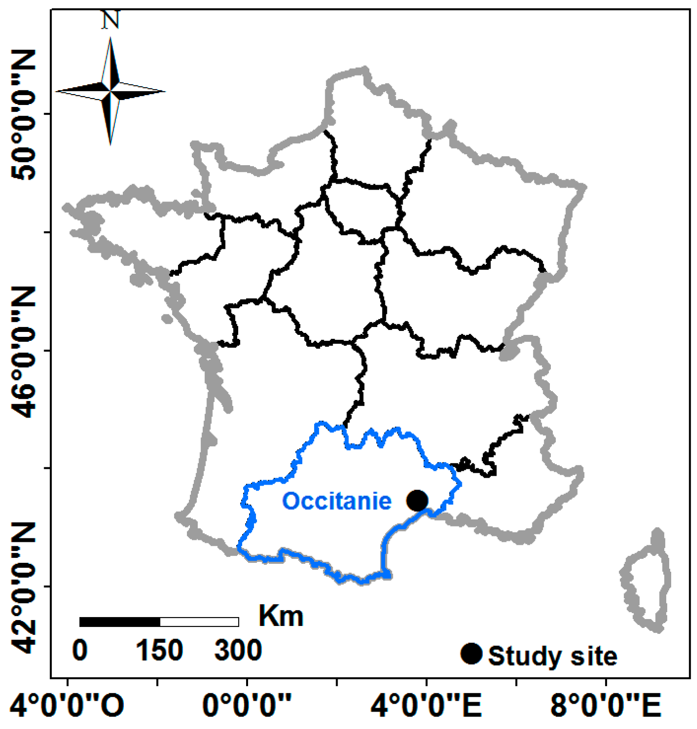
The study site is a relatively flat area located in the Occitanie region in the southwest of France (centered on 3.80° E and 43.67° N, Figure 1). The climate of the study site is Mediterranean with a rainy season between mid-October and March and an average cumulative rainfall of approximately 750 mm. The average air temperature varies between 3 °C and 29 °C. The study site is composed mainly of forest, vineyard, grassland, maize, and wheat. In total, 30 reference plots (11 grassland, 14 wheat, and 5 maize plots) between 0.6 and 9 ha in area were selected to perform our study. The topsoil texture of the reference plots is sandy loam [33] (https://www.gissol.fr/donnees/cartes/la-texture-des-horizons-superieurs-du-sol-en-france-metropolitaine-1883). A total of 12 ALOS-2/PALSAR-2, 49 Sentinel-1 (S1), and 24 Sentinel-2 (S2) images acquired between January 2017 and August 2018 were used in this study. In addition, in situ campaigns were conducted simultaneously with SAR acquisitions to collect in situ measurements of SSM in the reference plots.
2.2. Dataset Description
2.2.1. SAR Data
A total of 49 SAR images obtained from the Sentinel-1 (S1) constellation operating in the C-band (wavelength ~6 cm) were used. S1 images were downloaded from the Copernicus web site (https://scihub.copernicus.eu/dhus/#/home) for the period between January 2017 and May 2017. The S1 images were in the Interferometric Wide (IW) swath mode (primary conflict-free mode for land) with VV and VH polarizations, and they were generated from the high-resolution Level-1 Ground Range Detected product with a spatial resolution of 10 m × 10 m. For all S1 images, the study site was imaged with an incidence angle (θ) of approximately 39°.
Moreover, 12 SAR images in the L-band (wavelength ~24 cm) acquired by the Phased Array Synthetic Aperture Radar (PALSAR-2) onboard the Advanced Land Observing Satellite (ALOS-2) were used. The ALOS-2 SAR images are in mono-, dual-, and quad-polarization (Table 1). ALOS-2 data in mono- and quad-polarization have pixel sizes of 3 m × 3 m, whereas ALOS-2 data in dual-polarization have a spatial resolution of 6 m × 6 m. In this study, the L-band in VV polarization was not used because only two images contained the VV polarization.
S1 and ALOS-2 images were calibrated using the Sentinel-1 Toolbox (S1TBX) developed by the European Spatial Agency. The calibration aims to convert digital number values of ALOS-2 and S1 images into backscattering coefficients in linear units. For each reference plot, the mean backscattering coefficient in linear scale was calculated from each calibrated SAR image by averaging the σ° values of all pixels within that reference plot.
The mean of L-band backscattering coefficients acquired at various incidence angles (θ between 27.4° and 40.5°) were normalized at a given reference incidence angle (). The normalization was done using the following equation [34,35]:
where is the backscattering coefficient at the incidence angle, and is the backscattering coefficient at the incidence angle. The power index n, which depends on the nature of the target imaged and polarization (for a given radar wavelength), is defined as the slope of a linear fit between in dB and the [34,36,37,38]. In this study, was considered equal to 37°. The normalization of the backscattering coefficient was performed using Equation (1) with n-values of 3.1 for HH and 2.0 for HV. To determine these n-values, first the slope of the linear fit between in dB and was computed for each target condition (elements of our dataset with close values of SSM, root mean square surface height (Hrms), and NDVI) and each polarization. Then, for each polarization, all slope values calculated for different target conditions were averaged to determine the n-value for that polarization [34,36,37,38]. Using SAR data in the C-band, Baghdadi et al. [34] showed from a study in a wetland that the power n has higher values for HH-polarization (n ~ 2.5) compared to HV-polarization (n ~ 1.7). For the L-band in HH-polarization, Ardila et al. [38] found that the n-value varied between 0.2 and 3.4 depending on vegetation type and season with the highest occurring in savanna areas.
2.2.2. Sentinel-2 Images
A total of 24 free optical images were obtained from the S2 constellation between 01/01/2017 and 31/08/2018. The S2 images were downloaded from the Theia website at the French Land Data Center (https://www.theia-land.fr/). The Theia website provides S2 images corrected for atmospheric effects and ortho-rectified [39,40]. The NDVI maps were computed using the Near-infrared (NIR) and Red (R) bands of the S2 images (Equation (2)). From each S2 image, the NDVI pixel values within each reference plot were averaged to characterize the vegetation condition of that plot. Finally, for each reference plot, to derive NDVI values at the SAR acquisition date, a linear interpolation was performed using the NDVI values corresponding to the S2 images acquired before and after the SAR acquisition date. For the reference plots, the NDVI values ranged between 0.10 (almost bare soil) and 0.92 (vegetation height ~85 cm).
2.2.3. In Situ Measurements
In situ measurements of SSM were performed only in wheat and grassland reference plots. For maize reference plots, only the irrigation practices were recorded. For grassland and wheat plots, the SSM was measured in the top 5 cm of soil by means of a TDR (Time Domain Reflectometry) probe well calibrated using gravimetric SSM measurements. For each reference plot, twenty-five to thirty measurements of volumetric SSM well distributed in the plot, were performed within a 2-hour window of the ALOS-2 and S1 acquisition time. All SSM measurements within each plot were averaged to provide a mean value for that plot. The range of SSM values was 7.0 to 36.3 vol.%.
The soil roughness parameter defined by the root mean square surface height (Hrms) was not directly measured. However, a qualitative observation on roughness was made for each plot at each field campaign performed the same day of SAR acquisition. Roughness qualitative observations were sorted into three classes: smooth areas (sowing) with Hrms less than 1 cm, medium roughness areas (slightly plowed soil) with Hrms between 1 cm and 2 cm, and rough areas (well plowed soil) with Hrms higher than 2 cm. The roughness value attributed for each reference plot at each field campaign is certainly approximate, but our experience in collecting roughness measurements over the past 20 years let’s assume that this attributed value is fairly reliable.
For grasslands and wheat plots, two datasets were built: one for the L-band and one for the C-band (177 elements in the L-band and 335 elements in the C-band). In both datasets, each element represents a reference plot at a given SAR acquisition date with the associated mean SSM value, SAR information (mean of incidence angle and mean of backscattering coefficients), and mean NDVI-value. The majority of elements have roughness values between 1 and 2 cm. For data in L-band, 12 elements of the dataset have roughness values lower than 1 cm, 156 elements have roughness values between 1 and 2 cm, and 9 elements have roughness values higher than 2 cm. For data in the C-band, 16 elements of the dataset have roughness less than 1 cm, 268 elements have roughness between 1 and 2 cm, and 51 elements have roughness higher than 2 cm. For maize plots, the dataset contains only rainfall records and SAR data in the C-band, since the swath of SAR ALOS-2 images does not cover our maize reference plots.
3. Data Analysis
In this section, the potential of SAR signals in the C and L bands to penetrate the canopy cover of wheat and grasslands was investigated. For this investigation, the sensitivity of SAR data (C and L bands) to SSM was studied according to three classes of NDVI (NDVI < 0.4, 0.4 < NDVI < 0.7, and NDVI > 0.7), and the temporal evolution of SAR data according to SSM and NDVI variations was analyzed. Furthermore, the potential of SAR data in the C-band to penetrate the maize canopy was assessed by analyzing the temporal evolution of the C-band according to SSM and NDVI variations.
3.1. Sensitivity of L-Band to SSM for Wheat and Grasslands
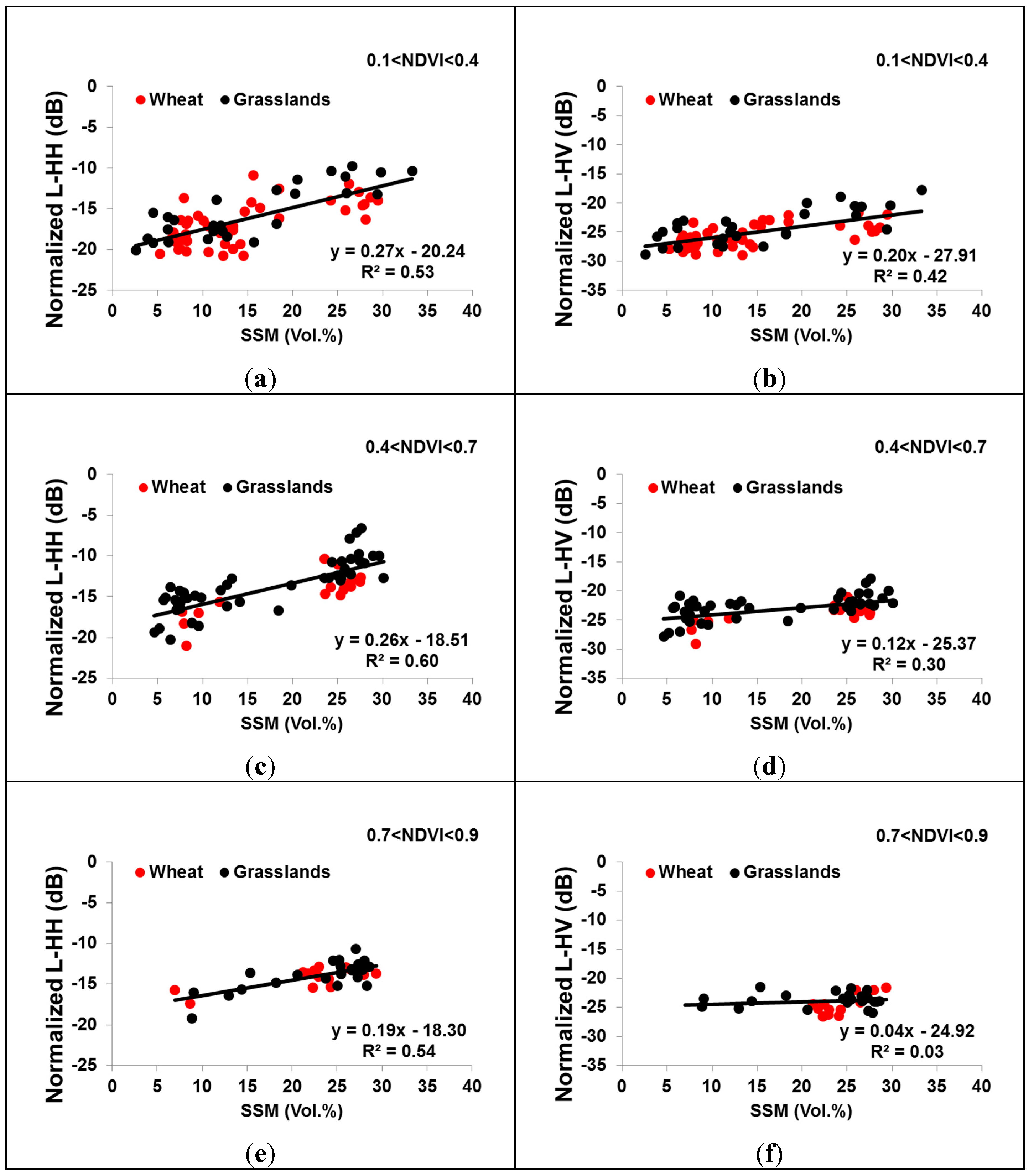
Figure 2 shows the sensitivity of the normalized SAR signal in the L-band as a function of SSM for three ranges of NDVI for wheat and grasslands plots. For NDVI between 0.1 and 0.7 (well-developed canopy cover), the sensitivity of the L-band in HH polarization (L-HH) to SSM remains unchanged (Figure 2a,c), whereas as the sensitivity of the L-band in HV polarization (L-HV) to SSM decreases with vegetation growth (Figure 2b,d). The decrease in the sensitivity of the L-HV with vegetation growth (increase in the NDVI) is related to the attenuation of the soil scattering by the vegetation volume, which is more important in HV than in HH [41,42,43,44]. Moreover, the results showed that in contrast to the L-HV, the L-HH signal is still sensitive to SSM even in the case of well-developed canopy cover (NDVI > 0.7) (Figure 2e,f). The sensitivity of the L-HH to SSM is approximately 0.27 dB/vol.% for an NDVI between 0.1 and 0.7 and decreases slightly to 0.19 dB/vol.% for an NDVI higher than 0.7 (Figure 2a,c,e). The L-HV is sensitive to SSM only in the case of NDVI values less than 0.7. The sensitivity of the L-HV is 0.20 dB/vol.% for an NDVI between 0.1 and 0.4 and 0.15 dB/vol.% for an NDVI between 0.4 and 0.7. For an NDVI above 0.7, the L-HV becomes insensitive to SSM (sensitivity = 0.04 dB/vol.%, Figure 2f). As a result, the use of the L-HH instead of the L-HV would allow better SSM estimates in the presence of vegetation cover.
3.2. Sensitivity of the C-Band to SSM for Wheat and Grassland
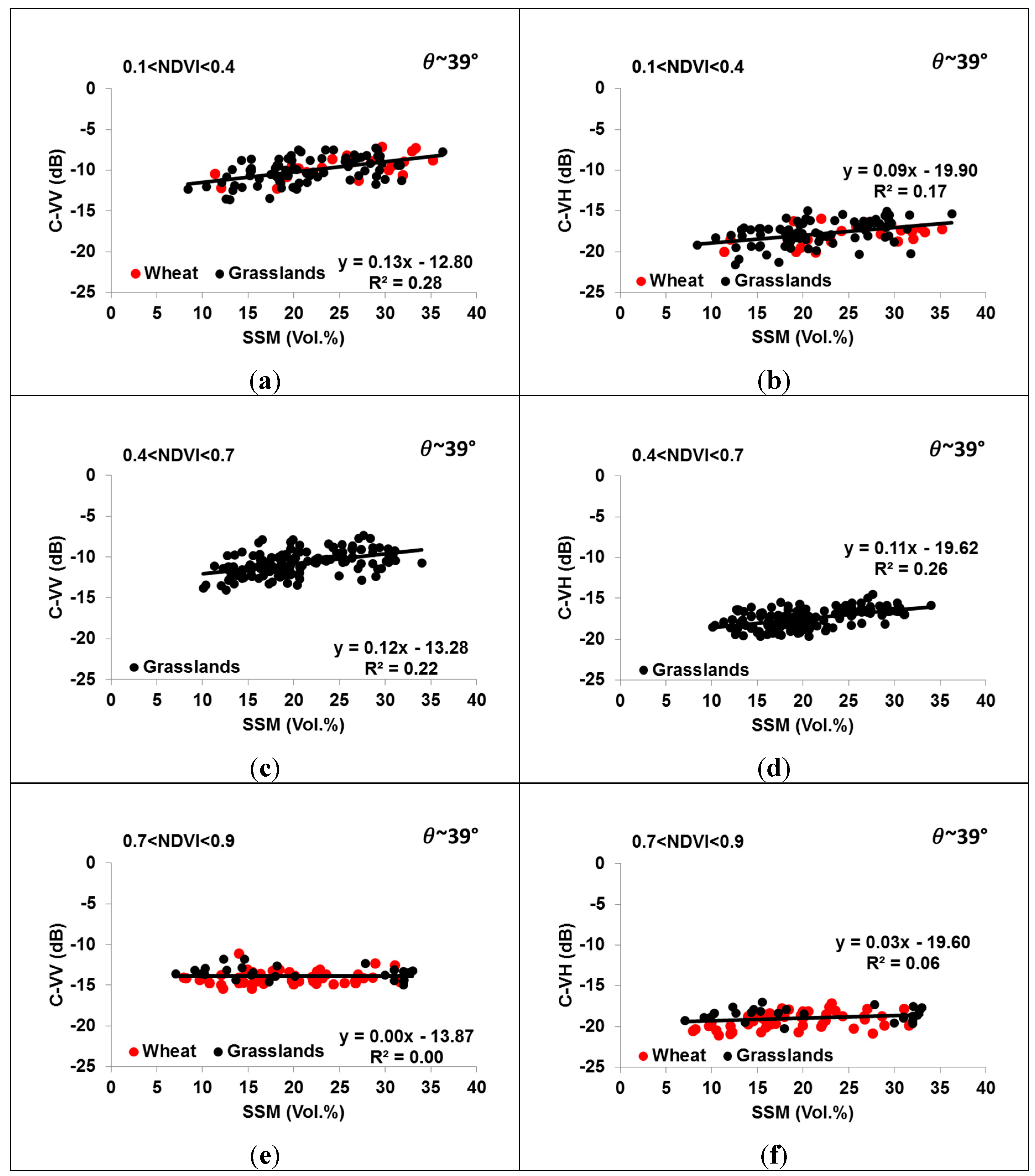
Figure 3 shows the sensitivity of the C-band in VV (C-VV) and VH (C-VH) polarizations to SSM for different NDVI ranges. For an NDVI between 0.1 and 0.7, the sensitivity of the C-VV and C-VH (incidence angle approximately 39°) to SSM is approximately 0.13 dB/vol.% and 0.10 dB/vol.%, respectively (Figure 3a–d). Moreover, Figure 3 shows that crop growth until an NDVI of 0.7 (vegetation height of 70 cm and LAI of approximately 1.5 m2/m2) does not attenuate the C-band SAR signal since the sensitivity of C-band to SSM is the same for an NDVI between 0 and 0.4 and for an NDVI between 0.4 and 0.7 (Figure 3a–d). For NDVI values higher than 0.7, the C-VV and C-VH become insensitive to SSM for SSM between 5 and 36 vol.% (Figure 3e,f). This is due to the high attenuation of C-band SAR signal by the well-developed vegetation cover. The insensitivity of C-band SAR to SSM in case of well-developed vegetation was reported in the study of Baghdadi et al. [19]. In Baghdadi et al. [19], the sensitivity of the radar signal in the C-band (VV polarization and 38°–47° incidence angles) was of 0.11 dB/vol.% and 0.05 dB/vol.% for grassland biomasses less than and greater than 1 kg/m2 (NDVI ~0.7), respectively.
3.3. Temporal Behavior of the L- and C-Bands According to the SSM and NDVI for Wheat and Grasslands
In this section, the temporal evolution of SAR backscattering in the L and C bands according to soil moisture and NDVI variations is analyzed first. Next, the behavior of the C-band backscattering during one complete growth cycle of wheat and grassland is discussed. Unfortunately, studying the behavior of the L-band backscattering during one complete growth cycle was not possible because the number of images was limited.
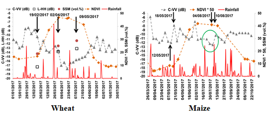
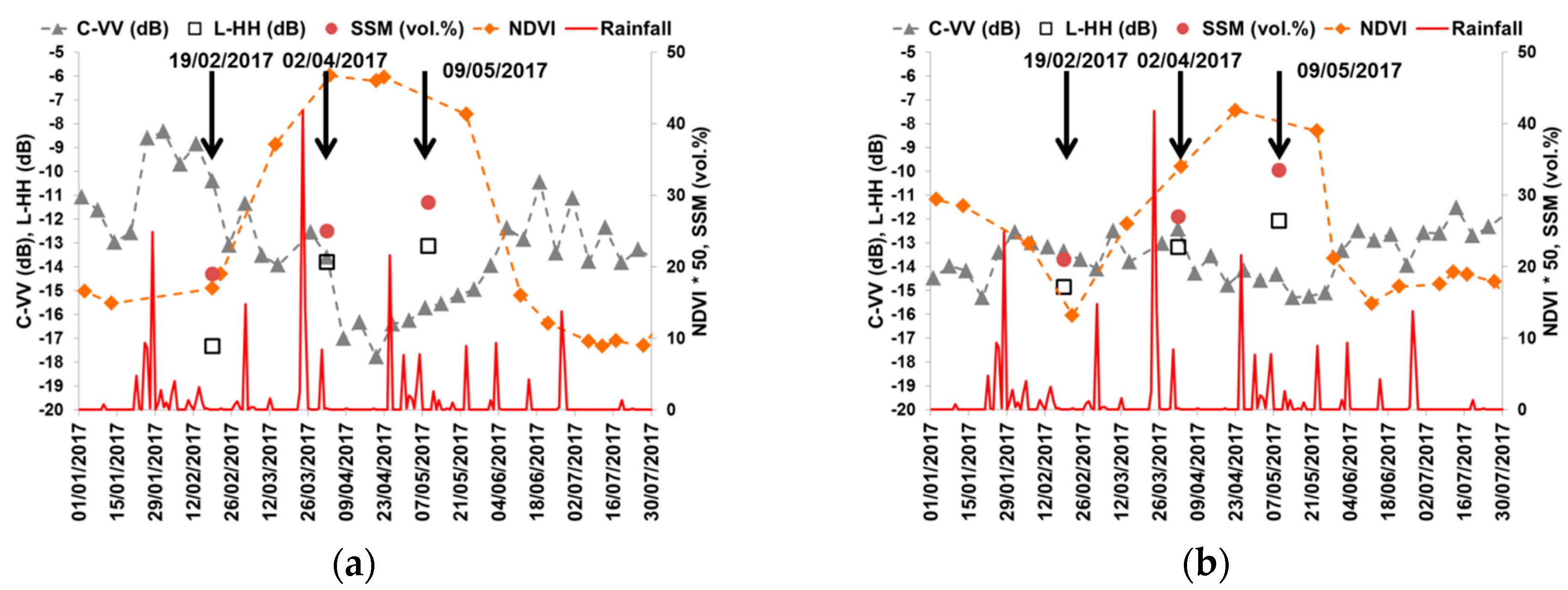
Figure 4 shows the temporal variation of radar signals in the C and L bands according to the SSM and NDVI for one wheat reference plot (Figure 4a) and one grassland reference plot (Figure 4b). For the wheat plot, Figure 4a shows that between 19/02/2017 and 02/04/2017, the SSM increases by 6.0 vol.%, the NDVI increases from 0.34 to 0.93, the C-VV decreases by 3.2 dB, and the L-HH increases by 3.5 dB. Later, between 02/04/2017 and 09/05/2017 with an NDVI approximately 0.9, the SSM increases by 4 vol.%, the C-VV decreases by 2.1 dB, and the L-HH increases by 0.7 dB. For well-developed vegetation cover (NDVI > 0.7), the decrease in the C-VV as the SSM increases indicates that attenuation caused by the canopy dominates the soil contribution. In the other hand, the increase in the L-HH with the increase in the SSM was expected since the L-HH, as shown in Figure 2, is still sensitive to soil moisture even when the canopy is well-developed (NDVI > 0.7). Therefore, in contrast to the C-VV, the L-HH incident wave penetrates the canopy layer and the L-HH backscattered wave is sensitive to SSM under the well-developed vegetation layer (NDVI > 0.7). Similar results were observed for the grassland plot (Figure 4b). For instance, between 02/04/2017 and 09/05/2017, when the NDVI is higher than 0.7, the SSM increases by 6.5 vol.%, the C-VV decreases by 1.9 dB, and the L-HH increases by 1.1 dB (Figure 4b).
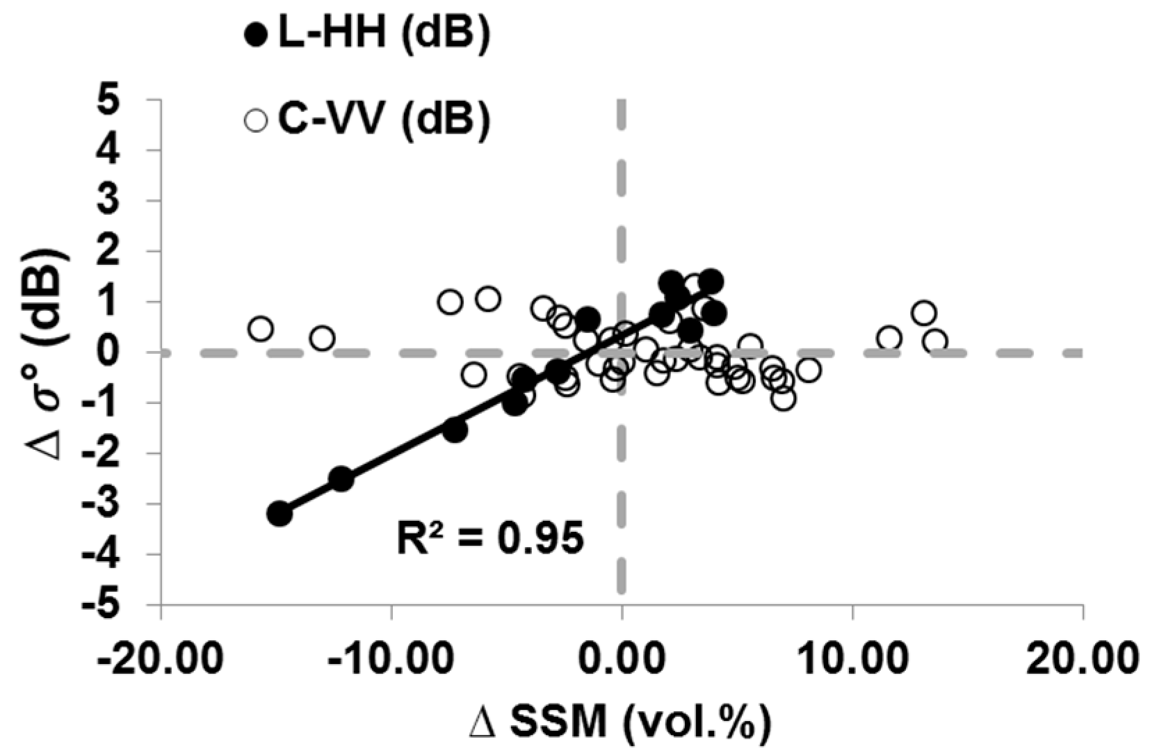
The potential of the L-HH and the inability of the C-VV to penetrate the canopy for an NDVI > 0.7 were also demonstrated for all wheat and grassland reference plots. For each reference plot with an NDVI higher than 0.7, the difference in backscattering between two successive dates (∆) was computed (the backscattering coefficient of the previous date t-1 was subtracted from that of the later date t). Then, ∆ was plotted against of the difference of the SSM (∆SSM) (Figure 5). For the L-HH, Figure 5 shows that ∆ and ∆SSM are well correlated (R2 = 0.95). This high correlation indicates that for all reference wheat and grassland plots, the L-HH is sensitive to SSM for well-developed vegetation cover (NDVI > 0.7), and the sensitivity of L-HH to SSM is almost the same for all reference plots. This demonstrates the penetration ability of the L-band into vegetation cover for an NDVI > 0.7. For the C-band and an NDVI higher than 0.7, a ∆ close to 0 is obtained for all ∆SSM between −15 vol.% and 15 vol.% (positive ∆SSM-values correspond to an increase of SSM and negative ∆SSM correspond to a decrease of SSM between two successive dates). Thus, for all reference plots, the incident C-band wave does not penetrate the vegetation layer for well-developed vegetation cover, or the C-band backscattered wave received by the SAR contains a negligible SSM contribution (impossible to detect an increase or decrease in soil moisture).
Figure 4a,b show very clearly that in the early season, approximately until the end of February (NDVI< 0.7), the radar backscattering coefficient for wheat and grassland is dominated by direct scattering from the soil. The C-VV variation is due to the SSM variation: increases following rainfall (i.e., increase in soil moisture) and decreases during a time span without rainfall due to soil evaporation (i.e., decrease in soil moisture). Between the end of February and the end of April (NDVI > 0.7), the backscattering decreases with stem elongation due to the attenuation of the direct ground scattering. This decrease is due to vertical stems and leaves that produce high absorption of the incident SAR wave associated with weak direct scattering [43,45]. The SAR signal reaches a minimum value (−17.8 dB) on 20/04/2017 (NDVI ~0.9) due to the strong attenuation produced by the longer stems. As a result, for the period extending from the end of February and the end of April, the ground backscatter attenuated by the canopy is the dominant mechanism [41,42]. At the beginning of the heading phase and during grain filling (between beginning of May and the end of June), the backscattering values start increasing due to the increase in direct scattering from ears and later from grain [42,43]. Therefore, for this period, the scattering from the upper canopy elements is the dominant mechanism [41]. From the end of June (NDVI < 0.7), the backscattering becomes sensitive to SSM due to the decrease of canopy attenuation associated with an increase of direct ground scattering. This decrease of canopy attenuation is due to vegetation drying [45]. For the grassland plot, until the beginning of April (NDVI < 0.7), the behavior of the SAR signal depends on soil moisture variations: it increases when the soil moisture increases following rainfall and decreases when the soil moisture decreases during days after a rainfall event. Between the beginning of April and the beginning of June (NDVI > 0.7), the C-VV decreases with time and is insensitive to soil moisture, which indicates that the attenuation of the SAR signal by the canopy dominates the soil contribution (the soil contribution is negligible). From the beginning of June (NDVI < 0.7), the SAR signal starts increasing due to vegetation drying and becomes sensitive to soil moisture. As a result, the C-VV backscattering is dominated by ground scattering when the NDVI of wheat and grasslands is less than 0.7, which corresponds to poorly developed and dry canopy cover. Finally, for an NDVI higher than 0.7 (very well-developed wheat and grassland cover), the C-VV is dominated by the vegetation attenuation and the soil contribution is negligible, which explains the insensitivity of the C-band to SSM for an NDVI > 0.7.
3.4. Temporal Behavior of C-Band for Maize
In this section, the behavior of the C-VV over maize is investigated. As mentioned before, studying the behavior of the L-band over maize plots was not possible because the swath of ALOS-2 images does not cover the reference maize plots. The growth cycle of maize is composed into two main stages, namely, vegetative and reproductive stages. The vegetative phase comprises planting (late April early May), end of the production of leaf collars (mid-July), and tasseling (early August). The reproductive phase comprises silking (just after tasseling), milk and dough stages (early September-mid and late September), physiological maturity (starts in October), and harvesting (end of October).
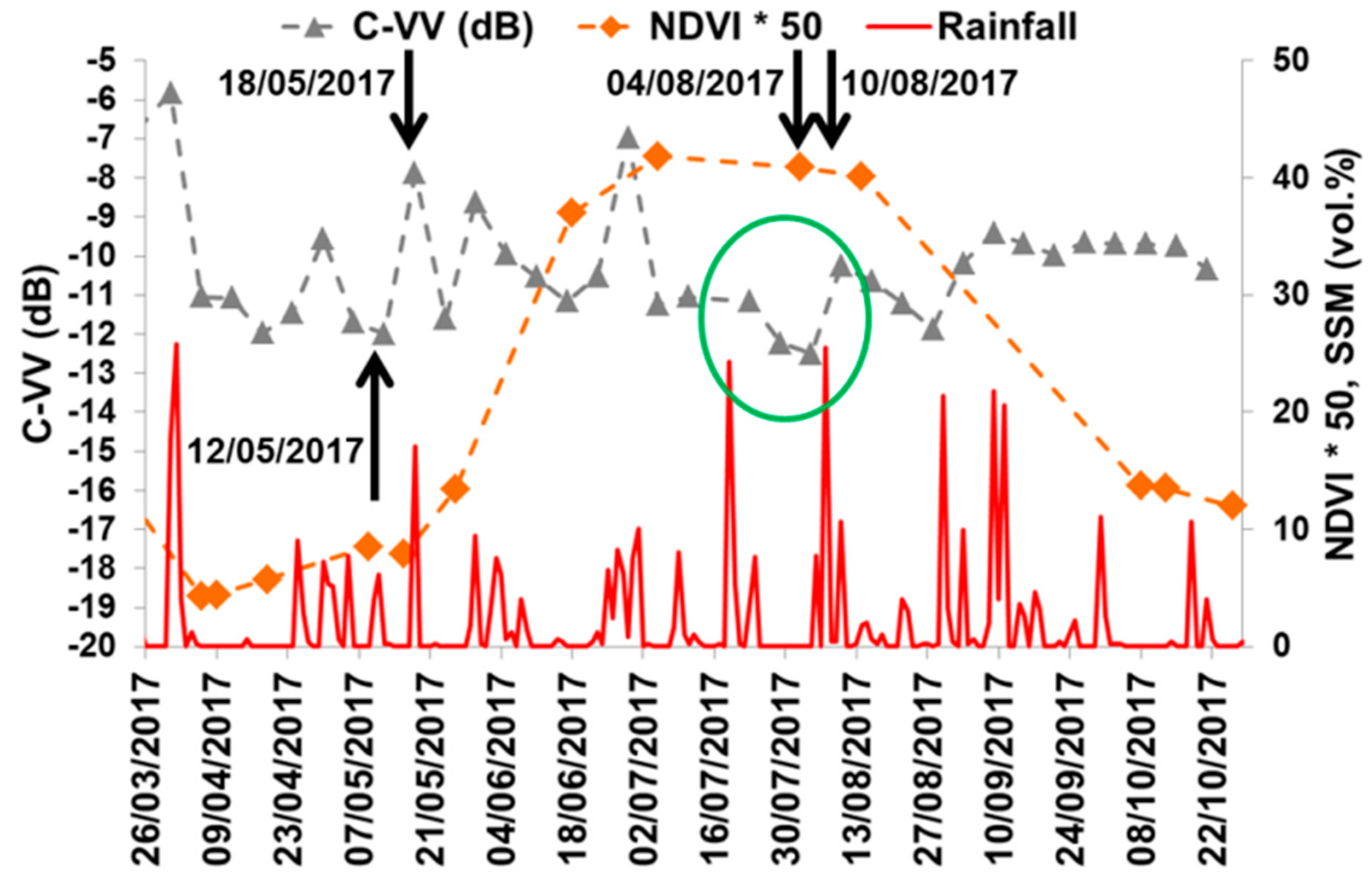
Figure 6 shows the temporal behavior of the C-VV ( of 39°) and NDVI over a maize plot. At the early stage (until the end of June), the C-VV is dominated by scattering from the ground and is sensitive to SSM variations. Indeed, the C-VV increases when the SSM increases following rainfall, then the C-VV decreases when SSM decreases during days without rainfall. For instance, the C-VV increases from −12 dB on 12/05/2018 to −7.9 dB on 18/05/2017 due to cumulative rainfall of 17.1 mm occurring in the hours before SAR acquisition on 18/05/2017. Between the end of July and the end of August the NDVI remains high (approximately 0.85) and the C-VV shows sensitivity to soil moisture. Again, the C-VV decreases with a decrease in the SSM during the time span without rainfall and increases as soil moisture increases following a rain event (green circle in Figure 6). For instance, the C-VV increases from −12.5 dB on 04/08/2017 to −10.3 dB on 10/08/2017 following two rainfall events occurring on 07/08/2017 (25.5 mm) and on 10/08/2017 (10.7 mm). The observed sensitivity of the C-VV to SSM for a well-developed maize canopy is due to the scattering along the soil-vegetation pathway that becomes significant under densely vegetated conditions [46,47]. This significant soil-vegetation pathway scattering includes a soil moisture contribution and explains the observed sensitivity of the C-VV to soil moisture [48,49]. The sensitivity of the C-VV to SSM in the presence of well-developed maize cover was reported in the study of Joseph et al. [26]. Joseph et al. [26] found that the SSM contribution to the C-band backscattering is notable even when the maize canopy is at peak biomass.
4. Conclusions
The main objective of this paper was to assess the ability of the L and C bands to penetrate the wheat, grassland, and maize canopies, which are the most frequent land covers in numerous agricultural zones in France. For wheat and grassland covers, the results showed that the L-band in HH polarization penetrates the canopy and the backscattered L-HH is sensitive to soil moisture. The sensitivity of the L-band in HH polarization is approximately 0.27 dB/vol.% and 0.19 dB/vol.% for an NDVI less than and greater than 0.7 (vegetation height of 70 cm and LAI of approximately 1.5 m2/m2), respectively. On the other hand, the C-band in both VV and HV polarization penetrates the wheat and grassland cover only when the NDVI is less than 0.7. For an NDVI less than 0.7, the C-band sensitivity to SSM is approximately 0.12 dB/vol.% for both VV and VH polarizations. At an NDVI greater than 0.7, C-band SAR is not able to penetrate the wheat and grassland covers, and thus the C-band becomes insensitive to SSM of grassland and wheat.
For maize, only the ability of the C-band to penetrate the canopy was assessed because the ALOS-2 images did not cover the maize plots. The results showed that the C-VV penetrates the maize canopy even when the maize is at peak biomass (NDVI > 0.7) and the backscattered C-VV is always sensitive to soil moisture. This is due to the significant scattering along the soil-vegetation pathway that includes a soil moisture contribution. The L-band, with a wavelength much higher than the C-band, should also penetrate the maize canopy cover. Finally, for the maize crop, the sensitivity of SAR data in L and C bands to SSM was not determined because in situ SSM measurements and ALOS-2 data were not available.
Author Contributions
M.H. and N.B. conceived and designed the experiments; M.H. and N.B. performed the experiments; M.H., N.B. and M.Z. analyzed the results; M.H. wrote the article; N.B., M.Z. and H.B. revised the paper.
Funding
This research received funding from the French Space Study Center (CNES), the National Research Institute of Science and Technology for Environment and Agriculture (IRSTEA), and the European Space Agency (ESA).
Acknowledgments
The authors wish to thank the French Space Study Center (TOSCA 2018), the National Research Institute of Science and Technology for Environment and Agriculture (IRSTEA), and the European Space Agency (project: ESA-ESTEC ITT AO/1-8845/16/CT) for supporting this work.
Conflicts of Interest
The authors declare no conflict of interest.
References
- Cepuder, P.; Nolz, R. Irrigation management by means of soil moisture sensor technologies. J. Water Land Dev. 2007, 11, 79–90. [Google Scholar] [CrossRef]
- Aubert, M.; Baghdadi, N.; Zribi, M.; Douaoui, A.; Loumagne, C.; Baup, F.; El Hajj, M.; Garrigues, S. Analysis of TerraSAR-X data sensitivity to bare soil moisture, roughness, composition and soil crust. Remote Sens. Environ. 2011, 115, 1801–1810. [Google Scholar] [CrossRef] [Green Version]
- Baghdadi, N.; Gaultier, S.; King, C. Retrieving surface roughness and soil moisture from SAR data using neural networks. In Proceedings of the Retrieval of Bio-and Geo-Physical Parameters from SAR Data for Land Applications, Sheffield, UK, 11–14 September 2001; ESTEC Publishing Division: Noordwijk, The Netherlands, 2002; Volume 475, pp. 315–319. [Google Scholar]
- Srivastava, H.S.; Patel, P.; Sharma, Y.; Navalgund, R.R. Large-area soil moisture estimation using multi-incidence-angle RADARSAT-1 SAR data. IEEE Trans. Geosci. Remote Sens. 2009, 47, 2528–2535. [Google Scholar] [CrossRef]
- Baghdadi, N.; Cresson, R.; El Hajj, M.; Ludwig, R.; La Jeunesse, I. Estimation of soil parameters over bare agriculture areas from C-band polarimetric SAR data using neural networks. Hydrol. Earth Syst. Sci. 2012, 16, 1607–1621. [Google Scholar] [CrossRef] [Green Version]
- Zribi, M.; Saux-Picart, S.; André, C.; Descroix, L.; Ottle, C.; Kallel, A. Soil moisture mapping based on ASAR/ENVISAT radar data over a Sahelian region. Int. J. Remote Sens. 2007, 28, 3547–3565. [Google Scholar] [CrossRef]
- Zribi, M.; Baghdadi, N.; Holah, N.; Fafin, O. New methodology for soil surface moisture estimation and its application to ENVISAT-ASAR multi-incidence data inversion. Remote Sens. Environ. 2005, 96, 485–496. [Google Scholar] [CrossRef]
- Zribi, M.; Gorrab, A.; Baghdadi, N. A new soil roughness parameter for the modelling of radar backscattering over bare soil. Remote Sens. Environ. 2014, 152, 62–73. [Google Scholar] [CrossRef] [Green Version]
- Tomer, S.K.; Al Bitar, A.; Sekhar, M.; Zribi, M.; Bandyopadhyay, S.; Sreelash, K.; Sharma, A.K.; Corgne, S.; Kerr, Y. Retrieval and multi-scale validation of soil moisture from multi-temporal SAR data in a semi-arid tropical region. Remote Sens. 2015, 7, 8128–8153. [Google Scholar] [CrossRef]
- Zribi, M.; Dechambre, M. A new empirical model to retrieve soil moisture and roughness from C-band radar data. Remote Sens. Environ. 2002, 84, 42–52. [Google Scholar] [CrossRef]
- Aubert, M.; Baghdadi, N.N.; Zribi, M.; Ose, K.; El Hajj, M.; Vaudour, E.; Gonzalez-Sosa, E. Toward an Operational Bare Soil Moisture Mapping Using TerraSAR-X Data Acquired Over Agricultural Areas. IEEE J. Sel. Top. Appl. Earth Obs. Remote Sens. 2013, 6, 900–916. [Google Scholar] [CrossRef] [Green Version]
- Baghdadi, N.; Saba, E.; Aubert, M.; Zribi, M.; Baup, F. Evaluation of Radar Backscattering Models IEM, Oh, and Dubois for SAR Data in X-Band Over Bare Soils. IEEE Geosci. Remote Sens. Lett. 2011, 8, 1160–1164. [Google Scholar] [CrossRef]
- Baghdadi, N.; Cresson, R.; Pottier, E.; Aubert, M.; Zribi, M.; Jacome, A.; Benabdallah, S. A potential use for the C-band polarimetric SAR parameters to characterize the soil surface over bare agriculture fields. IEEE Trans. Geosci. Remote Sens. 2012, 50, 3844–3858. [Google Scholar] [CrossRef]
- Baghdadi, N.; Aubert, M.; Zribi, M. Use of TerraSAR-X data to retrieve soil moisture over bare soil agricultural fields. IEEE Geosci. Remote Sens. Lett. 2012, 9, 512–516. [Google Scholar] [CrossRef]
- Zribi, M.; André, C.; Decharme, B. A method for soil moisture estimation in Western Africa based on the ERS scatterometer. IEEE Trans. Geosci. Remote Sens. 2008, 46, 438–448. [Google Scholar] [CrossRef]
- El Hajj, M.; Baghdadi, N.; Belaud, G.; Zribi, M.; Cheviron, B.; Courault, D.; Hagolle, O.; Charron, F. Irrigated grassland monitoring using a time series of terraSAR-X and COSMO-skyMed X-Band SAR Data. Remote Sens. 2014, 6, 10002–10032. [Google Scholar] [CrossRef]
- El Hajj, M.; Baghdadi, N.; Zribi, M.; Bazzi, H. Synergic use of Sentinel-1 and Sentinel-2 images for operational soil moisture mapping at high spatial resolution over agricultural areas. Remote Sens. 2017, 9, 1292. [Google Scholar] [CrossRef]
- El Hajj, M.; Baghdadi, N.; Zribi, M.; Belaud, G.; Cheviron, B.; Courault, D.; Charron, F. Soil moisture retrieval over irrigated grassland using X-band SAR data. Remote Sens. Environ. 2016, 176, 202–218. [Google Scholar] [CrossRef] [Green Version]
- Baghdadi, N.; EL Hajj, M.; Zribi, M.; Fayad, I. Coupling SAR C-Band and Optical Data for Soil Moisture and Leaf Area Index Retrieval Over Irrigated Grasslands. IEEE J. Sel. Top. Appl. Earth Obs. Remote Sens. 2015, 9, 1229–1243. [Google Scholar] [CrossRef]
- King, C.; Lecomte, V.; Le Bissonnais, Y.; Baghdadi, N.; Souchère, V.; Cerdan, O. Remote-sensing data as an alternative input for the ‘STREAM’runoff model. Catena 2005, 62, 125–135. [Google Scholar] [CrossRef]
- Geudtner, D.; Torres, R.; Snoeij, P.; Davidson, M.; Rommen, B. Sentinel-1 System capabilities and applications. In Proceedings of the 2014 IEEE International Geoscience and Remote Sensing Symposium (IGARSS), Quebec City, QC, Canada, 13–18 July 2014; pp. 1457–1460. [Google Scholar]
- Paloscia, S.; Pettinato, S.; Santi, E.; Notarnicola, C.; Pasolli, L.; Reppucci, A. Soil moisture mapping using Sentinel-1 images: Algorithm and preliminary validation. Remote Sens. Environ. 2013, 134, 234–248. [Google Scholar] [CrossRef]
- Mattia, F.; Balenzano, A.; Satalino, G.; Lovergine, F.; Loew, A.; Peng, J.; Wegmuller, U.; Santoro, M.; Cartus, O.; Dabrowska-Zielinska, K. Sentinel-1 high resolution soil moisture. In Proceedings of the 2017 IEEE International Geoscience and Remote Sensing Symposium (IGARSS), Fort Worth, TX, USA, 23–28 July 2017; pp. 5533–5536. [Google Scholar]
- Gao, Q.; Zribi, M.; Escorihuela, M.J.; Baghdadi, N. Synergetic use of Sentinel-1 and Sentinel-2 data for soil moisture mapping at 100 m resolution. Sensors 2017, 17, 1966. [Google Scholar] [CrossRef] [PubMed]
- Baghdadi, N.; El Hajj, M.; Zribi, M.; Bousbih, S. Calibration of the Water Cloud Model at C-Band for Winter Crop Fields and Grasslands. Remote Sens. 2017, 9, 969. [Google Scholar] [CrossRef]
- Joseph, A.T.; van der Velde, R.; O’neill, P.E.; Lang, R.; Gish, T. Effects of corn on C-and L-band radar backscatter: A correction method for soil moisture retrieval. Remote Sens. Environ. 2010, 114, 2417–2430. [Google Scholar] [CrossRef]
- Ulaby, F.T.; Moore, R.K.; Fung, A.K. Microwave Remote Sensing: Active and Passive, vol. III, Volume Scattering and Emission Theory, Advanced Systems and Applications; Artech House: Dedham, MA, USA, 1986; pp. 1797–1848. [Google Scholar]
- Kerr, Y.H.; Waldteufel, P.; Wigneron, J.-P.; Delwart, S.; Cabot, F.; Boutin, J.; Escorihuela, M.-J.; Font, J.; Reul, N.; Gruhier, C. The SMOS mission: New tool for monitoring key elements ofthe global water cycle. Proc. IEEE 2010, 98, 666–687. [Google Scholar] [CrossRef]
- Entekhabi, D.; Njoku, E.G.; Neill, P.E.; Kellogg, K.H.; Crow, W.T.; Edelstein, W.N.; Entin, J.K.; Goodman, S.D.; Jackson, T.J.; Johnson, J. The soil moisture active passive (SMAP) mission. Proc. IEEE 2010, 98, 704–716. [Google Scholar] [CrossRef]
- Narvekar, P.S.; Entekhabi, D.; Kim, S.-B.; Njoku, E.G. Soil moisture retrieval using L-band radar observations. IEEE Trans. Geosci. Remote Sens. 2015, 53, 3492–3506. [Google Scholar] [CrossRef]
- Bruscantini, C.A.; Konings, A.G.; Narvekar, P.S.; McColl, K.A.; Entekhabi, D.; Grings, F.M.; Karszenbaum, H. L-band radar soil moisture retrieval without ancillary information. IEEE J. Sel. Top. Appl. Earth Obs. Remote Sens. 2015, 8, 5526–5540. [Google Scholar] [CrossRef]
- Lievens, H.; Vernieuwe, H.; Alvarez-Mozos, J.; De Baets, B.; Verhoest, N.E. Error in radar-derived soil moisture due to roughness parameterization: An analysis based on synthetical surface profiles. Sensors 2009, 9, 1067–1093. [Google Scholar] [CrossRef]
- Sol, G. L’état des sols de France. Groupement d’intérêt scientifique sur les sols. 2011, p. 188. Available online: https://www.researchgate.net/publication/281387497_L’etat_des_sols_de_France (accessed on 13 November 2018).
- Baghdadi, N.; Bernier, M.; Gauthier, R.; Neeson, I. Evaluation of C-band SAR data for wetlands mapping. Int. J. Remote Sens. 2001, 22, 71–88. [Google Scholar] [CrossRef]
- Topouzelis, K.; Singha, S.; Kitsiou, D. Incidence angle normalization of Wide Swath SAR data for oceanographic applications. Open Geosci. 2016, 8, 450–464. [Google Scholar] [CrossRef]
- Baghdadi, N.; Boyer, N.; Todoroff, P.; El Hajj, M.; Bégué, A. Potential of SAR sensors TerraSAR-X, ASAR/ENVISAT and PALSAR/ALOS for monitoring sugarcane crops on Reunion Island. Remote Sens. Environ. 2009, 113, 1724–1738. [Google Scholar] [CrossRef]
- Mladenova, I.; Lakshmi, V.; Walker, J.P.; Panciera, R.; Wagner, W.; Doubkova, M. Validation of the ASAR global monitoring mode soil moisture product using the NAFE’05 data set. IEEE Trans. Geosci. Remote Sens. 2010, 48, 2498–2508. [Google Scholar] [CrossRef]
- Ardila, J.P.; Tolpekin, V.; Bijker, W. Angular backscatter variation in L-band ALOS ScanSAR images of tropical forest areas. IEEE Geosci. Remote Sens. Lett. 2010, 7, 821–825. [Google Scholar] [CrossRef]
- Hagolle, O.; Huc, M.; Pascual, D.V.; Dedieu, G. A multi-temporal method for cloud detection, applied to FORMOSAT-2, VENµS, LANDSAT and SENTINEL-2 images. Remote Sens. Environ. 2010, 114, 1747–1755. [Google Scholar] [CrossRef] [Green Version]
- Hagolle, O.; Huc, M.; Villa Pascual, D.; Dedieu, G. A multi-temporal and multi-spectral method to estimate aerosol optical thickness over land, for the atmospheric correction of formosat-2, Landsat, venμs and Sentinel-2 images. Remote Sens. 2015, 7, 2668–2691. [Google Scholar] [CrossRef]
- Brown, S.C.; Quegan, S.; Morrison, K.; Bennett, J.C.; Cookmartin, G. High-resolution measurements of scattering in wheat canopies-Implications for crop parameter retrieval. IEEE Trans. Geosci. Remote Sens. 2003, 41, 1602–1610. [Google Scholar] [CrossRef]
- Picard, G.; Le Toan, T.; Mattia, F. Understanding C-band radar backscatter from wheat canopy using a multiple-scattering coherent model. IEEE Trans. Geosci. Remote Sens. 2003, 41, 1583–1591. [Google Scholar] [CrossRef]
- Mattia, F.; Le Toan, T.; Picard, G.; Posa, F.I.; D’Alessio, A.; Notarnicola, C.; Gatti, A.M.; Rinaldi, M.; Satalino, G.; Pasquariello, G. Multitemporal C-band radar measurements on wheat fields. IEEE Trans. Geosci. Remote Sens. 2003, 41, 1551–1560. [Google Scholar] [CrossRef]
- Cookmartin, G.; Saich, P.; Quegan, S.; Cordey, R.; Burgess-Allen, P.; Sowter, A. Modeling microwave interactions with crops and comparison with ERS-2 SAR observations. IEEE Trans. Geosci. Remote Sens. 2000, 38, 658–670. [Google Scholar] [CrossRef]
- Del Frate, F.; Ferrazzoli, P.; Guerriero, L.; Strozzi, T.; Wegmuller, U.; Cookmartin, G.; Quegan, S. Wheat cycle monitoring using radar data and a neural network trained by a model. IEEE Trans. Geosci. Remote Sens. 2004, 42, 35–44. [Google Scholar] [CrossRef]
- Macelloni, G.; Paloscia, S.; Pampaloni, P.; Marliani, F.; Gai, M. The relationship between the backscattering coefficient and the biomass of narrow and broad leaf crops. IEEE Trans. Geosci. Remote Sens. 2001, 39, 873–884. [Google Scholar] [CrossRef]
- Chauhan, N.S.; Le Vine, D.M.; Lang, R.H. Discrete scatter model for microwave radar and radiometer response to corn: Comparison of theory and data. IEEE Trans. Geosci. Remote Sens. 1994, 32, 416–426. [Google Scholar] [CrossRef]
- Chiu, T.; Sarabandi, K. Electromagnetic scattering from short branching vegetation. IEEE Trans. Geosci. Remote Sens. 2000, 38, 911–925. [Google Scholar] [CrossRef] [Green Version]
- Stiles, J.M.; Sarabandi, K. Electromagnetic scattering from grassland. I. A fully phase-coherent scattering model. IEEE Trans. Geosci. Remote Sens. 2000, 38, 339–348. [Google Scholar] [CrossRef]
Figure 1.
Location of the study site.

Figure 2.
Sensitivity of the L-band backscattering coefficient as a function of SSM for three ranges of NDVI values. (a): L-HH and 0.1 < NDVI <0.4; (b): L-HV and 0 < NDVI <0.4; (c): L-HH and 0.4 < NDVI < 0.7; (d): L-HV and 0.4 < NDVI<0.7; (e): L-HH and 0.7 < NDVI < 0.9; (f): L-HV and 0.7 < NDVI < 0.9.

Figure 3.
Sensitivity of C-band backscattering coefficient as a function of SSM for three ranges of NDVI values. (a): C-VV and 0.1 < NDVI < 0.4; (b): C-HV and 0 < NDVI < 0.4; (c): C-VV and 0.4 < NDVI < 0.7; (d): C-HV and 0.4 < NDVI < 0.7; (e): C-VV and 0.7< NDVI < 0.9; (f): C-HV and 0.7 < NDVI < 0.9.

Figure 4.
Temporal variation of the SAR signal in the L and C bands according to in situ SSM and NDVI. (a): wheat reference plot, (b): grassland reference plot. To display NDVI and SSM values on the same axis the NDVI-values were multiplied by 50 (for instance, an NDVI-value of 0.8 corresponds to a value of 40 in Figure 4a,b). The vertical lines in red represent the rainfall events.

Figure 5.
∆(difference in between two successive dates) in the L and C bands versus ∆SSM (corresponding difference of SSM) for reference plots of wheat and grassland with an NDVI greater than 0.7. Positive ∆ and ∆SSM correspond to increases between two successive dates of and SSM, respectively.
Figure 5.
∆(difference in between two successive dates) in the L and C bands versus ∆SSM (corresponding difference of SSM) for reference plots of wheat and grassland with an NDVI greater than 0.7. Positive ∆ and ∆SSM correspond to increases between two successive dates of and SSM, respectively.

Figure 6.
Temporal behavior of the radar signal in the C-band and VV polarization over a nonirrigated maize plot. The vertical lines in red represent the rainfall events. To display NDVI and SSM values on the same axis, the NDVI-values were multiplied by 50.
Figure 6.
Temporal behavior of the radar signal in the C-band and VV polarization over a nonirrigated maize plot. The vertical lines in red represent the rainfall events. To display NDVI and SSM values on the same axis, the NDVI-values were multiplied by 50.


Table 1.
Characteristics of ALOS-2 images.
| SAR Dates dd/mm/yyyy | Polarizations | Incidence Angle (°) | Pixel Size m × m |
|---|---|---|---|
| 02/10/2016 | HH+HV | ~37.5 | 6 × 6 |
| 19/02/2017 | HH+HV | ~37.3 | 6 × 6 |
| 02/04/2017 | HH+HV+VH+VV | ~37.4 | 3 × 3 |
| 09/05/2017 | HH+HV+VH+VV | ~27.4 | 3 × 3 |
| 16/07/2017 | HH | ~40.5 | 3 × 3 |
| 15/09/2017 | HH | ~31.1 | 3 × 3 |
| 01/10/2017 | HH+HV | ~37.5 | 6 × 6 |
| 27/05/2018 | HH+HV | ~37.5 | 6 × 6 |
| 22/06/2018 | HH+HV | ~30.9 | 6 × 6 |
| 01/07/2018 | HH+HV | ~40.5 | 6 × 6 |
| 15/07/2018 | HH+HV | ~40.5 | 6 × 6 |
| 26/08/2018 | HH+HV | ~40.5 | 6 × 6 |
© 2018 by the authors. Licensee MDPI, Basel, Switzerland. This article is an open access article distributed under the terms and conditions of the Creative Commons Attribution (CC BY) license (http://creativecommons.org/licenses/by/4.0/).
Share and Cite
MDPI and ACS Style
El Hajj, M.; Baghdadi, N.; Bazzi, H.; Zribi, M. Penetration Analysis of SAR Signals in the C and L Bands for Wheat, Maize, and Grasslands. Remote Sens. 2019, 11, 31. https://doi.org/10.3390/rs11010031
AMA Style
El Hajj M, Baghdadi N, Bazzi H, Zribi M. Penetration Analysis of SAR Signals in the C and L Bands for Wheat, Maize, and Grasslands. Remote Sensing. 2019; 11(1):31. https://doi.org/10.3390/rs11010031
Chicago/Turabian StyleEl Hajj, Mohammad, Nicolas Baghdadi, Hassan Bazzi, and Mehrez Zribi. 2019. "Penetration Analysis of SAR Signals in the C and L Bands for Wheat, Maize, and Grasslands" Remote Sensing 11, no. 1: 31. https://doi.org/10.3390/rs11010031
Note that from the first issue of 2016, this journal uses article numbers instead of page numbers. See further details here.