Article

Evaluation of the SPARSE Dual-Source Model for Predicting Water Stress and Evapotranspiration from Thermal Infrared Data over Multiple Crops and Climates

1
Centre d’Etudes Spatiales de la Biosphère, Université de Toulouse, CNRS, CNES, IRD, UPS, INRA, 31401 Toulouse, France
2
EMMAH, INRA, Université d’Avignon et des Pays de Vaucluse, 84914 Avignon, France
3
HSM, Univ Montpellier, CNRS, IRD, 34090 Montpellier, France
4
Univ Paris-Sud, Laboratoire Ecologie Systématique et Evolution, AgroParisTech, CNRS, UMR 8079, Orsay, F-75231 Paris, France
5
INRA, UMR 1391 ISPA, F-33140 Villenave d’Ornon, France
*
Author to whom correspondence should be addressed.
Remote Sens. 2018, 10(11), 1806; https://doi.org/10.3390/rs10111806
Submission received: 10 October 2018 / Revised: 2 November 2018 / Accepted: 13 November 2018 / Published: 15 November 2018
(This article belongs to the Special Issue Remote Sensing of Evapotranspiration (ET))

Abstract

:
Using surface temperature as a signature of the surface energy balance is a way to quantify the spatial distribution of evapotranspiration and water stress. In this work, we used the new dual-source model named Soil Plant Atmosphere and Remote Sensing Evapotranspiration (SPARSE) based on the Two Sources Energy Balance (TSEB) model rationale which solves the surface energy balance equations for the soil and the canopy. SPARSE can be used (i) to retrieve soil and vegetation stress levels from known surface temperature and (ii) to predict transpiration, soil evaporation, and surface temperature for given stress levels. The main innovative feature of SPARSE is that it allows to bound each retrieved individual flux component (evaporation and transpiration) by its corresponding potential level deduced from running the model in prescribed potential conditions, i.e., a maximum limit if the surface water availability is not limiting. The main objective of the paper is to assess the SPARSE model predictions of water stress and evapotranspiration components for its two proposed versions (the “patch” and “layer” resistances network) over 20 in situ data sets encompassing distinct vegetation and climate. Over a large range of leaf area index values and for contrasting vegetation stress levels, SPARSE showed good retrieval performances of evapotranspiration and sensible heat fluxes. For cereals, the layer version provided better latent heat flux estimates than the patch version while both models showed similar performances for sparse crops and forest ecosystems. The bounded layer version of SPARSE provided the best estimates of latent heat flux over different sites and climates. Broad tendencies of observed and retrieved stress intensities were well reproduced with a reasonable difference obtained for most of the points located within a confidence interval of 0.2. The synchronous dynamics of observed and retrieved estimates underlined that the SPARSE retrieved water stress estimates from Thermal Infra-Red data were relevant tools for stress detection.

1. Introduction

Quantifying energy and water transfers throughout the soil-vegetation-atmosphere continuum is an essential issue to understand a wide range of processes involved in hydrological modeling, weather forecasting, and climate change impact assessment (Intergovernmental Panel on Climate Change, 2014).
Remote sensing in the thermal infrared (TIR) provides information on the surface energy balance, in particular, in relation to water stress level and on the partition of the available energy at the surface between sensible and latent heat fluxes. Available energy at the land surface, defined as the difference between net radiation (Rn) and soil heat flux (G), is mostly partitioned between sensible heat (H) and latent heat (LE) fluxes. As water needs energy to evaporate, evapotranspiration (ET) which combines evaporation from the soil and transpiration from the plants is a key component of the water and energy budgets (ET = LE/L where L is the latent heat of vaporization).
Accurate estimates of soil latent heat flux (LEs) and vegetation latent heat flux (LEv) are needed for eco-agrohydrological applications such as drought monitoring and irrigation scheduling [1,2]. Since soil evaporation is considered as a water loss that does not contribute to biomass production, optimized management in agriculture consists in maximizing the crop transpiration:evaporation ratio [3]. Separate measurements of soil evaporation and vegetation transpiration are challenging. Accurate estimation of LE partitioning is also crucial to monitor and anticipate water stress which is quantified as the complementary part to unity of the ratio between actual and potential LE [4,5]. LE in potential conditions represents a theoretical value obtained if maximum LE is reached considering actual meteorological and plant development conditions.
Numerous soil-vegetation-atmosphere transfer (SVAT) modeling approaches were developed to estimate surface fluxes at leaf and canopy levels [6]. A SVAT model is based on the simultaneous solutions of water and energy budgets to compute the temporal dynamics of various prognostic variables, such as surface fluxes, temperatures, and water content profiles of the soil and the vegetation. SVAT models require many input data such as meteorological forcing, water supply chronicles (irrigation and rain) as well as information about thermal, hydraulic, optical, and biophysical surface properties. At a local-scale, when all surface properties are generally known, they are expected to perform well [7,8]. Nevertheless, SVAT models are more difficult to implement over large areas due to uncertainties in the spatial distribution of water inputs (irrigation or rain) and soil properties at a regional scale.
Estimates of ET can also be derived from the use of the remotely-sensed land surface temperature (Trad) acquired from space in the TIR spectral domain. Conversely to SVAT models, most of these methods do not require information on water supply chronicles (irrigation and rain) and soil parameters. They rely on surface temperature, which is a relevant indicator of the water status of the surface and which can be used to retrieve the actual evapotranspiration and soil moisture status over large areas and various time scales [9]. Remotely-sensed ET products have reached a fairly satisfying level of accuracy from canopy to regional scales [2,8]. Most of the TIR-based methods employ instantaneous satellite data and compute an energy budget over the short integration period of the satellite overpass. They usually derive ET as the residual component of the surface energy balance. The most complex of these methods consider the soil and the vegetation as the two main sources of heat exchange in order to account for the partitioning of total LE into LEs and LEv [10]. A new two-source model named Soil Plant Atmosphere and Remote Sensing Evapotranspiration (SPARSE) based on the Two-Source Energy Balance (TSEB [10]) model rationale is proposed in [4]. The first innovative feature of SPARSE to the existing TSEB is similar to the post-processing step in the single-source Surface Energy Balance System (SEBS) model [11] but separately for the two components: soil and vegetation. It combines “retrieval” and “prescribed” modes by bounding each retrieved individual flux component (LEs, LEv) to its corresponding potential level deduced from running the model in prescribed potential conditions. This ensures that retrieved LEs and LEv values are below potential values considered as absolute maxima. In the usual “retrieval” mode, as in TSEB, SPARSE solves the surface energy balance equations for the soil and the canopy, which means that two unknowns (LEs and LEv) can be solved simultaneously. In the “prescribed” mode, both energy balance equations are solved to compute transpiration and evaporation rates for given stress levels (for example minimal LEs and LEv in fully stressed conditions and maximal LEs and LEv in potential conditions). In the “prescribed” mode, the surface temperature is no longer an input of the model but an output. A second key feature of SPARSE is that it provides a “patch” and a “layer” approach to describe the soil–vegetation–atmosphere interactions [12], identical to TSEB. In the “layer” approach, also referred to as the series approach, the air is well mixed within the canopy, the air temperature at the aerodynamic level is homogeneous, and the vegetation layer uniformly covers the ground. Soil and vegetation heat sources are fully coupled through a resistance network organized in series. There is one aerodynamic resistance with the air above the canopy. In the “patch” approach, also referred to as the “parallel” approach, the vegetation layer is discontinuous so that the soil interacts directly with the air above the canopy, and soil and vegetation are modeled side by side. Soil and vegetation heat sources are thermally uncoupled and fluxes are computed with a parallel resistance scheme. In the “layer” or “series” approach, soil–vegetation radiative fluxes are taken into account whereas there are no such radiation exchanges between the soil and the vegetation patches in the patch approach.
The main objective of this paper is to assess the SPARSE model predictions classically for evapotranspiration components but also for water stress. It should be noted that good retrieval values for the total latent heat flux do not guarantee that total water stress is correctly simulated. As the detection of crop water stress is crucial for efficient irrigation water management, it appeared necessary to evaluate SPARSE ability to model accurately the water status of soil and plant. We addressed four major issues:
  • Patch vs. layer approach: Even though a “patch/parallel” approach was originally proposed for sparsely vegetated semi-arid regions, and the “layer/series” approach for denser vegetation [10,13,14], there is no consensus regarding which approach offers better results in semi-arid sparse vegetation. The TSEB layer version was more robust than the TSEB patch version even though layer and patch performances were close in [15,16]. This study will bring insights on the performances of the “patch” vs. the “layer” approaches to estimate evapotranspiration and its soil component over 20 irrigated and rainfed crops, including arable crops and orchards, and various climate conditions, from temperate or Mediterranean to semi-arid and tropical climates.
  • Benefit of bounding flux retrieval: The main improvement of SPARSE is the bounding of the output fluxes by their theoretical limit values. We will test whether this improves evapotranspiration retrieval performances by comparing bounded and unbounded retrieval methods.
  • Water stress retrieval: Estimates of potential surface evapotranspiration rates are fairly well constrained by soil and vegetation biophysical properties easily obtained from visible/near-infrared remote sensing data and can explain a large amount of the information contained in the actual ET. The added value of thermal infrared (TIR) data lies in the adequate amount of information introduced by the surface temperature itself. TIR data provides information on the difference between actual and potential evapotranspiration rates (i.e., water stress) and thus soil moisture-limited evaporation and transpiration rates. We assessed the capacities of the SPARSE model to monitor water stress by comparison to water stress index chronicles derived from field data.
  • Impact of the time of overpass of a TIR satellite: One of the auxiliary goals of this paper was to investigate the impact of the time of overpass of a TIR satellite on the performance of stress retrievals in order to take into account the operational constraints imposed by the existing or future satellite platforms. At present, specific studies are missing and no consensus has been reached on the best time of overpass for stress detection.
The paper is organized as follows: First, a brief description of the SPARSE model is presented, as well as the data set used to assess the performance of the model. Then, the performances themselves are described in a “result” section showing all criteria (total fluxes, water stress level, soil evaporation efficiency). The implication for future use of the model is discussed in the last section.

2. Materials and Methods

2.1. The SPARSE Model

2.1.1. Model Description

The SPARSE model ([4] see equations in Appendix A) computes the instantaneous equilibrium surface temperatures of soil (Ts) and vegetation (Tv) (for 30-min intervals in our study, corresponding to the measurement frequency of the meteorological forcing). These temperatures are used as separate signatures of the energy budget for the soil and the vegetation. SPARSE is a generalization of the TSEB model approach which consists in linearizing the full set of energy budget equations. It implements two approaches to describe the interactions between soil-vegetation-atmosphere, namely the ‘patch’ and ‘layer’ approach which correspond to fully uncoupled and fully coupled soil–vegetation–air exchanges, respectively, using a combination equation for potential fluxes (potential transpiration and potential evaporation) and expressions of the aerodynamic resistances scheme described in [17,18,19].
Five main equations are solved simultaneously, see Equation (1). The first two, express the continuity (layer version) or the summation (patch version) of the latent and the sensible heat fluxes from the soil and the canopy to the aerodynamic level and above. The third and fourth equations represent the energy budget of the soil and the vegetation. The fifth equation describes the link between the canopy radiative surface temperature Trad that can be related to remote sensing measurements and the soil and the vegetation longwave radiative fluxes, which are related to the soil and the vegetation temperatures.
{ H = H s + H v L E = L E s + L E v R n s = G + H s + L E s R n v = H v + L E v σ T r a d 4 = R a t m R a s R a v
Ratm is the atmospheric radiation (W m−2), Ra is the net component longwave radiation (W m−2), Trad is the radiative surface temperature (°K) as observed by the satellite (which is necessary to account for the measurement waveband and the directionality of the measurements), and σ is the Stefan–Boltzmann constant. LE is the latent heat flux, H is the soil sensible heat flux, Rn is the net radiation, and G is the heat flux in the soil; indexes “s” and “v” designate the soil and the vegetation, respectively.
For LEs and LEv retrieval, Trad is known and derived from in situ thermal infrared observations. In order to compute the various fluxes of the energy balance, SPARSE follows the same approach employed by TSEB to estimate the soil evaporation and the plant transpiration from the knowledge of the sole surface temperature. As a first guess, the vegetation is supposed to transpire at a potential rate (i.e., unstressed conditions) and the system is solved to estimate LEs. If a negative value is obtained for LEs, the unstressed canopy assumption proves to be inconsistent. The vegetation is assumed to be affected by soil water stress. Then, LEs is set to a minimum value of 30 W m−2 to take into account the contribution of vapor transfer from the superficial soil layer [20]. The system is then solved to estimate the vegetation latent heat flux (LEv). If LEv is negative, fully stressed conditions are imposed for both the soil and the vegetation independently of Trad.
SPARSE can also be run in a forward mode from prescribed water stress conditions (from fully stressed to non-water-limited conditions). Actual conditions are expressed from potential conditions through the use of the efficiency coefficients which correspond to the ratio between actual and potential LE rates, βs and βv, and are functionally equivalent to surface resistances (“s” for soil, “v” for vegetation). They range between 0 and 1. If βv = 1, then the vegetation transpires at the potential rate. If βs = 1, the soil evaporation rate is that of a saturated surface. βv = 0 or βs = 0 correspond to a non-transpiring or non-evaporating surface, respectively. This prescribed mode is implemented as a final step in the retrieval mode to provide theoretical limits corresponding to maximum reachable levels of sensible and latent heat for both the soil and the vegetation.

2.1.2. Model Implementation

In our study, no calibration was performed and the parameters were arbitrarily set to realistic levels: The minimum stomatal resistance was set to 100 s m−1 for herbaceous vegetation and crops [21] and 200 s m−1 for orchard and forest [22]. The G:Rns ratio is set to 40% for an arid climate and to 25% for others [23]. The displacement height and the roughness length for momentum exchange depend on the vegetation height. Soil albedo is set to a constant value for each site, see Table 1, depending on the soil texture in accordance with the characteristics of each site.
The SPARSE surface energy balance equations required a broadband brightness temperature. When sites are not equipped with a device allowing a broadband brightness temperature measurement (if not, specified in the experimental description below) but equipped with sensors measuring the brightness temperature in the 8 to 14 μm spectral band (see below), the equations were adapted to constrain the surface energy balance in the 8 to 14 μm spectral band. To do so, atmospheric radiation, atmospheric emissivity, and surface temperature were calculated in the 8 to 14 μm atmospheric window according to [24].

2.2. Experimental Data Sets Description

Twenty data sets collected over eight crop and forest sites, see Table 1, were used to assess the performance of SPARSE. Half-hourly observations of air temperature and humidity, wind speed, net radiation, and atmospheric pressure were continuously acquired above the ground or the canopy from micro-meteorological stations over the different sites. Soil heat flux (G) was also measured at each site. Sensible (H) and latent (LE) heat fluxes were computed every 30 min from eddy-covariance systems. For sites with an energy balance closure of less than 80%, the closure was forced with the residual method and LE was computed as Rn-H-G. For other sites with an energy balance closure over 80%, the half-hourly closure was achieved with the conservation of the Bowen ratio H/LE [25]; thus, LE was computed as (Rn-G)/(1 + H/LE), see Table 1.

2.2.1. Auradé and Lamasquère Data Sets

The two cultivated plots Auradé and Lamasquère are located in the Occitanie region in France which exhibits a temperate climate. Data for Auradé were acquired in 2006 (wheat), 2007 (sunflower), and 2008 (wheat) while the data in Lamasquère were acquired in 2007, 2009, 2011, and 2013 (wheat). Surface radiative temperatures were measured with a precision infrared temperature sensor (IRTS-P, Campbell Scientific Inc, Logan, UT, USA) at 2.8 m above ground in the 6 to 14 μm spectral band in Auradé. Surface radiative temperatures were derived from longwave upwelling radiation measured by a 4-component net radiometer (CNR1 manufactured by Kipp and Zonen) at 3.65 m above ground in the 4.5 to 42 µm spectral band in Lamasquère. Leaf Area Index (LAI) was measured at key crop phenological stages (five to six measurements per crop cycle) using destructive methods and sampling schemes adapted to each crop. The leaf area was retrieved using a planimeter device. For a complete description of the site characteristics and more information on these data sets, see [26].

2.2.2. Avignon Arable Crop Data Sets

The “remote sensing and flux site” of INRA (National Institute of Agronomic Research) Avignon is located in South East France and characterized by a Mediterranean climate. Data were acquired in 2005 (peas), 2006 (wheat), 2007 (sorgho), 2008 (wheat), 2012 (wheat), and 2013 (sunflower). Surface radiative temperatures were derived from longwave upwelling radiation measured by a 4-component net radiometer (CNR1 manufactured by Kipp and Zonen) at 3 m above ground in the 4.5 to 42 µm spectral band. LAI was measured at key crop phenological stages (five to six measurements per crop cycle) using destructive methods and sampling schemes adapted to each crop. Leaf area was measured using a planimeter device. For a full description of the site characteristics and more information on these data sets, see [27].

2.2.3. Barbeau Forest Data Sets

Barbeau National Forest is a managed mature oak forest located 60 km southeast of Paris, France, in continental climatic conditions. Data covers the year 2015. Surface radiative temperatures were measured with an infrared temperature sensor (IR120, Campbell Scientific Inc., Logan, UT, USA) at 36 m above ground in the 8 to 14 μm spectral band. A complete description of the site characteristics is available in [28,29].

2.2.4. Tunisian Rainfed Wheat Data Set

The rainfed wheat was grown in 2012 in a semi-arid climate in central Tunisia, west of Kairouan. Surface temperature data were acquired with a nadir-looking Apogee thermoradiometer at 2.3 m above ground in the 8 to 14 μm spectral band. LAI was estimated with hemispherical photographs every 2 to 3 weeks depending on the phenological cycle. These data were evaluated using destructive measurements during key stages (growth and full cover). More information on that data set is available in [4].

2.2.5. Tunisian Olive Orchard Data Set

The olive orchard site is located in a semi-arid climate in central Tunisia, west of Kairouan. The site was equipped with infrared temperature sensors over the bare soil and the canopy (IR120, Campbell Scientific Inc, Logan, UT, USA) to measure the canopy and bare soil surface temperature at 9.8 m above ground in the 8 to 14 μm spectral band from March 2012. Data are available on the SEDOO OMP website with the assigned DOI: 10.6096/MISTRALS-SICMED.1479 [30].

2.2.6. Morocco Irrigated Wheat Data Set

Data for the irrigated wheat site were acquired during the 2004 growing season in the semi-arid Haouz plain in Morocco (B124 site, [31]). Surface temperature data were acquired with a nadir-looking Apogee thermoradiometer at 2 m above ground in the 8 to 14 μm spectral band. LAI was estimated with hemispherical photography every 2 to 3 weeks depending on the phenological cycle, validated by destructive measurements during key stages (growth and full cover). For a complete description of the site characteristics and more information on the data sets, see [31].

2.2.7. Niger Crop and Fallow Data Set

The study area is located 60 km east of Niamey in the South West of the Republic of Niger, characterized by a tropical semi-arid climate. It consists of two plots of around 15 ha each in the AMMA-CATCH observatory [32,33]. The two data sets used in this study were collected in 2009 over a millet field and a fallow field. Surface temperature data were acquired with 10° incidence KT15 Heitronics at 2.9 m above ground in the 8 to 14 μm spectral band. LAI was derived from hemispherical photographs. For a recent description of both the site and data set, see [34].

2.3. Assessment of Simulated Surface Water Stress

We evaluated the instantaneous estimation of water stress levels computed from SPARSE over identified stress periods. The water stress index was defined as the ratio of the difference between potential and actual evapotranspiration to potential evapotranspiration. It varies theoretically from 0 (unstressed surface) to 1 (fully stressed surface).
S = L E p o t L E x L E p o t
where LEx refers to (i) LEobs which is the observed instantaneous latent heat flux to compute “observed” water stress values or (ii) LESPARSE which is the simulated latent heat fluxes in actual conditions to compute “retrieved” water stress values from SPARSE. LEpot is the simulated latent heat flux in potential conditions. Potential evapotranspiration rates were generated from SPARSE in prescribed conditions using the Penman–Monteith formulation.
The number of stress periods was determined for each data set, see Table 1. A water stress period was identified on the following basis: Stress starts when a large deviation (>40%) between the potential evapotranspiration LEpot and the measured actual evapotranspiration rates is observed away from any rain event or any other income of water (i.e., irrigation) and ends with the next income of water. When this deviation is observed for more than 4 days in a row, we arbitrarily defined the period as stressed. As the ultimate goal of SPARSE is to retrieve ET from remotely-sensed TIR data, S was evaluated at the two nominal acquisition times by MODIS on board of TERRA and AQUA, 10:30 and 13:30.

2.4. Soil Evaporation Estimates

Individual estimates of soil evaporation and plant transpiration were not available in any site to evaluate the SPARSE simulations. Nevertheless, superficial soil moisture is a good proxy for soil evaporation, although topsoil moisture does not always react to small rainfall events and is also influenced by topsoil roots and capillarity rise of water from deeper layers. We evaluated the capacity of the SPARSE model to retrieve soil evaporation efficiency defined as βs−SPARSE (LEsSPARSE/LEspot, where LEsSPARSE and LEspot are the soil evaporation and the potential soil evaporation rate derived from running SPARSE in retrieval and prescribed potential conditions) by comparison to an independent estimation derived from the observed time series of superficial soil moisture θsurf (top 5 cm for Auradé, Lamasquère, Avignon, Tunisia, and Morocco; top 10 cm for Niger). We used the efficiency model proposed in [35] to derive the empirical soil evaporation efficiency (βs−e):
β s e = { 0.5 × [ 1 c o s ( π θ s u r f θ s a t ) ] } p
where θsat is the in situ water content at saturation and p is fixed according to soil texture to 0.5 for clay and 1 for loamy and sandy soils.
βs−SPARSE relates LEs to LEspot and ranges from 0 for a non-evaporative surface to 1 when the soil evaporation rate is equivalent to the flux from a saturated surface (see Appendix A).
L E s = β s S P A R S E ρ c p γ e s a t ( T s ) e 0 r a s
where ρcp is the product of air density and specific heat, γ the psychrometric constant, ras the soil to aerodynamic level, esat(Ts) is the saturated vapor pressure at temperature Ts, and e0 is the partial pressure of vapor at the aerodynamic level.

2.5. Experiment Design

Two sets of SPARSE simulations were derived for the layer and the patch versions of the model. In the first set, outputs were not limited by potential flux values (unbounded set) and in the second (bounded set), outputs were bounded by the potential (and fully stressed) flux rates LEspot and LEvpot, considered as the absolute maximum reachable values for evaporation and transpiration, respectively. Soil sensible and plant sensible heat fluxes were also bounded by the maximum rates in fully stressed conditions. For both versions and both sets, the performances were calculated over the entire data set for each site (from sowing to harvest for the crops; during a calendar year for others).
Total water stress estimates were also evaluated to assess the amount of information introduced by the surface temperature. The inverse mode of SPARSE was used to assess the information on moisture-limited evaporation and transpiration rates which was introduced by the surface temperature. Retrieved and “observed” water stress indexes were generated over the 20 identified stress periods.
We also compared the retrieved soil evaporation efficiency from the layer version of SPARSE to the independent empirical model (βs−e). As meteorological forcing can vary very quickly, LEpot and Trad can fluctuate significantly from one day to another and βs−SPARSE retrievals were highly variable. In order to smooth out the quick fluctuations of βs−e and the scale differences between the information provided by the integrated soil moisture measurement (top 5 cm for Auradé, Lamasquère, Avignon, Tunisia, and Morocco; top 10 cm for Niger) and the information provided by the surface temperature (relative only to the first mm of the soil), 5-day moving averages were compared. This is consistent with the potential data assimilation method of β or LE estimated from TIR data that could be used in a SVAT model for example: A smoother is more likely to outperform a sequential assimilation algorithm for short observation windows since the former will naturally smooth out the high-order fluctuations due to high-order fluctuations of Trad.

2.6. Performance Metrics

The simulations were quantitatively evaluated, comparing measured and simulated LE, H, Rn, and G from sowing to harvest for the seasonal crops and during the calendar year for others.
The simulation performance scores were quantified using the root mean square error (RMSE), the bias (Bias), and the Nash-Sutcliff Index (NI).

3. Results

3.1. Energy Balance Component Estimates

The global retrieval performances for the four energy balance components are reported in Table 2. For all data sets, the best LE estimates were obtained with the layer bounded version (global RMSE of 58 W m−2). The performances of H estimations were almost similar in the four experiments (similar RMSE and NI, but a smaller negative bias for the layer version).
RMSE, Bias, and Nash Index (NI) from the unbounded layer and patch versions for each site (from sowing to harvest for crops; during a calendar year for others) are compared in Figure 1. RMSE presented a large dispersion for LE from 30 W m−2 to 100 W m−2 depending on sites whatever the version used. Half of the sites showed negative bias for LE, H, and Rn whereas both versions of the model were systematically overestimating G. Moreover, NI for G were almost always negative. The layer unbounded version was not able to reproduce LE dynamics on the Barbeau forest site (cross symbol) whereas performances of the patch version were relatively good. Conversely, for the two wheat cultures of Lamasquère in 2007 and of Avignon in 2006, the layer version showed much better performances than the patch version. Apart from over these particular sites, the two versions showed very similar performances.
The bounded experiment provided slightly better LE estimates, with RMSE reduced by 6 W m−2, compared to the unbounded sets for the layer versions, as shown in Table 2. RMSE, Bias, and NI of the four energy balance components from the bounded layer and the unbounded layer versions were compared in Figure 2. LE retrievals were significantly better for seven sites with the bounded version compared to the non-bounded approach. LE dynamics of the Barbeau forest site were better reproduced with the bounded layer version (cross symbol). RMSE for Rn were often greater with the bounded version but biases were generally reduced. Actually, the bounded version constrains Rn with a prescribed value different of the observed one. Conversely, the unbounded version led to a simulated Rn very close in value to the measured one as Rn only depends on the incoming measured shortwave and longwave radiations and a linear expression of the surface temperature. Table 3 shows the performances of the bounded layer version for LE during each season. The RMSE and bias calculated over the fall and winter periods were the lowest over the year. These accurate performances of the model can somehow be explained by the low LE fluxes measured during these two seasons. Higher RMSE and bias were calculated over spring and, specifically, for the winter wheat cultures of Auradé, Lamasquère, and Avignon. For those crops, there was a strong overestimation by the model. In Table 3, NI were ranked into five classes to be interpreted as a non-parametric statistical test. Over the 60 seasons studied (whatever the site), 5 provided NI under 0 and attested for very poor retrievals, 14 reported between 0.25 and 0.5 (testifying for average performances), 20 reported between 0.5 and 0.75, and 15 reported over 0.75 (attesting for good to very good performances). NI showed that for two-thirds of the seasons studied, the model predicted fairly well the dynamic of LE.

3.2. Water Stress Index Estimation

During dry-downs, water stress was better retrieved from 13:30 fluxes estimations: at 10:30 only 5 RMSE values were lower than 0.2 while there were 12 values lower than 0.2 at 13:30; RMSE values at 13:30 were lower than those obtained at 10:30 for 12 periods within 16, see Table 4. The quality of water stress retrieval was highly dependent on the site and year. In general, water stress was fairly well retrieved for wheat crops. For the semi-arid sites (Tunisia, Niger, Morocco), water stress level retrievals showed RMSE values lower than 0.26 at 13:30. Figure 3 shows observed water stress estimates at 13:30 in grey and retrieved water stress estimates at 13:30 in black on four dry-downs, well-identified for the Avignon wheat in 2012 and for the Tunisian olive orchard in 2013. Missing points are related to missing data (observed data or/and inputs data). The overall magnitude of water stress is higher for the semi-arid Tunisian olive orchard than for Avignon. For the wheat crop, the observation indicates an abrupt change of stress between DOY 105 and 107, see Figure 3c whereas the SPARSE estimates displayed a smoother evolution. SPARSE properly captures the timing of water stress but could underestimate its magnitude compared to observations. For the Tunisian olive orchard, onsets of water stress were synchronous between observed and retrieved estimates. However, stress magnitude was lower for the simulated estimates, as shown in Figure 3d.

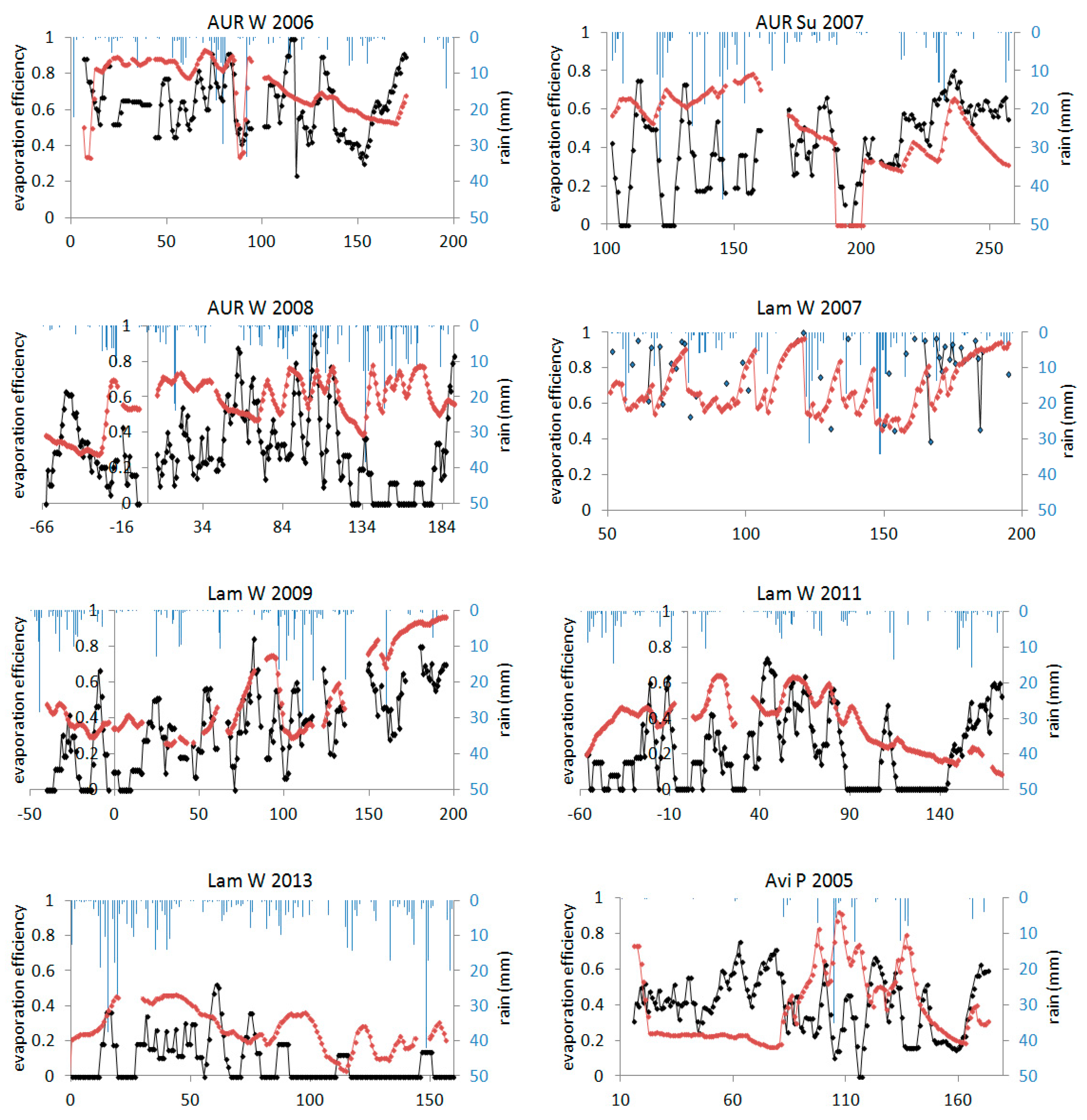
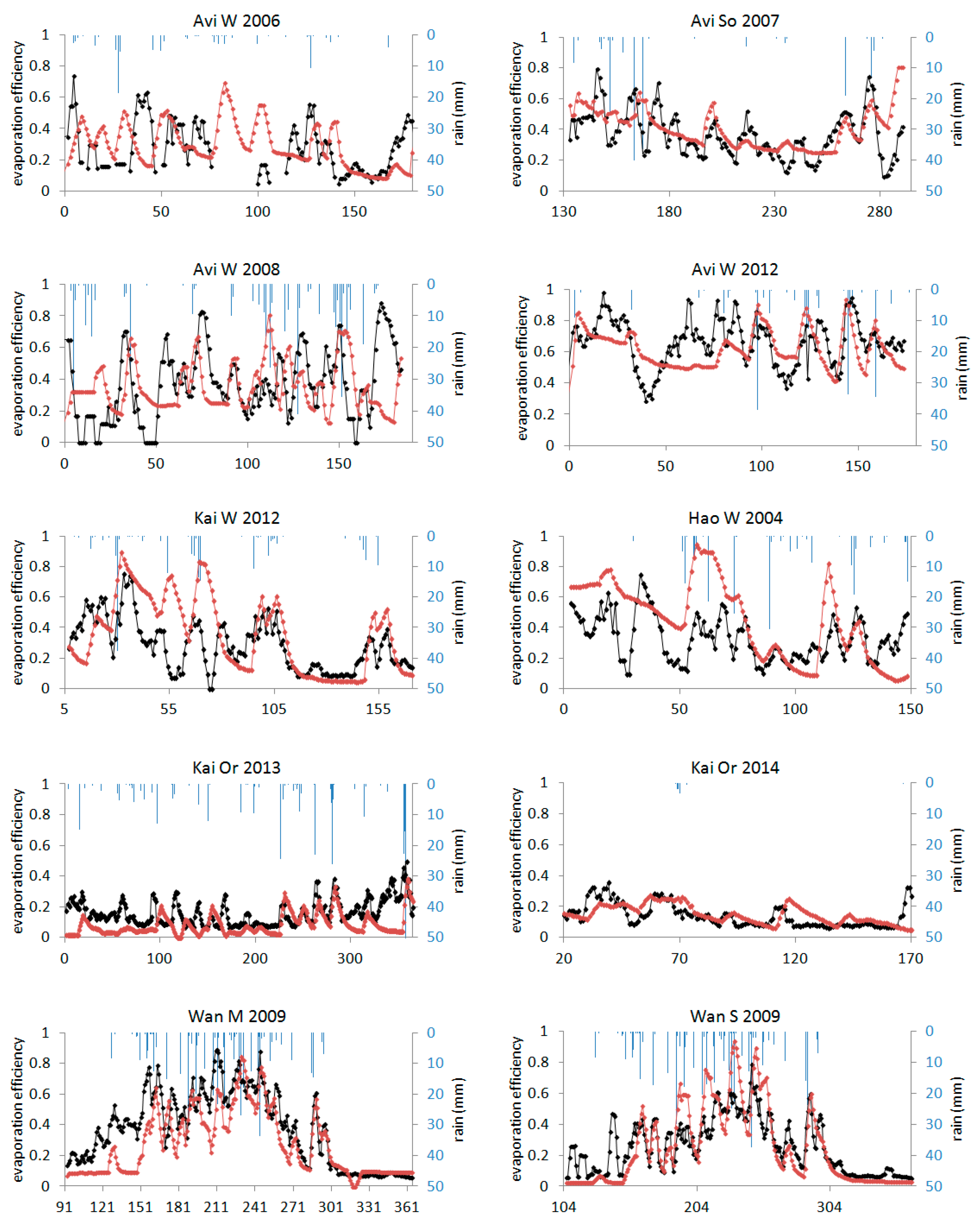
3.3. Soil Evaporation Efficiency

SPARSE showed reasonable performances for the total LE retrieval. Here, we analyze its ability to retrieve the partitioning of LE between soil and vegetation fluxes. We focused the analysis on the “layer” version which was proven to provide more accurate estimates of total LE flux. Figure 4 shows that soil evaporation efficiency amplitudes varied among crop sites (less than 0.4 for the Tunisian olive orchard and from 0.3 to 1 for the Tunisian wheat crop for example). Figure 4 also shows that SPARSE properly reproduced the seasonal magnitude, particularly the growing season dynamics (e.g., Niger site). Wetting and drying cycles are fairly retrieved. However, in several situations, there were large discrepancies in magnitude between observed and simulated efficiencies. Auradé 2008 showed significant underestimation. For Avignon in 2005, the time evolution shown by SPARSE predictions was opposite to the evolution displayed in the observations. The lower limit of SPARSE evaporation efficiency (0) resulted from a negative soil latent heat flux (LEs) (obtained because the assumption of an unstressed canopy proved to be inconsistent). In that case, the vegetation was assumed to suffer from water stress, the soil surface was assumed to have already long dried, and βs−SPARSE was zero.

4. Discussion

4.1. Overall Performance of the Dual-Source SPARSE Model

The performances of the SPARSE model for retrieving LE and its components from remotely-sensed surface temperatures were assessed over multiple crops, including orchards, and multiple climates. Over a large range of LAI values and for contrasting vegetation stress levels, the SPARSE model showed satisfactory retrieval performances of latent and sensible heat fluxes. For most of the data sets, RMSE ranged between 40 and 80 W m−2 for LE (bounded layer version) which is within the range of performances obtained by other models in the literature [15,36].

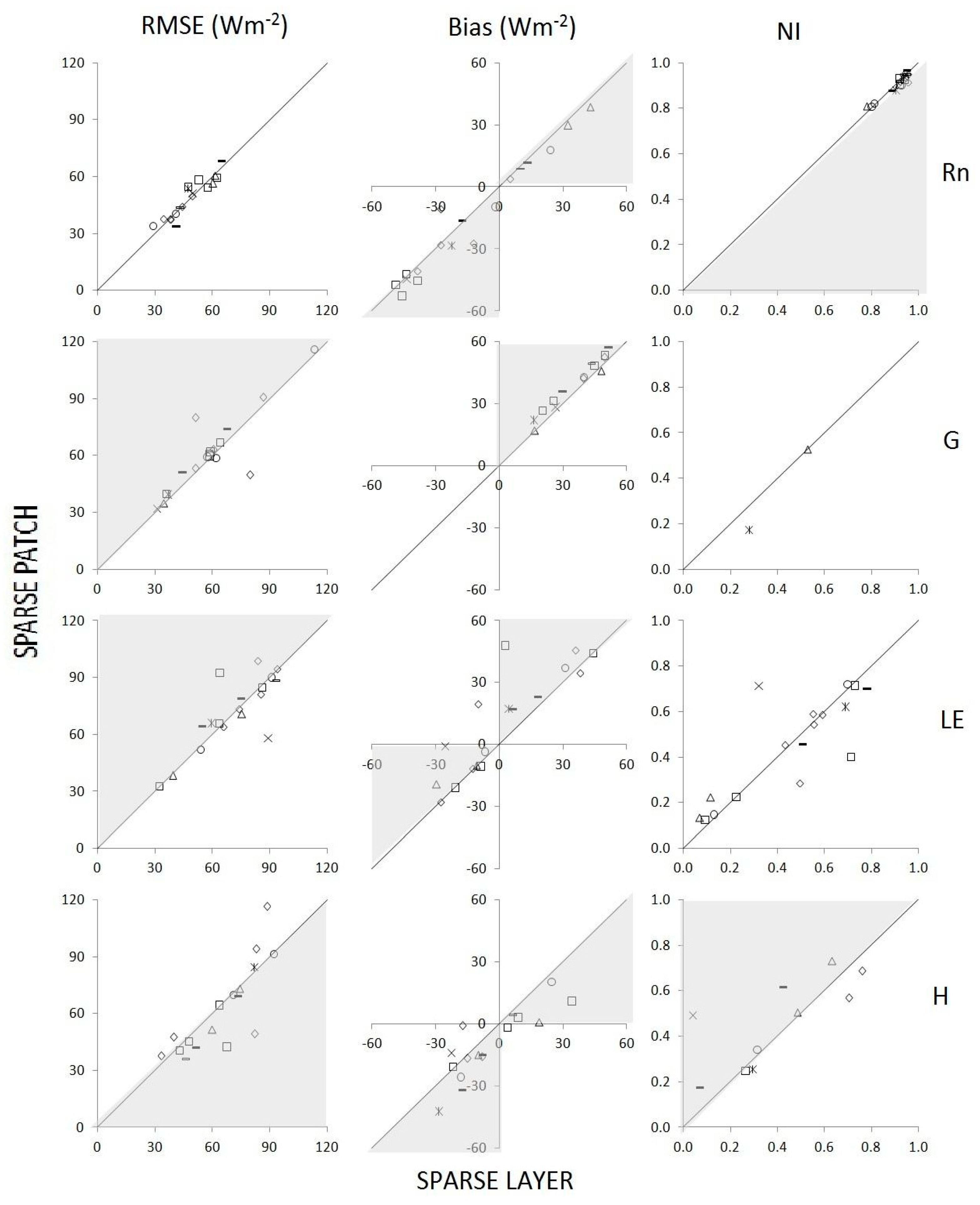
4.2. “Patch” vs. “Layer” Approach Performances

As expected for cereal covers, the layer version provided better estimates of LE than the patch version. Currently, homogeneity of cereal crops is usually well represented by such a layer approach. For sparse crops, such as orchards, or for the forest ecosystem, both patch and bounded layer schemes showed similar performances. The geometry of very sparse vegetation is better represented by the patch scheme [10] but interactions between soil and vegetation occur even for sparse vegetation [13]. A lot of usual land surface models such as CLM [37], ORCHIDEE [38], or SURFEX/MEB [39] are also based on a layer scheme. For now, using a layer or patch scheme is strongly linked to the study scale and needs to be specifically investigated to define the scale conditions corresponding to a patch approach. The patch approach could be justified at the scale where a boundary layer is fully developed over each patch and effects between patches are insignificant [40]. They also showed that the coupled model represented by the layer approach is a simplification of more complex and realistic models and that it is more widely applicable than the patch model.

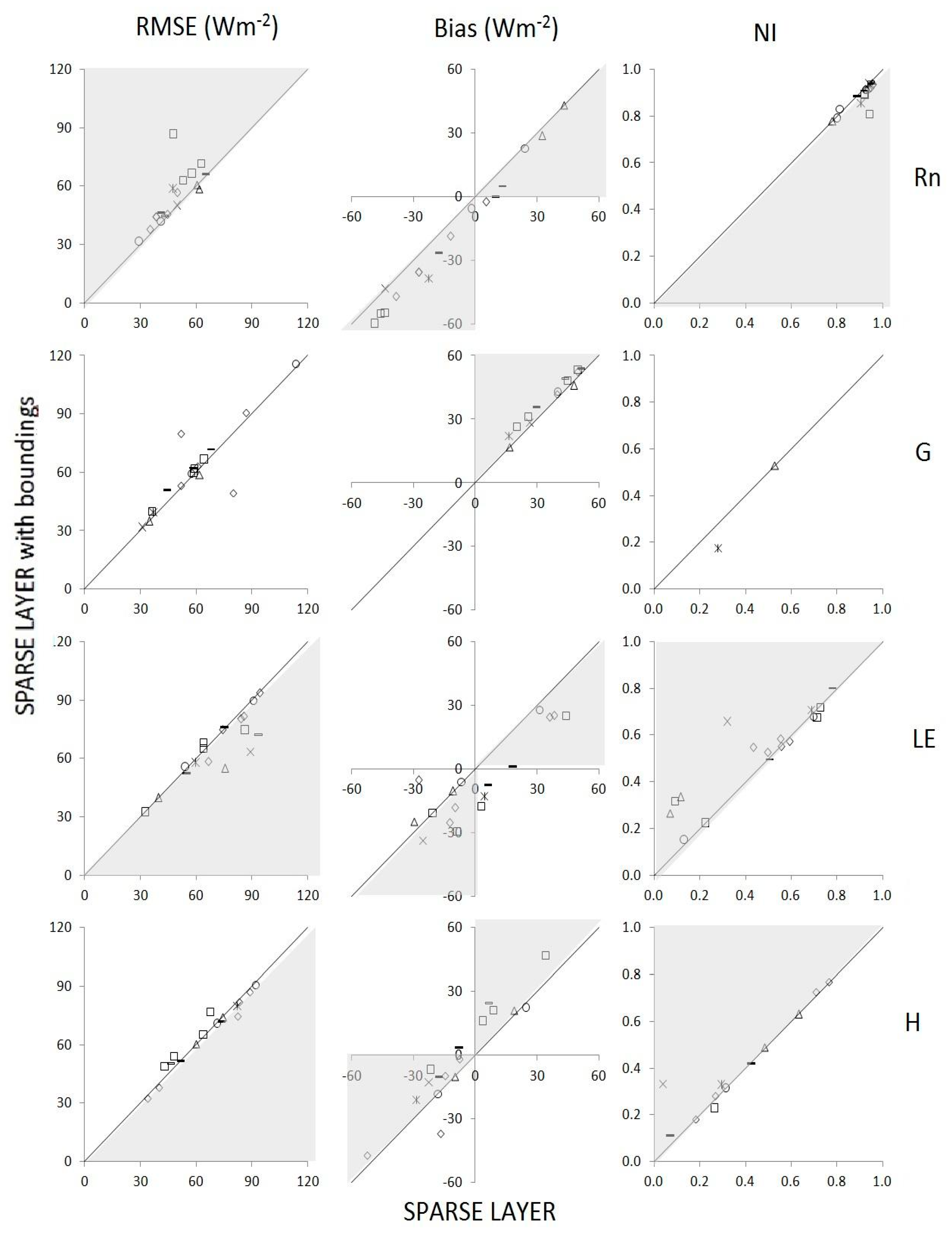
4.3. Benefit of Bounding the Flux Estimates

Bounding fluxes by realistic limiting values based on potential conditions improved latent heat flux estimates in many cases, as it allowed to correct values of evaporation and transpiration which were sometimes retrieved beyond potential levels, especially in the layer approach. These inconsistencies appeared in two types of situations: senescent vegetation and oasis effect.
  • For cereals in senescent situations at the end of the season, specific SPARSE parameter values in terms of canopy structure and stomatal conductance were not given. It is also essential to take into account the contribution of green stem and ear to the plant transpiration, especially for wheat [41,42]; this can explain the underestimation of transpiration for the Avignon and Auradé sites, see Figure 2.
  • In semi-arid areas, transpiration and particularly evaporation were retrieved beyond potential levels during periods where the soil exhibits an important dry-down (in particular the Tunisian site; Figure 2). Sensible heat transfer to the crop from drier surrounding zones led to a great overestimation of transpiration by the model because of fully coupled soil–vegetation–air exchanges in the layer version. In these situations, bounding the outputs by realistic limiting flux values ensured model robustness and reduced LE RMSE values to 30 W m−2, resulting in a reduction of global RMSE by 6 W m−2. The bounded layer version of SPARSE provided the best estimates of LE over the different sites and climates.

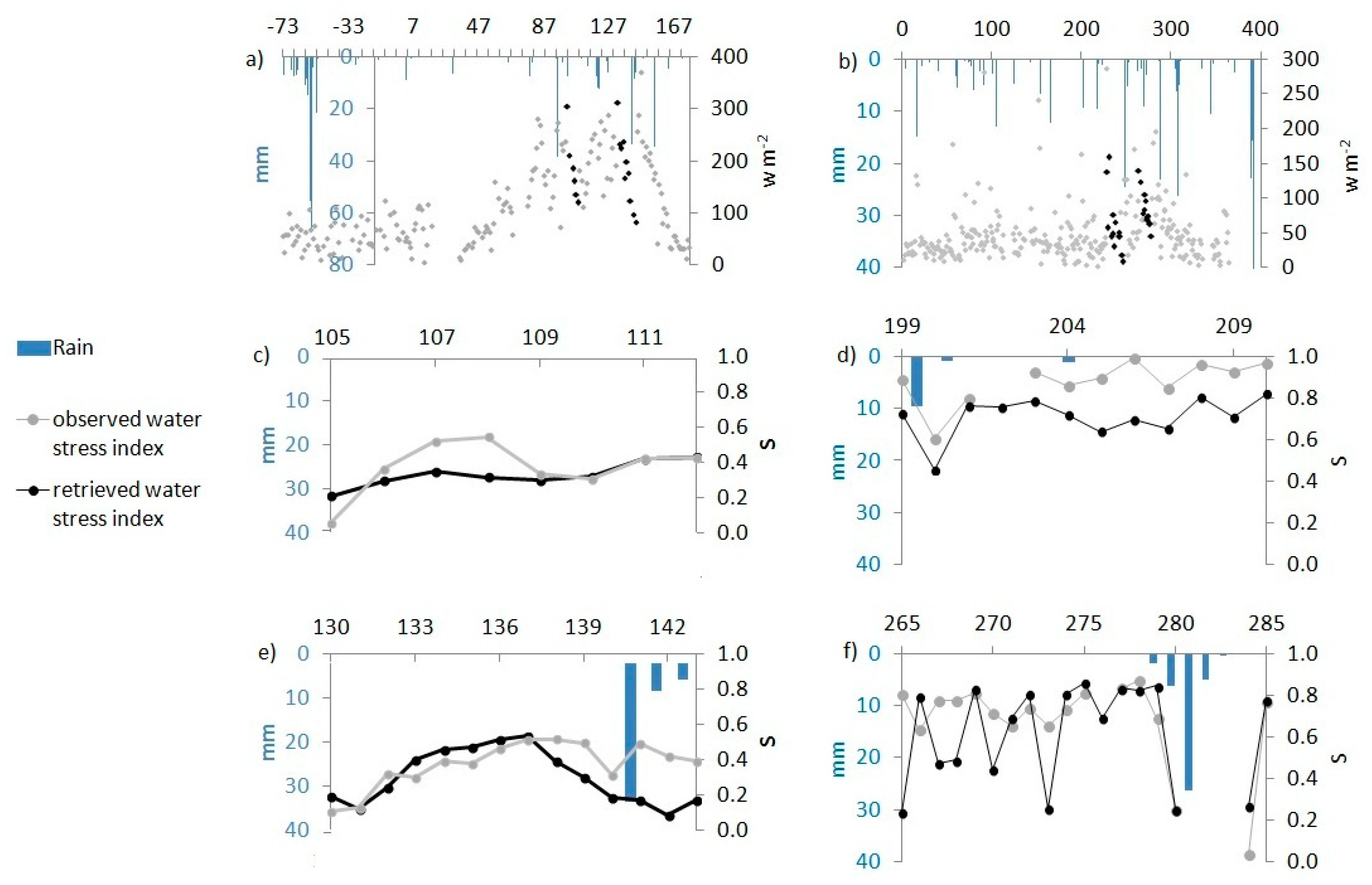
4.4. Evaluation of the Capacity of SPARSE to Monitor Water Stress

The limit of stress retrieval from noisy TIR data was pointed out by previous studies [43,44]. The differences noticed between the observed and retrieved water stress intensities remained reasonable and the dynamics were well reproduced by SPARSE, with most points located within a confidence interval of 0.2. SPARSE could then be a relevant tool for stress detection, but the hypothesis used to define water stress here did not take into account differences in the crops ability to continue to grow in water stress conditions. Further studies would consist of assimilating the water stress efficiency simulated by SPARSE in a SVAT model in order to evaluate continuous evapotranspiration rates.
Soil evaporation efficiency was evaluated amongst sites and compared to a reconstructed time series relying on observed topsoil moisture. Overall, βs−SPARSE underestimated βs−e which was a consequence of the two different approaches used to compute soil evaporation efficiencies. βs−SPARSE is not influenced by the same parameters as βs−e. Indeed, βs−e depends on the 5-cm topsoil moisture, a time-continuous variable, whose dynamics are strongly linked to large rain events while βs−SPARSE is mostly related to the porous network in direct contact with the atmosphere. Besides, βs−SPARSE and LEpot are strongly impacted by a quick change in the meteorological forcing. Trad is very sensitive to changes in atmospheric turbulence [45] whereas θ5cm, and then βs−e, are less reactive to these fluctuations. In our study, no calibration was performed and the parameters were arbitrarily set to realistic levels. This is consistent with the potential use of this model which aims at estimating LE and retrieving water stress estimations routinely from remote-sensing data with no additional calibration.
An additional issue is related to the uncertainty in the input variable, Trad. Actually, many uncertainties and errors are known to affect the remotely-sensed surface temperature, including atmospheric correction and emissivity settings [24,46] in addition to the directional dependence of Trad [47,48,49]. Particularly, angular emissivity effects can be important over heterogeneous cover where emission depends on many different individual emitters with contrasting emissivities. The TIR anisotropy comes from the heterogeneity of the observed object combined with a particular viewing angle. For sparse vegetations, directional effects can be important due to the soil contribution [48,49]. Moreover, Trad retrieval can be affected by surface layer turbulence which can generate important temporal fluctuations [45]. At the end of almost every season (except for Niger, Lamasquère 2009 and 2013 and Tunisian wheat 2012), βs−SPARSE differed greatly from the βs−e as it remained close to the potential rate. This could be related to the estimation of transpiration during the senescent period which is not properly simulated by SPARSE. Changes in soil-vegetation radiative exchanges and in canopy stomatal conductance occurring during senescence can lead to confusion over the transpiration:evaporation partition. Soil evaporation efficiencies derived from SPARSE were reasonably well retrieved for very sparse vegetation sites (Niger sites and olive orchard). In those sites, the coupling between surface temperature and evaporation reduction is properly simulated by SPARSE independent of the assumption on the water status of the vegetation.

4.5. Potential to be Driven by Earth Observation Data

One of the goals of this paper was to investigate the impact of the overpass time of a TIR satellite on the performance stress retrievals in order to take into account the operational constraints imposed by existing or future satellite platforms. The optimum time of overpass between the two tested in this work (10:30 and 13:30) was 13:30, which is in agreement with the theoretical study described in [43] based on an analytical estimation of peak latent heat flux as a response to a sinusoidal radiation forcing.

5. Conclusions

SPARSE showed satisfactory retrieval performances of latent and sensible heat fluxes, and the opportunity to bound fluxes by realistic limiting values based on potential conditions improved latent heat flux estimates in many cases, especially, in the layer approach in senescent situations at the end of the season and in semi-arid areas where transpiration and particularly evaporation were retrieved beyond potential levels.
The soil evaporation efficiencies estimated by SPARSE should be tested in order to be used to retrieve information on irrigation amount or precipitation inputs from TIR acquisitions.
Most models using information in the TIR domain like SPARSE rely on data acquired once a day within the constraints of the time of the satellite overpass, the revisit frequency, and the cloud cover. Consequently, the diurnal cycle of the energy budget is not accounted for and SPARSE will compute an instantaneous energy budget at the time of the satellite overpass and provide a single instantaneous latent heat flux. As a daily accumulation is usually required for hydrological applications for monitoring water stress, daily and seasonal LE need to be reconstructed from these retrieval instantaneous values. In order to encounter and evaluate the potential of SPARSE outputs with TIR acquisitions for the reconstruction of a continuous data set, future work will assess the impact of uncertainty on SPARSE model performances over operational methods to reconstruct ET at a daily and seasonal scale in order to fairly monitor water stress and irrigation.

Author Contributions

Data processing, data analysis, and results interpretation, E.D.; data analysis and results interpretation, G.B.; Avignon data processing, analysis, and discussions, S.G.; Auradé and Lamothe data processing and analysis, A.B. and T.T.; Barbeau data processing and analysis, K.S.; ideas and discussions, A.O., J.D. and J.-P.L.

Funding

This work was mostly supported by the French Space Agency (CNES) through TOSCA project PRECOSTRESS.

Conflicts of Interest

The authors declare no conflict of interest.

Appendix A

Basic equations of the SPARSE “layer” model
Net solar radiation on the soil is:
R g s = ( 1 α s ) ( 1 f c ) 1 f c α s α v R g
Net solar radiation on the vegetation is:
R g v = ( 1 α v ) f c [ 1 + α s ( 1 f c ) 1 f c α s α v ] R g
Net longwave radiation for the soil is:
R a s = a n s σ T s 4 + b n s σ T v 4 + c n s
Net longwave radiation for the vegetation is:
R a v = a n v σ T s 4 + b n v σ T v 4 + c n v
where:
a n s = ε s [ ( 1 f c ) + ε v f c ] 1 f c ( 1 ε s ) ( 1 ε v ) b n s = a n v = ε v ε s f c 1 f c ( 1 ε s ) ( 1 ε v ) c n s = ( 1 f c ) ε s R a t m 1 f c ( 1 ε s ) ( 1 ε v ) b n v = f c ε v [ 1 + ε s + ( 1 f c ) ( 1 ε s ) 1 f c ( 1 ε s ) ( 1 ε v ) ] c n v = f c ε v R a t m [ 1 + ( 1 f c ) ( 1 ε s ) 1 f c ( 1 ε s ) ( 1 ε v ) ]
(αs and εs are the albedo and the emissivity of the soil, αv and εv are the albedo and the emissivity of the canopy, and Rg is the global incoming radiation; the vegetation cover fraction is f c = 1 e 0.5 L A I / cos φ where φ is the view zenith angle; atmospheric radiation is R a t m = 1.24 ( e a / T a ) 1 / 7 σ T a 4 where Ta and ea are the temperature and the vapor pressure of the air, respectively).
The various fluxes of the system of Equation (1) are expressed as:
R n s = R g s + R a s ;   G = ξ   R n s ;   R n v = R g v + R a v H s = ρ c p T s T 0 r a s ,   H v = ρ c p T v T 0 r a v   e t   H = ρ c p T 0 T a r a L E s = ρ c p γ β s e s a t ( T s ) e 0 r a s ,   L E v = ρ c p γ β v e s a t ( T v ) e 0 r a v + r s t m i n   e t   L E = ρ c p γ e 0 e a r a
where ra, ras, and rav are aerodynamic resistances between the aerodynamic level and the reference level, the soil and the aerodynamic level, and the vegetation and the aerodynamic level, respectively, while rstmin is the minimum stomatal resistance; T0 and e0 are the temperature and the vapor pressure at the aerodynamic level, respectively; the two unknowns, Ts and Tv, as well as the soil evaporation efficiency βs (or the transpiration βv if the retrieved βs is lower than a minimum value corresponding to LEs = 30 W/m2), are solved simultaneously by inverting the system of Equation (1).

References

  1. Er-Raki, S.; Chehbouni, A.; Boulet, G.; Williams, D.G. Using the dual approach of FAO-56 for partitioning ET into soil and plant components for olive orchards in a semi-arid region. Agric. Water Manag. 2010, 97, 1769–1778. [Google Scholar] [CrossRef] [Green Version]
  2. Kustas, W.; Anderson, M. Advances in thermal infrared remote sensing for land surface modeling. Agric. For. Meteorol. 2009, 149, 2071–2081. [Google Scholar] [CrossRef]
  3. Evett, S.R.; Tolk, J.A. Introduction: Can Water Use Efficiency Be Modeled Well Enough to Impact Crop Management? Agron. J. 2009, 101, 423–425. [Google Scholar] [CrossRef]
  4. Boulet, G.; Mougenot, B.; Lhomme, J.-P.; Fanise, P.; Lili-Chabaane, Z.; Olioso, A.; Bahir, M.; Rivalland, V.; Jarlan, L.; Merlin, O.; et al. The SPARSE model for the prediction of water stress and evapotranspiration components from thermal infra-red data and its evaluation over irrigated and rainfed wheat. Hydrol. Earth Syst. Sci. 2015, 4653–4672. [Google Scholar] [CrossRef] [Green Version]
  5. Hain, C.R.; Mecikalski, J.R.; Anderson, M.C. Retrieval of an Available Water-Based Soil Moisture Proxy from Thermal Infrared Remote Sensing. Part I: Methodology and Validation. J. Hydrometeorol. 2009, 10, 665–683. [Google Scholar] [CrossRef]
  6. Olioso, A.; Chauki, H.; Courault, D.; Wigneron, J.-P. Estimation of Evapotranspiration and Photosynthesis by Assimilation of Remote Sensing Data into SVAT Models. Remote Sens. Environ. 1999, 68, 341–356. [Google Scholar] [CrossRef]
  7. Chirouze, J.; Boulet, G.; Jarlan, L.; Fieuzal, R.; Rodriguez, J.C.; Ezzahar, J.; Er-Raki, S.; Bigeard, G.; Merlin, O.; Garatuza-Payan, J.; et al. Intercomparison of four remote-sensing-based energy balance methods to retrieve surface evapotranspiration and water stress of irrigated fields in semi-arid climate. Hydrol. Earth Syst. Sci. 2014, 18, 1165–1188. [Google Scholar] [CrossRef] [Green Version]
  8. Olioso, A.; Inoue, Y.; Ortega-FARIAS, S.; Demarty, J.; Wigneron, J.-P.; Braud, I.; Jacob, F.; Lecharpentier, P.; OttlÉ, C.; Calvet, J.-C.; et al. Future directions for advanced evapotranspiration modeling: Assimilation of remote sensing data into crop simulation models and SVAT models. Irrig. Drain. Syst. 2005, 19, 377–412. [Google Scholar] [CrossRef]
  9. Boulet, G.; Chehbouni, A.; Gentine, P.; Duchemin, B.; Ezzahar, J.; Hadria, R. Monitoring water stress using time series of observed to unstressed surface temperature difference. Agric. For. Meteorol. 2007, 146, 159–172. [Google Scholar] [CrossRef] [Green Version]
  10. Norman, J.M.; Kustas, W.P.; Humes, K.S. Source approach for estimating soil and vegetation energy fluxes in observations of directional radiometric surface temperature. Agric. For. Meteorol. 1995, 77, 263–293. [Google Scholar] [CrossRef]
  11. Su, Z. The Surface Energy Balance System (SEBS) for estimation of turbulent heat fluxes. Hydrol. Earth Syst. Sci. 2002, 6, 85–100. [Google Scholar] [CrossRef] [Green Version]
  12. Lhomme, J.P.; Montes, C.; Jacob, F.; Prévot, L. Evaporation from Heterogeneous and Sparse Canopies: On the Formulations Related to Multi-Source Representations. Bound.-Layer Meteorol. 2012, 144, 243–262. [Google Scholar] [CrossRef]
  13. Blyth, E.M. Using a simple SVAT scheme to describe the effect of scale on aggregation. Bound.-Layer Meteorol. 1995, 72, 267–285. [Google Scholar] [CrossRef]
  14. Verhoef, A.; De Bruin, H.A.R.; Van Den Hurk, B.J.J.M. Some Practical Notes on the parameter kB-1 for Sparse Vegetation. Am. Meteorol. Soc. 1997, 36, 560–572. [Google Scholar] [CrossRef]
  15. Li, F.; Kustas, W.P.; Prueger, J.H.; Neale, C.M.U.; Jackson, T.J. Utility of Remote Sensing–Based Two-Source Energy Balance Model under Low- and High-Vegetation Cover Conditions. J. Hydrometeorol. 2005, 6, 878–891. [Google Scholar] [CrossRef]
  16. Morillas, L.; García, M.; Nieto, H.; Villagarcia, L.; Sandholt, I.; Gonzalez-Dugo, M.P.; Zarco-Tejada, P.J.; Domingo, F. Using radiometric surface temperature for surface energy flux estimation in Mediterranean drylands from a two-source perspective. Remote Sens. Environ. 2013, 136, 234–246. [Google Scholar] [CrossRef] [Green Version]
  17. Choudhury, B.J.; Monteith, J.L. A four-layer model for the heat budget of homogeneous land surfaces. Q. J. R. Meteorol. Soc. 1988, 114, 373–398. [Google Scholar] [CrossRef]
  18. Shuttleworth, W.J.; Gurney, R.J. The theoretical relationship between foliage temperature and canopy resistance in sparse crops. Q. J. R. Meteorol. Soc. 1990, 116, 497–519. [Google Scholar] [CrossRef]
  19. Shuttleworth, W.J.; Wallace, J.S. Evaporation from sparse crops-an energy combination theory. Q. J. R. Meteorol. Soc. 1985, 111, 839–855. [Google Scholar] [CrossRef]
  20. Boulet, G.; Braud, I.; Vauclin, M. Study of the mechanisms of evaporation under arid conditions using a detailed model of the soil–atmosphere continuum. Application to the EFEDA I experiment. J. Hydrol. 1997, 193, 114–141. [Google Scholar] [CrossRef]
  21. Gentine, P.; Entekhabi, D.; Chehbouni, A.; Boulet, G.; Duchemin, B. Analysis of evaporative fraction diurnal behaviour. Agric. For. Meteorol. 2007, 143, 13–29. [Google Scholar] [CrossRef] [Green Version]
  22. Masson, V.; Champeaux, J.-L.; Chauvin, F.; Meriguet, C.; Lacaze, R. A Global Database of Land Surface Parameters at 1-km Resolution in Meteorological and Climate Models. J. Clim. 2003, 16, 1261–1282. [Google Scholar] [CrossRef] [Green Version]
  23. Kustas, W.P.; Daughtry, C.S.T. Estimation of the soil heat flux/net radiation ratio from spectral data. Agric. For. Meteorol. 1990, 49, 205–223. [Google Scholar] [CrossRef]
  24. Olioso, A. Estimating the difference between brightness and surface temperatures for a vegetal canopy. Agric. For. Meteorol. 1995, 72, 237–242. [Google Scholar] [CrossRef]
  25. Twine, T.E.; Kustas, W.P.; Norman, J.M.; Cook, D.R.; Houser, P.R.; Meyers, T.P.; Prueger, J.H.; Starks, P.J.; Wesely, M.L. Correcting eddy-covariance flux underestimates over a grassland. Agric. For. Meteorol. 2000, 103, 279–300. [Google Scholar] [CrossRef] [Green Version]
  26. Béziat, P.; Ceschia, E.; Dedieu, G. Carbon balance of a three crop succession over two cropland sites in South West France. Agric. For. Meteorol. 2009, 149, 1628–1645. [Google Scholar] [CrossRef] [Green Version]
  27. Garrigues, S.; Olioso, A.; Calvet, J.C.; Martin, E.; Lafont, S.; Moulin, S.; Chanzy, A.; Marloie, O.; Buis, S.; Desfonds, V.; et al. Evaluation of land surface model simulations of evapotranspiration over a 12-year crop succession: Impact of soil hydraulic and vegetation properties. Hydrol. Earth Syst. Sci. 2015, 19, 3109–3131. [Google Scholar] [CrossRef]
  28. Chemidlin Prévost-Bouré, N.; Soudani, K.; Damesin, C.; Berveiller, D.; Lata, J.-C.; Dufrêne, E. Increase in aboveground fresh litter quantity over-stimulates soil respiration in a temperate deciduous forest. Appl. Soil Ecol. 2010, 46, 26–34. [Google Scholar] [CrossRef]
  29. Soudani, K.; Hmimina, G.; Delpierre, N.; Pontailler, J.-Y.; Aubinet, M.; Bonal, D.; Caquet, B.; de Grandcourt, A.; Burban, B.; Flechard, C.; et al. Ground-based Network of NDVI measurements for tracking temporal dynamics of canopy structure and vegetation phenology in different biomes. Remote Sens. Environ. 2012, 123, 234–245. [Google Scholar] [CrossRef]
  30. Chebbi, W.; Boulet, G.; Le Dantec, V.; Lili Chabaane, Z.; Fanise, P.; Mougenot, B.; Ayari, H. Analysis of evapotranspiration components of a rainfed olive orchard during three contrasting years in a semi-arid climate. Agric. For. Meteorol. 2018, 256–257, 159–178. [Google Scholar] [CrossRef]
  31. Boulet, G.; Olioso, A.; Ceschia, E.; Marloie, O.; Coudert, B.; Rivalland, V.; Chirouze, J.; Chehbouni, G. An empirical expression to relate aerodynamic and surface temperatures for use within single-source energy balance models. Agric. For. Meteorol. 2012, 161, 148–155. [Google Scholar] [CrossRef] [Green Version]
  32. Cappelaere, B.; Descroix, L.; Lebel, T.; Boulain, N.; Ramier, D.; Laurent, J.-P.; Favreau, G.; Boubkraoui, S.; Boucher, M.; Bouzou Moussa, I.; et al. The AMMA-CATCH experiment in the cultivated Sahelian area of south-west Niger—Investigating water cycle response to a fluctuating climate and changing environment. J. Hydrol. 2009, 375, 34–51. [Google Scholar] [CrossRef]
  33. Lebel, T.; Cappelaere, B.; Galle, S.; Hanan, N.; Kergoat, L.; Levis, S.; Vieux, B.; Descroix, L.; Gosset, M.; Mougin, E.; et al. AMMA-CATCH studies in the Sahelian region of West-Africa: An overview. J. Hydrol. 2009, 375, 3–13. [Google Scholar] [CrossRef] [Green Version]
  34. Velluet, C.; Demarty, J.; Cappelaere, B.; Braud, I.; Issoufou, H.B.A.; Boulain, N.; Ramier, D.; Mainassara, I.; Charvet, G.; Boucher, M.; et al. Building a field- and model-based climatology of surface energy and water cycles for dominant land cover types in the cultivated Sahel. Annual budgets and seasonality. Hydrol. Earth Syst. Sci. 2014, 18, 5001–5024. [Google Scholar] [CrossRef]
  35. Merlin, O.; Al Bitar, A.; Rivalland, V.; Béziat, P.; Ceschia, E.; Dedieu, G. An Analytical Model of Evaporation Efficiency for Unsaturated Soil Surfaces with an Arbitrary Thickness. J. Appl. Meteorol. Climatol. 2011, 50, 457–471. [Google Scholar] [CrossRef] [Green Version]
  36. Kalma, J.D.; McVicar, T.R.; McCabe, M.F. Estimating Land Surface Evaporation: A Review of Methods Using Remotely Sensed Surface Temperature Data. Surv. Geophys. 2008, 29, 421–469. [Google Scholar] [CrossRef]
  37. Jaeger, E.B.; Anders, I.; Lüthi, D.; Rockel, B.; Schär, C.; Seneviratne, S.I. Analysis of ERA40-driven CLM simulations for Europe. Meteorol. Z. 2008, 17, 349–367. [Google Scholar] [CrossRef]
  38. Krinner, G.; Viovy, N.; de Noblet-Ducoudré, N.; Ogée, J.; Polcher, J.; Friedlingstein, P.; Ciais, P.; Sitch, S.; Prentice, I.C. A dynamic global vegetation model for studies of the coupled atmosphere-biosphere system. Glob. Biogeochem. Cycles 2005, 19, GB1015. [Google Scholar] [CrossRef]
  39. Boone, A.; Samuelsson, P.; Gollvik, S.; Napoly, A.; Jarlan, L.; Brun, E.; Decharme, B. The interactions between soil-biosphere-atmosphere land surface model with a multi-energy balance (ISBA-MEB) option in SURFEXv8—Part 1: Model description. Geosci. Model Dev. 2017, 10, 843–872. [Google Scholar] [CrossRef]
  40. Van den Hurk, B.J.J.M.; McNaughton, K.G. Implementation of near-field dispersion in a simple two-layer surface resistance model. J. Hydrol. 1995, 166, 293–311. [Google Scholar] [CrossRef]
  41. Weiss, M.; Troufleau, D.; Barret, F.; Chauki, H.; Prévot, L.; Olioso, A.; Bruguier, N.; Brisson, N. Coupling canopy functioning and radiative transfer models for remote sensing data assimilation. Agric. For. Meteorol. 2001, 108, 113–128. [Google Scholar] [CrossRef]
  42. Brisson, N.; Casals, M.L. Canopy senescence: A key factor in drought resistance of durum wheat. In Proceedings of the International Conference Land Water Resource Management in the Mediterranean Regions Tecnomack, Bari, Italy, 4–8 September 1994; Volume 5. [Google Scholar]
  43. Gentine, P.; Entekhabi, D.; Polcher, J. Spectral Behaviour of a Coupled Land-Surface and Boundary-Layer System. Bound.-Layer Meteorol. 2010, 134, 157–180. [Google Scholar] [CrossRef]
  44. Lagouarde, J.-P.; Bach, M.; Sobrino, J.A.; Boulet, G.; Briottet, X.; Cherchali, S.; Coudert, B.; Dadou, I.; Dedieu, G.; Gamet, P.; et al. The MISTIGRI thermal infrared project: Scientific objectives and mission specifications. Int. J. Remote Sens. 2013, 34, 3437–3466. [Google Scholar] [CrossRef]
  45. Lagouarde, J.-P.; Irvine, M.; Dupont, S. Atmospheric turbulence induced errors on measurements of surface temperature from space. Remote Sens. Environ. 2015, 168, 40–53. [Google Scholar] [CrossRef]
  46. Tardy, B.; Rivalland, V.; Huc, M.; Hagolle, O.; Marcq, S.; Boulet, G. A Software Tool for Atmospheric Correction and Surface Temperature Estimation of Landsat Infrared Thermal Data. Remote Sens. 2016, 8, 696. [Google Scholar] [CrossRef] [Green Version]
  47. Duffour, C.; Olioso, A.; Demarty, J.; Van der Tol, C.; Lagouarde, J.-P. An evaluation of SCOPE: A tool to simulate the directional anisotropy of satellite-measured surface temperatures. Remote Sens. Environ. 2015, 158, 362–375. [Google Scholar] [CrossRef]
  48. Lagouarde, J.P.; Dayau, S.; Moreau, P.; Guyon, D. Directional Anisotropy of Brightness Surface Temperature Over Vineyards: Case Study Over the Medoc Region (SW France). IEEE Geosci. Remote Sens. Lett. 2014, 11, 574–578. [Google Scholar] [CrossRef]
  49. Luquet, D.; Vidal, A.; Dauzat, J.; Bégué, A.; Olioso, A.; Clouvel, P. Using directional TIR measurements and 3D simulations to assess the limitations and opportunities of water stress indices. Remote Sens. Environ. 2004, 90, 53–62. [Google Scholar] [CrossRef]
Figure 1. Performances of instantaneous retrievals from each unbounded model versions (patch vs. layer) at 13:30 for net radiation (Rn), soil heat flux (G), total latent heat flux (LE), and total sensible heat flux (H). (RMSE: root mean square error in W m−2; Bias: in W m−2; NI: Nash-Sutcliff efficiency Index). Grey zone matches area containing most of the points. Square symbols = Lamasquère, Circle symbols = Niger, Diamond symbols = Avignon, Triangle symbols = Tunisia, Cross symbol = Barbeau, String symbol = Auradé, Star symbol = Morocco.
Remotesensing 10 01806 g001
Figure 2. Performances of instantaneous retrievals from SPARSE bounded layer version vs. SPARSE simple layer version at 13:30 for net radiation (Rn), soil heat flux (G), total latent heat flux (LE) and total sensible heat flux (H). (RMSE: root mean square error in W m−2; Bias: in W m−2; NI: Nash-Sutcliff efficiency Index). Square symbols = Lamasquère, Circle symbols = Niger, Diamond symbols = Avignon, Triangle symbols = Tunisia, Cross symbol = Barbeau, String symbol = Auradé, Star symbol = Morocco.
Remotesensing 10 01806 g002
Figure 3. Evolution of the observed LE (W m−2) for (a) the wheat culture on Avignon in 2012 and (b) the Tunisian olive orchard in 2013. Drydown periods are indicated in black. Parts (c,e) represent the observed water stress estimate at 13:30 in grey and retrieved water stress estimates at 13:30 in black for each of the two dry-downs observed for Avignon wheat 2012 and (d,f) the same for the Tunisian olive orchard 2013. The thick line represents the daily accumulated rain. The x-axis referred to the day of year.
Remotesensing 10 01806 g003
Figure 4. Evolution of the Soil Plant Atmosphere and Remote Sensing Evapotranspiration (SPARSE) layer retrieved evaporation efficiencies (black) compared to the empirical evaporation efficiency calculated using observed topsoil moisture βs−e (red) for the different sites and years (Table 1) where the 5-cm top soil moisture was acquired. Vertical lines represent the daily accumulated rain (right y-axis).
Remotesensing 10 01806 g004aRemotesensing 10 01806 g004b
Table 1. Main characteristics of the data set, including maximum measured LAI (leaf area index) and number of identified stress periods. FR = France, TU = Tunisia, MO = Morrocco, NI = Niger.
Site Name (Country)EcosystemStudied YearName CodeMaximal Observed LAI
(m2 m−2)
Number of Stress PeriodsSoil Type
(%Clay/%Sand)
Irrigation (mm)Soil AlbedoEnergy Balance Closure
Auradé (FR)Wheat2006Aur W 20063.1132/2100.2593%
Auradé (FR)Sunflower2007Aur Su 20071.7032/2100.2588%
Auradé (FR)Wheat2008Aur W 20082.4032/2100.2589%
Lamasquère (FR)Wheat2007Lam W 20074.5054/1200.2594%
Lamasquère (FR)Wheat2009Lam W 20091.7054/1200.2592%
Lamasquère (FR)Wheat2011Lam W 20115.5054/1200.2573%
Lamasquère (FR)Wheat2013Lam W 20133.6054/1200.2593%
Avignon (FR)Peas2005Avi P 20052.8033/141000.2595%
Avignon (FR)Wheat2006Avi W 20065.5033/14200.2594%
Avignon (FR)Sorghum2007Avi So 20073.0133/14800.2595%
Avignon (FR)Wheat2008Avi W 20081.9233/14200.2595%
Avignon (FR)Wheat2010Avi W 20106.1033/1400.2571%
Avignon (FR)Wheat2012Avi W 20121.1333/1400.2596%
Avignon (FR)Sunflower2013Avi Su 20132.3233/1400.2595%
Barbeau (FR)Oak forest2015Bar Oa 20155.5119/3200.1569%
Kairouan (TU)Wheat2012Kai W 20122.1031/4000.2560%
Kairouan (TU)Olive2012–2015Kai Ol 20130.248/8800.2955%
Haouz (MO)Wheat2004Hao W 20044.1234/201700.2093%
Wankama-M (NI)Millet2009Wan M 20090.4113/8500.3091%
Wankama-F (NI)Savannah2009Wan S 20090.3013/8500.3091%
Table 2. Global performances (among all sites) of instantaneous retrievals from each model version (patch vs. layer) at 13:30 for net radiation (Rn), soil heat flux (G), latent heat flux (LE), and sensible heat flux (H) (RMSE: root mean square error in W m−2; NI: Nash-Sutcliff efficiency index).
LEBoundingsnoyes
PerformancesRMSE
(W m−2)
NIBias
(W m−2)
RMSE
(W m−2)
NIBias
(W m−2)
SPARSE PATCH610.6210590.652
SPARSE LAYER640.588580.66−4
HBoundingsnoYes
PerformancesRMSE
(W m−2)
NIBias
(W m−2)
RMSE
(W m−2)
NIBias
(W m−2)
SPARSE PATCH680.52−15680.51−10
SPARSE LAYER700.49−11700.48−4
RnBoundingsnoYes
PerformancesRMSE
(W m−2)
NIBias
(W m−2)
RMSE
(W m−2)
NIBias
(W m−2)
SPARSE PATCH500.91−6560.88−5
SPARSE LAYER500.91−3520.89−4
GBoundingsnoYes
PerformancesRMSE
(W m−2)
NIBias
(W m−2)
RMSE
(W m−2)
NIBias
(W m−2)
SPARSE PATCH56−0.193956−0.1938
SPARSE LAYER54−0.093554−0.0935
Table 3. Performances of instantaneous retrievals of total latent heat flux from the bounded layer versions at 13:30 for each season: summer (DOY 172 to 264), fall (DOY 264 to 355), winter (DOY 355 to 80), and spring (DOY 80 to 172). RMSE: root mean square error in W m−2; NI: Nash-Sutcliff efficiency index. NI > 0.75: underlined green; 0.50 < NI < 0.75: green; 0.25 < NI < 0.50: orange; 0.00 < NI < 0.25: black; NI < 0.00: red.
Whole YearSummerFallWinterSpring
RMSENIBiasRMSENIBiasRMSENIBiasRMSENIBiasRMSENIBias
Aur W 2006630.65−5 410.8513400.76−3800.566
Aur Su 2007870.1217760.2512 98−0.0122
Aur W 2008590.3416 480.4216480.4217650.2618
Lam W 2007600.657 420.772340.81−3680.7411
Lam W 2009740.1832 300.74−15470.4626730.5328
Lam W 2011320.22−20 320.23−20240.00−24630.6112
Lam W 2013700.81−41 550.83−38350.92−9850.8359
Avi P 2005720.6217 460.743870.573
Avi W 2006560.702 600.42−49300.83−1840.7051
Avi So 2007930.84−2860.87553−0.4921 1040.81−36
Avi W 2008790.44−29 620.54−51620.52−31860.5438
Avi W 2012520.867 340.79−21380.7314720.8522
Avi Su 2013860.12−3760.25−18 98−0.01−24
Bar Oa 2015640.67−25760.61−28 370.88−4680.58−37
Kai W 2012440.76−14 400.731470.77−26
Kai Ol 2013360.49−11350.58−13370.39−16220.41−1430.39−13
Kai Ol 2014430.23−25440.26−32410.22−2143−0.04−6490.21−32
Kai Ol 2015490.18−14570.14−13 390.15−15410.10−12
Hao W 2004570.63−19 490.74−16690.42−23
Wan F 2009550.68−10790.61−55320.768 450.7015
Wan M 2009650.459620.7112510.36−37 830.0266
Table 4. Performances of water stress estimates retrieval over each stress period at 10:30 and 13:30. RMSE: root mean square error. Statistics are calculated between observed water stress estimate and retrieved water stress estimates.
Acquisition Time 10:3013:30
RMSERMSE
Auradé (FR)Wheat20060.190.27
Avignon (FR)Sorghum20070.280.22
Avignon (FR)Wheat20080.150.10
Avignon (FR)Wheat20080.210.14
Avignon (FR)Wheat20120.350.11
Avignon (FR)Wheat20120.250.19
Avignon (FR)Wheat20120.250.24
Avignon (FR)Sunflower20130.250.14
Barbeau (FR)Oak forest20150.270.09
Sidi Rahal (MO)Wheat20040.240.26
Sidi Rahal (MO)Wheat20040.250.18
Niger C. (NI)Millet20090.930.09
Kairouan (TU)Olive20130.080.16
Kairouan (TU)Olive20130.220.17
Kairouan (TU)Olive20140.170.13
Kairouan (TU)Olive20150.110.11

