Fast Cloud Segmentation Using Convolutional Neural Networks
by
 , ,
, ,
Johannes Drönner
1,*, 
Nikolaus Korfhage
1,
Sebastian Egli
2,
Markus Mühling
1,
Boris Thies
2,
Jörg Bendix
2,
Bernd Freisleben
1 and
Bernhard Seeger
1 1
Department of Mathmatics and Computer Science, University of Marburg, 35043 Marburg, Germany
2
Laboratory for Climatology and Remote Sensing, University of Marburg, 35037 Marburg, Germany
*
Author to whom correspondence should be addressed.
Remote Sens. 2018, 10(11), 1782; https://doi.org/10.3390/rs10111782
Submission received: 20 October 2018
/
Revised: 5 November 2018
/
Accepted: 7 November 2018
/
Published: 10 November 2018
(This article belongs to the Special Issue Deep Learning for Remote Sensing)
Abstract
:Information about clouds is important for observing and predicting weather and climate as well as for generating and distributing solar power. Most existing approaches extract cloud information from satellite data by classifying individual pixels instead of using closely integrated spatial information, ignoring the fact that clouds are highly dynamic, spatially continuous entities. This paper proposes a novel cloud classification method based on deep learning. Relying on a Convolutional Neural Network (CNN) architecture for image segmentation, the presented Cloud Segmentation CNN (CS-CNN), classifies all pixels of a scene simultaneously rather than individually. We show that CS-CNN can successfully process multispectral satellite data to classify continuous phenomena such as highly dynamic clouds. The proposed approach produces excellent results on Meteosat Second Generation (MSG) satellite data in terms of quality, robustness, and runtime compared to other machine learning methods such as random forests. In particular, comparing CS-CNN with the CLAAS-2 cloud mask derived from MSG data shows high accuracy (0.94) and Heidke Skill Score (0.90) values. In contrast to a random forest, CS-CNN produces robust results and is insensitive to challenges created by coast lines and bright (sand) surface areas. Using GPU acceleration, CS-CNN requires only 25 ms of computation time for classification of images of Europe with pixels.
1. Introduction
Reliable information about clouds is highly important for several application domains, since clouds are essential for our climate and influence many aspects of life on earth. Clouds affect global energy and water cycles on multiple scales by limiting solar irradiation and providing precipitation. Cloud information is also important for managing energy grids, since cloud coverage influences the spatial and temporal availability of solar power [1]. Furthermore, clouds are indicators for global and local weather conditions. They occur in extreme weather events such as storms and heavy rainfall that can cause severe damages and threaten human life. In particular, statistics show more frequent and severe accidents in air, land, and sea traffic during fog and low stratus (FLS) events [2].
Remote sensing techniques using satellites provide the only way to generate global and long-term cloud datasets with spatial and temporal resolutions required for many applications [3]. Products derived from satellite data enable monitoring, prediction and consequently preparation and reaction to global as well as local weather and climate situations. Moreover, long-term satellite data are important to indicate the evidence of climate change [4].
Several approaches [5,6,7] have been developed to classify pixels of satellite images as clouded or cloud-free as well as to detect more complex cloud classes such as fog and low stratus (FLS). These range from methods using a single threshold to decide whether a pixel is clouded or cloud-free to more complex classification methods from the machine learning domain that are able to deal with multiple classes. We see three major drawbacks of current methods. First, most of them focus on the independent classification of individual pixels and rarely use spatial information that extends beyond adjacent pixels. Thus, these pixel-based approaches ignore the fact that clouds are a spatially continuous and highly dynamic phenomenon. However, spatial structures and dynamics contain important information, e.g., the surface structure of clouds is particularly meaningful. Therefore, spatial statistics about the closer environment (3 × 3 pixel) of each pixel are often used, e.g., rodograms and/or 2D-variograms [8]. Nevertheless, these statistics represent only a small part of the available spatial information, and they do not take into account the spatial relationships and dynamics in larger areas and scales. Second, domain experts must manually create and select the most appropriate features for the classification task. This is a quite cumbersome and time-consuming task due to a very large number of possible features. Since a larger number of training data is beneficial to increase the accuracy of current machine learning techniques, it is useful to employ entire datasets for training. However, it is not feasible to create all features manually for datasets in the terabyte range with many channels. At the same time, feature selection also reduces the potential training data. Third, products derived from satellite data are required either in a timely manner for nowcasting or in the form of large time series for analysis. To react as quickly as possible to a situation, the processing time must be significantly shorter than the production rate of the corresponding satellite. Additionally, fast processing is particularly important for processing large time series.
To address these problems, we propose to use a deep learning approach that has shown great promises in a broad spectrum of applications [9]. In particular, Convolutional Neural Networks (CNN) [10,11,12,13] are highly suitable for object detection, image classification, and segmentation. Unlike other methods, CNNs automatically learn the most important features without involving domain experts to manually create or select them. Despite their advantages, however, all existing methods for cloud classification follow the approach that a pixel is individually treated when the model is trained and later when the trained model is used. In contrast, we use a novel version of a CNN architecture for image segmentation to classify an entire image in a holistic way. This fully exploits the spatial information during model generation and enables the efficient evaluation of the trained model, since redundant operations on adjacent pixels are avoided. While in previous work the segmentation capabilities of CNNs were used for objects such as houses in spatial RGB images [14], a novel contribution of our work is the extension of a CNN architecture for multispectral geostationary satellite data covering the continuous nature of clouds in the atmosphere. This is a challenging task, because multispectral data consist of multiple channels with different characteristics that can change between scenes for reasons such as the diurnal cycle of the sun as well as changing atmospheric constitution and temperature.
To summarize, our contributions are as follows. We present a novel cloud classification method using a CNN architecture for image segmentation. All pixels are classified simultaneously instead of individually. We show that the proposed CNN architecture can be applied to multispectral satellite data and highly dynamic clouds. Our approach shows excellent results with respect to classification quality and runtime performance.
2. Related Work
Different remote sensing instruments on low earth orbiters (LEO) and geostationary satellites (GEO) provide data used for cloud detection, classification, or other related products. Stubenrauch et al. [3] provided an assessment of several global cloud datasets and the properties of the used sensor types and instruments. LEOs such as Terra and Aqua, which carry the MODerate resolution Imaging Spectroradiometer (MODIS), have repetition cycles of 12 h outside the polar region. In contrast, GEOs support high-frequent coverage, since a geostationary position can be used to continuously monitor the same area with a temporal resolution in the range of minutes [3]. One example is the Spinning Enhanced Visible and InfraRed Imager (SEVIRI) on Meteosat Second Generation (MSG) satellites with a temporal resolution of 15 [15]. Therefore, only geostationary satellites can provide data with temporal resolutions that support real-time monitoring and creation of time series with high temporal resolutions [3].
Bankert et al. [5] and Thies and Bendix [6] provided recent reviews on cloud detection and classification techniques. Tapakis and Charalambides [7] review cloud detection methods and their application to solar energy.
The majority of sensors on LEO and GEO platforms provide multispectral data in the infrared (IR) and visible (VIS) bands. Therefore, most cloud detection methods are designed to use spectral properties of a single channel or multiple channels to decide for each pixel whether it is covered by clouds, based on appropriate thresholds (e.g., Saunders and Kriebel [16]). However, dynamic characteristics such as changing satellite zenith angles (the angle between satellite and the scanned surface) or changing solar irradiation (caused by the diurnal cycle of the sun) can cause challenges for threshold-based methods [17]. Dynamic threshold estimation allows deriving the relevant thresholds as a function of the contextual data, and therefore, adapts to changing characteristics. Another approach to detecting clouds relies on statistics computed from time series data. Based on these statistics, Schillings et al. [18] introduced a clear sky state to identify cloud pixels from the differences between clear sky (surface) and clouds. However, spectral properties cannot be clearly assigned to all kind of clouds in all cases, e.g., ice clouds and snow areas are difficult to separate [6]. Because of these deficiencies of the various methods, the available operational cloud mask products introduce a large set of rules to combine multiple classification methods to obtain a decision for each pixel of multispectral satellite images. Examples for operational cloud masks are the MODIS cloud mask [19], the cloud mask of the ESA Cloud_cci project [20], and the Cloud Mask (CMa) product from the CLoud property dAtAset using SEVIRI—Edition 2 (CLAAS-2) [21]. Some applications, such as nowcasting, require timely cloud information. To meet the processing and delivery time requirements of these applications, the very complex cloud discovery algorithms may need to be re-engineered or replicated in some cases [22].
Machine learning methods such as random forests [23] are increasingly being applied to remote sensing tasks including cloud classification. Similar to the threshold based approaches, methods such as support vector machines (SVM) [24] and random forests (RF) [8] focus on classification of individual pixels. They are available as ready-to-use methods [25] and are also used to derive cloud-related products such as rainfall retrievals [26]. Artificial neural networks are also applied to cloud detection [27]. While most machine learning methods can use arbitrary input features, they again create a classification for each pixel individually.
Spatial information, e.g., in the form of texture features or statistics over each pixel’s neighborhood, can provide valuable information, since they are often distinct and less sensitive to atmospheric effects [28] and large scale variability, such as changes in sun zenith angle and satellite zenith angle. Methods relying only on spatial properties are developed [29] or adapted from other domains [30]. Spatial information in the form of handcrafted texture features are also used for machine learning approaches such as RF [8]. However, identifying and handcrafting relevant spatial features is a cumbersome and time-consuming task. The main disadvantage of this process, however, is that it is impossible to identify all possible spatial patterns empirically and thus make them usable.
A more recent class of (deep) machine learning methods includes Convolutional Neural Networks (CNN) [31], which are applied to remote sensing tasks in various settings. Similar to the threshold-based and statistical methods, cloud classification approaches using CNNs usually focus on deriving classifications for individual pixels [32]. The combination of adjacent cloud pixels to real entities is achieved through post-processing with clustering methods [33]. CNNs are also used to classify ice and water pixels using satellite data [34] and other remote sensing tasks [35,36]. Classifying each pixel separately requires to use a trained model for each pixel, based on a sliding window moving over all pixels. In contrast to these previous works with CNNs, we propose a different approach and use a CNN architecture for full image segmentation. Thus, a trained model has to be applied once and not for every pixel. This is more efficient and corresponds to the heterogeneous and spatial continuous nature of clouds, since the whole image is considered. Note that CNN architectures for segmentation [11,37,38] are successfully applied to challenging problems in several areas, such as medical image segmentation [12] and segment buildings from high-resolution satellite RGB images [14,39]. To the best of our knowledge, there are no approaches using CNN architectures for segmentation for cloud classification on multispectral data.
3. Data and Methods
In this section, the architecture of the proposed Cloud Segmentation CNN (CS-CNN) and the used datasets are presented in detail. CS-CNN is designed to create high-quality spatial classifications from multispectral remote sensing data. Additionally, the CS-CNN relies only on the original data and does not require handcrafted features to incorporate spatial information. CS-CNN is based on a CNN architecture for image segmentation and promises fast processing times by using GPUs and avoiding redundant operations.
The standard application of CNNs is to classify the content of a gray-scale or RGB image, e.g., an image containing a cat or a dog. A CNN architecture for such a task is usually designed as a concatenation of convolution, pooling and fully-connected neural layers, as introduced by LeCun et al. [9]. This leads to a single result vector with probabilities for each trained class. The proposed CS-CNN is aimed at deriving cloud masks from multispectral remote sensing data. Therefore, the used architecture needs to ingest multispectral satellite scenes and generate a segmentation where each pixel of the input scene is assigned to a specific cloud class. Since there is no pre-built architecture or a pre-trained model for this task, we developed CS-CNN.
Training such a CNN is a supervised learning process that requires a correctly labeled classification for each training step. During training, CS-CNN iterates over each training scene and loads all input channels together with the correct classification information (reference data). CS-CNN classifies the scene and computes the classification error or loss based on the provided ground truth. Backpropagation is then used to gradually adapt the layers of CS-CNN to minimize the loss. In our approach, each pixel of the input grid is also contained in the output grid. Therefore, for training and validation of performance, a dataset is required in which all pixels of each satellite scene are correctly labeled. While it is possible to label training data by hand for approaches producing a single pixel classification, this is unfeasible for each pixel of large multispectral satellite images.
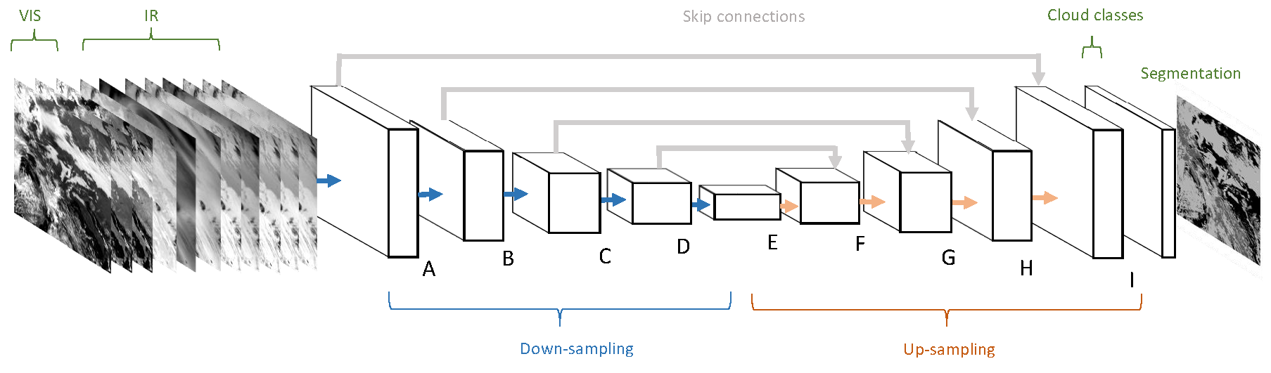
To train and evaluate CS-CNN, we use data from the Spinning Enhanced Visible and InfraRed Imager (SEVIRI) on Meteosat Second Generation (MSG) satellites. SEVIRI provides multispectral scenes with a temporal resolution of 15 [15], resulting in 96 scenes per day and 35,040 scenes per year. Because the data are available since the start of the MSG program in 2004, the training as well as the evaluation can be conducted with many data. Since it is not possible to perfectly label all these scenes manually, the well-validated Cloud Mask (CMa) from the CLAAS-2 dataset [21] were used as reference data in our work. This is, of course, a classification itself, but validation results show that it is very good. Additionally, noise in the training data is often used to prevent overfitting of the trained model [31]. Furthermore, for other segmentation tasks, generated reference data are beneficial, since they increased the number of training data [40]. Figure 1a shows an RGB-composite created from SEVIRI Channels 1–3 on the left and the CMa (b) on the right. In the example, large and small cloud areas as well as areas covered with snow (Northern Germany and the Alps) are evident. Above the North Sea, cloud fragments can be seen whose surroundings appear cloudless in the RGB image. In fact, there are cloud-contaminated pixels, as represented in the cloud mask. The combination of both datasets presents a perfect opportunity to evaluate the capabilities of CNNs with a segmentation architecture on a massive number of data for training, validation, and evaluation. Before the architecture of the CS-CNN is explained in depth, the used datasets and the connected challenges are introduced in more detail below.
3.1. MSG SEVIRI Data
The satellites of the MSG program provide images of a hemisphere (full-disc) covering the Atlantic, Europe, and Africa. Each scan produces a raster image with a size of 3712 × 3712 pixels and a resolution of at the sub-satellite point (SSP) at 0N, 0E. Its temporal resolution is 15 , which is the time for a full scan including required onboard processing. The eleven main channels of SEVIRI are centered at wavelengths ranging from to , as shown in Table 1. Additionally, a panchromatic channel, called HRV, covers multiple wavelengths [15].
A sub-region of the SEVIRI full-disc centered on Europe was selected as our study area. This enabled the evaluation of the influence of diurnal and seasonal as well as land/sea effects while focusing on a single image tile. It covers parts of the Atlantic in the west and continental areas in the east. In the north, it covers parts of Great Britain and Norway as well as the North and Baltic Seas, while the Mediterranean Sea is covered in the south. This area, therefore, includes land and sea as well as lowlands and mountains (Alps and the Pyrenees) that are often covered by snow.
As shown in Table 1, four channels are sensitive to reflected solar irradiation. The band/channel name coincides with the official naming for MSG-SEVIRI by EUMETSAT. The visible Channels (VIS) 1 and 2 as well as Channel 3 are dark at night, while Channel 4 covers both solar reflection and thermal emission during the day and only thermal emission during night. The other channels (Channels 5–11) measure surface emission in the mid and thermal infrared. At wavelengths of and , two channels cover the Water-Vapor (WV) absorption band of the atmosphere, and the channel at is sensitive to Ozone concentration [15]. SEVIRI raw data are provided by the European Organization for the Exploitation of Meteorological Satellites (EUMETSAT) and available from the EUMETSAT data portal. The available level 1.5 product is geolocated and corrected for all radiometric and geometric effects [41]. Since the MSG program started in 2004, the number of data continues to grow by approximately 8 B (compressed) per day. Since the raw data have variable offsets and do not correspond to a physical unit, all channels are normalized and transformed in a preprocessing step. However, the handling and transformation of 10 years of SEVIRI data, totalling about 23 TB (compressed), requires adequate tools. We used the data processing tool developed in our previous work [42] to transform the solar Channels 1–3 into reflectance values [43], to correct them to overhead sun and to transform the (IR) channels into radiance values [44].
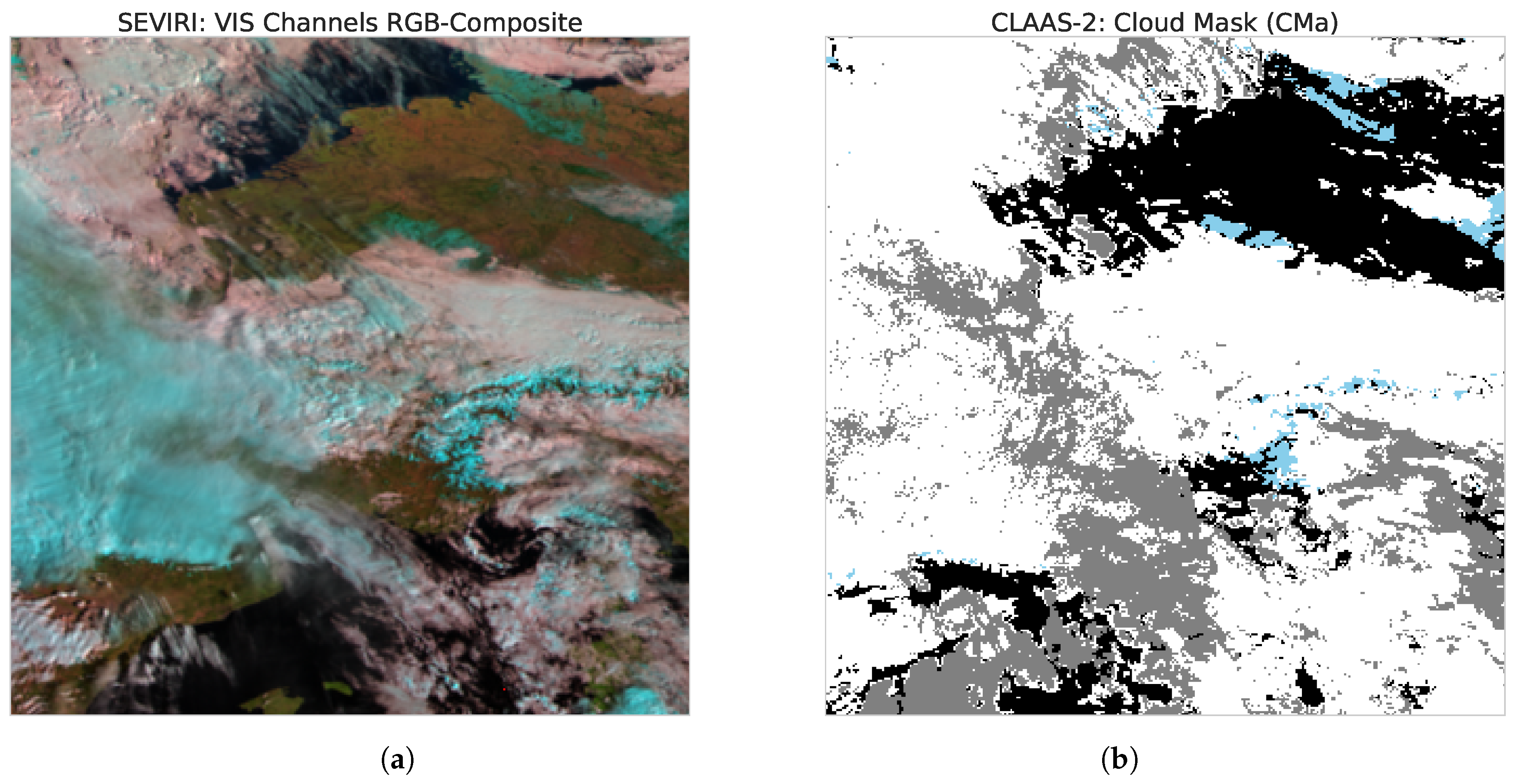
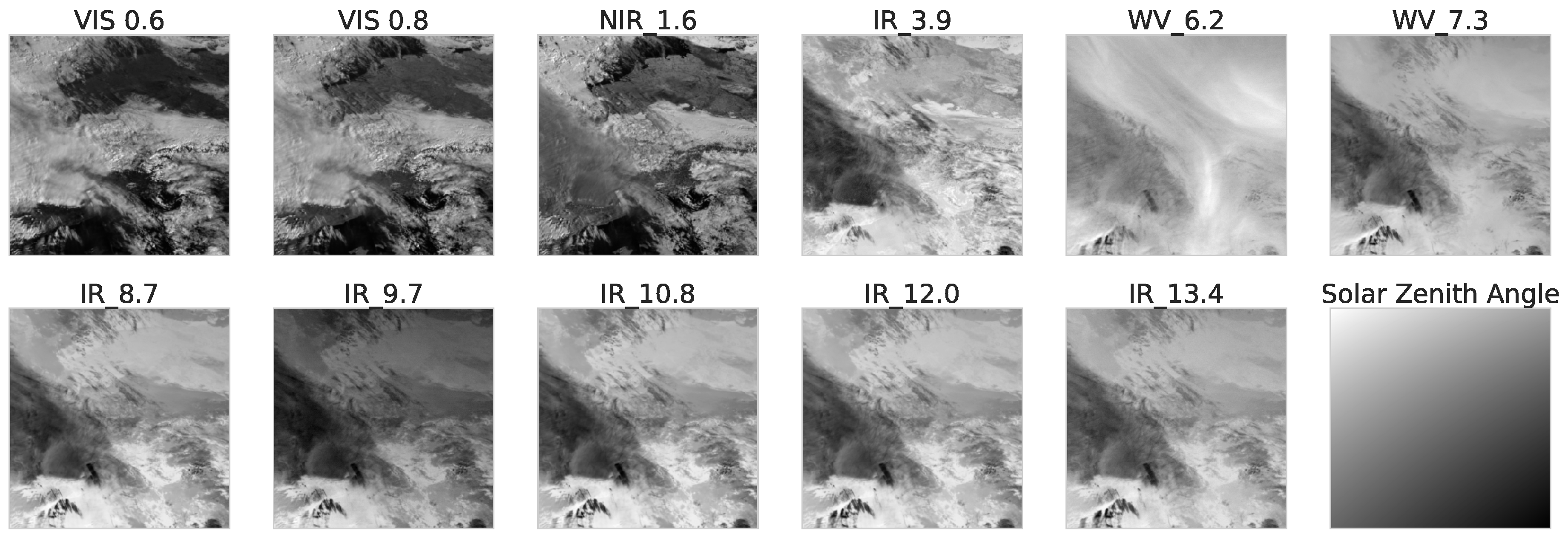
The geostationary position of the MSG satellites causes challenging effects in some of the 11 channels. These are mainly due to the satellite view angle and the solar zenith angle. The satellite view angle indicates the angle between the SSP and an observed pixel. It depends on the location of a pixel and increases with the distance to the SSP. This causes the edge of sensor pixels to grow up to a size of 11 over Europe. The same effect influences the distance between satellite and pixels. Therefore, the air column and thus the amount of absorbing gases such as CO also increases. Channels 1–3 pose additional challenges caused by the solar zenith angle. Obviously, these channels are dark at night and therefore do not provide information. At daytime, sunlight might get reflected by water surfaces causing glare (sunglint) effects. Channel 4 changes its characteristics depending on solar irradiation. While the IR signal is dominant at night, the reflection of solar irradiation is dominant at daytime. To handle these effects, classification approaches often require an input raster with the sun zenith angle for each pixel (Figure 2).
3.2. CLAAS-2 Cloud Mask
The CLAAS-2 dataset [21,45] provides different cloud properties derived from MSG SEVIRI data, including a cloud mask (CMa), cloud top height and cloud phase for the 12 years from 2004 to 2015. The algorithm used to generate the CMa data is a modified version of the SAFNWC-MSGv2012 algorithm [46] that is used for nowcasting by the Satellite Application Facility on Climate Monitoring (CM-SAF). While the algorithm was run on aggregated pixels for nowcasting to lower the required runtimes, it was applied for each pixel individually to create the CLAAS-2 dataset. The CMa provides a classification into four classes for each pixel of a SEVIRI scene [46]:
- Cloud-free: The pixel is not contamination by cloud or snow/ice.
- Cloud-contaminated: The pixel is partly cloudy (mixed) or filled by semitransparent clouds.
- Cloud-filled: The pixel is completely filled by opaque clouds.
- Snow/ice contaminated: The pixel contains snow or ice.
The CMa algorithm includes several threshold tests as well as spatial tests aggregating pixel neighborhoods that are applied to individual pixels. Pixels are first classified as cloud-contaminated using threshold values. If the value of a pixel is sufficiently distant from the threshold, it is also classified as cloud-filled. For each pixel, the confidence for the decided class is also present in the dataset. Moreover, the tests distinguish between conditions caused by solar irradiation (day, night, and twilight) as well as land and sea [46]. This allows using specific thresholds for effects such as sunglint over sea or the different properties of the channel at day and night.
Since the CMa is operationally used, validation studies are available for the CLAAS-2 dataset [21]: The validation study used data from active and passive instruments on low earth orbiters. The Cloud-Aerosol Lidar with Orthogonal Polarization (CALIOP) is an active instrument, while MODIS is a passive instrument. The study shows that the CLAAS-2 data, including the cloud mask, agree overall very well with the reference datasets and that no severe discrepancies were found. However, since the technologies of the reference platforms and SEVIRI differ significantly, no perfect pixel matching is possible. Additionally, there are known technical limitations that include classification of snow/ice contaminated pixels. Since the corresponding rules in the CMa algorithm require reflectance information from the solar Channels 1–3 to classify snow, the snow/ice class is only available for pixels with solar irradiation and therefore only at daytime [46].
3.3. Cloud Segmentation CNN (CS-CNN) Architecture
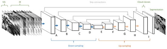
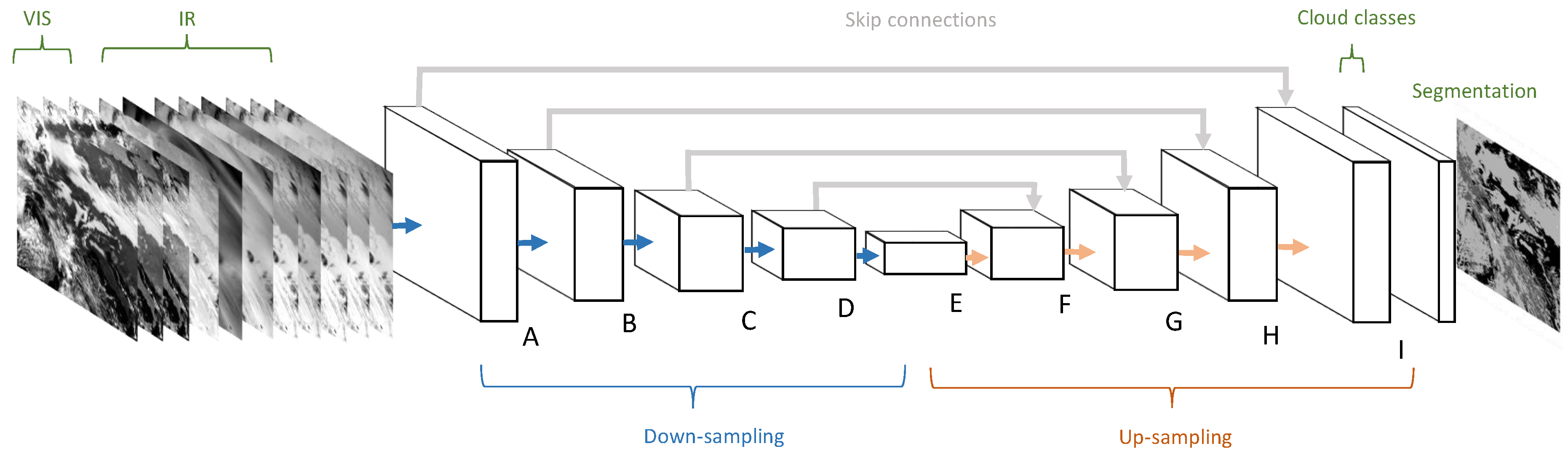
Due to its remarkable performance in biomedical image segmentation, we decided to use the U-Net architecture [12] as the technical platform for our CS-CNN, as illustrated in Figure 3. Its almost symmetrical architecture resembles several other CNN architectures for image segmentation [11,37,38] in terms of the composition of a sequence of down-sampling layers, followed by another sequence of up-sampling layers. We used the Caffe deep learning framework [47] to implement CS-CNN as a graph of connected convolution layers.
On the left hand side of Figure 3, the input for the network is shown. The spatial coverage is pixels, which matches the size of the selected study area. The depth of the input depends on the number of selected channels per scene. To evaluate the influence of the different channel characteristics, either seven or eight infrared channels (IR) and optionally the Channels 1–3 are used. The sequence of learning blocks, consisting of multiple convolution layers, is shown next to the input layer. Each block has a label (A–I) attached that refers to Table 2 where the details of the convolution layer blocks and their connections are given. The right hand side in Figure 3 depicts the computed cloud classes that return, for each pixel, the probabilities per class. Note that the output of the CS-CNN is a symmetric subset of the input with a size of only , since CS-CNN uses unpadded convolutions. For each of these pixels, the network outputs a five-dimensional probability vector that represents the degree of membership for each class. The meaning of the image right of the cloud classes differs when the CS-CNN is in the learning phase or in the application phase. In the learning phase, the image illustrates the reference data that are used to compare the CS-CNN result against to compute the loss for each training iteration. This information is then backpropagated through CS-CNN from right to left to adapt the weights of the different convolutional layers. In the application phase, the image represents the result of a trained model. For each pixel, CS-CNN assigns the class with the highest probability.
CS-CNN has similar principles as U-Net, but differs in some aspects. The architecture consists of blocks of convolutional layers that are listed in Table 2. In contrast to U-Net, the number of filters in each layer is much lower in CS-CNN to obtain a lighter network, and thus to improve the runtimes for classification. Each block in CS-CNN consists of two layers performing pixel convolutions with rectified linear unit (ReLU) as activation functions. In Blocks D and E, dropout is used to prevent over-fitting. Down-sampling happens as the last operation in Blocks A–D. In contrast to the U-Net, we performed down-sampling by strided convolutional layers instead of pooling layers. Strided convolutions are common convolution operations but they use a larger pixel stride. This enables the CNN to learn a specific down-sampling operation for each layer. To generate a segmented image, the down-sampling sequence is followed by up-sampling. The last layers in Blocks E–I in Figure 3 perform up-sampling by transposed convolutions (deconv). Moreover, CS-CNN also utilize features from down-sampling layers again in the corresponding up-sampling counterparts. These so-called skip connections have become an indispensable component in a variety of deep neural architectures.
A further difference between CS-CNN and U-Net is that CS-CNN does not require data augmentation, such as elastic deformations, to increase the amount of training data. Augmentations are beneficial when the training dataset is small. This is, however, not necessary in our cloud segmentation study, because many annotated raw satellite images (23 TB) are available by combining the SEVIRI and CLAAS-2 data. These large datasets are difficult to manage on commodity hardware, but our experiments show that additional data constantly improves the model accuracy.
4. Evaluation/Experimental Setup
In this section, we present the evaluation data, the experimental setup, and the methods to measure the performance of CS-CNN. CS-CNN was trained on three different input channel configurations that were selected to evaluate the influence of channels sensitive to solar irradiation. To compare CS-CNN against a classifier for individual pixels, we additionally trained two random forest models that we also describe briefly below.
4.1. Model Training
CS-CNN training was performed for three scenarios that contain increasing levels of solar influenced channels. This setup was selected to evaluate the necessity and impact of solar channels on the segmentation. All data from SEVIRI and CLAAS-2 generated between 2004 and 2010, i.e., a total of six years, were selected as the training data for all models. Since MSG and CMa are generated in 15-min intervals, this results in approximately 205,000 scenes. After removing all corrupted data, a total of 200,000 scenes remained for training. A scene was removed if either an MSG channel or the CMa was corrupt. The remaining scenes were randomly inserted in a list that was used for training.
Scenario A contains all 11 channels including Channels 1–3 that are dark at night. Recall that each training iteration consists of one scene with all 11 channels and the corresponding CLAAS-2 cloud mask representing the “truth”. While CS-CNN can handle dark areas without changes, glare effects in the reflectance Channels 1–3 can disturb the training process. We found that spiking loss (or error) values occurred during training when specific night scenes were ingested. This is because glare effects occur at night when the affected pixel should be dark. For certain sun angles, light either directly reaches the sensor or is reflected by the surface, while the other pixels of the scene are dark. For the study area covering Europe, this is especially true in the summer months. To solve this issue, we added a preprocessing step that masks a channel as completely dark when a glare effect occurs.
Scenario B includes thermal Channels 5–11 and Channel 4 that is dominated by the solar signal during daytime and the thermal signal at night. This reduces the influence of changing characteristics caused by the transition between day and night that CS-CNN needs to handle. Note that reducing the number of input channels does not create other changes in CS-CNN.
In Scenario C, only Channels 5–11 that are not directly influenced by solar irradiation are used for training. Thus, the channel characteristics will not change between day and night. Therefore, this scenario is expected to be the easiest to train.
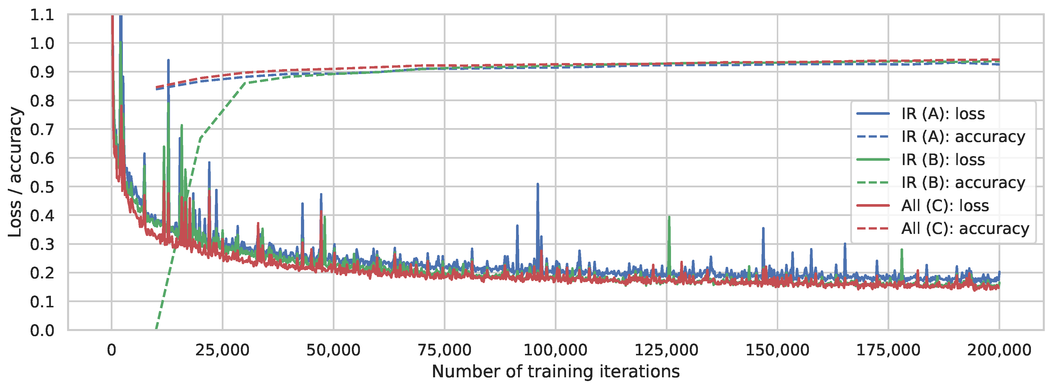
The training of all three scenarios was performed with an NVidia GeForce GTX TITAN X GPU. We selected Adaptive Moment Estimation (ADAM) [48] as our optimization method, since it provides excellent results and fast convergence. This is beneficial, since the training with all available scenes takes approximately 34 h. To validate the models during and after training, we used data from 2012, which contains 35,040 scenes. A random sample of 1200 scenes from 2012 was selected for this task. Figure 4 shows the training loss and the accuracy measured while training all model scenarios. The loss of all three scenarios drops rapidly until it is below 0.3, then it keeps decreasing with an increasing number of training iterations. At the same time, the accuracy of each scenario keeps increasing. After 30,000 iterations, equal to the number of scenes produced per year, the accuracy of Scenarios B and C approaches 90%, while Scenario A is already above 90%. Overall, Scenario A shows the highest accuracy and the lowest loss, but only with a small margin.
4.2. Evaluation Data
To evaluate and compare the performance of the models, we randomly selected 8000 scenes from 2011. The training data include only scenes for 2004–2010, which implies a total independence of the evaluation data and the training data. After removing corrupted scenes, a total of 7977, 23% of the 35,040 scenes created per year were used for evaluation and comparison.
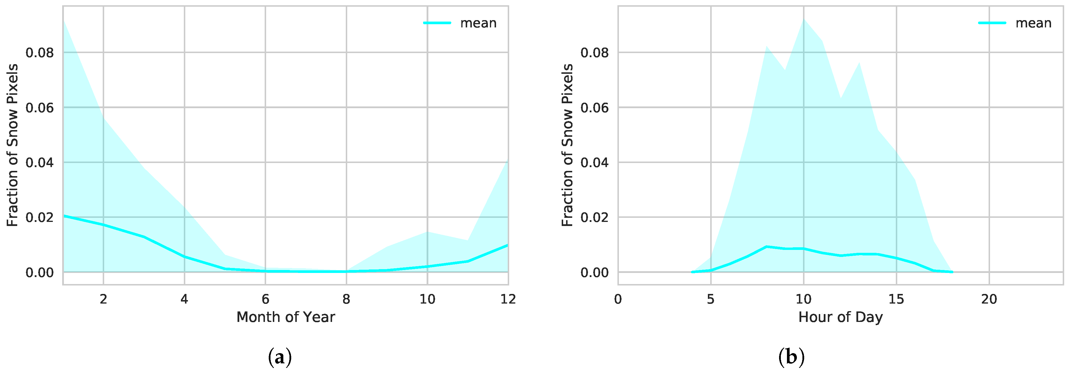
One of the challenges for cloud detection is the treatment of snow. While cloud and cloud-free pixels are equally distributed over scenes, the snow class is limited to daytime in the CLAAS-2 CMa scenes. Additionally, the occurrence of snow pixels in the study area is tied to seasonality. Figure 5 shows the variance as well as the mean snow fraction per scene aggregated by month of the year (a) and hour of the day (b). High fractions of snow pixels only occur during the winter months on the northern hemisphere where the maximum fraction per scene is 9.2%. In the summer months, the maximum and the mean fraction of snow pixels per scene fall below 0.05%. The right plot shows the dependency on sunlight for snow pixel information in the CMa product. Note that snow pixels are not available for night hours. During day, snow pixels mostly occur between 08:00 and 13:00, i.e., when there is a lot of sunlight. The maximum fraction of snow pixels is 9.2%.
4.3. Random Forest
We decided to use a random forest (RF) introduced by Breiman [49] as a competitor of CS-CNN in our comparison. RF classifies individual pixels and creates a classification by applying the model to each pixel. Recently, RF has been shown to perform very well for classifying multispectral satellite data [8,26]. RF is an ensemble learning method combining a large number of standard decision trees. In an RF model, each tree is trained separately by taking a bootstrap sample from the training dataset. The trees are built by splitting a random subset of the original input features at each node. The data are split in such a way that within each subset a chosen error function is minimal. This procedure is recursively repeated until the complete training dataset has been processed. An RF is straightforward to use and can easily handle vast numbers of input features and supports large datasets due to its sampling approach. The RF model used in this study is implemented in the Scikit-learn package for Python provided by Pedregosa et al. [50].
Equivalent to CS-CNN training, the same set and order of training scenes were used to generate two scenarios: In Scenario D, all 11 SEVIRI channels are used as independent input features to train the model. However, when used for multispectral classification, RF methods often use auxiliary data such as terrain elevation, the satellite viewing angle, and handcrafted geo-statistical texture features [8]. Therefore, we examined a second RF scenario (Scenario E) where additional features are introduced. These are combined channels (differences) as well as geo-statistical texture features. Note that these geo-statistical features provide information about spatial structure in the SEVIRI data. Afterwards, a recursive feature elimination was conducted to select the most relevant features, as reported in Table 3.
4.4. Evaluation Metrics
The evaluation metrics are based on the comparison of the CMa data with the results of the trained model scenarios. For each scene of the evaluation data, the classification generated by a model is compared pixel by pixel with the CLAAS-2 cloud mask, and the results are represented as confusion matrices for each class as well as combined (overall). A confusion matrix contains four counters to track the true positive classified pixels (correctly predicted events), the false positive (incorrectly predicted events), the true negative (correctly predicted no-events) and the false negative ones (incorrectly predicted no-events). For each scene independently, local confusion matrices are generated to compare individual scenes and analyze the distribution of the evaluation metrics over time. Additionally, the local confusion matrices are combined into global confusion matrices that cover all scenes and represent 837,393,552 classified pixels in total. This is the foundation to calculate the following indicators for the performance of each model. First, the accuracy of a class is the portion of positive and negative pixels classified correctly. Second, Probability of Detection (POD) returns the portion of pixels that correctly belong to a class. Third, Probability of False Detection (POFD) gives the relative amount of pixels falsely classified. Fourth, False Alarm Ratio (FAR) provides the probability of a false classification if a pixel is classified as belonging to a class. The metrics are described in detail by Jolliffe and Stephenson [51] and are also used by similar studies (e.g., [8,26,52]).
The described metrics are used to evaluate the performance of each model. In addition to the accuracy of each class, which measures the proportion of correctly (positively or negatively) classified pixels, we calculated POD that indicates the proportion of pixels that correctly belong to a class. Information on errors is provided by POFD, the ratio of false classifications and the number of all pixels, and FAR indicating the proportion of pixels that a model has classified as belonging to a class where this is false. The bias provides information whether a model overestimates or underestimates a class, i.e., optimally the bias is 1.0. To determine the skill of the models, we calculated the HSS. The HSS reflects discrimination and reliability and measures the improvement compared to a (random) standard classification.
5. Evaluation Results
The goal of this section is to report our experimental results of the different scenarios introduced in Section 4.1 and Section 4.3. First, we show an example classification for a single scene using both classification approaches, the CS-CNN and the RF method. Then, we compare the global statistics of all three deep learning scenarios (Scenarios A–C) and the two RF scenarios (Scenarios D and E). The robustness of the different models is investigated by comparing the distribution and variance of the classifications of all individual scenes. Additionally, we investigate the impact of seasonality and the time of day on the models. Finally, we show the influence of pixels located close to the spatial boundaries of cloud entities.
5.1. Example Scene and Performance
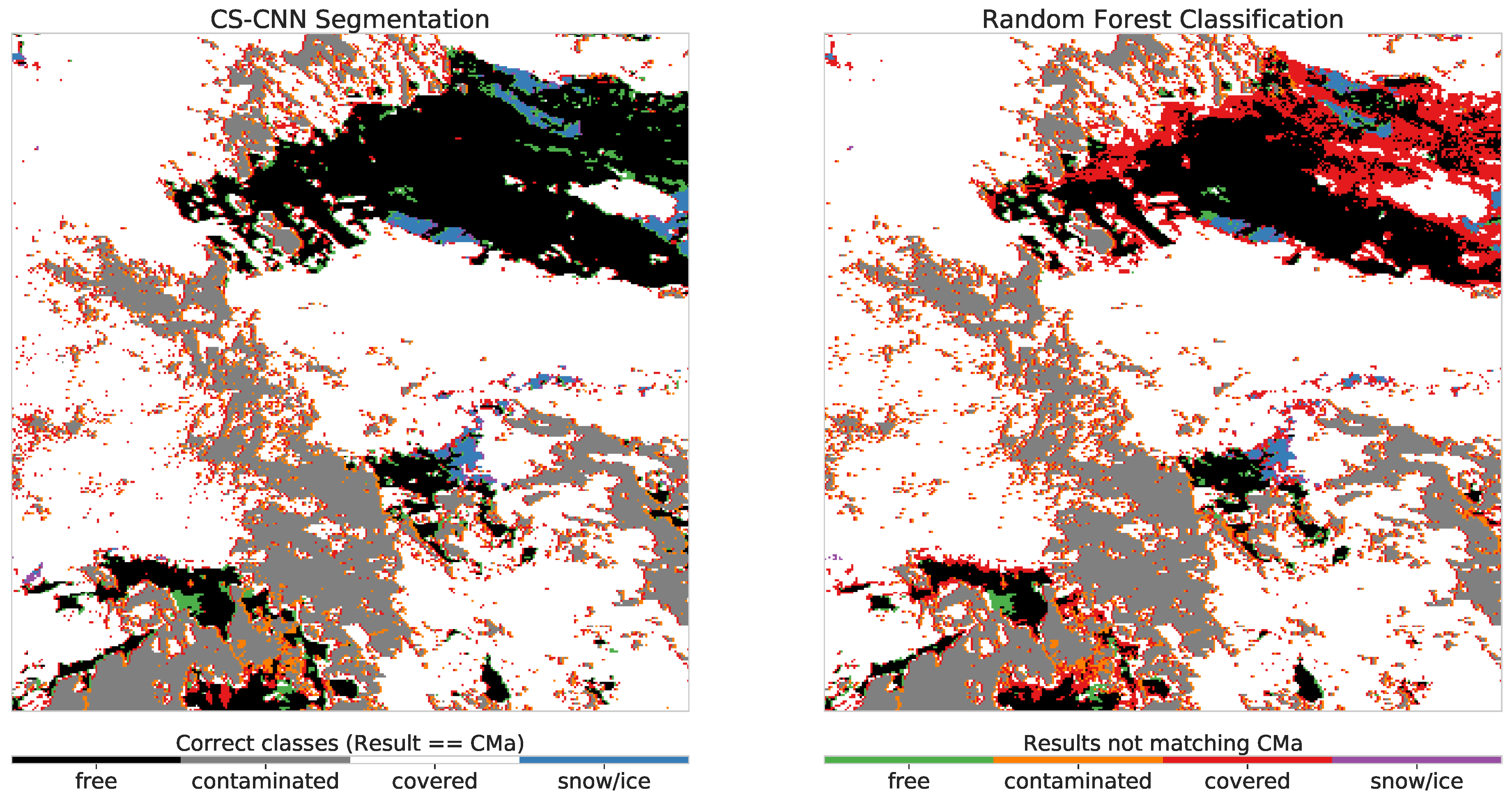
The scene introduced in Section 3 was also selected to present a first example of the CS-CNN and the random forest classification. Figure 6 shows the cloud mask of CS-CNN and RF on the left hand side and right hand side, respectively. The RGB composite of the SEVIRI Channels 1–3 as well as the CLAAS-2 cloud mask of this scene are depicted in Figure 1. Again, the four classes (cloud-free, cloud-contaminated, cloud-filled and snow/ice) are visualized. Additionally, we added a different colorization for pixels where the class selected by the model does not match the original class in the CMa.
Confusion matrices were calculated by comparing the model results with the original cloud mask pixel by pixel. Table 4a,b represent the result for the example scene (22 February 2011 09:00:00 UTC). By looking at both results, one can already reasonably conclude that CS-CNN provides results close to the original. The RF results also show that cloud areas are correctly classified in general. However, larger contiguous misclassified areas are recognizable in the northeast. This is confirmed by the statistics in Table 4a,b, where the overall skill is 0.905 for the CS-CNN while the RF archives a skill of 0.885. While both results deviate slightly from the original, the CS-CNN shows differences to the original model only at spatial boundaries of entities. The RF classification shows many differences at the north-eastern corner, where a large cloud-free area is classified as clouded. These areas in northern Germany are bright, probably sandy, ground pixels and in the northwest pixels corresponding to the coastline. Both are common problems [16,18] that can occur when classifying clouds.
The statistics agree with that observation and show a cloud-free skill of 0.920 for the CS-CNN and 0.865 for the RF model. In the same area, the RF model also underestimates snow patches, which correlates with the skill for snow classification. It is 0.668, while the CS-CNN has a skill of 0.824. The confusion matrices generated for both models show that undetected snow pixels are equally classified by CS-CNN as cloud-free (257 of 595) and cloud-filled (314 of 595), while RF assigns most of them as cloud-filled (754 of 945).
Both approaches were run on a machine with Intel i7-5930K CPU (3.5GHz), 64 GB RAM, and an NVidia GeForce GTX TITAN X GPU. Data loading is implemented equally for all methods and the loading time is excluded from the execution times stated in the following. Caffe can run CS-CNN (A) on CPU and on GPU. The execution time on the CPU for CS-CNN is while a run on the GPU takes only 25 on average.
The application of the RF model (E) to all pixels of a scene takes on average. The implementation uses the Scikit-learn library and runs on the CPU. It uses all 12 CPU cores for RF training and application. The RF scenario requires the generation of spatial features and channel combinations for each scene, which takes and is included in the runtime. While GPU based RF implementations are also available (e.g., [53]), the Scikit-learn results allow a comparison of the accuracy of the technologies. Additionally, the overhead for feature generation and channel combinations is independent of the RF implementation.
5.2. Global Results
To evaluate the performance and to compare the trained CS-CNN models with the RF models, the global statistics of all classes are presented in Table 5a–e. For this part of the evaluation, the results from all test scenes were combined to generate global confusion matrices. Therefore, the presented tables show the results calculated using all pixels considered in the evaluation.
Table 5a shows the results for the cloud-free class. CS-CNN Scenario A, trained with all channels, dominates all metrics except POD and bias, while Scenario C, trained without solar channels, shows the highest POD, it has higher FAR and POFD values. Scenario D, the RF trained with all channels, shows the smallest bias, but the other values are not as good as in the CS-CNN scenarios. The accuracy and HSS values of RF Scenario E are smaller than the CS-CNN values, and the error values are smaller than the error values of Scenarios A and B.
The metrics for the cloud-contaminated class are shown in Table 5b. RF Scenario E shows the best values for this class. This scenario is also the only scenario that overestimates this class, as indicated by the bias. Additionally, the other RF scenario (Scenario D) shows values clearly below the values of the CS-CNN scenarios. The CS-CNN metrics show the best accuracy and skill values for all channels (Scenario A), and the lowest error values are achieved for the scenario without solar influenced channels (Scenario C).
Table 5c shows the metrics for the cloud-filled class. Here, CS-CNN Scenario A again shows the highest accuracy, skill, and POD values. CS-CNN trained without the reflectance channels (Channels 1–3) shows the lowest error values. Both RF scenarios (Scenarios D and E) have higher error values than any CS-CNN scenario. Scenario D clearly shows the lowest accuracy and skill, Scenario E shows the second best.
The snow class results are presented in Table 5d. Here, the accuracy values are very high for all scenarios, which is related to the small fraction of snow pixels per scene, as indicated by Figure 5. The HSS of CS-CNN Scenario A (0.882) is the only one exceeding 80%. The POD is also clearly dominated by the CS-CNN scenarios, while both RF scenarios are below 70%. The FAR values are high for CS-CNN without solar channels and lowest for RF scenarios, while the POFD is very low for all scenarios.
The accuracy and the HSS for all classes combined are presented in Table 5e. For both metrics, CS-CNN Scenario A shows the highest values. The scenario with the second best values is CS-CNN Scenario B with a very small difference separating it from RF Scenario E. While the CS-CNN without solar channels is very close to the other ones, the RF Scenario D shows the lowest values with a clear difference to the next best scenario.
5.3. Robustness
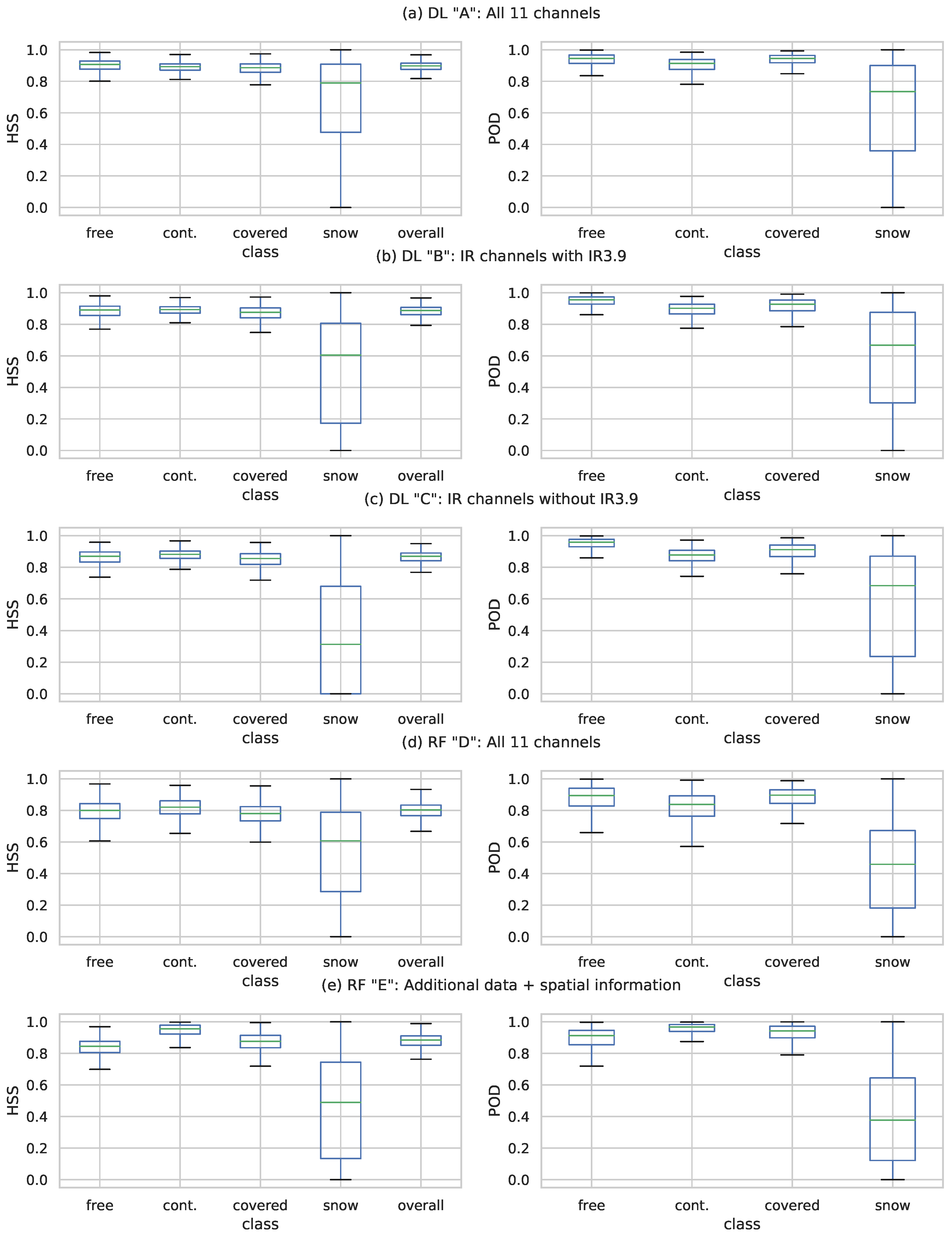
For a robust model, values such as accuracy and skill (HSS) should have a high median value and a small range for each class over individual scenes. Additionally, different classes should also be at a similar accuracy and skill levels to keep the overall skill level even if distributions of pixels per class changes. Figure 7 shows the box-plots of HSS and POD for all five models in the same order as the tables in the previous section. Here, the box-plots are created from the individual results of each of the 7977 evaluation scenes. The box represents the second and third quartile, containing 50% of the scenes, while the median is represented as the (green) dividing line. For a robust model, i.e., a model that produces reliable results and a constant quality level, we expect small boxes. This means that the HSS values of a class are, in the optimal case, not changing between scenes with different class distribution. Additionally, the whiskers, representing the overall data distribution, should cover only a small area so that there is no extreme difference between high and low values.
The first row in Figure 7 represents CS-CNN Scenario A. The left plot shows the HSS, the right plot shows the POD generated from all 7977 scenes. For HSS, almost identical median values and value ranges are displayed for the cloud-free and cloud classes as well as for all classes combined. The snow class shows a HSS median value of 0.8, and the second and third quartiles cover a range from 0.5 to 0.9.
CS-CNN Scenario B is shown Figure 7b, indicating the impact of removing Channels 1–3. Most classes show a pattern similar to Scenario C, with slightly lower values. Similar to the global results in the previous section, the values of the ice/snow ice class show the largest changes. The value ranges of HSS and POD shift down and grow. Most notably, the HSS medium value for snow/ice is now 0.6.
CS-CNN Scenario C, represented by Figure 7c, again shows patterns similar to the previous two scenarios. Cloud and cloud-free classes have slightly lower values compared to Scenario B, which is also true for all classes combined Again, the ice/snow class deviates significantly from the other classes. Here, the median of the HSS is 0.3, while the POD shows a median similar to Scenario B.
Comparing the RF Scenario D, which uses all SEVIRI channels, with the equivalent CS-CNN Scenario A, it can be seen that the overall HSS and the overall distribution are considerably lower and cover larger ranges. The median for the cloud classes and overall show a uniform level near 0.8, while the HSS for ice/snow is at 0.6. The POD for all CS-CNN scenarios have a nearly identical pattern, which can also be seen for this RF model, albeit with significantly lower values and larger value ranges.
RF Scenario E, which uses all SEVIRI channels, auxiliary data, and spatial statistics, improves all metrics except for snow when compared with the previous RF model. When compared with the CS-CNN Scenario A, it is visible that the HSS median and the second and third quartile box for most classes show value ranges at a lower level. The exception is the cloud-contaminated class that shows a very high median value and a small box between 0.9 and 1.0. Compared to the previous RF model, the HSS values for snow/ice are lower, which can also be seen on the POD plot.
5.4. Seasonal and Diurnal Dependencies
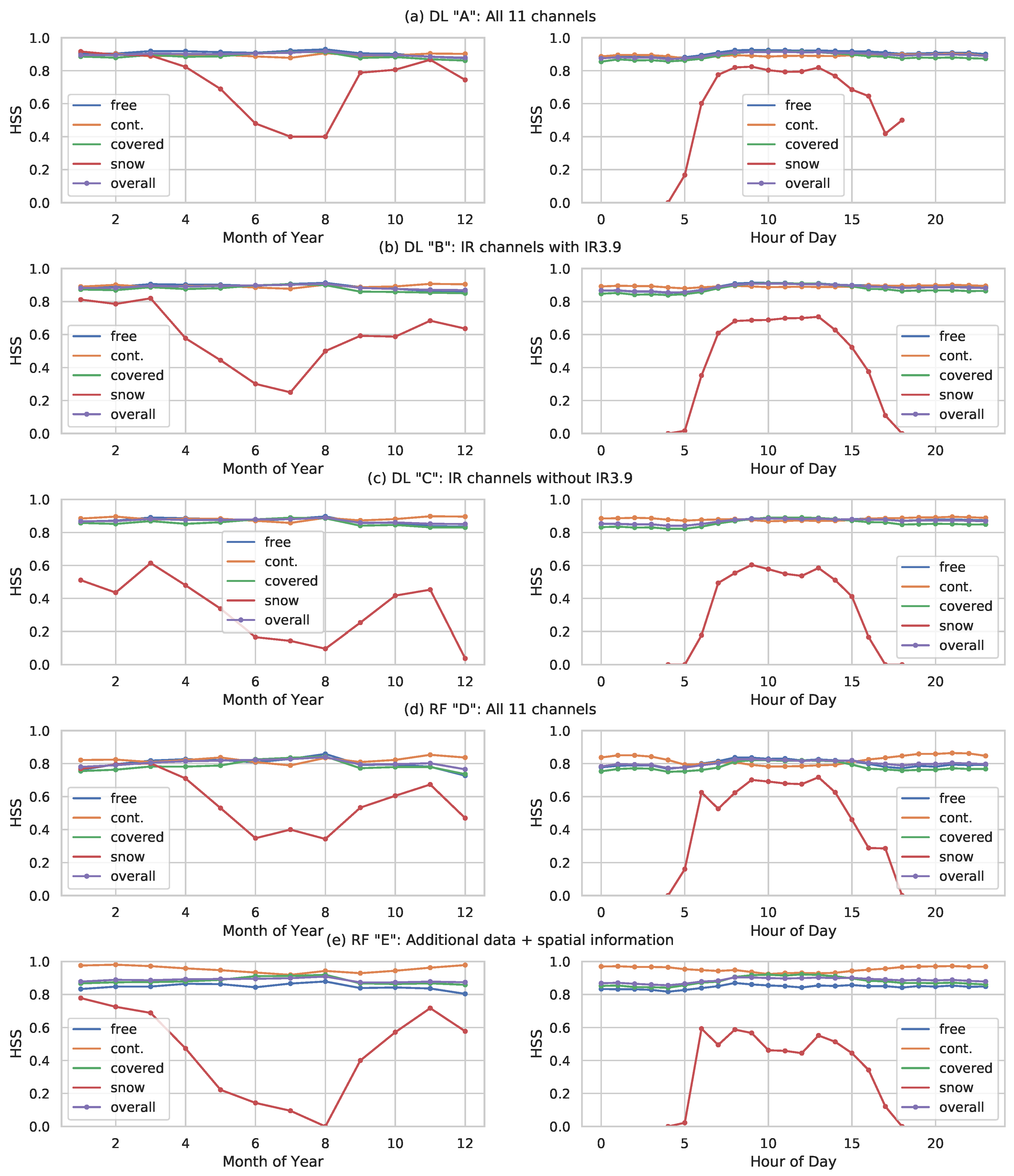
The snow class in the CMa data depends on seasonality, since there is less snow in Europe in the summer months. Additionally, the CMa algorithm uses the reflectance information from solar Channels 1–3 to classify pixels as snow covered. Therefore, there are no snow pixels in the CMa data at night [46]. The influence of this aspect requires further investigation. Figure 8 shows the HSS values grouped and aggregated by month of the year on the left side and by hour of the day on the right side.
For all CS-CNN scenarios, the seasonal variation of the cloud classes and the combined classes is quite low. All classes show values between 0.8 and 1.0, which are constant over the year, where Scenario A shows the highest values. However, the snow/ice class reaches a HSS level of 0.9 during winter months, which is at the skill level of the other classes, but drops to 0.4 during the summer months. A dependency on the hour of the day is also clearly shown by the right plot. In the night hours, no HSS is shown for snow/ice pixels while it rapidly rises (and falls) with solar irradiation between 5 am and 6 pm to a level of 0.8.
Similar to the previous results, CS-CNN Scenarios B and C show slightly lower HSS values for all classes. While the HSS of the cloud classes and overall remains at a high level, significant changes are visible for the snow/ice class. Scenario B shows lower HSS and POD values, and Scenario C shows that the HSS level during summer months drops to 0.1.
The RF Scenario D show seasonality patterns similar to the previous CS-CNN scenarios, but at lower value range. For all classes and overall, relatively constant HSS values between 0.7 and 0.9 are visible, with the exception of the snow/ice class. For this class, a comparable skill is shown during the winter months. However, it drops to to 0.4 during summer, similar to CS-CNN Scenario A. The diurnal distribution of performance shows a similar pattern. At night no skill for snow/ice is displayed, with solar irradiation, the skill rises up to 0.7 and varies over the day. The patterns for the RF Scenario E show the most significant seasonal and diurnal dependencies, while still resembling the ones shown by the other scenarios. In contrast to the other models, this one shows clearly visible differences for all classes for daytime and month of the year. Cloud classes stay between an HSS of 0.8 and 1.0, however, they show more deviating value levels. The snow/ice class again shows different patterns. While the performance in the winter months is similar to the other RF model, the performance drops to a value near 0.0 during summer. The diurnal distribution shows similar patterns but snow/ice stays below an HSS of 0.6 during daytime.
5.5. Impact of Entity Boundaries
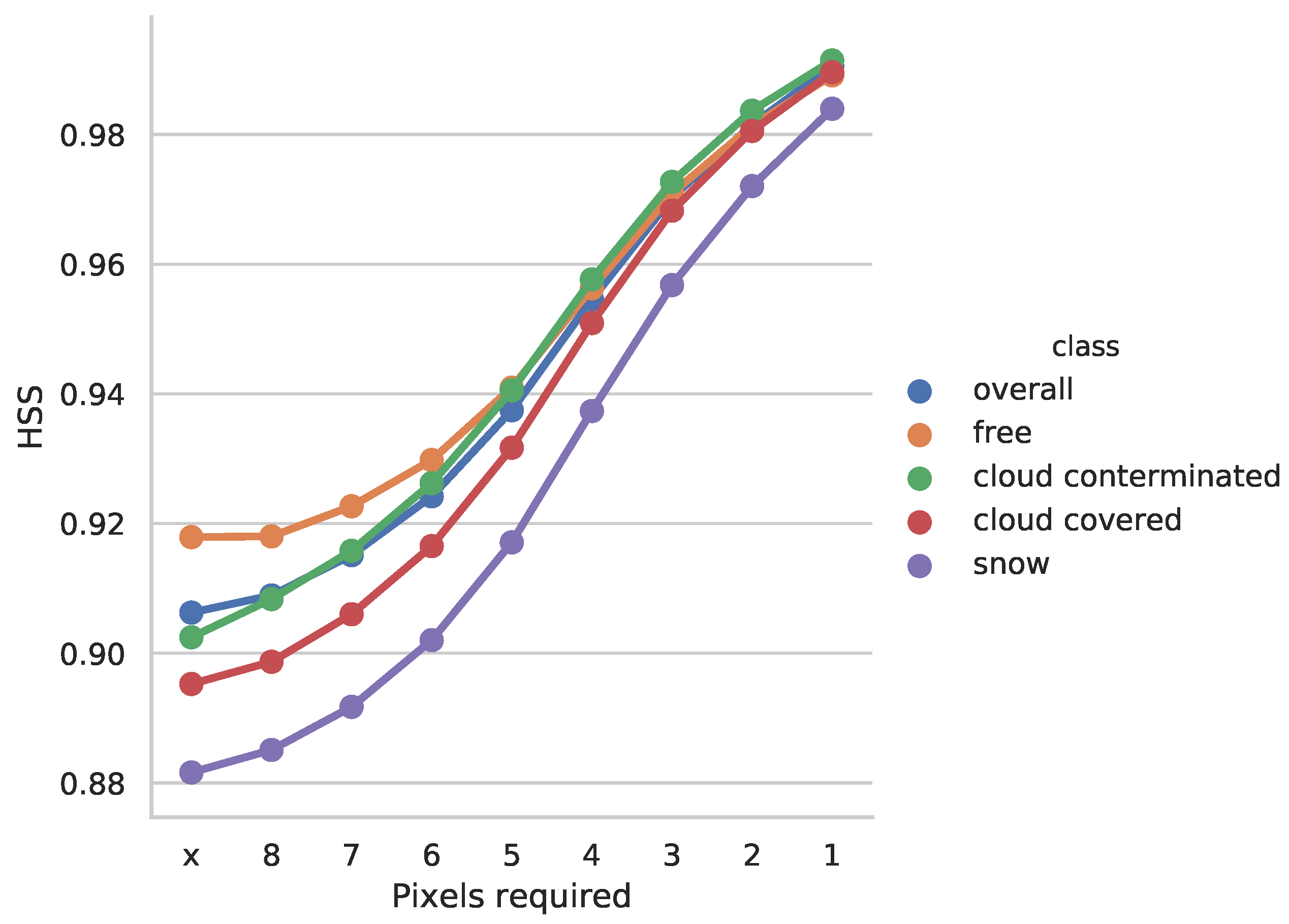
As shown in Figure 6, the CS-CNN segmentation shows deviations from the original cloud mask almost exclusively at cloud or snow entity boundaries (or edges). The RF classification in the same figure also shows a similar pattern, but there are also larger areas that do not match the CLAAS-2 cloud mask. To determine the actual effect of this error type, the evaluation of the results was modified in such a way that deviating pixels at entity boundaries are selectively excluded. Pixels at a boundary have at least one adjacent pixel with a different class. Now, we adapt the evaluation in such a way that we do not count pixels as wrong if there is at least a certain number of neighbors in the original cloud mask with the same class. If all eight neighbors of a pixel have the same class in the CMa, but the pixel class deviates from the CMa, it could be considered noise. In the other cases, it can be assumed that the pixel is at the edge of an entity.
For the range of 8 to 1 required correct adjacent pixels, the evaluation was executed again for CS-CNN Scenario C. Figure 9 shows the resulting HSS values for the range of required correct neighbors. Reducing noise already shows an influence on the performance metrics of the segmentation. Excluding the pixels at entity boundaries from the evaluation clearly shows that the HSS increases above 98% for all classes. Even if only those pixels are excluded that have at least four neighbors with the same class in the original cloud mask, a significantly better result is already achieved.
6. Discussion
In this section, we discuss how CS-CNN copes with several issues compared to previous approaches for cloud classification.
The first issue of previous methods is their poor usage of spatial information. This is different for CS-CNN, since it is based on U-NET, an architecture for image segmentation, as described in Section 3.3. Similar to U-Net, CS-CNN uses convolutional layers and learns to classify the multispectral SEVIRI data from spatial structures on multiple resolutions. Our results, presented in Section 5, show that CS-CNN produces excellent classifications with an overall HSS above 90% and accuracy levels above 94%. Looking back at the results of the specific models, clear patterns emerge. First, it is obvious that using solar reflectance Channels 1–3 improves the results of the CS-CNN. While the cloud classes show very good results in all scenarios and continue to improve with an increasing number of scenes for learning, the snow class is particularly striking. However, it should also be noted that the results for scenarios that do not include Channels 1–3, already show good POD values for the snow class. Confusion matrices generated over all scenes for CS-CNN (A) and RF (E) contain the distribution of undetected snow pixels, which is similar to the example scene. CS-CNN assigns them equally as cloud-free (45%) and cloud-filled (51%) while RF assigns the majority (67%) of them as cloud-filled. A look at the robustness of the models shows that the CS-CNN model using Channels 5–11 is already very robust. The skill of all classes is improved by adding solar channels, but only the snow class changes significantly. Therefore, we conclude that the IR channels alone are sufficient to generate robust cloud masks where the skill of each class is at the same level and has a small value range, as described in Section 5.3.
As discussed in Section 1 and Section 2, threshold-based and machine learning approaches require expert knowledge to identify relevant rules and features by hand. Productive cloud masks such as CLAAS-2 CMa use many rules to handle different characteristics of multispectral data where various parameters such as the position of the sun play a role in the classification. The random forest used in our study learns a classification of cloud pixels from the multispectral SEVIRI data. However, as shown in Section 5, it is not sufficient to use the satellite data alone. The first RF model shows lower HSS and POD values than the CS-CNN models. Only by adding additional data, handcrafted spatial information, and channel combinations, an RF model could be generated that comes close to the results of CS-CNN. This is not necessary when using CS-CNN, because CNNs learn the spatial features inherently. Moreover, in terms of robustness, we observed another strength of the CS-CNN models. The CS-CNN models provide very homogeneous classifications for all classes. This is different for the most advanced RF model. Although the feature selection for the model has led to improvements for the cloud classes, it considerably worsened the results of the snow class. This clearly shows that the use of the CS-CNN is considerably more robust than RF since the cloud and cloud-free classes show similar HSS values with small variability. Additionally, SC-CNN is not sensitive to common classification problems such as bright surface pixels (sand) and coast lines. Moreover, the application of traditional learning methods such as RF requires considerably more expert knowledge in terms of handcrafted features and feature selection.
The third issue is the need to support nowcasting and processing of large time series with respect to low latency and fast processing, respectively. Deep learning frameworks, such as Caffe, speed up CNN execution by implementing the different layers for execution on GPUs. Thus, the runtime required to classify a single scene is very short (within milliseconds), as shown in Section 5. The proposed CS-CNN classifies an input scene instantly (25 ms) on a GPU. Execution on a CPU requires a significantly longer time (1.24 s) and the classification using RF takes which includes the time to generate spatial information and combine channels.
In the following, we look at the special aspects and challenges of CNNs for cloud detection and multipectral data. A great effort was the preparation of the training and evaluation data, which in this case was the pre-processing of 23 TB of compressed raw data into tiles and the transformation of raw values into physical values. Here, we see a considerable need for improvements, which would also be beneficial for other approaches. For example, it would be a great advantage to describe pre-processing as a reusable and portable workflow. This would be similar to the design of CNNs in Caffe, which are described textually as a graph of operations. This would make re-application, adaptation to other data, and parameter changes much easier.
Despite its excellent performance, one of the important requirements of CS-CNN is the availability of ground truth information for the learning phase and the performance evaluation. In particular, a public dataset with only correct labels of clouds is not available yet. Additionally, labeling the amount of data used for this study manually is infeasible. We circumvented the problem by using a well validated dataset, CLAAS-2 CMa, as reference data for CS-CNN. Note that CLAAS-2 CMa suffers equally from the challenges presented in Section 3 for the SEVIRI data. Our study also shows that a large amount of training data constantly improves the accuracy of the model. However, it can be seen in Section 4.1 from the training progress that even small amounts can produce accurate models. This can be complemented by technologies for data augmentation as used by U-Net [12]. Data augmentation generates additional training data, e.g., through distortions or rotations of the available data.
An interesting aspect is whether the use of a different classification technique can identify relationships that are not explicitly specified. We used CLAAS-2 CMa for training, which uses threshold-based methods. These require the VIS channels to detect snow in the SEVIRI data. We know that the performance of CS-CNN for the snow class depends on the time of day, as shown in Section 4.2. As expected, CS-CNN can detect the snow class better if the solar channels are included. However, this only means that the CNN can resemble the CLAAS-2 CMa better and not that the classification of the real snow cover is actually more correct. Obviously, CS-CNN is able to learn correlations that are only implicit in the original. This is evident from the fact that the snow areas can be well classified from IR data alone. The median FAR values for the snow class of the IR only CS-CNN models are 45% and 36%. However, the CLAAS-2 CMa does not contain snow in night scenes, so even a correct detection of snow would be considered wrong and increase the FAR in these cases. We have observed scenes in which CS-CNN has detected obvious snow areas even if they were not included in the original. It is therefore possible that the CS-CNN classification can perform some aspects better than the original. For a more detailed investigation, however, real ground truth data are required.
There are several objectives for future work. For example, we need to generate real ground truth data, which often are not available for remote sensing tasks. This is especially relevant for snow, where pixels in night scenes could be considered as snow if the day scenes before and after had snow. Furthermore, the very good results obtained by the presented CS-CNN suggest to apply CS-CNN to similar challenges. For example, classification of individual cloud types, detection of precipitation areas, and estimation of rainfall will be examined in our future work. Therefore, additional input data such as cloud top pressure or model data should be examined. Future work could also enhance e-research systems/labs such as the VAT system [54] to combine CNN training and execution with workflow-based data handling, preprocessing, and visualization of results.
7. Conclusions
In this paper, we present CS-CNN, a novel cloud mask generation approach using a CNN with a segmentation architecture. We show that the architecture of CS-CNN is very well-suited to process multispectral remote sensing data and to classify clouds. Compared with a frequently used random forest approach, CS-CNN requires significantly less expert knowledge and effort. Compared with the random forest approach, the results of CS-CNN show higher accuracy, are produced faster, and are significantly more robust, i.e., they are more consistent. CS-CNN provides high overall accuracy (0.94) and HSS (0.90) values and requires only 25 ms of computation time for classifying an input scene.
Author Contributions
Conceptualization, J.D., N.K., M.M. and B.T.; Data curation, J.D. and S.E.; Funding acquisition, J.B., B.F. and B.S.; Investigation, J.D., N.K., S.E. and B.T.; Methodology, J.D., N.K., M.M. and B.T.; Resources, S.E., M.M. and B.T.; Software, J.D., N.K. and S.E.; Visualization, J.D.; Writing—original draft, J.D. and B.S.; and Writing—review and editing, J.B., B.F. and B.S.
Funding
This work was financially supported by the German Science Foundation (DFG) grant numbers BE1780/40-1, FR-791/15-1, SE-553/7-2 and TH1531/4-1.
Conflicts of Interest
The authors declare no conflict of interest.
Abbreviations
The following abbreviations are used in this manuscript:
| ADAM | ADAptive Moment estimation |
| CALIOP | Cloud-Aerosol Lidar with Orthogonal Polarization |
| CLAAS-2 | CLoud property dAtAset using SEVIRI - Edition 2 |
| CMa | Cloud Mask |
| CNN | Convolutional Neural Network |
| EUMETSAT | European Organization for the Exploitation of Meteorological Satellites |
| FAR | False Alarm Ratio |
| HSS | Heidke Skill Score |
| GEO | Geostationary Satellite |
| GPU | Graphics Processing Unit |
| IR | Infra Red |
| LEO | Low Earth Orbiter |
| MIR | Mid InfraRed |
| MODIS | MODerate resolution Imaging Spectroradiometer |
| MSG | Meteosat Second Generation |
| NIR | Near InfraRed |
| PCV | Pseudo Cross Variogram |
| POD | Probability of Detection |
| POFD | Probability Of False Detection |
| ReLu | Rectified Linear Unit |
| RF | Random Forest |
| RGB | Red, Green, and Blue |
| ROD | Rodogram |
| SEVIRI | Spinning Enhanced Visible and InfraRed Imager |
| SSP | Sub Satellite Point |
| SWIR | ShortWave InfraRed |
| TIR | Thermal InfraRed |
| SVM | Support Vector Machines |
| VAT-System | Visualization, Analysis, and Transformation System |
| VIS | Visible |
| WV | Water Vapor |
References
- Köhler, C.; Steiner, A.; Saint-Drenan, Y.M.; Ernst, D.; Bergmann-Dick, A.; Zirkelbach, M.; Ben Bouallègue, Z.; Metzinger, I.; Ritter, B. Critical weather situations for renewable energies—Part B: Low stratus risk for solar power. Renew. Energy 2017, 101, 794–803. [Google Scholar] [CrossRef]
- Bendix, J.; Eugster, W.; Klemm, O. Fog—Boon or bane? Erdkunde 2011, 65, 229–232. [Google Scholar] [CrossRef]
- Stubenrauch, C.J.; Rossow, W.B.; Kinne, S.; Ackerman, S.; Cesana, G.; Chepfer, H.; Di Girolamo, L.; Getzewich, B.; Guignard, A.; Heidinger, A.; et al. Assessment of Global Cloud Datasets from Satellites: Project and Database Initiated by the GEWEX Radiation Panel. Bull. Am. Meteorol. Soc. 2013, 94, 1031–1049. [Google Scholar] [CrossRef] [Green Version]
- Norris, J.R.; Allen, R.J.; Evan, A.T.; Zelinka, M.D.; O’dell, C.W.; Klein, S.A. Evidence for climate change in the satellite cloud record. Nature 2016, 536, 72–75. [Google Scholar] [CrossRef] [PubMed]
- Bankert, R.L.; Mitrescu, C.; Miller, S.D.; Wade, R.H. Comparison of GOES cloud classification algorithms employing explicit and implicit physics. J. Appl. Meteorol. Climatol. 2009, 48, 1411–1421. [Google Scholar] [CrossRef]
- Thies, B.; Bendix, J. Satellite based remote sensing of weather and climate: Recent achievements and future perspectives. Meteorol. Appl. 2011, 18, 262–295. [Google Scholar] [CrossRef]
- Tapakis, R.; Charalambides, A.G. Equipment and methodologies for cloud detection and classification: A review. Sol. Energy 2013, 95, 392–430. [Google Scholar] [CrossRef]
- Egli, S.; Thies, B.; Bendix, J. A hybrid approach for fog retrieval based on a combination of satellite and ground truth data. Remote Sens. 2018, 10, 628. [Google Scholar] [CrossRef]
- LeCun, Y.; Bengio, Y.; Hinton, G. Deep learning. Nature 2015, 521, 436–444. [Google Scholar] [CrossRef] [PubMed]
- Krizhevsky, A.; Sutskever, I.; Hinton, G.E. ImageNet Classification with Deep Convolutional Neural Networks. In Proceedings of the Advances in Neural Information Processing Systems 25 (NIPS 2012), Lake Tahoe, NV, USA, 3–6 December 2012; pp. 1–9. [Google Scholar]
- Long, J.; Shelhamer, E.; Darrell, T. Fully convolutional networks for semantic segmentation. In Proceedings of the 2015 IEEE International Conference on Computer Vision and Pattern Recognition, Boston, MA, USA, 7–12 June 2015; pp. 3431–3440. [Google Scholar]
- Ronneberger, O.; Fischer, P.; Brox, T. U-Net: Convolutional Networks for Biomedical Image Segmentation. In Medical Image Computing and Computer-Assisted Intervention (MICCAI); Springer: Berlin/Heidelberg, Germany, 2015; Volume 9351, pp. 234–241. [Google Scholar]
- He, K.; Gkioxari, G.; Dollár, P.; Girshick, R. Mask r-cnn. In Proceedings of the IEEE International Conference on Computer Vision (ICCV), Venice, Italy, 22–29 October 2017; pp. 2980–2988. [Google Scholar]
- Xu, Y.; Wu, L.; Xie, Z.; Chen, Z. Building extraction in very high resolution remote sensing imagery using deep learning and guided filters. Remote Sens. 2018, 10, 144. [Google Scholar] [CrossRef]
- Schmetz, J.; Pili, P.; Tjemkes, S.; Just, D.; Kerkmann, J.; Rota, S.; Ratier, A. An introduction to Meteosat Second Generation (MSG). Bull. Am. Meteorol. Soc. 2002, 83, 977–992. [Google Scholar] [CrossRef]
- Saunders, R.W.; Kriebel, K.T. An improved method for detecting clear sky and cloudy radiances from AVHRR data. Int. J. Remote Sens. 1988, 9, 123–150. [Google Scholar] [CrossRef] [Green Version]
- Cermak, J.; Bendix, J. Dynamical nighttime fog/low stratus detection based on Meteosat SEVIRI data: A feasibility study. Pure Appl. Geophys. 2007, 164, 1179–1192. [Google Scholar] [CrossRef]
- Schillings, C.; Mannstein, H.; Meyer, R. Operational method for deriving high resolution direct normal irradiance from satellite data. Sol. Energy 2004, 76, 475–484. [Google Scholar] [CrossRef]
- Ackerman, S.A.; Strabala, K.L.; Menzel, W.P.; Frey, R.A.; Moeller, C.C.; Gumley, L.E. Discriminating clear sky from clouds with MODIS. J. Geophys. Res. 1998, 103, 32141–32157. [Google Scholar] [CrossRef] [Green Version]
- Stengel, M.; Stapelberg, S.; Sus, O.; Schlundt, C.; Poulsen, C.; Thomas, G.; Christensen, M.; Carbajal Henken, C.; Preusker, R.; Fischer, J.; et al. Cloud property datasets retrieved from AVHRR, MODIS, AATSR and MERIS in the framework of the Cloud_cci project. Earth Syst. Sci. Data 2017, 9, 881–904. [Google Scholar] [CrossRef] [Green Version]
- Benas, N.; Finkensieper, S.; Stengel, M.; van Zadelhoff, G.J.; Hanschmann, T.; Hollmann, R.; Meirink, J.F. The MSG-SEVIRI-based cloud property data record CLAAS-2. Earth Syst. Sci. Data 2017, 9, 415–434. [Google Scholar] [CrossRef]
- Hocking, J.; Francis, P.N.; Saunders, R. Cloud detection in Meteosat Second Generation imagery at the Met Office. Meteorol. Appl. 2010, 18, 307–323. [Google Scholar] [CrossRef] [Green Version]
- Belgiu, M.; Drăguţ, L. Random forest in remote sensing: A review of applications and future directions. ISPRS J. Photogramm. Remote Sens. 2016, 114, 24–31. [Google Scholar] [CrossRef]
- Lee, Y.; Wahba, G.; Ackerman, S.A. Cloud Classification of Satellite Radiance Data by Multicategory Support Vector Machines. J. Atmos. Ocean. Technol. 2004, 21, 159–169. [Google Scholar] [CrossRef]
- Hollstein, A.; Segl, K.; Guanter, L.; Brell, M.; Enesco, M. Ready-to-use methods for the detection of clouds, cirrus, snow, shadow, water and clear sky pixels in Sentinel-2 MSI images. Remote Sens. 2016, 8, 666. [Google Scholar] [CrossRef]
- Meyer, H.; Kühnlein, M.; Appelhans, T.; Nauss, T. Comparison of four machine learning algorithms for their applicability in satellite-based optical rainfall retrievals. Atmos. Res. 2016, 169, 424–433. [Google Scholar] [CrossRef]
- Taravat, A.; Proud, S.; Peronaci, S.; Del Frate, F.; Oppelt, N. Multilayer Perceptron Neural Networks Model for Meteosat Second Generation SEVIRI Daytime Cloud Masking. Remote Sens. 2015, 7, 1529–1539. [Google Scholar] [CrossRef] [Green Version]
- Gu, Z.; Duncan, C.; Renshaw, E.; Mugglestone, M.; Cowan, C.; Grant, P. Comparison of techniques for measuring cloud texture in remotely sensed satellite meteorological image data. IEE Proc. F Radar Signal Process. 1989, 136, 236. [Google Scholar] [CrossRef]
- Ameur, Z.; Ameur, S.; Adane, A.; Sauvageot, H.; Bara, K. Cloud classification using the textural features of Meteosat images. Int. J. Remote Sens. 2004, 25, 4491–4503. [Google Scholar] [CrossRef]
- Ganci, G.; Vicari, A.; Bonfiglio, S.; Gallo, G.; del Negro, C. A texton-based cloud detection algorithm for MSG-SEVIRI multispectral images. Geomat. Nat. Hazards Risk 2011, 2, 279–290. [Google Scholar] [CrossRef] [Green Version]
- Goodfellow, I.; Bengio, Y.; Courville, A. Deep Learning; MIT Press: Cambridge, MA, USA, 2016. [Google Scholar]
- Le Goff, M.; Tourneret, J.Y.; Wendt, H.; Ortner, M.; Spigai, M. Deep Learning for Cloud Detection. In Proceedings of the 8th International Conference of Pattern Recognition Systems (ICPRS 2017), Madrid, Spain, 11–13 July 2017. [Google Scholar]
- Xie, F.; Shi, M.; Shi, Z.; Yin, J.; Zhao, D. Multilevel Cloud Detection in Remote Sensing Images Based on Deep Learning. IEEE J. Sel. Top. Appl. Earth Obs. Remote Sens. 2017, 10, 3631–3640. [Google Scholar] [CrossRef]
- Li, F.; Taylor, G. Alter-CNN: An Approach to Learning from Label Proportions with Application to Ice-Water Classification. In Proceedings of the Neural Information Processing Systems 28 (NIPS) Deep Learning and Representation Learning Workshop on Learning and Privacy with Incomplete Data and Weak Supervision, Montréal, QC, Canada, 7–12 December 2015. [Google Scholar]
- Castelluccio, M.; Poggi, G.; Sansone, C.; Verdoliva, L. Land Use Classification in Remote Sensing Images by Convolutional Neural Networks. arXiv, 2015; 1–11arXiv:1508.00092. [Google Scholar]
- Maggiori, E.; Tarabalka, Y.; Charpiat, G.; Alliez, P. Convolutional Neural Networks for Large-Scale Remote-Sensing Image Classification. IEEE Trans. Geosci. Remote Sens. 2017, 55, 645–657. [Google Scholar] [CrossRef]
- Noh, H.; Hong, S.; Han, B. Learning deconvolution network for semantic segmentation. In Proceedings of the IEEE International Conference on Computer Vision, Santiago, Chile, 13–16 December 2015; pp. 1520–1528. [Google Scholar]
- Badrinarayanan, V.; Kendall, A.; Cipolla, R. Segnet: A deep convolutional encoder-decoder architecture for image segmentation. IEEE Trans. Pattern Anal. Mach. Intell. 2017, 39, 2481–2495. [Google Scholar] [CrossRef] [PubMed]
- Wu, G.; Shao, X.; Guo, Z.; Chen, Q.; Yuan, W.; Shi, X.; Xu, Y.; Shibasaki, R. Automatic Building Segmentation of Aerial Imagery Using Multi-Constraint Fully Convolutional Networks. Remote Sens. 2018, 10, 407. [Google Scholar] [CrossRef]
- Alonso, I.; Cambra, A.B.; Munoz, A.; Treibitz, T.; Murillo, A.C. Coral-Segmentation: Training Dense Labeling Models with Sparse Ground Truth. In Proceedings of the 2017 IEEE International Conference on Computer Vision Workshops (ICCVW), Venice, Italy, 22–29 October 2017; pp. 2874–2882. [Google Scholar]
- EUMETSAT. MSG Level 1.5 Image Data Format Description; Technical Report; European Organisation for the Exploitation of Meteorological Satellites: Darmstadt, Germany, 2010. [Google Scholar]
- Egli, S.; Thies, B.; Drönner, J.; Cermak, J.; Bendix, J. A 10 year fog and low stratus climatology for Europe based on Meteosat Second Generation data. Q. J. R. Meteorol. Soc. 2017, 143, 530–541. [Google Scholar] [CrossRef]
- EUMETSAT. Effective Radiance and Brightness Temperature Relation Tables for Meteosat Second Generation; Technical Report; European Organisation for the Exploitation of Meteorological Satellites: Darmstadt, Germany, 2012. [Google Scholar]
- EUMETSAT. The Conversion from Effective Radiances to Equivalent Brightness Temperatures; Technical Report; European Organisation for the Exploitation of Meteorological Satellites: Darmstadt, Germany, 2012. [Google Scholar]
- CM SAF. Algorithm Theoretical Basis Document SEVIRI Cloud Physical Products CLAAS Edition 2; Technical Report 2.2; SAF/CM/KNMI/ATBD/SEVIRI/CPP; Satellite Application Facility on Climate Monitoring (CM SAF): Offenbach, Germany, 2016. [Google Scholar] [CrossRef]
- Derrien, M.; Gléau, H.; Fernandez, P. Algorithm Theoretical Basis Document for Cloud Products (CMa-PGE01 v3. 2, CT-PGE02 v2. 2 & CTTHPGE03 v2. 2); Technical Report; NWC SAF Tech. Rep.; SAF/NWC/CDOP2/MFL/SCI/ATBD/01; NWC SAF: Darmstadt, Germany, 2013. [Google Scholar]
- Jia, Y.; Shelhamer, E.; Donahue, J.; Karayev, S.; Long, J.; Girshick, R.; Guadarrama, S.; Darrell, T. Caffe: Convolutional architecture for fast feature embedding. In Proceedings of the 22nd ACM international conference on Multimedia, Orlando, FL, USA, 3–7 November 2014; ACM: New York, NY, USA; pp. 675–678. [Google Scholar]
- Kingma, D.P.; Ba, J. Adam: A method for stochastic optimization. arXiv, 2014; arXiv:1412.6980. [Google Scholar]
- Breiman, L. Random Forests. Mach. Learn. 2001, 45, 5–32. [Google Scholar] [CrossRef] [Green Version]
- Pedregosa, F.; Varoquaux, G.; Gramfort, A.; Michel, V.; Thirion, B.; Grisel, O.; Blondel, M.; Prettenhofer, P.; Weiss, R.; Dubourg, V.; et al. Scikit-learn: Machine Learning in Python. J. Mach. Learn. Res. 2011, 12, 2825–2830. [Google Scholar]
- Jolliffe, I.T.; Stephenson, D.B. Forecast Verification: A Practitioner’s Guide in Atmospheric Science; John Wiley & Sons: Hoboken, NJ, USA, 2003. [Google Scholar]
- Beusch, L.; Foresti, L.; Gabella, M.; Hamann, U. Satellite-based rainfall retrieval: From generalized linear models to artificial neural networks. Remote Sens. 2018, 10, 939. [Google Scholar] [CrossRef]
- Schulz, H.; Waldvogel, B.; Sheikh, R.; Behnke, S. CURFIL: Random Forests for Image Labeling on GPU. In Proceedings of the 10th International Conference on Computer Vision Theory and Applications, Berlin, Germany, 11–14 March 2015; Volume 2, pp. 156–164. [Google Scholar]
- Beilschmidt, C.; Drönner, J.; Mattig, M.; Seeger, B. VAT: A System for Data-Driven Biodiversity Research. In Proceedings of the 20th International Conference on Extending Database Technology (EDBT 2017), Venice, Italy, 21–24 March 2017; pp. 546–549. [Google Scholar] [CrossRef]
Figure 1.
An RGB-composite created from SEVIRI Channels 1–3 (a) and the corresponding CLAAS-2 cloud mask (b) for the study area used in this study. The displayed date is 22 February 2011 09:00:00 UTC. Cloud-free = black, cloud-contaminated = gray, cloud-covered = white, snow/ice = blue.
Figure 1.
An RGB-composite created from SEVIRI Channels 1–3 (a) and the corresponding CLAAS-2 cloud mask (b) for the study area used in this study. The displayed date is 22 February 2011 09:00:00 UTC. Cloud-free = black, cloud-contaminated = gray, cloud-covered = white, snow/ice = blue.

Figure 2.
An overview over all SEVIRI channels from 22 February 2011 at 09:00:00 UTC. The channel names contain the central wavelength of each channel in micrometers. Additionally, the solar zenith angle for the same date is displayed in the bottom row on the right (black means large angle, white small angle).

Figure 3.
CS-CNN architecture used for cloud segmentation.

Figure 4.
Training loss and accuracy for all three model variations.

Figure 5.
The two plots show the distribution of the fraction of snow pixels per CMa scene as a function of months (a) and hour of day (b).
Figure 5.
The two plots show the distribution of the fraction of snow pixels per CMa scene as a function of months (a) and hour of day (b).

Figure 6.
CS-CNN and random forest classification for the example scene (22 February 2011 09:00:00 UTC). Pixels matching the CMa reference data are colored in the CMa color scheme. The classes of pixels not matching the cloud mask are indicated with colors.
Figure 6.
CS-CNN and random forest classification for the example scene (22 February 2011 09:00:00 UTC). Pixels matching the CMa reference data are colored in the CMa color scheme. The classes of pixels not matching the cloud mask are indicated with colors.

Figure 7.
Box-plots of HSS and POD generated from all results of 7977 test scenes. HSS for all scene pixels is also included.
Figure 7.
Box-plots of HSS and POD generated from all results of 7977 test scenes. HSS for all scene pixels is also included.

Figure 8.
Plots of HSS median values from all results of 7977 test scenes grouped by month of the year and hour of the day.
Figure 8.
Plots of HSS median values from all results of 7977 test scenes grouped by month of the year and hour of the day.

Figure 9.
Impact of false classified pixels at entity borders. False pixels are ignored if the required number of surrounding pixels in the reference data have the same class.
Figure 9.
Impact of false classified pixels at entity borders. False pixels are ignored if the required number of surrounding pixels in the reference data have the same class.


Table 1.
MSG SEVIRI channels.
| Number | Channel * | Spectral Domain | Central Wavelength | Solar (Reflectance) | Remarks |
|---|---|---|---|---|---|
| 1 | VIS0.6 | VIS | yes | visualized as Blue | |
| 2 | VIS0.8 | VIS | yes | visualized as Green | |
| 3 | NIR1.6 | SWIR | yes | visualized as Red | |
| 4 | IR3.9 | MIR | daytime | ||
| 5 | WV6.2 | MIR | no | Water vapor absorption | |
| 6 | WV7.3 | MIR | no | Water vapor absorption | |
| 7 | IR8.7 | TIR | no | ||
| 8 | IR9.7 | TIR | no | Ozone absorption | |
| 9 | IR10.8 | TIR | no | ||
| 10 | IR12.0 | TIR | no | ||
| 11 | IR13.4 | TIR | no |
* Official channel/band names for SEVIRI given by EUMETSAT.
Table 2.
Architecture for cloud segmentation.
| Block | Layer Type | Output Size | Skip Connection |
|---|---|---|---|
| input | input | ||
| A | conv, relu | ||
| A | conv, relu | I | |
| A | conv, stride 2 | ||
| B | conv, relu | ||
| B | conv, relu | H | |
| B | conv, stride 2 | ||
| C | conv, relu | ||
| C | conv, relu | G | |
| C | conv, stride 2 | ||
| D | conv, relu | ||
| D | conv, relu, dropout | F | |
| D | conv, stride 2 | ||
| E | conv, relu | ||
| E | conv, relu, dropout | ||
| E | deconv, relu | ||
| F | conv, relu | ||
| F | conv, relu | ||
| F | deconv, relu | ||
| G | conv, relu | ||
| G | conv, relu | ||
| G | deconv, relu | ||
| H | conv, relu | ||
| H | conv, relu | ||
| H | deconv, relu | ||
| I | conv, relu | ||
| I | conv, relu | ||
| output | deconv, relu |
Table 3.
Final set of features used for RF training in the second run. MSG bands are denoted with their central wave length in . PCV stands for Pseudo Cross Variogram and ROD stands for Rodogram.
Table 3.
Final set of features used for RF training in the second run. MSG bands are denoted with their central wave length in . PCV stands for Pseudo Cross Variogram and ROD stands for Rodogram.
| MSG Bands | Band Differences | Texture Features | Additional Data |
|---|---|---|---|
| VIS 0.6 | T 7.3–12.0 | PCV (8.7,10.8) | Terrain Elevation |
| IR 8.7 | T 8.7–10.8 | PCV (3.9,10.8) | Satellite Viewing Angle |
| IR 10.8 | T 10.8–12.0 | PCV (10.8,12.0) | |
| IR 12.0 | T 3.9–7.3 | ROD (8.7) | |
| T 3.9–10.8 | ROD (10.8) | ||
| ROD (12.0) |
Table 4.
Statistics for the scene from 22 February 2011 09:00:00 UTC.
(a) CS-CNN Scenario A: 11 channels.
| Class | Accuracy | HSS | POD | FAR | POFD | Bias |
|---|---|---|---|---|---|---|
| Combined | 0.942 | 0.905 | ||||
| 1: cloud-free | 0.961 | 0.920 | 0.957 | 0.047 | 0.036 | 1.004 |
| 2: cloud-cont. | 0.973 | 0.885 | 0.886 | 0.082 | 0.013 | 0.968 |
| 3: cloud-fill | 0.950 | 0.898 | 0.946 | 0.060 | 0.047 | 1.006 |
| 4: snow/ice | 0.999 | 0.824 | 0.788 | 0.124 | 0.0002 | 0.913 |
(b) RF Scenario E: 11 channels, differences, spatial features and elevation.
| Class | Accuracy | HSS | POD | FAR | POFD | Bias |
|---|---|---|---|---|---|---|
| Combined | 0.931 | 0.885 | ||||
| 1: cloud-free | 0.937 | 0.865 | 0.928 | 0.083 | 0.062 | 1.012 |
| 2: cloud-cont. | 0.984 | 0.934 | 0.928 | 0.039 | 0.006 | 0.967 |
| 3: cloud-fill | 0.942 | 0.882 | 0.934 | 0.064 | 0.052 | 0.998 |
| 4: snow/ice | 0.999 | 0.668 | 0.631 | 0.256 | 0.0004 | 0.888 |
Table 5.
Statistics for 7977 test scenes from 2011.
(a) Metrics for the cloud-free class.
| Scenario | Accuracy | HSS | POD | FAR | POFD | Bias |
|---|---|---|---|---|---|---|
| A | 0.960 | 0.918 | 0.949 | 0.047 | 0.032 | 0.996 |
| B | 0.953 | 0.902 | 0.958 | 0.074 | 0.051 | 1.032 |
| C | 0.943 | 0.884 | 0.959 | 0.098 | 0.067 | 1.057 |
| D | 0.918 | 0.830 | 0.901 | 0.100 | 0.070 | 1.001 |
| E | 0.937 | 0.868 | 0.920 | 0.077 | 0.052 | 0.997 |
(b) Metrics for the cloud-contaminated class.
| Scenario | Accuracy | HSS | POD | FAR | POFD | Bias |
|---|---|---|---|---|---|---|
| A | 0.972 | 0.903 | 0.917 | 0.078 | 0.016 | 0.996 |
| B | 0.972 | 0.902 | 0.907 | 0.067 | 0.014 | 0.975 |
| C | 0.969 | 0.891 | 0.883 | 0.059 | 0.013 | 0.942 |
| D | 0.953 | 0.838 | 0.847 | 0.109 | 0.024 | 0.956 |
| E | 0.986 | 0.951 | 0.960 | 0.042 | 0.009 | 1.002 |
(c) Metrics for the cloud-filled class.
| Scenario | Accuracy | HSS | POD | FAR | POFD | Bias |
|---|---|---|---|---|---|---|
| A | 0.948 | 0.895 | 0.943 | 0.062 | 0.048 | 1.005 |
| B | 0.943 | 0.884 | 0.924 | 0.055 | 0.042 | 0.979 |
| C | 0.934 | 0.865 | 0.908 | 0.060 | 0.047 | 0.968 |
| D | 0.903 | 0.804 | 0.898 | 0.119 | 0.093 | 1.018 |
| E | 0.945 | 0.889 | 0.939 | 0.064 | 0.050 | 1.003 |
(d) Metrics for the snow/ice class.
| Scenario | Accuracy | HSS | POD | FAR | POFD | Bias |
|---|---|---|---|---|---|---|
| A | 0.9993 | 0.882 | 0.860 | 0.089 | 0.0003 | 0.950 |
| B | 0.9985 | 0.753 | 0.820 | 0.356 | 0.0010 | 1.176 |
| C | 0.9981 | 0.698 | 0.779 | 0.449 | 0.0013 | 1.227 |
| D | 0.9989 | 0.791 | 0.678 | 0.035 | 0.0001 | 0.713 |
| E | 0.9985 | 0.712 | 0.636 | 0.149 | 0.0004 | 0.785 |
(e) Metrics for all classes combined.
| Scenario | Accuracy | HSS |
|---|---|---|
| A | 0.941 | 0.906 |
| B | 0.935 | 0.896 |
| C | 0.924 | 0.878 |
| D | 0.890 | 0.824 |
| E | 0.934 | 0.895 |
© 2018 by the authors. Licensee MDPI, Basel, Switzerland. This article is an open access article distributed under the terms and conditions of the Creative Commons Attribution (CC BY) license (http://creativecommons.org/licenses/by/4.0/).
Share and Cite
MDPI and ACS Style
Drönner, J.; Korfhage, N.; Egli, S.; Mühling, M.; Thies, B.; Bendix, J.; Freisleben, B.; Seeger, B. Fast Cloud Segmentation Using Convolutional Neural Networks. Remote Sens. 2018, 10, 1782. https://doi.org/10.3390/rs10111782
AMA Style
Drönner J, Korfhage N, Egli S, Mühling M, Thies B, Bendix J, Freisleben B, Seeger B. Fast Cloud Segmentation Using Convolutional Neural Networks. Remote Sensing. 2018; 10(11):1782. https://doi.org/10.3390/rs10111782
Chicago/Turabian StyleDrönner, Johannes, Nikolaus Korfhage, Sebastian Egli, Markus Mühling, Boris Thies, Jörg Bendix, Bernd Freisleben, and Bernhard Seeger. 2018. "Fast Cloud Segmentation Using Convolutional Neural Networks" Remote Sensing 10, no. 11: 1782. https://doi.org/10.3390/rs10111782
Note that from the first issue of 2016, this journal uses article numbers instead of page numbers. See further details here.